Comment to Spatial Search by Quantum Walk is Optimal for Almost all Graphs

Abstract

This comment is to correct the proof of optimality of quantum spatial search for Erdős-Rényi graphs presented in ‘Spatial Search by Quantum Walk is Optimal for Almost all Graphs’ (https://doi.org/10.1103/PhysRevLett.116.100501). The authors claim that if $p\geq\frac{\log^{3/2}(n)}{n}$, then the CTQW-based search is optimal for almost all graphs. Below we point the issues found in the main paper, and propose corrections, which in fact improve the result to $p=\omega(\log(n)/n)$ in case of transition rate $\gamma=1/\lambda_{1}$. In the case of the proof for simplified transition rate $1/(np)$ we pointed a possible issue with applying perturbation theory.

In this comment we use the notation $f(n)=o(g(n))$ for $\lim_{n\to\infty}f(n)/g(n)=0$, and $f(n)=\omega(g(n))$ for $g(n)=o(f(n))$.

1 Convergence of $\lambda_{1}$

In the section III of Supplementary materials of [1] the authors refereed to the Theorem 1 from [2] to prove the convergence of $\lambda_{1}$. However, for $\gamma A$ the assumptions of this theorem are not satisfied, i.e. the values $\mathbb{E}(\gamma A_{ij})=n^{-1}$, ${\rm Var}(\gamma A_{ij})=n^{-2}p^{-1}(1-p)$ are not constant. We propose to use the Theorem 3 from [3] which works for $p=\omega(\log(n)/n)$ and which states that asymptotically almost surely

$$|\lambda_{1}-1+1/n|\leq C\sqrt{\ln(n)/(np)},$$ (1)

for some constant $C$. This in turn gives a.a.s. the required condition $\lambda_{1}=1+o(1)$.

2 Convergence of $\max_{i\geq 2}|\lambda_{i}|$

In Supplementary materials, the Theorem 1.4 from reference [4] was applied to matrix $\gamma(A-\mathbb{E}(A))$ to show

1. $\|\gamma(A-\mathbb{E}(A))\|=o(1)$ in section III,

2. $\max_{i\geq 2}|\lambda_{i}|=o(1)$ in section IV.

The authors applied this theorem for $p\geq\frac{\ln^{3/2}(n)}{n}$, while the Theorem 1.4 requires $p=\omega(\log^{2}(n)/n)$. More precisely if we consider matrix $\gamma(A-\mathbb{E}(A))$, then it is necessary to take (up to a constant factor) $K=(np)^{-1}$ and it is optimal to choose $\sigma=\max\left(\frac{1}{n\sqrt{p}},\frac{\ln^{2}(n)}{n^{3/2}p}\right)$ up to the constant factor. The first argument of $\max$ comes from the fact that $\sigma$ has to be an upper-bound on the variance of the matrix, and the second argument comes from the assumption from the Theorem 1.4. Taking the proposed $\sigma$, we can show that $\|\gamma(A-\mathbb{E}(A))\|\leq\sigma\sqrt{n}+\sqrt{K\sigma}n^{1/4}\ln(n)=o(1)$ only for $p=\omega(\log^{2}(n)/n)$.

Let us show that the results are valid for $p=\omega(\log(n)/n)$. Studying the proof of Theorem 1 from [3] one can show that for $\varepsilon\coloneqq\sqrt{\frac{\ln(n)}{np}}=o(1)$ we have $P(\|\gamma(A-\mathbb{E}(A))\|\leq\sqrt{\varepsilon})\geq 1-\varepsilon,$ which shows the point 1. above. For point 2., one can apply Theorem 3 from [3] to show that a.a.s. $\max_{i\geq 2}|\lambda_{i}|\leq\varepsilon=o(1)$.

3 Improper proof in Section IV of Supplementary materials

In section IV the authors showed that for any vertex $\ket{w}$ the probability of finding marked node converges a.a.s. to one. This was done by using perturbation theory and approximating $\ket{s^{\prime}}$ with $\ket{s}$ based on $|\innerproduct{s}{s^{\prime}}|=1-o(1)$ which had been shown previously.

Such an approach leads to three contradictions. First, based on the approximation of $\ket{s^{\prime}}$ we can only have $\outerproduct{s}{s}=(1-o(1))\outerproduct{s^{\prime}}{s^{\prime}}+H^{\prime}$ where $\|H^{\prime}\|=o(1)$. The $(1-o(1))$ approximation prohibits from replacing $\gamma_{p}$ with $1/(np)$ which has to be done with precision $\order{\frac{1}{\sqrt{n}}}$, based on Eq. (46) in [1]. Second, $H^{\prime}$ influences the perturbation error, which is no longer $\order{\gamma_{p}^{2}\lambda_{2}^{2}}$, but only $o(1)$, which is is irrelevant in the context of the main result of the paper. Third, working only with approximation $\ket{s^{\prime}}\approx\ket{s}$ and neglecting the value of $\innerproduct{w}{s^{\prime}}$ could falsely improve the efficiency of finding nodes. To see this, let $0<f(n)=o(n)$ and let $\ket{\varphi}=\frac{1}{\sqrt{n-f(n)}}\sum_{i=0}^{n-f(n)-1}\ket{i}$. $\ket{\varphi}$ has $1-o(1)$ overlap with $\ket{s}$ but nodes $w=n-f(n),\ldots,n-1$ cannot be found with success probability greater than $1/n$.

Below we propose a corrected proof.

Convergence $\innerproduct{w}{s^{\prime}}=1/\sqrt{n}(1+o(1))$.

There are two ways to show the desired convergence. First, based on the Proposition 1 from [5], a.a.s. all nodes satisfy this equality provided $p=\omega(\log^{3}(n)/(n\log\log n))$. Another way is to prove that a.a.s. this equality holds for almost all nodes provided that $p=\omega(\log(n)/n)$.

Following the proof of Lemma 2 from Supplementary Materials of [1], we can show that a.a.s. $\innerproduct{s}{s^{\prime}}\geq 1-2/n-\varepsilon-\sqrt{\varepsilon}=1-o(1)$ provided that $p=\omega(\log(n)/n)$. Based on this result we will show that for almost all vertices the equality $\innerproduct{w}{s^{\prime}}=\frac{1}{\sqrt{n}}(1+o(1))$ holds.

Let $\ket{s^{\prime}}=\alpha\ket{s}+\beta\ket{s^{\perp}}$. Define

$$W(G)\coloneqq\{w\in\{1,\dots,n\}\colon|\sqrt{n}\innerproduct{w}{s^{\prime}}-\alpha|\leq\sqrt{\beta}\}.$$ (2)

For all $w\in W(G)$ we have

$$\begin{split}|\sqrt{n}\innerproduct{w}{s^{\prime}}-1|&\leq|\sqrt{n}\innerproduct{w}{s^{\prime}}-\alpha|+|1-\alpha|\leq\sqrt{\beta}+|1-\alpha|=o(1).\end{split}$$ (3)

Let $W^{c}(G)=\{1,\ldots,n\}\setminus W(G)$. We have

$$\beta^{2}n=\sum_{w=0}^{n-1}|\beta\sqrt{n}\innerproduct{w}{s^{\prime}}|^{2}\geq\sum_{w\in W^{c}(G)}|\beta\sqrt{n}\innerproduct{w}{s^{\prime}}|^{2}=\sum_{w\in W^{c}(G)}|\sqrt{n}\innerproduct{w}{s^{\prime}}-\alpha|^{2}>\beta|W^{c}(G)|,$$ (4)

hence $|W^{c}(G)|<\beta n$, and therefore $|W(G)|\geq n(1-\beta)=n(1-o(1))$. That means there are a.a.s. only $o(n)$ nodes which do not converge to $\frac{1}{\sqrt{n}}$ sufficiently fast.

The main result

Let $\lambda_{1}=1+\nu$, where $|\nu|\leq\frac{1}{n}+C\sqrt{\frac{\ln n}{np}}$. Then, we have

$$\begin{split}|\bra{w}\exp(-\mathrm{i}(-\outerproduct{w}{w}-\gamma A)t)\ket{s}|^{2}&=|\bra{w}\exp(-\mathrm{i}(-\outerproduct{w}{w}-\gamma A)t)\ket{s^{\prime}}|^{2}-o(1)\\ &=|\bra{w}\exp(-\mathrm{i}(-\outerproduct{w}{w}-\gamma A+\nu\mathbb{I})t)\ket{s^{\prime}}|^{2}-o(1)\\ &=|\bra{w}\exp(-\mathrm{i}(-\outerproduct{w}{w}-\outerproduct{s^{\prime}}{s^{\prime}}+\widetilde{H})t)\ket{s^{\prime}}|^{2}-o(1),\end{split}$$ (5)

where $\widetilde{H}$ is orthogonal to $\outerproduct{s^{\prime}}{s^{\prime}}$ and $\|\widetilde{H}\|\leq|\nu|+\max_{i\geq 2}|\lambda_{i}|\leq 1/n+(1+C)\sqrt{\frac{\ln(n)}{np}}=o(1)$. Using the perturbation theory we have

$$|\bra{w}\exp(-\mathrm{i}(-\outerproduct{w}{w}-\gamma A)t)\ket{s}|^{2}=|\bra{w}\exp(-\mathrm{i}(-\outerproduct{w}{w}-\outerproduct{s^{\prime}}{s^{\prime}})t)\ket{s^{\prime}}|^{2}-o(1),$$ (6)

which effectively reduces the evolution to two-dimensional space. We will discuss the correctness of applying the perturbation theory in the next paragraph.

Below we follow a derivation similar to the one presented in section IV in Supplementary materials in [1]. The effective Hamiltonian takes the form $H_{\rm eff}\coloneqq-\outerproduct{s^{\prime}}{s^{\prime}}-\outerproduct{w}{w}$. From now, we will assume that $\varepsilon\coloneqq\innerproduct{w}{s^{\prime}}=\frac{1}{\sqrt{n}}(1+o(1))$. Let $\ket{\bar{s}^{\prime}}=\frac{1}{\sqrt{1-\varepsilon^{2}}}\left(\ket{s^{\prime}}-\varepsilon\ket{w}\right)$. Then the Hamiltonian takes the form

$$H_{\rm eff}=\begin{bmatrix}-1+\order{1/n}&\frac{1}{\sqrt{n}}(1+o(1))\\ \frac{1}{\sqrt{n}}(1+o(1))&-1-\order{1/n}\end{bmatrix}\approx\begin{bmatrix}-1&\frac{1}{\sqrt{n}}\\ \frac{1}{\sqrt{n}}&-1\end{bmatrix},$$ (7)

where we neglected all the terms of order $o(1/\sqrt{n})$. By this, the success probability can be approximated as $P_{w}(t)\approx\sin^{2}\left(\frac{t}{2\sqrt{n}}\right)$ [1].

Comment on the application of perturbation theory

The above proof follows the sketch presented in section IV in Supplementary Materials [1], where the authors utilized perturbation theory to approximate the original evolution Hamiltonian with a simpler one. Below, we present an example which suggests that such an approximation may be invalid.

Let $\gamma H+\outerproduct{w}{w}$ be an evolution Hamiltonian with optimally chosen $\gamma$ and $H$ having $1-o(1)$ spectral gap, and $\|H\|=1$. Then, it can be represented as $\gamma\outerproduct{\lambda_{1}}{\lambda_{1}}+\outerproduct{w}{w}+\gamma\tilde{H}$ with $\|\gamma\tilde{H}\|=o(1)$. Suppose $\tilde{H}=\frac{1}{\log n}(\mathbb{I}-\outerproduct{\lambda_{1}}{\lambda_{1}})$. Note that such $\tilde{H}$ satisfies the requirements used in the section IV. However, $\mathbb{I}$ has no effect on the evolution and the Hamiltonian takes the form $\gamma(1+\frac{1}{\log n})\outerproduct{\lambda_{1}}{\lambda_{1}}+\outerproduct{w}{w}$. However, $\gamma$ has to be chosen within the precision $\order{1/\sqrt{n}}$, and thus the matrix $\tilde{H}$ affects the precision of $\gamma$.

In Figure 1 we present a comparison of quantum search evolution between exactly derived transition rate and $1/(np)$. We can see that for $p\geq 1/n^{0.6}$ the approximation $1/(np)$ seems to be correct. It is less evident for $1/n^{0.75}$.

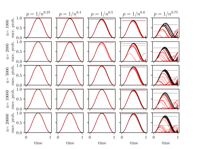
Figure 1: A comparison between the success probabilities for transition rate obtained from the proof in section I from Supplementary materials (solid black lines) [1] and $1/(np)$ (dashed red lines). For each $(n,p)$ pair we took at random 10 Erdős-Rényi graphs. Dotted lines are means of maximum success probability over graphs. The time for each graph is rescaled to $[0,1]$, where $1$ corresponds to $2T$ and $T$ is the optimal time calculated according to the proof of Lemma 1. The code can be found on %****␣comment_paper.tex␣Line␣350␣****https://doi.org/10.5281/zenodo.4055929

4 Minor comments

Reference [14] in the main paper is not correct, since for normalized Laplacian matrix $\mathcal{L}$ attains eigenvalue 2 for bipartite graphs. Hence the proposed Hamiltonian $H_{1}=\mathbb{I}-\mathcal{L}$ has spectral gap equal to zero. The constant normalized algebraic connectivity remains to be a sufficient condition with a Hamiltonian $H_{1}=\mathbb{I}-\frac{2}{3}\mathcal{L}$.

Furthermore, in reference [14] the normalized algebraic connective is defined as the second largest eigenvalue of normalized Laplacian, while it is defined as the smallest positive eigenvalue (which for connected graph is the same as second smallest eigenvalue).

Acknowledgments

AG was partially supported by National Science Center under grant agreement 2019/32/T/ST6/00158 and 2019/33/B/ST6/02011. RK was supported by the Polish National Science Centre under project number 2016/22/E/ST6/00062. The authors would like to thank Aleksandra Krawiec for reviewing the manuscript.

References

[1]
S. Chakraborty, L. Novo, A. Ambainis, and Y. Omar, “Spatial search by quantum
walk is optimal for almost all graphs,” Physical Review Letters,
vol. 116, no. 10, p. 100501, 2016.
[2]
Z. Füredi and J. Komlós, “The eigenvalues of random symmetric
matrices,” Combinatorica, vol. 1, no. 3, pp. 233–241, 1981.
[3]
F. Chung and M. Radcliffe, “On the spectra of general random graphs,” The electronic journal of combinatorics, pp. P215–P215, 2011.
[4]
V. H. Vu, “Spectral norm of random matrices,” in Proceedings of the
thirty-seventh annual ACM symposium on Theory of computing, pp. 423–430,
2005.
[5]
A. Glos, A. Krawiec, R. Kukulski, and Z. Puchała, “Vertices cannot be
hidden from quantum spatial search for almost all random graphs,” Quantum Information Processing, vol. 17, no. 4, p. 81, 2018.