Generating End-to-End Adversarial Examples for Malware Classifiers Using Explainability

Abstract

In recent years, the topic of explainable machine learning (ML) has been extensively researched. Up until now, this research focused on regular ML users use-cases such as debugging a ML model. This paper takes a different posture and show that adversaries can leverage explainable ML to bypass multi-feature types malware classifiers. Previous adversarial attacks against such classifiers only add new features and not modify existing ones to avoid harming the modified malware executable’s functionality. Current attacks use a single algorithm that both selects which features to modify and modifies them blindly, treating all features the same. In this paper, we present a different approach. We split the adversarial example generation task into two parts: First we find the importance of all features for a specific sample using explainability algorithms, and then we conduct a feature-specific modification, feature-by-feature. In order to apply our attack in black-box scenarios, we introduce the concept of transferability of explainability, that is, applying explainability algorithms to different classifiers using different features subsets and trained on different datasets still result in a similar subset of important features. We conclude that explainability algorithms can be leveraged by adversaries and thus the advocates of training more interpretable classifiers should consider the trade-off of higher vulnerability of those classifiers to adversarial attacks.

I Introduction

In recent years, the topic of explainable and interpretable machine learning (ML) has been extensively researched. Explainable machine learning can be used by the ML model users and developers, e.g., to debug prediction errors of an existing ML model on specific samples or to provide human explanations of models’ decisions by highlighting the features that had the highest impact on a specific sample decision.

In this paper, we demonstrate the ability of an adversary to use the explainability of multi-feature types malware classifiers algorithms to produce the most important features for a known, white-box model. Then, due to the concept of transferable explanations, the same important features are relevant to the target black-box classifier. Therefore, by modifying existing malware’s important features by the white-box model’s explanation to fool it, not only the white-box model would be fooled, but also the target black-box model.

The principle of transferability of adversarial examples, that is, adversarial examples crafted against one model are also likely to be effective against other models, is already known [1, 2, 3] and was also evaluated in the cyber security domain [4]. However, most research related to adversarial examples is focused on adversarial examples containing a single feature type: changing pixel’s color in an input image, modifying words in an input sentence, etc. In those cases, modifying each feature has the same level of difficulty, because they all have the same feature type.

In contrast, in the cyber security domain there is a unique challenge which is not addressed by previous research: Malware classifiers (which gets an executable file as input and predict the labels of benign or malicious for each file) often use more than a single feature type (see Section I-A2). Thus, adversaries who want to subvert those systems should consider modifying more than a single feature type. Some feature types are easier to modify without harming the executable functionality than others (see Section I-A2). In addition, even the same feature type might be modified differently depending on the sample format. For instance, modifying a printable string inside a PE file might be more challenging than modifying a word within the content of an email, although the feature type is the same. This means that we should not only take into account the impact of a feature on the prediction, but also the difficulty of modifying this feature type [5]. In addition, some features are dependent on other features, meaning that modifying one feature requires modifying other features for the executable to continue functioning. For instance, adding strings to the file (as done in [4]) will necessarily impact the features dependent on printable characters, e.g., entropy.

The end result is that when adversaries want to modify a PE file without harming its functionality, the feature modification must be done manually. In this way, only features that are easy to modify, not dependent on other features who are challenging to modify (which is feature specific) would be modified. Thus, we would want to modify the smallest numbers of features, because each feature’s modification requires a manual effort. Moreover, each modified feature can create a feature distribution anomaly that could be detected by anomaly detection algorithms (e.g., [6]). Therefore, the adversary aims to modify as little features as possible, even if he/she could modify all features automatically. In order to achieve this goal, the adversary would like to get the list of most impactful features for a specific sample (the malware which tries to bypass the malware classifier) and manually select the features that are the easiest to modify. This is the approach we take in this paper, as opposed to previous adversarial attacks, that try to do both in the same algorithm and thus try to modify all features in the same manner, resulting in generating malware executables that don’t run.

In order to select the most indicative features for a sample, the adversary can use explainability algorithms. However, the adversary is not familiar with the architecture of the target malware classifier. In order to resolve this issue, he/she can train his/her own malware classifier and use its features instead. Those features are likely to have a high impact even in the target classifier, due to the concept of transferability of explainability.

I-A The Challenges in End-To-End Adversarial Examples of Malware Executables

Most published adversarial attacks, including those that were published at academic cyber security conferences have focused on the computer vision domain, e.g., generating a cat image that would be classified as a dog by the classifier. However, the cyber security domain – and particularly the malware detection task - seems a much more relevant domain for adversarial attacks, because while in the computer vision domain, there is no concrete adversary who wants cats to be classified as dogs, in the cyber security domain, there are actual adversaries with clear targeted goals. Examples include ransomware developers who depend on the ability of their ransomware to evade anti-malware products that would prevent both its execution and the developers from collecting the ransom money, and other types of malware that need to steal user information (e.g., keyloggers), spread across the network (worms) or perform any other malicious functionality while remaining undetected.

Given the obvious relevance of the cyber security domain to adversarial attacks, why do most adversarial learning researchers focus on computer vision? Besides the fact that image recognition is a popular machine learning research topic, another major reason is that performing an end-to-end adversarial attack in the cyber security domain is more difficult than performing such an attack in the computer vision domain. The differences between adversarial attacks performed in those two domains and the challenges that arise in the cyber security domain are discussed in the subsections that follow.

I-A1 Executable (Malicious) Functionality

Any adversarial executable must preserve its malicious functionality after the sample’s modification. This might be the main difference between the image classification and malware detection domains, and pose the greatest challenge. In the image recognition domain, the adversary can change every pixel’s color (to a different valid color) without creating an “invalid picture” as part of the attack. However, in the cyber security domain, modifying an API call or arbitrary executable’s content byte value might cause the modified executable to perform a different functionality (e.g., modifying a WriteFile() call to ReadFile() ) or even crash (if you change an arbitrary byte in an opcode to an invalid opcode that would cause an exception).

In order to address this challenge, adversaries in the cyber security domain must implement their own methods (which are usually feature-specific) to modify features in a way that will not break the functionality of the executable. For instance, the adversarial attack used in Rosenberg et al. [4] modifies API call traces in a functionality preserving manner.

I-A2 There are Many Feature Types

In the cyber security domain, classifiers usually use more than a single feature type as input (e.g., malware detection using both PE header metadata and byte entropy in Saxe et al. [7]). Some feature types are easier to modify without harming the executable functionality than others. For instance, in the adversarial attack used in Rosenberg et al. [4], appending printable strings to the end of file is much easier than adding API calls using a dedicated framework built for this purpose. In contrast, in an image adversarial attack, modifying each pixel has the same level of difficulty.

I-A3 Executables are More Complex than Images

An image used as input to an image classifier (usually a convolutional neural network, CNN) is represented as a fixed size matrix of pixel colors. If the actual image has different dimensions than the input matrix, the picture will usually be resized, clipped, or padded to fit the dimension limits.

An executable, on the other hand, has a variable length: executables can range in size from several KB to several GB. It’s also unreasonable to expect a clipped executable to keep its original classification. Let’s assume we have a 100MB benign executable into which we inject a shellcode at a function near the end-of-file. If the shellcode is clipped in order to fit the malware classifier’s dimensions, there is no reason that the file would be classified as malicious, because its benign variant would be clipped to the exact same form.

In addition, the code execution path of an executable may depend on the input, and thus, the adversarial perturbation should support any possible input that the malware may encounter when executed in the target machine.

While this is a challenge for malware classifier implementation, it also affects adversarial attacks against malware classifiers. Attacks in which you have a fixed input dimension, (e.g., a 28*28 matrix for MNIST images), are much easier to implement than attacks in which you need to consider the variable file size.

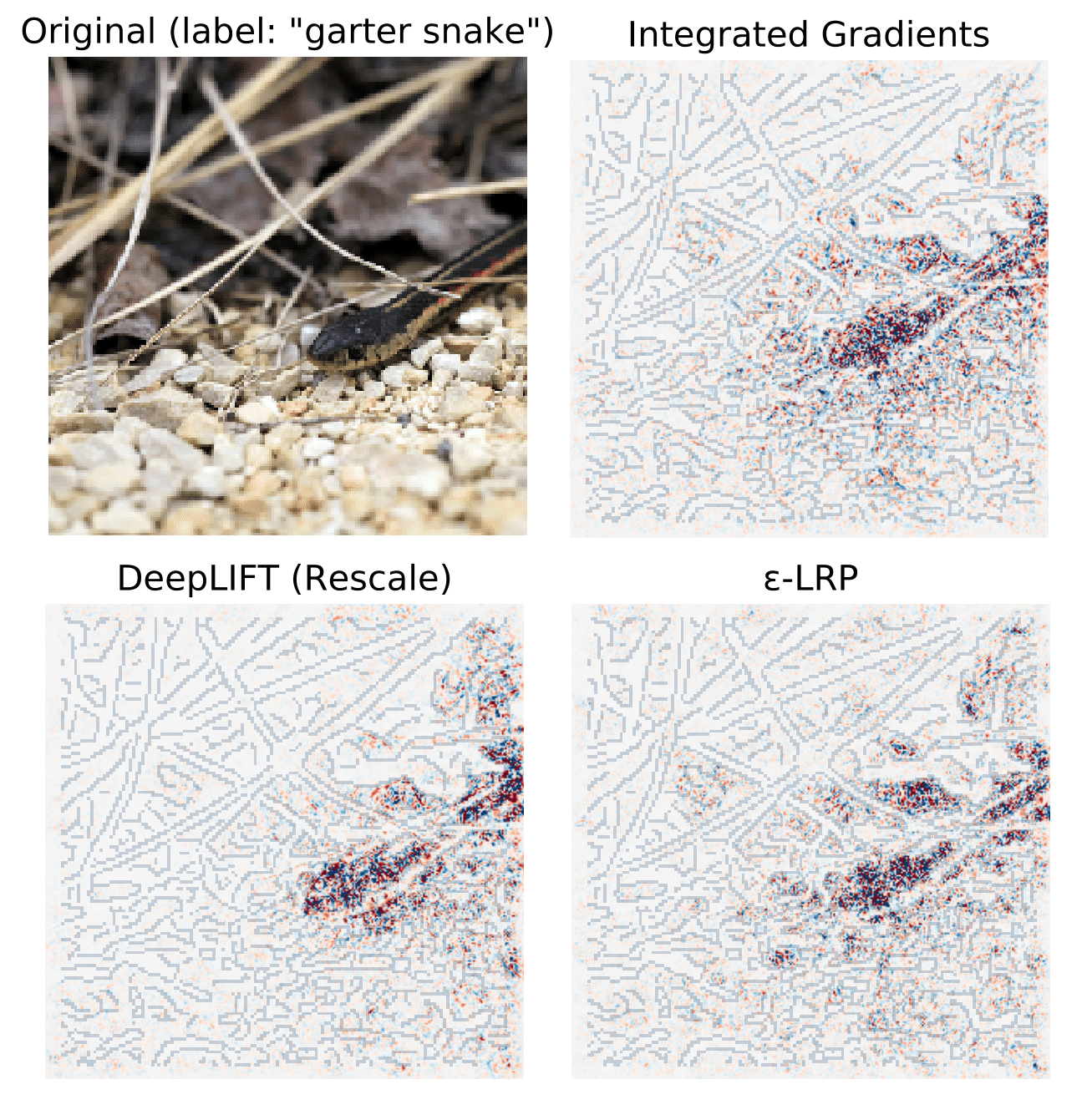
Figure 1: Explainability Algorithms in the Image Recognition Domain (Taken from [8])

The main contributions of this paper are as follows:

1. This is the first paper to demonstrate end-to-end adversarial examples (that is, runnable malware) against malware classifiers that rely on multiple types of interconnected and dependent features. This is also the first such attack which not only adds features, but also modify them while maintaining the malware functionality.

2. This is the first paper to discuss the usage of explainability by adversaries, in order to both choose specific features to perturb and maintain the minimal perturbation (that is, number of perturbed features).

3. This is the first paper analyzing the concept of transferability of explainability, using explainability of a white-box substitute model to explain a black-box model, using a subset of the same indicative features.

II Related Work

II-A Explainable Machine Learning

In this paper, we evaluate the usage of explainability algorithms (which ranks the features by impact on the classification of a specific sample, see Definition 1) in order to generate an adversarial example with a small perturbation size. Several such algorithms have been introduced:

Integrated Gradients [9], computes the partial derivatives of the output with respect to each input feature. Integrated Gradients computes the average gradient while the input varies along a linear path from a baseline $\bar{\boldsymbol{x}}$ to $\boldsymbol{x}$. The baseline is defined by the user and often chosen to be zero. The importance (also known as attribution) of $x_{i}$, the $i$-th element in the vector $\boldsymbol{x}$:

$$R(x_{i})=(x_{i}-\bar{x_{i}})\intop_{\alpha=0}^{1}\frac{\partial C(\boldsymbol{\tilde{x}})}{\partial\tilde{x_{i}}}\mid_{\widetilde{\boldsymbol{x}}=\bar{\boldsymbol{x}}+\alpha(\boldsymbol{x}-\boldsymbol{\bar{x}})d\alpha}$$ (1)

, where $C(\boldsymbol{x})$ is the classifier prediction for $\boldsymbol{x}$. Integrated Gradients satisfies an important property termed completeness: the attributions sum up to the target output minus the target output evaluated at the baseline: $\sideset{}{{}_{i=1}^{N}}{\sum}R(x_{i})=C(\boldsymbol{x})-C(\boldsymbol{\bar{x}})$.

Layer-wise Relevance Propagation (LRP) [10] is computed with a backward pass on the network. Let us consider a quantity $r_{i}^{(l)}$ , called "relevance" of unit $i$ of layer $l$. The algorithm starts at the output layer $L$ and assigns the relevance of the target neuron c equal to the output of the neuron itself and the relevance of all other neurons to zero (Equation 2).

$$r_{i}^{(L)}=\begin{cases}C_{i}(\boldsymbol{x})&if\>unit\>i\>is\>the\>unit\>of\>interest\\ 0&otherwise\end{cases}$$ (2)

The algorithm proceeds layer by layer, redistributing the prediction score $C_{i}$ until the input layer is reached. One recursive rule for the redistribution of a layer’s relevance to the following layer is the $\epsilon-rule$ described in Equation 3, where we define $z_{ji^{\prime}}=w_{ji^{\prime}}^{(l+1,l)}x_{i^{\prime}}^{(l)}+b_{j}$ to be the weighted activation of a neuron i’ onto neuron $j$ in the next layer and $b_{j}$ the additive bias of unit $j$. A small quantity is added to the denominator of Equation 3 to avoid numerical instabilities. Once reached the input layer, the final importance is defined as $R(x_{i})=r_{i}^{(1)}$ .

$$r_{i}^{(l)}=\sideset{}{{}_{j}}{\sum}\frac{w_{ji}^{(l+1,l)}x_{i}^{(l)}}{\sideset{}{{}_{i^{\prime}}}{\sum}\left(z_{ji^{\prime}}\right)+\epsilon*sign\left(\sideset{}{{}_{i^{\prime}}}{\sum}\left(z_{ji^{\prime}}\right)\right)}r_{j}^{(l+1)}$$ (3)

LRP together with the propagation rule described in Equation 3 is called $\epsilon-LRP$, analyzed in the remainder of this paper.

DeepLIFT [11] proceeds in a backward fashion, similarly to LRP. Each unit $i$ is assigned an attribution that represents the relative effect of the unit activated at the original network input $\boldsymbol{x}$ compared to the activation at some reference input $\bar{\boldsymbol{x}}$ (Equation 4).

$$r_{i}^{(L)}=\begin{cases}C_{i}(\boldsymbol{x})-C_{i}(\bar{\boldsymbol{x}})&if\>unit\>i\>is\>the\>unit\>of\>interest\\ 0&otherwise\end{cases}$$ (4)

Reference values $\bar{z_{ji^{\prime}}}$ for all hidden units are determined running a forward pass through the network, using the baseline $\bar{\boldsymbol{x}}$ as input, and recording the activation of each unit. As in LRP, the baseline is often chosen to be zero. The relevance propagation is described in Equation 5. The attributions at the input layer are defined as $R(x_{i})=r_{i}^{(1)}$ as for LRP.

$$r_{i}^{(l)}=\sideset{}{{}_{j}}{\sum}\frac{z_{ji}-\bar{z_{ji}}}{\sideset{}{{}_{i^{\prime}}}{\sum}\left(z_{ji^{\prime}}\right)-\left(\sideset{}{{}_{i^{\prime}}}{\sum}\left(\bar{z_{ji^{\prime}}}\right)\right)}r_{j}^{(l+1)}$$ (5)

In Equation 5, $\bar{z}_{ji^{\prime}}=w_{ji^{\prime}}^{(l+1,l)}\bar{x}_{i^{\prime}}^{(l)}+b_{j}$ is the weighted activation of a neuron $i$ onto neuron $j$ when the baseline $\bar{\boldsymbol{x}}$ is fed into the network. As with Integrated Gradients, DeepLIFT was designed to satisfy Completeness. The rule described in Equation 5 ("Rescale rule") is used in the original formulation of the method and it is the one we will analyze in the remainder of the paper.

[8] formalized the above-mentioned methods in similar terms and found some interesting similarities between them. For instance, all methods are equivalent when the model behaves linearly, e.g., when the network is very shallow.

SHAP (SHapley Additive exPlanation) [12] values also explain the output of a classifier $C$ as a sum of the effects $R(x_{i})$ of each feature being introduced into a conditional expectation. However, unlike the above-mentioned methods, SHAP is a black-box method, which doesn’t require any knowledge about the architecture of the explained network. Therefore, it cannot compute partial derivatives of the gradients with respect to specific features. In order to evaluate the effect missing features have on a model $C$ , it is necessary to define a mapping between the missing features and the original function input space. Therefore, In order to compute SHAP values, we define $C_{x}(S)=E\left(C(x)|x_{S}\right)$ where $S$ is the set of analyzed features, and $E\left(C(x)|x_{S}\right)$ is the expected value of the function conditioned on a subset S of the input features. SHAP values combine these conditional expectations with the classic Shapley values from game theory together to attribute $R(x_{i})$ values to each feature:

$$R(x_{i})=\sideset{}{{}_{S\subseteq F-\{i\}}}{\sum}\frac{|S|!\left(|F-S|-1\right)!}{|F|!}\left[f_{x}\left(S\cup\{i\}\right)-f_{x}\left(S\right)\right]$$ (6)

, where $F$ is the set of all input features. Note that for non-linear functions the order in which features are introduced matters. SHAP values result from averaging over all possible orderings. Proofs from game theory show this is the only possible consistent approach where $\sideset{}{{}_{i=0}^{|F|}}{\sum}R(x_{i})=C(\boldsymbol{x})$. SHAP outperforms other state-of-the-art black-box explainability algorithms, e.g., LIME [13].

Very few papers have been published about explainability in the cyber domain. Gue et al. [13] extends the LIME algorithm to a variant called LEMNA, so it can be used for recurrent neural networks (RNNs), commonly used in the cyber security domain (but not in this paper and therefore it is not being evaluated here). This is done using Gaussian mixture to better handle the non-linearities of RNNs and fused lasso to merge features with similar importance together.

Warnecke et al. [14] have evaluated the explainability of several of the algorithms mentioned above for different datasets in the cyber security domain and concluded that white-box explainability algorithms, such as integrated gradients (Equation 1) and LRP (Equation 3) select features which are both have a higher impact on the classification and provide better human interpretable explanations, comparing to black-box explainability algorithms such as SHAP (Equation 6) and LEMNA [13].

II-B Adversarial Examples

[1] and [15] formalize the search for adversarial examples as a similar minimization problem:

$$\arg_{\boldsymbol{r}}\min C(\boldsymbol{x}+\boldsymbol{r})\neq C(\boldsymbol{x})\>s.t.\>\boldsymbol{x}+\boldsymbol{r}\in\boldsymbol{D}$$ (7)

The input $\boldsymbol{x}$, correctly classified by the classifier $C$, is perturbed with $\boldsymbol{r}$ such that the resulting adversarial example $\boldsymbol{x}+\boldsymbol{r}$ remains in the input domain $\boldsymbol{D}$, but is assigned a different label than $\boldsymbol{x}$. To solve Equation 7, we need to transform the constraint $C(\boldsymbol{x}+\boldsymbol{r})\neq C(\boldsymbol{x})$ into an optimizable formulation. Then we can easily use the Lagrange multiplier to solve it. To do this, we define a loss function $Loss()$ to quantify this constraint. This loss function can be the same as the training loss, or it can be chosen differently, e.g., hinge loss or cross entropy loss.

There are three types of adversarial examples generation methods:

Gradient based attacks - Those adversarial perturbation are generated in the direction of the gradient, that is, in the direction with the maximum effect on the classifier’s output, e.g., FGSM [2] or JSMA [16]) Those attacks are effective but require adversarial knowledge about the targeted classifier’s gradients. Those attacks can be conducted on the targeted model, if white-box knowledge is available, or via the usage of a surrogate model, using the transferability property (Appendix B) for a black-box attack.

Score based attacks - Those attacks are based on white-box knowledge of the confidence score of the target classifier. The target classifier’s gradient can be numerically derived from confidence scores of adjacent input points [17] and then continue like gradient-based attack, following the direction of maximum impact. A different approach is using a genetic algorithm, where the fitness of the genetic variants is defined in terms of the target classifier’s confidence score, to generate adversarial examples [18].

Decision based attacks - These attacks use only the label predicted by the target classifier. [19] starts from a randomly generated image classified as desired and then adds perturbations that decrease the distance to the source class image, while maintaining the target classification. The more noise you add, the larger the chance of successfully modifying the classifier’s decision. However, the challenge is usually to use as little noise as possible, since more noise might damage the original functionality of the input. For instance, adding “benign” API calls to a malware might cause a malware classifier to classify it as benignware, but might also add performance overhead to the modified malware, due to the added API calls. [20] uses Natural Evolutionary Strategies (NES) optimization to enable query-efficient gradient estimation, which leads to generation of misclassified images like gradient based attacks.

II-B1 The Transferability Property

Many black-box attacks (e.g., [4]) rely on the concept of adversarial example transferability, presented in [1]: Adversarial examples crafted against one model are also likely to be effective against other models. This transferability property holds even when models are trained on different datasets. This means that the adversary can train a substitute model, which has similar decision boundaries as the original model and perform a white-box attack on it. Adversarial examples that successfully fool the surrogate model would most likely fool the original model, as well ([21]).

The transferability between DNNs and other models such as decision tree and SVM models was examined in [3]. The reasons for the transferability are unknown yet, but a recent study [22] suggests that adversarial vulnerability is not “necessarily tied to the standard training framework, but is rather a property of the dataset (due to representation learning of non robust features)”, which also clarifies why transferability happens regardless of the classifier architecture.

II-B2 End-To-End Adversarial Examples against Malware Classifiers

Attacks vary based on the amount of knowledge the adversary has about the classifier being subverted: Black-Box attacks requires no knowledge about the model beyond the ability to query it as a black-box (a.k.a. the oracle model), i.e., inserting an input and getting the output classification, while white-Box attacks assume the adversary has knowledge about the model architecture and even the hyperparameters used to train the model. In this paper, we focus in black-box attacks, which are a more realistic scenario in the cyber security domain, in which security vendors don’t reveal their architecture to avoid being copied or bypassed.

Grosse et al. [23] presented a white-box attack against an Android static analysis fully connected DNN malware classifier. The static features used were from the AndroidManifest.xml file, including permissions, suspicious API calls, activities, etc. The attack is a discrete FGSM [2] variant, which is performed iteratively in two steps, until a benign classification is achieved: (1) Compute the gradient of the white-box model with respect to the binary feature vector $\boldsymbol{x}$. (2) Find the element in $\boldsymbol{x}$ whose modification from zero to one (i.e., only feature addition and not removal) would cause the maximum change in the benign score, and add this manifest feature to the adversarial example. Unlike our attack, Grosse et al. only adds features and the APK format used is much simpler than the PE format used in our attack, with no interdependent features.

Xu et al. [18] generated adversarial examples that bypass PDF malware classifiers, by modifying static PDF features. This was done using an inference integrity genetic algorithm (GA), where the fitness of the genetic variants is defined in terms of the target classifier’s confidence score. The GA is computationally expensive and was evaluated against SVM, random forest, and CNN using static PDF structural features. This attack requires knowledge of both the classifier’s features and the target classifier’s confidence score. Unlike our attack, Xu et al. only adds features and the PDF format used is much simpler than the PE format used in our attack, with no interdependent features.

Suciu et al. [24] implemented an attack against MalConv, a 1D CNN, using the file’s raw byte content as features (Raff et al. [25]). The additional bytes are selected by the FGSM method and are inserted between the file’s sections. in a black-box manner by appending bytes from the beginning of benign files. Unlike our attack, Suciu et al. use only a single feature type (raw bytes) and only add features (and not modify features), which is a less realistic scenario than ours.

Rosenberg et al. [4, 26] presented a black-box inference integrity attack that adds API calls to an API call trace used as input to an RNN malware classifier in order to bypass a classifier trained on the API call trace of the malware. A GRU substitute model was created and attacked, and the transferability property was used to attack the original classifier. The authors extended their attack to hybrid classifiers combining static and dynamic features, attacking each feature type in turn. The target models were LSTM variants, GRUs, conventional RNNs, bidirectional and deep variants, and non-RNN classifiers (including both feedforward networks, like fully connected DNNs and 1D CNNs, and traditional machine learning classifiers, such as SVM, random forest, logistic regression, and gradient boosted decision tree). The authors presented an end-to-end framework that creates a new malware executable without access to the malware source code. Unlike our attack, Rosenberg et al. only adds features, not modify them and only uses two feature types, which are independent, making this case less challenging and realistic than ours.

In Anderson et al. [27], the features used by the gradient boosted decision tree classifier included PE header metadata, section metadata, and import/export table metadata. A black-box attack which trains a reinforcement learning agent was presented. The agent is equipped with a set of operations (such as packing) that it may perform on the PE file. The reward function was the evasion rate. Through a series of games played against the target classifier, the agent learns which sequences of operations are likely to result in detection evasion for any given malware sample. The differences from our attack are: (1) Our attack also achieve higher attack effectiveness then Anderson et al. with less adversary’s knowledge (different classifier’s type and architecture, training set and feature subset), due to our usage of transferability of explainability. (2) The attack in Anderson et al. uses whole-PE transformations like packing, which increases the chances of the generated malware to be detected by anomaly detection methods (e.g., [6]). (3) Our attack effectiveness is 37%, as opposed to less than 25% for Anderson et al. on the same dataset and using the same attacked classifier. Note that both attacks have a lower effectiveness than image-based attacks due to the challenges mentioned in Section I-A.

This paper is the first to present end-to-end PE structural features adversarial examples, which, unlike previous attacks, include feature modification (and not just addition) without harming the malware functionality and interdependent features.

II-B3 Using Explainable ML in Adversarial Scenarios

Several papers have tried to leverage the usage of explainability to detect adversarial examples, although none of them are in the cyber security domain.

Tau et al. [28] generated a mapping to the neurons critical for specific attributes and amplified the activation of those neurons to make the classifier more robust to adversarial attacks. Carlini [29] demonstrated that this robust classifier is still vulnerable to the Carlini and Wagner attack.

Fidel et al. [30] used the SHAP values computed for the internal layers of a DNN classifier to discriminate between normal and adversarial inputs. Amosy et al. [31] used a similar approach.

To the best of our knowledge, our paper is the first to leverage explainability algorithms from the adversary side, to generate and facilitate adversarial attacks (as opposed to detecting them).

III Methodology

III-A Threat Model

The adversary’s goal is to modify a malware executable for it to bypass a multi-feature types malware classifier without harming the executable’s functionality (Section I-A1), that is, generating an end-to-end malware adversarial example. In this paper we limit ourselves to static features, that is, features that can be extracted from the file without running it. Static features are the malware file’s content and properties (e.g., the file’s size) either as raw bytes or pre-processed to parse them in the way used by the operating system loads them, termed PE structural features. Raw-byte features require a very long training process and current state-of-the-art GPU hardware usually limits the file size which can be classified using such classifier (e.g. [25]), making this a non realistic use case. Using dynamic features (e.g., executed API calls in Rosenberg et al. [4]) is also less common use case, since it requires a sandbox environment in order to avoid running a malware on the computer we want to protect, which might harm it. We therefore decided to focus on PE structural features, which are used by real-world classifiers. We assume the adversary has no knowledge or access to the attacked malware classifier, e.g., the classifier type, architecture or training set (a black-box attack, as defined in Section II-B2). Our attack would be a decision-based attack (by the definition in Section II-B), as this is the most realistic scenario. We do assume the adversary can figure out some of the features used by the attacked malware classifier, but not all of them. This is a common case in cyber security, especially with static features, where many classifiers are using similar PE structural features, (e.g., [7, 27, 32]) but the exact subset of features is unknown.

III-B Generating an End-to-End Adversarial Example

In order to evade detection by the malware classifier, the adversary is using the method specified in Algorithm 1.

Algorithm 1 End-to-End PE Structural Features-Based Adversarial Example Generation

1. Train a substitute neural network model on a training set and features believed to accurately represent the attacked malware classifier.

2. Select a malware binary he/she wants to bypass the attacked malware classifier.

3. Use explainable machine learning algorithm (see Definition 1) to get a list of features importance for the classification of the malware on the substitute model (see Section IV-B).

4. From those features, choose those easier to modify (see Section III-D3).

5. Modify each “easily modifiable” feature using the list of predefined feature values (see Section III-D3), selecting the value that result in the lowest confidence score. Repeat until a benign classification is achieved by the target black-box malware classifier.

In this method, we use the following definition:

Definition 1.

An explainable machine learning algorithm $A(m,\boldsymbol{v})$ takes as arguments a machine learning model $m$ and a sample’s vector $\boldsymbol{v}$ and returns a vector of $length(\boldsymbol{v})$ values which represent the weights of impact of the features in $\boldsymbol{v}$, such that a higher weight indicates a more impactful feature for classifying the vector $\boldsymbol{v}$ by the model $m$.

This method is relying on two assumptions, evaluated in the following subsections:

(1) The most important features in the attacked malware classifier would be similar to those of the substitute model, and they would also be found by an explainability algorithm. Thus, modifying these features in the method mentioned above would affect the attacked malware classifier as well. Detailed in Section III-C, and (2) The adversary can modify the malware binary without harming its functionality. Detailed in Section III-D.

III-C Transferability of Explainability

The concept of transferability of explainability is defined as follows:

Definition 2.

Given two different models, $m_{1}$ and $m_{2}$ with different classifier type and architecture trained on a similar dataset and input features list, the output of an explainable machine learning algorithm (see Definition 1) would be similar for $m_{1}$ and $m_{2}$.

Note that this definition is different from adversarial examples transferability: Adversarial examples transferability (see Section II-B1) is the concept of an adversarial example generated to fool one classifier is also effective against another classifier. Transferability of explainability means that the feature group indicated to have a high impact on a specific sample classification on one model would be similar to the list of the same explainability algorithm on another model. We argue that this holds true regardless of the classifier type, architecture, training set or even explainable algorithm. The only requirement is that the features used by both classifiers need to be similar enough (otherwise impactful features in one model are meaningless in the other model) - but not identical. A visual example of the transferability of explainability can be seen in Figure 1. We see that three different explainable algorithms (Integrated Gradients [9], DeepLIFT [11] and Layer-wise Relevance Propagation (LRP) [10]) highlight similar features as the most important to classify a gartner snake image (mainly, pixels in the snake’s head area).

This concept is especially important for multi-feature types malware classifiers: On the one hand, the adversary is unaware of the attacked classifier architecture, so using transferability is essential. On the other hand, modifying too many features might cause the adversarial example to be caught by anomaly detectors (e.g., [6]). Therefore, a small perturbation (that is, modifying a small amount of features) is desired.

Using transferability of explainability to generate adversarial examples is also usable in scenarios where using transferability of adversarial examples (as done in the adversarial attacks mentioned in Section II-B for a black-box scenario) is not:

(1) When there are dependent features, which modification requires the modification of other features for the file to continue being runnable, as in the case of PE structural features, discussed in this paper (see Section III-D2). In this case, it’s very hard to take into account which features need to be modified to keep a small perturbation automatically.

(2) When some features are harder to modify than others, which is very hard to take into account in any mathematical form [5], which can be used automatically.

In contrast, a manual modification of the features by their order of impact is a preferable approach to keep the perturbation small. Such cases might be the reason why there are no adversarial attacks published on end-to-end PE structural features yet (see Section II-B2).

III-D End-to-End Feature Modification for PE Structural Features

In this paper we are focusing on malware running on Windows OS, since most malware target the Windows OS. Thus, we focus on the static features of the executable format on Windows, named portable executable (PE).

III-D1 PE Structural Features Overview

In this section we discuss the features that exist in the dataset used in this paper, Ember. However, as mentioned in Section III-A, many classifiers are using similar PE structural features, so this description is valid to all of them. A more detailed list of the Ember model features appear in [32]. Here we will only describe some major key points regarding the feature types used in the model. Some features are naive values extracted from the PE header with no modification at all and some features are engineered, for example, string features which count occurrences of Windows path strings. On a high-level, the PE file itself is composed of the PE header, sections and overlay. The PE header in turn is composed of various fields and additional headers, e.g., DOS header and Optional-Header. The sections are either code sections (machine instructions), data sections (holding variables) and resource sections (holding embedded fonts, images, etc). The overlay is defined as any addition to the PE file that is not defined in the various fields in the headers and therefore not loaded into the process memory. The PE structure has a lot of flexibility. For example, there are numerous entries to describe a section but only few are necessary. Moreover, some values differ when loaded into memory and when viewed statically as they appear in the file. For example, various offsets and relocation are resolved by the Windows process loader and the values are modified during process mapping preparation before executing it.

Feature types description

The different feature types in Ember model are:

(1) Byte histogram - A total of 256 features that describe the byte value histogram in the entire file.

(2) Byte entropy histogram - A total of 256 features that roughly approximates the joint distribution of byte value and local entropy (see [7]).

(3) String related features - A total of 104 string related features, s.a., total count, average string length, Windows path count, etc. 96 features of this group are printable character distribution. We will mostly focus on this subset of the string features.

(4) General information features - A total of 10 features describing properties of the PE file, e.g., import and export functions count, has relocation table, has resource table, etc.

(5) COFF header features - A total of 62 features describing values from the COFF header. Out of these, 50 features use the hash trick with 10 buckets over 5 fields in the COFF header.

(6) Section features - A total of 255 features describing values from the section headers. Out of these, 5 are counters and the other 250 features are hash trick with 50 buckets over 5 fields.

(7) Imports features - A total of 1280 features. All use the hash trick, 256 hash buckets for import library names and 1024 for imported function names.

(8) Exports features - A total of 128 features. All use the hash trick for exported function names.

(9) Data directories features - A total of 30 features, describing values of size and virtual size for 15 data directories entries present in the PE.

III-D2 Feature Modification Challenges

Our goal is to change the model prediction for a given PE file, while not harming the functionality of the PE (Section I-A1). It is easy to see that some feature types are interdependent, for example, modifying some of the string features will affect the byte histogram and byte entropy histogram. Other features may prove to be difficult to near impossible to modify. For example, the hash buckets values can be affected by inserting the relevant value and making sure that the generated hash falls in the required bucket, however it is not always possible to use the resulting value(s) in every field. With strings it may be simple but changing certain values in the header might render the PE file as non executable. It is important to notice that we can only affect feature values in a limited way. Some values cannot be altered, for example if an import function is being used, we will not able to alter the value of the hash bucket to other than a non-zero value.

III-D3 Easily Modifiable PE Structural Features

Analyzing the feature types mentioned above, we notice that there are types of features which can be modified easily without affecting the execution of the PE file as a process when loaded into memory by the OS (and thus the modified PE file’s functionality).

One such example is the printable character distribution (Section III-D1). Considering the character distribution features, we needed to not only keep the values that resulted in the greater shift in prediction score but also recalculate the entire distribution of characters in the file and generate a buffer that when appended to the original file will tilt the distribution accordingly. That buffer can be appended to the end of the file (overlay) but we also chose to insert it as a new section to the PE file, therefore making it a little less trivial to explain the prediction score difference change by an examining eye. The buffers themselves were bound by size but in most test cases we only need several hundred kilo-bytes of data to successfully shift the prediction.

Other features we can modify come mostly from the PE header and its composing headers and values. Listed below is a short description of such features: (1) PE COFF Header timedate stamp - 4 bytes that hold the linkage time of the executable. It has no affect whatsoever on the execution of the PE file. (2) PE CLR Runtime Size - A field that describes the .Net runtime size, used only by the .NET VM when the pe is linked with mscoree.dll (3) PE CLR Runtime Virtual Address - A field that describes the .Net header virtual address, used only by the .NET VM when the pe is linked with mscoree.dll . The features we perturbed can be seen in our git repository.

For each feature, our attack (Algorithm 1, step 5) iterates over a list of predetermined features and alters each of them according to a predefined set of values that matches the feature type possible values. The predefined list of values per feature serves two purposes:

(1) It limits the amount of iterations it takes to complete the brute-force for a specific file, and (2) It verifies that the value ranges fits the feature. For instance, the header feature MajorOperatingSystemVersion is the minimum version of the operating system required to use this executable. Putting a large value (e.g., Windows 10) might prevent the Windows loader from running the modified file on relevant machines (e.g., Windows 7 hosts).

IV Experimental Evaluation

IV-A Dataset and Classifiers

As mentioned in Section III-D1, we used the Ember dataset. It is thoroughly described in [32], and is the state-of-the-art dataset of 1M malware and benign-ware, equally distributed. We split the dataset into a training-set of 300K malware and 300K benignware and a test set of 200K malware and 200K benignware.

As the target classifier, we used the gradient boosted decision tree (GBDT) classifier used in [32], which outperformed state-of-the-art raw features model [25]. This classifier input is a vector of 2381 Ember’s PE structural features and its output is a binary classification: malicious or benign file. It is trained using LightGBM with 100 trees and 31 leaves per tree.

As a substitute model, trained by the adversary, we used an architecture similar to the one used in Saxe et al. [7], which also uses PE structural features. It contains two hidden dense layers with 128 neurons, ReLU activation functions and dropout rate of 0.2, followed by a final dense layer with a sigmoid activation layer. The input and output are identical to the attacked malware classifier. The substitute model was trained with keras, using a tensorflow backend.

IV-B Transferability of Explainability for PE Structural Features Based Multi-Feature Type Malware Classifiers

We want to evaluate the concept of transferability of explainability (Section III-C) in our setting. Mainly, we want to show that the most impactful features in the substitute model are similar to those in the attacked classifier, allowing the adversary to have only black-box access to the attacked malware classifier. We therefore want a measure of the correspondence between two rankings. We evaluated three metrics: We used Kendall’s tau [33] to compare between the feature rankings of different classifiers. Kendall’s tau between two rankins, $\boldsymbol{r_{1}}$ and $\boldsymbol{r_{2}}$, with the same number of elements, is defined as:

$$\tau(\boldsymbol{r_{1}},\boldsymbol{r_{2}})=\frac{P-Q}{\sqrt{(P+Q+T)*(P+Q+U)}}$$ (8)

, where $P$ is the number of agreeable (concordant) pairs, $Q$ the number of non-agreeable (discordant) pairs, $T$ the number of ties (two elements are the same) in $\boldsymbol{r_{1}}$, and $U$ the number of ties in $\boldsymbol{r_{2}}$. If a tie occurs for the same pair in both $\boldsymbol{r_{1}}$ and $\boldsymbol{r_{2}}$, it is not added to either $T$ or $U$. Values close to 1 indicate strong agreement (and transferability), values close to -1 indicate strong disagreement (and lack of transferability) between the ranking orders of the two classifiers. Kendall’s tau has advantages over other rank metrics such-as Spearman’s rho: The distribution of Kendall’s tau has better statistical properties, and the interpretation of Kendall’s tau in terms of the probabilities of observing the agreeable and non-agreeable pairs is very direct.

We also evaluated a variant of the weighted Kendall’s tau [34] metric. The weighted Kendall’s tau is a weighted version of Kendall’s tau in which exchanges of high weight are more influential than exchanges of low weight. We used the metric: $\tau w_{pos}(\boldsymbol{r_{1}},\boldsymbol{r_{2}})$ use additive hyperbolic weighing, that is, rank $r$ is mapped to weight $1/(r+1)$, which has been shown to provide the best balance between important and unimportant elements [34]. Note that $\tau w_{pos}(\boldsymbol{r_{1}},\boldsymbol{r_{2}})$ gives more weight to important features, while $\tau(\boldsymbol{r_{1}},\boldsymbol{r_{2}})$ weighs all features the same.

We evaluated four different state-of-the-art explainability algorithms. We focused on white-box explainability algorithms on the substitute model because [14] showed that this yields better results for cyber security classifiers. Therefore, we evaluated: Integrated Gradients [9], DeepLIFT [11] and $\epsilon-LRP$ [10] (see Section II-A). We compared these methods to the black-box explainability algorithm SHAP [12]. Each of these algorithms’ feature ranks were used to compare between our substitute model and the attacked malware classifier (detailed in Section IV-A), on various levels of knowledge of the adversary:

(1) The substitute model has the same training set and features as the attacked classifier but a different architecture.

(2) The substitute model has the same features as the attacked classifier but a different training set and architecture.

(3) The substitute model has different feature subset, training set and architecture.

In our evaluation, the different architectures of the substitute and attacked malware classifiers are specified in Section IV-A. Different training sets were obtained by randomly dividing the Ember training set (specified in Section IV-A) into two equal-sized training sets of 300K samples (150K malicious, 150K benign) each, used by the attacked malware classifier and the other by the substitute model. This means there wasn’t even a single shared sample, but the samples were from the same distribution (e.g., same prominent malware families were represented in both training sets), as expected in real-world cases. The accuracy of the attacked classifier on the test set is 97.57% (95.55% for the substitute model). When training the same classifier on half the training set, the accuracy reduces to 97.23% (90.81% for the substitute model), so the drop in accuracy is not big. Different features were obtained by randomly picking two subsets of 1190 of Ember’s 2381 features (50% of the features). This resulted in 32% of the 2381 features being used by both attacked and substitute classifiers, resulting in a reduced attack surface, because only those features can be modified and affect the attacked model. This emulates the real world scenario where many malware classifiers use similar feature subsets (see Section III-A). When training the attacked classifier on half the training set using 50% of the features (the same subset used in our attacks), the accuracy reduces to 96.77% (88.94% for the substitute model), so the drop in accuracy is not big here either. The false positive rate of all three models was about 1%. The substitute model achieved similar false positive rate on the test set in all evaluated scenarios mentioned above. The results are shown in Table I. When a random subset was made (whether in the training set or the features), the same random permutation was used in all use cases in the table. We used the explainability algorithms implementation in DeepExplain. We used the Kendall’s tau and weighted Kendall’s tau implementation of scipy. The baseline $\bar{x}$ for the integrated gradients and DeepLIFT methods was chosen as a vector of zeros.

TABLE I: Transferability of Explainability by ($\tau w_{pos}(\boldsymbol{r_{1}},\boldsymbol{r_{2}})$ | $\tau(\boldsymbol{r_{1}},\boldsymbol{r_{2}})$) Metrics

Explainability Algorithm\Adversary’s Knowledge	Same training set and features	Different training set, same features	Different training set and feature subset
Integrated Gradients [9]	0.998 | 0.991	0.969 | 0.832	0.928 | 0.660
DeepLIFT [11]	0.998 | 0.992	0.962 | 0.797	0.923 | 0.641
$\epsilon-LRP$[10]	0.998 | 0.992	0.963 | 0.801	0.926 | 0.652
SHAP [12]	0.997 | 0.989	0.981 | 0.889	0.934 | 0.682
Random Feature Ranking	0.114 | 0.001	0.123 | 0.013	0.018 | 0.007

We see that all the explainability algorithms operating on the substitute model reach a much better correlation (or ranking similarity) between the feature importance in the substitute and attacked models than random feature ranking. Unlike [14] , we see that SHAP is on par with the other, white-box explainability algorithms, possibly due to the different metric we used, which fit our use case of selecting the features to perturb. This high correlation, very close to 1.0, shows that the transferability of explainability does exist in our setting, and the most important features explaining the substitute model’s classification can just as well explain (and affect) the classification of the attacked model. We see that, as expected, the correlation (or ranking similarity) between the feature rankings decreases, as expected when the attacker has less information about the training set or the features. However, even under those constraints, the correlation is relatively high. We also see that $\tau w_{pos}(\boldsymbol{r_{1}},\boldsymbol{r_{2}})$ provides higher correlation than $\tau(\boldsymbol{r_{1}},\boldsymbol{r_{2}})$ in all cases. This shows that while the ranking might be different, the most important features (which are what important for our attack, described in Algorithm 1) are still ranked similarly.

IV-C PE Structural Features Based Multi-Feature Type Malware Classifier End-to-End Adversarial Examples

In order to measure the performance of an attack, we consider two factors:

The attack effectiveness is the percentage of malicious samples which were correctly classified by the attacked malware classifier, for which the end-to-end adversarial example generated by Algorithm 1 was misclassified as benign by the attacked malware classifier.

The average perturbation size is the average number of features (out of the Ember dataset’s total of 2381) that were perturbed before the attack was successful. The adversary aims to minimize it in-order to evade detection by, e.g., anomaly detection classifiers that recognize anomalous PE structure [6].

We generated end-to-end adversarial examples to all the malicious samples in the Ember test set which were correctly detected by the attacked malware classifier (a total of: 97570 samples). The results of the attack are shown in Table II.

TABLE II: Adversarial Examples Success Rate and Average Number of Modified Features

Explainability Algorithm\Adversary’s Knowledge	Same training set and features	Different training set, same features	Different training set and feature subset
Integrated Gradients [9]	37.71% | 3.46	34.63% | 3.83	34.19% | 3.88
DeepLIFT [11]	37.71% | 3.45	34.38% | 3.86	34.01% | 3.91
$\epsilon-LRP$[10]	37.70% | 3.46	34.42% | 3.86	34.13% | 3.90
SHAP [12]	37.66% | 3.47	35.06% | 3.79	34.42% | 3.87
Random Feature Ranking	36.36% | 4.10	11.54% | 3.63	0.11% | 7.91

We see that the regardless of which explainability algorithm we use, the attack effectiveness is very similar. While reducing the attacker knowledge brings to lower attack accuracy and higher number of modified features, the attack is still effective for more than third of the malware, even with different training sets and when only 32% of the features to perturb are known. Selecting the most important features of a random feature ranking (which is equal to random feature selection), brings interesting results. When the attacker has full knowledge about the attacked classifier, the attack effectiveness is not much worse than using the substitute model for selecting the important features to perturb. However, when the attacker has less knowledge (as usually happens in real-world scenarios), the random selction attack effectiveness is significantly reduced. This shows the power and importance of using the explainability approach in real-world scenarios.

V Conclusions and Future Work

In this paper, we present a method to generate end-to-end multi-feature types adversarial examples for PE malware classifiers, using explainability algorithms to decide which features to modify. Our method is the first to tackle the challenging task of generating end-to-end adversarial examples of PE structural features, allowing not only feature addition but also feature modification.

Our evaluation demonstrates that explainability is a dual edged sword, which can also be leveraged by adversaries. When considering the call to generate more explainable models, which decisions can be interpreted by humans [35] , one should take into account its negative effects, such as making adversarial examples less challenging in certain situations, as presented in this paper.

Our future work will include improving the query-efficiency of our attack (in sense of queries to the attacked malware classifier), in order to make it useful to attack cloud-based classifiers, by using gradient-based approaches (e.g., JSMA [16]) over the substitute model in order to find the optimal feature modification out of the initial predetermined list. We would also research the detection and defense methods against such attacks, for instance, anomaly detection classifiers that recognize anomalous PE structure.

References

- [1] C. Szegedy, W. Zaremba, I. Sutskever, J. Bruna, D. Erhan, I. J. Goodfellow, and R. Fergus, “Intriguing properties of neural networks,” vol. abs/1312.6199, 2014.
- [2] I. J. Goodfellow, J. Shlens, and C. Szegedy, “Explaining and Harnessing Adversarial Examples,” ICLR, Dec. 2015.
- [3] N. Papernot, P. D. McDaniel, and I. J. Goodfellow, “Transferability in machine learning: from phenomena to black-box attacks using adversarial samples,” ArXiv e-prints, vol. abs/1605.07277, 2016.
- [4] I. Rosenberg, A. Shabtai, L. Rokach, and Y. Elovici, “Generic black-box end-to-end attack against state of the art API call based malware classifiers,” in RAID, 2018, pp. 490–510.
- [5] Z. Katzir and Y. Elovici, “Quantifying the resilience of machine learning classifiers used for cyber security,” Expert Systems with Applications, vol. 92, pp. 419 – 429, 2018.
- [6] M. Zakeri, F. F. Daneshgar, and M. Abbaspour, “A static heuristic approach to detecting malware targets,” Security and Communication Networks, vol. 8, no. 17, pp. 3015–3027, 2015.
- [7] J. Saxe and K. Berlin, “Deep neural network based malware detection using two dimensional binary program features,” in MALWARE, oct 2015.
- [8] M. Ancona, E. Ceolini, C. Oztireli, and M. Gross, “Towards better understanding of gradient-based attribution methods for deep neural networks,” in ICLR, 2018.
- [9] M. Sundararajan, A. Taly, and Q. Yan, “Axiomatic attribution for deep networks,” in ICML, 2017, pp. 3319–3328.
- [10] S. Bach, A. Binder, G. Montavon, F. Klauschen, K.-R. Müller, and W. Samek, “On pixel-wise explanations for non-linear classifier decisions by layer-wise relevance propagation,” PLoS ONE, vol. 10, no. 7, p. e0130140, 07 2015.
- [11] A. Shrikumar, P. Greenside, and A. Kundaje, “Learning important features through propagating activation differences,” in ICML, 2017, pp. 3145–3153.
- [12] S. M. Lundberg and S.-I. Lee, “A unified approach to interpreting model predictions,” in NIPS, 2017, pp. 4765–4774.
- [13] W. Guo, D. Mu, J. Xu, P. Su, G. Wang, and X. Xing, “LEMNA: explaining deep learning based security applications,” in ACM CCS, 2018, pp. 364–379.
- [14] A. Warnecke, D. Arp, C. Wressnegger, and K. Rieck, “Don’t paint it black: White-box explanations for deep learning in computer security,” CoRR, vol. abs/1906.02108, 2019.
- [15] B. Biggio, I. Corona, D. Maiorca, B. Nelson, N. Šrndić, P. Laskov, G. Giacinto, and F. Roli, “Evasion attacks against machine learning at test time,” in KDD, 2013, pp. 387–402.
- [16] N. Papernot, P. McDaniel, S. Jha, M. Fredrikson, Z. B. Celik, and A. Swami, “The limitations of deep learning in adversarial settings,” in EuroS&P, mar 2016.
- [17] P.-Y. Chen, H. Zhang, Y. Sharma, J. Yi, and C.-J. Hsieh, “Zoo: Zeroth order optimization based black-box attacks to deep neural networks without training substitute models,” in AISec, 2017.
- [18] W. Xu, Y. Qi, and D. Evans, “Automatically evading classifiers: A case study on PDF malware classifiers,” in NDSS, 2016.
- [19] W. Brendel, J. Rauber, and M. Bethge, “Decision-based adversarial attacks: Reliable attacks against black-box machine learning models,” in ICLR, 2018.
- [20] A. Ilyas, L. Engstrom, A. Athalye, and J. Lin, “Black-box adversarial attacks with limited queries and information,” in ICML, 2018, pp. 2142–2151.
- [21] N. Papernot, P. McDaniel, I. Goodfellow, S. Jha, Z. B. Celik, and A. Swami, “Practical black-box attacks against machine learning,” in Asia CCS, ser. ASIA CCS ’17, 2017, pp. 506–519.
- [22] A. Ilyas, S. Santurkar, D. Tsipras, L. Engstrom, B. Tran, and A. Madry, “Adversarial examples are not bugs, they are features,” arXiv preprint arXiv:1905.02175, 2019.
- [23] K. Grosse, N. Papernot, P. Manoharan, M. Backes, and P. McDaniel, “Adversarial examples for malware detection,” in ESORICS, 2017, pp. 62–79.
- [24] O. Suciu, S. E. Coull, and J. Johns, “Exploring adversarial examples in malware detection,” in ALEC, 2018, pp. 11–16.
- [25] E. Raff, J. Barker, J. Sylvester, R. Brandon, B. Catanzaro, and C. K. Nicholas, “Malware detection by eating a whole EXE,” in AAAI Workshop, 2018, pp. 268–276.
- [26] I. Rosenberg, A. Shabtai, Y. Elovici, and L. Rokach, “Query-efficient black-box attack against sequence-based malware classifiers,” CoRR, vol. abs/1804.08778, 2018.
- [27] H. S. Anderson, A. Kharkar, B. Filar, D. Evans, and P. Roth, “Learning to evade static PE machine learning malware models via reinforcement learning,” CoRR, vol. abs/1801.08917, 2018.
- [28] G. Tao, S. Ma, Y. Liu, and X. Zhang, “Attacks meet interpretability: Attribute-steered detection of adversarial samples,” in NeurIPS, 2018, pp. 7728–7739.
- [29] N. Carlini, “Is ami (attacks meet interpretability) robust to adversarial examples?” CoRR, vol. abs/1902.02322, 2019.
- [30] G. Fidel, R. Bitton, and A. Shabtai, “When explainability meets adversarial learning: Detecting adversarial examples using SHAP signatures,” CoRR, vol. abs/1909.03418, 2019.
- [31] O. Amosy and G. Chechik, “Using explainabilty to detect adversarial attacks,” 2020.
- [32] H. S. Anderson and P. Roth, “EMBER: an open dataset for training static PE malware machine learning models,” CoRR, vol. abs/1804.04637, 2018.
- [33] M. G. Kendall, “The treatment of ties in ranking problems,” Biometrika, vol. 33, no. 3, pp. 239–251, 1945.
- [34] S. Vigna, “A weighted correlation index for rankings with ties,” in Proceedings of the 24th International Conference on World Wide Web, ser. WWW 15, 2015, pp. 1166–1176.
- [35] C. Rudin, “Please stop explaining black box models for high stakes decisions,” CoRR, vol. abs/1811.10154, 2018.