An AI approach to measuring financial risk

Abstract

AI artificial intelligence brings about new quantitative techniques to assess the state of an economy. Here we describe a new measure for systemic risk: the Financial Risk Meter (FRM). This measure is based on the penalization parameter ($\lambda$) of a linear quantile lasso regression. The FRM is calculated by taking the average of the penalization parameters over the 100 largest US publicly traded financial institutions. We demonstrate the suitability of this AI based risk measure by comparing the proposed FRM to other measures for systemic risk, such as VIX, SRISK and Google Trends. We find that mutual Granger causality exists between the FRM and these measures, which indicates the validity of the FRM as a systemic risk measure. The implementation of this project is carried out using parallel computing, the codes are published on www.quantlet.de with keyword  FRM. The R package RiskAnalytics is another tool with the purpose of integrating and facilitating the research, calculation and analysis methods around the FRM project. The visualization and the up-to-date FRM can be found on hu.berlin/frm.

Keywords: Systemic Risk, Quantile Regression, Value at Risk, Lasso, Parallel Computing, Financial Risk Meter

JEL: C21, C51, G01, G18, G32, G38.

This is a post-peer-review, pre-copyedit version of an article published in the Singapore Economic Review. The final authenticated version is available online at:
http://dx.doi.org/10.1142/S0217590819500668

1 Introduction

Systemic risk is hazardous for the stability of financial markets, since the failure of one firm may impact the stability of the whole system. There are various definitions of systemic risk. One of the most popular definitions is introduced in Schwarcz (2008). He defined systemic risk as a trigger event, such as an economic shock or institutional failure, causing a chain of bad economic consequences, sometimes referred to as domino effect. This definition indicates that interlinkages and interdependencies in a system or market are very crucial for controlling systemic risk. The financial crisis in 2008 is an example. After the bankruptcy of Lehman Brothers, several more financial cooperations bankrupted as a result of their interlinkages with Lehman Brothers. Consequently, there has been a surge in the interest in measuring and controlling systemic risk since the 2008 crisis, which has led to an increase in the research on this topic.

Several methodologies for measuring systemic risk have been proposed. Adrian and Brunnermeier (2016) proposed CoVaR, the value at risk of financial institutions conditional on the other institutions being under distress, which uses two linear quantile regressions. Hautsch et al. (2015) refined this algorithm by introducing linear quantile lasso regression with a fixed penalization parameter $\lambda$ for each company to select the relevant risk drivers. Fan et al. (2016) and Härdle et al. (2016) use a nonlinear Single Index Model (SIM) combined with a variable selection technique to select risk factors. In their application, they use data on 200 financial companies and 7 macro variables to estimate CoVaR. During the estimation procedure, a time-varying penalization parameter $\lambda$ is generated. This series has a striking pattern: higher values correspond to financial crisis times and lower values correspond to stable periods. This observation has led to the idea to use the penalization parameter $\lambda$ itself as a measure for systemic risk. The time-varying feature is not observed in Hautsch et al. (2015), who applied a fixed $\lambda$ for each firm, and not time varying.

Fan et al. (2016) provide the $\lambda$ series for single companies. In contrast, we would like to see the overall behavior of $\lambda$. Härdle et al. (2016) compare the linear quantile lasso model and SIM, and conclude that SIM is more suited than the linear model, but that the linear quantile lasso model is also valid in terms of backtesting. Indeed if one generates $\lambda$ series for 100 firms with more than $300$ observations each, then the application of SIM is not realistic. Since linear quantile lasso is easier to apply and time saving, we decided to use it to compute the FRM.

We use log return data from the 100 largest US publicly traded financial institutions as well as 6 macro variables. Our model is based on daily log returns of these financial institutions. The time period under consideration runs from April 5, 2007 until September 23, 2016 and covers several documented financial crises (2008, 2011). We observe that the pattern of this risk measure is more informative on financial risk. The shape and volatility of the series correspond to the market volatility and financial events with a large impact on systemic risk are clearly visible. Therefore, this series of averaged $\lambda$ may be called a Financial Risk Meter (FRM). Zbonakova et al. (2017) apply linear quantile lasso regression to analyze the behavior of the $\lambda$ series. They find that $\lambda$ is sensitive to the changes of volatility, which provide the theoretical evidence for the FRM to be a systemic risk measure, as high volatility indicates high risk.

We introduce the methodology of the FRM, describe the risk levels, the computational implementation as well as possible visualizations. We compare the FRM with other systemic risk measures, such as VIX (Hallett; 2009), SRISK (see Brownlees and Engle; 2016) as well as the Google trends of key words related to financial crises (see Preis et al.; 2013). We find that the FRM and these risk measures mutually Granger cause, which indicates the validity of the FRM as a systemic risk measure.

The remainder of this paper is organized as follows. In Section 2 the methodology used to construct our FRM, which is quantile lasso modeling, is presented. Section 3 presents the data, computational challenge and the visualization of the results. Section 4 shows the validity of our FRM as a measure for financial risk by comparing with other financial risk measures. Section 5 concludes, the financial institutions applied in this paper is listed in Section 6 Appendix. All the R programs for this paper can be found on www.quantlet.de (Borke and Härdle; 2017a).

2 FRM methodology and estimation

In this section we describe the methodology and algorithm used to compute FRM. Since the penalization parameters are computed based on an $L_{1}$-norm (LASSO) quantile linear regression, this regression framework is introduced first. Within this framework, the penalization parameter $\lambda$ is exogenous. Since the FRM is distilled from the selected penalization parameter, we subsequently discuss methods to select $\lambda$.

2.1 Linear Quantile Lasso Regression Model

Following Härdle et al. (2016), we introduce the quantile lasso regression model. Let $m$ be the number of macro variables describing the state of the economy, $k$ the number of firms under consideration, $j\in\{1,\ldots,k\}$. Then $p=k+m-1$ represents the number of covariates. $t\in\{1,\ldots,T\}$ is the time point with $T$ the total number of observations (days). $s$ is the index of moving window, $s\in\{1,\ldots,(T-(n-1))\}$, where $n$ is the length of window size. Then the quantile lasso regression is defined as:

$$X^{s}_{j,t}=\alpha^{s}_{j}+A_{j,t}^{s,\top}\beta^{s}_{j}+\varepsilon^{s}_{j,t},$$ (1)

where $A^{s}_{j,t}\stackrel{{\scriptstyle def}}{{=}}$ $\left[\begin{array}[]{c}M^{s}_{t-1}\\ X^{s}_{-j,t}\\ \end{array}\right]$, $M^{s}_{t-1}$ the $m$ dimensional vector of macro variables, $X^{s}_{-j,t}$ is the $p-m$ dimensional vector of log returns of all other firms except firm $j$ at time $t$ and in moving window $s$, $\alpha^{s}_{j}$ is a constant term and $\beta^{s}_{j}$ is a $p\times 1$ vector defined for moving window $s$.

The regression is performed using $L_{1}$-norm quantile regression proposed by Li and Zhu (2008):

$$\min\limits_{\alpha^{s}_{j},\beta^{s}_{j}}\left\{n^{-1}\sum\limits_{t=s}^{s+(n-1)}\rho_{\tau}\big{(}X^{s}_{j,t}-\alpha^{s}_{j}-A_{j,t}^{{s,\top}}\beta^{s}_{j}\big{)}+\lambda^{s}_{j}\parallel\beta^{s}_{j}\parallel_{1}\right\},$$ (2)

where $\lambda^{s}_{j}$ is the penalization parameter, and the check function $\rho_{\tau}(u)$ is:

$$\rho_{\tau}(u)=|u|^{c}|\mathbf{I}(u\leq 0)-\tau|,$$

where $c=1$ corresponds to quantile regression. The $L_{1}$-norm quantile linear regression can be used to select relevant covariates (other firms and macro state variables) for each firm.

2.2 Penalization Parameter $\lambda$

Since Equation (2) has an $L_{1}$ loss function and an $L_{1}$-norm penalty term, the optimization problem is an $L_{1}$-norm quantile regression estimation problem. The choice of the penalization parameter $\lambda_{j}^{s}$ is crucial. There are several options to select $\lambda_{j}^{s}$, e.g. with the Bayesian Information Criterion (BIC) or using the Generalized Approximate Cross-Validation criterion (GACV). Yuan (2006) conducted simulations and concluded that GACV outperforms BIC in terms of statistical efficiency. Therefore, we determine $\lambda_{j}^{s}$ with the GACV criterion in the FRM model and set $\lambda_{j}^{s}$ as the solution of the following minimization problem:

$$\min GACV(\lambda_{j}^{s})=\min\frac{\sum_{t=s}^{s+(n-1)}\rho_{\tau}\big{(}X^{s}_{j,t}-\alpha^{s}_{j}-A_{j,t}^{s\top}\beta^{s}_{j}\big{)}}{n-df},$$

where $df$ is a measure of the effective dimensionality of the fitted model. The advantage of GACV is that it also works for $p>n$, which can be important for the FRM if the moving window size is small.

To compute the FRM, we perform the regression analysis as described above and select the $\lambda_{j}^{s,*}$ for each firm $j$ using GACV. The Financial Risk Meter is defined as the average lambdas over the set of $k$ firms for all windows:

$$FRM\stackrel{{\scriptstyle def}}{{=}}\frac{1}{k}\sum_{j=1}^{k}\lambda_{j}^{*}$$

3 Computational challenges and visualization

3.1 Data

To compute the FRM, we use data from 100 US publicly traded financial institutions as well as six macro variables. The selection of financial companies is based on the NASDAQ company list and based on the market capitalization. The selected companies are the 100 US publicly traded financial institutions with the largest market capitalization, see Table LABEL:table:List_of_Firms in Appendix.

Figure 1: The $x$-axis represents the number of firms ordered by market capitalization and the $y$-axis the percentage of total market capitalization.

 FRM_per_cap

Initially, we used data on the 200 US publicly traded financial institutions with the largest market capitalization to compute the FRM. However, the smaller companies in this set change regularly over the time period under consideration (2007-2016) due to, for instance, bankruptcies. This leads to obvious data download issues and therefore we use only 100 firms. Figure 1 shows the cumulative market capitalization of US financial firms. The $x$-axis represents the firms ordered by market capitalization and the $y$-axis the cumulative market capitalization. We observe that the largest 100 firms cover more than $85\%$ of the total market capitalization of all companies in the US financial market and we therefore can restrict our analysis to 100 firms. Furthermore, the results of estimating the FRM based on 100 or 200 firms are very similar if the moving window size is the same. Figure 2 plots both FRM series with the window size $n=126$, the shape and the trends of them are similar.

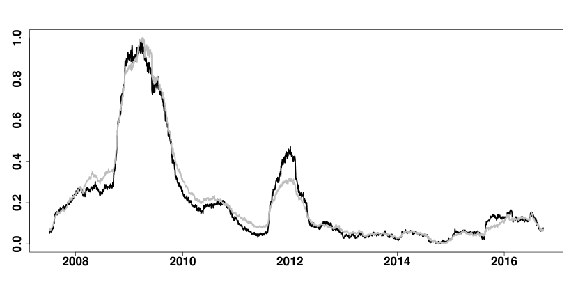
Figure 2: FRM with 100 firms (black) and FRM with 200 firms (grey), moving window size $n=126$.

 FRM_compare_nf

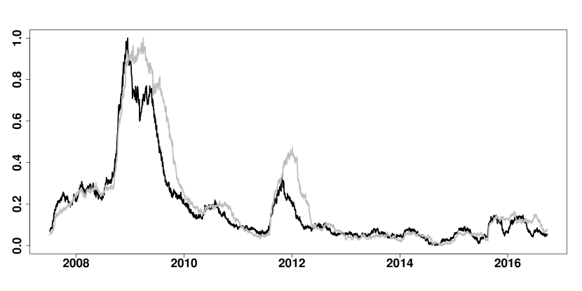
Figure 3: FRM with different moving window size, $n=63$ (black) and $n=126$ (grey), both series are scaled into the interval [0,1], from July 6, 2007 until September 23, 2016.

 FRM_compare_ws

We select six macro state variables to represent the general state of the economy: 1) the implied volatility index, VIX from Yahoo Finance; (2) the changes in the three-month Treasury bill rate from the Federal Reserve Bank of St. Louis; (3) the changes in the slope of the yield curve corresponding to the yield spread between the ten-year Treasury rate and the three-month bill rate from the Federal Reserve Bank of St. Louis; (4) the changes in the credit spread between BAA-rated bonds and the Treasury rate from the Federal Reserve Bank of St. Louis; (5) the daily S&P500 index returns from Yahoo Finance, and (6) the daily Dow Jones US Real Estate index returns from Yahoo Finance.

To compute the FRM we employ the tail parameter $\tau=0.05$. To find the a stable window size, $n$, we have to make a trade-off. We find that the lasso selection technique performs worse if the window size is too small. Since we use daily data, the moving window size should be larger than $50$, so that the estimation for each window is more precise. The results of using different window sizes (we have considered window sizes $n=63$ (one quarter) and $n=126$ (half a year)) are shown in Figure 3. The larger the window size, the more lagged, but also the smoother the plot is. Cross correlation can be used to determine the time delay of a time series, which we apply here for the estimate of the FRM with $n=63$ and the FRM with $n=126$. In Figure 4 and Table 1, the largest autocorrelation between FRM with $n=63$ and the lagged FRM with $n=126$ is $0.967$ from lag $-29$ to lag $-22$. We conclude that the FRM with $n=63$ leads the FRM $n=126$ by at least 22 periods. From all the preceding we set the moving window size to $n=63$.

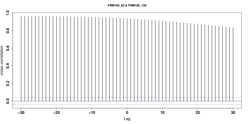
Figure 4: Cross correlation between FRM with $n=63$ and FRM with $n=126$, where the number of firms is 100.

 FRM_compare_ws

For each firm we have $2,386$ daily observations and $105$ covariates (99 firms and 6 macro-state variables). The FRM is the average of the $\lambda$’s computed from the 100 individual firms. The $\lambda$’s for the individual firms are more volatile and less smooth than the average over 100 firms and therefore more robust to reflect the impact from financial events on systemic risk. Figure 5 illustrates this by plotting the $\lambda$ of firm Wells Fargo (the largest firm by market capitalization) and the FRM.

Lag	-30	-29	-28	-27	-26	-25	-24	-23	-22	-21
Cross correlation	0.963	0.964	0.964	0.964	0.964	0.964	0.964	0.964	0.964	0.963

Table 1: Cross correlation between the estimates of the FRM with $n=63$ and FRM with $n=126$.

Figure 5: FRM (black) and $\lambda$ of Wells Fargo (grey), both series are scaled into interval [0,1], from April 5, 2007 until September 23, 2016.

 FRM_compare_of

3.2 Computational challenges

We wrote a script to automatically download the data from Yahoo Finance and Federal Reserve Bank of St. Louis. The R package quantmod is used. More details and the script are available from Quantnet ( FRM_download_data).

The $L_{1}$-norm quantile regression used to generate the $\lambda$ series is computationally intensive and therefore time-consuming, if applied sequentially for a large number of firms, see for instance the code from Quantnet ( FRM_lambda_series). Therefore, we consider parallel computing in R to reduce the computation time. R offers several algorithms for performance computing, such as lapply, mclapply, parLapply, for and foreach . For our purposes the foreach loops is the fastest solution, which we use for implementation.

We use the doParallel and foreach packages in R as developed and proposed by Calaway, Weston, Tenenbaum and Analytics (2015) and Calaway, Weston and Analytics (2015), see also Kane et al. (2013). Since we have 100 financial firms we use the foreach loops twice: the first loop is for the 100 financial firms with the second loop nested in the first loop to perform the moving window estimation. The speed of computation is increased considerably, the script is available from Quantnet:  FRM_parallel_compute.

Without the use of parallel computing, i.e. using a processor with four cores for each moving window, it requires around two minutes to generate the FRM estimate for one day. The Research Data Center (RDC) of Humboldt-Universität zu Berlin has provided access to their multi-core servers. Their servers have respectively 24, 32, and 40 cores. By using these servers combined with parallel computing, the average computation time is reduced approximately $12$ seconds to obtain a daily value for the FRM. The FRM webpage is updated weekly, which takes only 1 minute to generate the FRM series for five working days.

3.3 Visualization

To implement the visualization of the FRM, we use the JavaScript framework D3.js (or just D3 for Data-Driven Documents), which is a JavaScript library for producing dynamic, interactive data visualizations in web browsers. The QuantNetXploRer is a good example of D3 in power. More information about the D3 architecture, its various designs and the D3-based QuantNetXploRer can be found in Bostock et al. (2011) and Borke and Härdle (2017b).

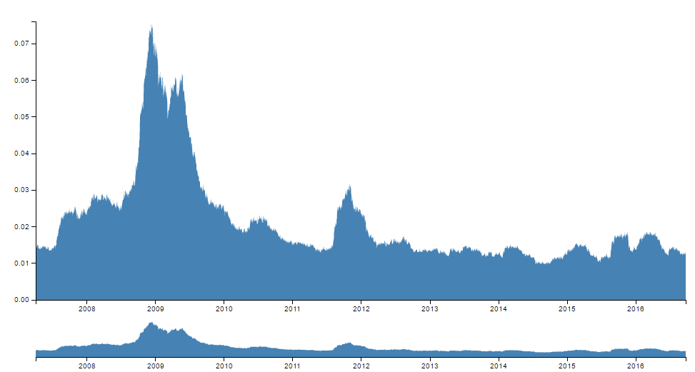
Figure 6: The graph of Financial Risk Meter (FRM).

 FRM_parallel_compute

Figure 6 illustrates the D3-based FRM visualization, and more examples e.g. for Asia, Europe are available on Althof et al. (2019).

3.3.1 Descriptive statistics

Figure 6 shows the FRM series from April 5, 2007 through September 23, 2016. The FRM has no theoretical upper bound. In the time frame under consideration, the maximum value is $0.075$, which occurred on December 15, 2008 and the mean value is $0.021$. We observe several peaks in the FRM series, which correspond to crises and other events in these periods. Two peaks correspond to the financial crises in 2008 and 2010. The peak in the first quarter of 2009 is at the height of the Great Recession: 800 thousand jobs were lost and the unemployment rate rose to $7.8\%$ in the US, which was the highest since June 1992. Another peak around the fourth quarter of 2011 coincides with the decline in stock markets in August 2011, which was due to fears of contagion of the European sovereign debt crisis to Spain and Italy.

Therefore one may state that the peaks of FRM series identify financial events and their impact on financial and systemic risk. The minimum of the FRM series in the time period under consideration is observed in August 26, 2014, with a value of $0.009$. This was a relatively stable period.

3.3.2 Risk levels

For convenience and following the color scheme of US homeland security office we divide risk into five levels with different classifications and colors. The levels of risk are defined as different intervals of ratios for the FRM. These ratios are computed based on the past values of the FRM. As shown in Figure 7, we have five levels of risk with five color codes. The current risk level is determined by the ratio based on all past FRM observations into which the current $\lambda$ falls. Table 2 presents the risk levels as well as the colors, descriptions and ratios of the risk levels.

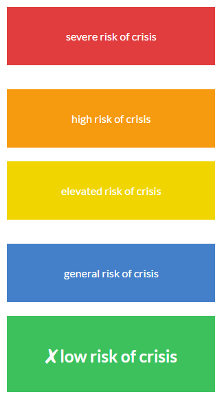
Figure 7: Risk levels of FRM

Color	Risk level description	FRM ratio
Green	Low risk of crisis in the financial market.	$<$20
	The incidence of a crisis is less likely than usual.
Blue	General risk of crisis in the financial market.	20-40
	There is no specific risk of a crisis.
Yellow	Elevated risk of crisis in the financial market.	40-60
	The incidence of a crisis is somewhat higher than usual.
Orange	High risk of crisis in the financial market.	60-80
	A crisis might occur very soon.
Red	Severe risk of a crisis in the financial market.	$>$80
	A financial crisis is imminent or happening right now.

Table 2: Risk levels, color codes and ratios for FRM

As an example, on September 23, 2016 the value of FRM was $0.013$. Since the maximum of FRM series up to that date was $0.075$, the ratio of this risk measure on September 23, 2016 was $17.3\%$. Since this is less than the 20%-ratio, we classify the risk on that day as low risk of crisis in the financial market with color green. On the website the current risk level is marked with a cross as shown in Figure 7 for this example.

4 Causality of FRM and other systemic risk measures

Zbonakova et al. (2017) analyze the factors affecting the value of $\lambda$ and summarize that $\lambda$ depends on three major factors: the variance of the error term, the correlation structure of the covariates and the number of non-zero coefficients of the model. Since high volatility indicates high risk in finance and the number of non-zero coefficients is related to the connectedness of the financial firms, they provide more theoretical evidence for the FRM as a risk measure. In their application, they find a co-integration relationship between $\hat{\lambda}$ and other systemic risk measures. We extend their idea and use Granger causality analysis to validate FRM. We select three measures: VIX (see Hallett; 2009), SRISK (see Brownlees and Engle; 2016) as well as the Google trends of the key word "financial crisis" (see Preis et al.; 2013).

For the causality analysis we first need to introduce the Vector Autoregression (VAR) model briefly. Lütkepohl (2005) proposes the VAR(P) model as follows:

$$y_{t}=\alpha+A_{1}y_{t-1}+A_{2}y_{t-2}+\cdots+A_{P}y_{t-P}+{\mathbf{u}_{t}},$$ (3)

where $y_{t}\stackrel{{\scriptstyle def}}{{=}}(y_{1t},\ldots,y_{Kt})^{\top}$, $A_{i}$ are fixed ($K\times K$) coefficient matrices, $\mathbf{u}_{t}$ is a $K$ dimensional process. The coefficients could be estimated by applying multivariate least squares estimation. In order to perform the Granger causality test, the vector of endogenous variables $y_{t}$ is split into two subvectors $y_{1t}$ and $y_{2t}$ with dimensions $(K_{1}\times 1)$ and $(K_{2}\times 1)$ and $K=K_{1}+K_{2}$. Then the VAR(P) model can be rewritten as follows:

$$y_{t} = \left(\begin{array}[]{c}y_{1t}\\ y_{2t}\\ \end{array}\right)=\left(\begin{array}[]{c}\alpha_{1}\\ \alpha_{2}\\ \end{array}\right)+\left(\begin{array}[]{cc}A_{11,1}&A_{12,1}\\ A_{21,1}&A_{22,1}\\ \end{array}\right)\left(\begin{array}[]{c}y_{1,{t-1}}\\ y_{2,{t-1}}\\ \end{array}\right)+\cdots$$ (19)

$$\hskip 86.11084pt+\left(\begin{array}[]{cc}A_{11,P}&A_{12,P}\\ A_{21,P}&A_{22,P}\\ \end{array}\right)\left(\begin{array}[]{c}y_{1,{t-P}}\\ y_{2,{t-P}}\\ \end{array}\right)+\left(\begin{array}[]{c}u_{1t}\\ u_{2t}\\ \end{array}\right)$$

The null hypothesis of the Granger causality test is that the subvector $y_{1t}$ does not Granger-cause $y_{2t}$, which is defined as $A_{21,i}=0$ for $i=1,2,\ldots,P$. The alternative hypothesis states that the subvector $y_{1t}$ Granger-causes $y_{2t}$ and is defined as: $\exists\,A_{21,i}\neq 0$ for $i=1,2,\ldots,P$. The test statistic follows an $F$ distributions with $PK_{1}K_{2}$ and $KJ-n^{*}$ degrees of freedom, where $J$ is the sample size and $n^{*}$ equals the total number of parameters in the above VAR(P) model.

4.1 FRM versus VIX

The VIX series is often addressed as a “fear index” and can be interpreted as a measure for systemic risk (Hallett; 2009). For reasons of comparability, we standardize these two series by setting the lowest value in the sample to zero and the highest to one. Figure 8 plots the standardized FRM series (thick black line) and the VIX series (thin red line). The plot shows that both indicators move in the same direction, with the VIX series a little more volatile. We also get some evidence of some financial events by observing the corresponding volatility levels of the FRM and VIX. For example, in the end of 2008 there is a sharp upward trend of FRM, whereas the upward trends dominates VIX as well, which corresponds to the bankruptcy of Lehman Brothers on September 15, 2008. Both FRM and VIX have higher values between 2008 and 2010, which corresponds to the time period of the financial crises. After 2013 the values of FRM are relative stable at a low level, while there is similar pattern of VIX, which shows signs of the slow recovery of the global economy from the recession.

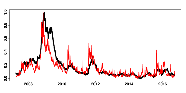
Figure 8: Scaled FRM (thick black line) and VIX (thin red line)

 FRM_VIX

Before we perform the Granger causality test, we test for stationarity of both time series with the Augmented Dickey-Fuller (ADF) test. The results of the test are shown in Table 3. For the FRM series, the $p$ value is larger than $0.05$, so we cannot reject the null hypothesis, i.e. the FRM series may have a unit root and may be non-stationary. We reject the null hypothesis for the VIX series with a $p$ value smaller than $0.05$ and conclude that the VIX series is stationary. We do not need to consider the co-integration problem, since only if both series are non-stationary, we should take into account the co-integration. There is a trade-off between using the original data and the transformed (differenced) data to find the causality relationship. Sims (1980) prefers to use the original data. He argues that VAR with non-stationary variables may provide important insights, if one is interested in the nature of relationships between variables. Brooks (2014) also states that differencing will destroy information on any long-run relationships between the series. However, other people argue that the original non-stationary data might lead to untrusted estimation, see Yule (1926) and Granger and Newbold (1974). In our case, we consider both the original data and transformed data.

Series	$p$ values
FRM	$0.28$
VIX	0.01
DFRM	$0.01$

Table 3: $p$ values of ADF test for stationarity

 FRM_VIX

Model	AIC	HQ	SC	FPE
FRM and VIX	20	$3$	$3$	20
DFRM and VIX	19	$8$	$5$	19

Table 4: Suggested order for VAR process by different criteria

Model	Order VAR	PT (asymptotic)	PT (adjusted)	BG	ES
FRM and VIX	3	$<2.2\times 10^{-16}$	$<2.2\times 10^{-16}$	$1.1\times 10^{-07}$	$1.0\times 10^{-07}$
	11	$2.5\times 10^{-07}$	$2.0\times 10^{-07}$	$1.6\times 10^{-01}$	$1.7\times 10^{-01}$
	20	$<2.2\times 10^{-16}$	$<2.2\times 10^{-16}$	$3.1\times 10^{-08}$	$4.1\times 10^{-08}$
DFRM and VIX	5	$2.2\times 10^{-16}$	$2.2\times 10^{-16}$	$3.2\times 10^{-08}$	$3.1\times 10^{-08}$
	8	$6.7\times 10^{-12}$	$4.9\times 10^{-12}$	$1.4\times 10^{-06}$	$1.5\times 10^{-06}$
	11	$2.3\times 10^{-09}$	$1.8\times 10^{-09}$	$1.5\times 10^{-03}$	$1.7\times 10^{-03}$
	19	$1.7\times 10^{-03}$	$1.6\times 10^{-03}$	$5.5\times 10^{-08}$	$7.2\times 10^{-08}$

Table 5: $p$ values of model selection tests

Cause	Effect	$p$ values
FRM	VIX	$4.0\times 10^{-08}$
VIX	FRM	$6.1\times 10^{-11}$
DFRM	VIX	$6.6\times 10^{-11}$
VIX	DFRM	$8.7\times 10^{-13}$

Table 6: $p$ values of Granger causality test

 FRM_VIX

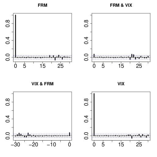
Figure 9: Autoregression functions of FRM and VIX

 FRM_VIX

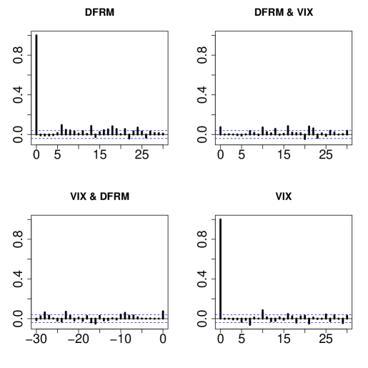
Figure 10: Autoregression functions of DFRM and VIX

 FRM_VIX

Firstly, we consider the original data. We choose the VAR order according to four criteria: the Akaike information criterion (AIC), the Hannan-Quinn information criterion

(HQ), the Schwarz criterion (SC) and the Prediction Error Criterion (FPE), see Table 4. While HQ and SC suggest an order 3 VAR process, AIC and FPE suggest an order 20 process. We fit both VAR models with order 3 and order 20. Next, we check the autocorrelation of the residuals to decide the optimal order. Four tests are carried out: the asymptotic Portmanteau Test, the adjusted Portmanteau Test, the Breusch-Godfrey LM test and the Edgerton-Shukur F test. The null hypothesis of these tests is that there is no first order autocorrelation among residuals. Choosing order 3 and 20 leads to the rejection of all these tests (cf. Table 5). Subsequently we try the other orders and find that with order 11 both the Breusch-Godfrey LM test and the Edgerton-Shukur F tests are passed. Therefore, we select order 11. The autocorrelation function of the residuals is plotted in Figure 9. Table 6 shows the results of the Granger causality test. All $p$ values are smaller than $0.05$ which indicates that the null hypothesis is rejected. Therefore, FRM Granger causes VIX, and also VIX Granger causes FRM.

Next, we consider the transformed series. Since FRM is non-stationary, we take the first difference. The transformed series is called as DFRM. In Table 3 we see that DFRM is stationary. Then the same procedure as before is performed. While HQ suggests an order 8 process, SC suggest an order 5, and AIC and FPE both suggest an order 19 (cf. Table 4). After checking the four tests for autocorrelation of the residuals, we conclude that the optimal order is 19. Although it does not pass the autocorrelation test, the $p$ value is close to the critical value $0.05$, and the autocorrelation function confirms this result (cf. Table 5 and Figure 10). The result of the Granger causality test is summarized in Table 6. We find that all $p$ values are significantly smaller than $0.05$, which indicates that the null hypothesis is rejected. Therefore we conclude that DFRM Granger causes VIX, and also VIX Granger causes DFRM.

4.2 FRM versus SRISK

SRISK is a macro-finance measure of systemic risk (Acharya et al.; 2012; Brownlees and Engle; 2016). Our data on SRISK for the US are obtained from V-Lab . We also standardize SRISK, so that both series are comparable on the same scale. Figure 11 plots the standardized FRM series (thick black line) and the SRISK series (thin blue line). We see that there is a peak in the first quarter of 2008 for SRISK, but afterwards FRM and SRISK have similar patterns. Especially during the beginning of 2010 and the beginning of 2012, the two series have a similar shape.

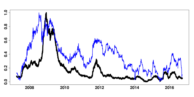
Figure 11: Scaled FRM (thick black line) and SRISK (thin blue line)

 FRM_SRISK

Variables	p-values
FRM	$0.48$
SRISK	0.10

Table 7: $p$ values of ADF test for stationarity for FRM and SRISK

Explanatory (Cause)	Response (Effect)	Value of test-statistic	Critical value at 5%
FRM	SRISK	-3.1	-1.95
SRISK	FRM	-2.7	-1.95

Table 8: Results of Engle Granger 2-step co-integration test

 FRM_SRISK

We perform the same procedure as in section 4.1. The results of the ADF test for the SRISK series in Table 7 show that the series is non-stationary. Since the FRM series is neither stationary, we consider the co-integration of them. From Granger (1988) we know that if both series are co-integrated, then there must be Granger causality between them in at least one way. We perform the Engle Granger 2-step test for co-integration, which is suitable for bivariate time series. In the first step, the linear regression of FRM on SRISK is carried out, i.e. FRM is the explanatory variable and SRISK the response variable. In the second step, we test the residuals of the aforementioned linear regression. If these residuals are stationary, then there is co-integration of FRM and SRISK. The null hypothesis of this test is that the residuals are non-stationary. The result of this test are summarized in Table 8. We conclude that FRM and SRISK are co-integrated, in other words, FRM Granger causes SRISK. If we regress SRISK on FRM, i.e. SRISK is the explanatory variable and FRM the response variable, we also conclude that SRISK and FRM are co-integrated, which indicates that SRISK Granger causes FRM. We thus conclude that there is mutual causality between FRM and SRISK.

4.3 FRM versus Google Trends

Finally, we analyze the relationship between FRM and Google Trends (GT) for the keyword "financial crisis". Google Trends provides data on the search volume of particular words and phrases relative to the total search volume. This can be disaggregated by countries. If a keyword is more frequently searched for, this might indicate a particular interest. Preis et al. (2013) analyzed the data related to finance from Google Trends, and find that Google Trends data did not only reflect the current state of the stock markets, but may have also been able to forecast certain future trends. We use Google Trends for the keyword "financial crisis", assuming that more people will search for this term if they feel the risk for a financial crisis is high. The Google Trends data are weekly data. To allow for comparison with the FRM we apply cubic interpolation to estimate daily data from the weekly Google Trends series. This series is compared with the daily FRM series. Figure 12 plots both the daily FRM series as well as the cubic interpolated Google Trends daily series. Both series are standardized to the interval zero-one for comparison. We observe some co-movement between both series, but no continuous superiority of the Google Trends above FRM.

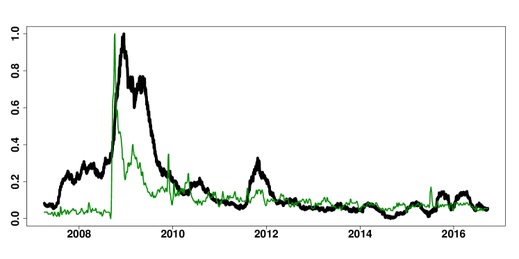
Figure 12: Scaled FRM (thick black line) and Google Trends (thin green line)

 FRM_GT

The ADF test shows that the GT series is stationary (cf. Table 9). We perform two tests for the relationship between the two series. Firstly, we consider the original data of FRM, then we consider the transformed data. We perform four criteria to find the optimal order of VAR model. As the results in Table 10 show, all the criteria suggest an order 20 VAR process. Therefore, we apply an order 20 VAR model. Next, the autocorrelation of the residuals is tested. Although none of the tests can be passed (cf. Table 11), we have no better choice for the order than 20. The autocorrelation function of residuals are plotted in Figure 13. Table 12 shows the results of the Granger causality test. All $p$ values are significantly smaller than $0.05$, which indicates that the null hypothesis is rejected. Therefore, FRM Granger causes GT, and GT Granger causes FRM.

For the first differenced FRM, i.e. DFRM, the same procedure is used. In Table 10 all the criteria suggest an order 20 VAR process. The result of the autocorrelation tests are presented in Table 10. Although none of the tests is passed, we still use order 20. The autocorrelation function of the residuals is shown in Figure 14. Table 12 shows the results of the Granger causality test. All $p$ values are significantly smaller than $0.05$, which indicates that the null hypothesis is rejected. Therefore, DFRM Granger causes GT, and GT Granger causes DFRM.

Variables	p-values
FRM	$0.48$
GT	0.01
DFRM	$0.01$

Table 9: $p$ values of ADF test for stationarity for FRM and GT

Model	AIC	HQ	SC	FPE
FRM and GT	20	$20$	$20$	20
DFRM and GT	20	$20$	$20$	20

Table 10: Suggested order for VAR process by different criteria

Model	Order	PT (asymptotic)	PT (adjusted)	BG	ES
FRM and GT	20	$<2.2\times 10^{-16}$	$<2.2\times 10^{-16}$	$<2.2\times 10^{-16}$	$<2.2\times 10^{-16}$
DFRM and GT	20	$<2.2\times 10^{-16}$	$<2.2\times 10^{-16}$	$<2.2\times 10^{-16}$	$<2.2\times 10^{-16}$

Table 11: $p$ values of model selection tests

Cause	Effect	p-values
FRM	GT	$1.1\times 10^{-10}$
GT	FRM	$2.1\times 10^{-12}$
DFRM	GT	$6.8\times 10^{-11}$
GT	DFRM	$4.1\times 10^{-10}$

Table 12: $p$ values of Granger causality test

 FRM_GT

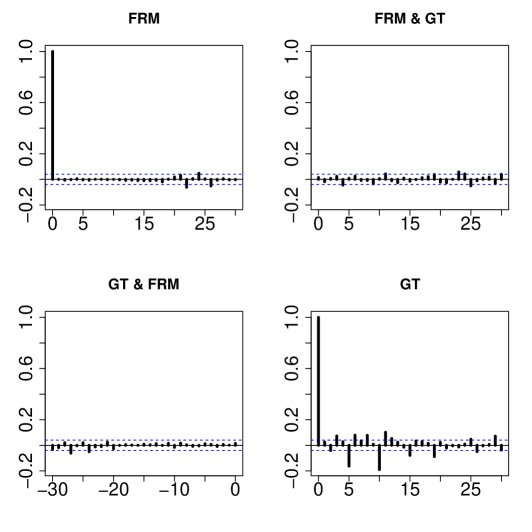
Figure 13: Autoregression functions of FRM and GT

 FRM_GT

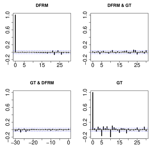
Figure 14: Autoregression functions of DFRM and GT

 FRM_GT

5 Conclusion

In this paper we propose and develop an AI based measure for systemic risk in financial markets: the Financial Risk Meter (FRM). The FRM is a measure for systemic risk based on the penalty term $\lambda$ of the linear quantile lasso regression, which is defined as the average of the $\lambda$ series over the 100 largest US publicly traded financial institutions. The implementation is carried out by using parallel computing. The risk levels are classified by five levels. The empirical result shows that our Financial Risk Meter can be a good indicator for trends in systemic risk. Compared with other systemic risk measures, such as VIX, SRISK, Google Trends with the keyword “financial crisis”, we find that the FRM and VIX, FRM and SRISK, FRM and GT mutually granger cause one another, which means that our FRM is a good measure of systemic risk for the US financial market. All the codes of FRM are published on www.quantlet.de with keyword  FRM. The R package RiskAnalytics (Borke; 2017b) is another tool with the purpose of integrating and facilitating the research, calculation and analysis methods around the FRM project (Borke; 2017a). The up-to-date FRM can be found on hu.berlin/frm.

6 Appendix: Financial Institutions

Table 13: The list of 100 financial companies used to estimate FRM in our sample.

WFC	Wells Fargo & Company	AON	Aon plc
JPM	J P Morgan Chase & Co	ALL	Allstate Corporation
BAC	Bank of America Corporation	BEN	Franklin Resources, Inc.
C	Citigroup Inc.	STI	SunTrust Banks, Inc.
AIG	American International Group, Inc.	MCO	Moody’s Corporation
GS	Goldman Sachs Group, Inc.	PGR	Progressive Corporation
USB	U.S. Bancorp	AMP	Ameriprise Financial Services, Inc.
AXP	American Express Company	AMTD	TD Ameritrade Holding Corporation
MS	Morgan Stanley	HIG	Hartford Financial Services Group, Inc.
BLK	BlackRock, Inc.	TROW	T. Rowe Price Group, Inc.
MET	MetLife, Inc.	NTRS	Northern Trust Corporation
PNC	PNC Financial Services Group, Inc. (The)	MTB	M&T Bank Corporation
BK	Bank Of New York Mellon Corporation (The)	FITB	Fifth Third Bancorp
SCHW	The Charles Schwab Corporation	IVZ	Invesco Plc
COF	Capital One Financial Corporation	L	Loews Corporation
PRU	Prudential Financial, Inc.	EFX	Equifax, Inc.
TRV	The Travelers Companies, Inc.	PFG	Principal Financial Group Inc
CME	CME Group Inc.	RF	Regions Financial Corporation
CB	Chubb Corporation	MKL	Markel Corporation
MMC	Marsh & McLennan Companies, Inc.	FNF	Fidelity National Financial, Inc.
BBT	BB&T Corporation	LNC	Lincoln National Corporation
ICE	Intercontinental Exchange Inc.	CBG	CBRE Group, Inc.
STT	State Street Corporation	KEY	KeyCorp
AFL	Aflac Incorporated	NDAQ	The NASDAQ OMX Group, Inc.
CINF	Cincinnati Financial Corporation	CACC	Credit Acceptance Corporation
CNA	CNA Financial Corporation	BRO	Brown & Brown, Inc.
HBAN	Huntington Bancshares Incorporated	ERIE	Erie Indemnity Company
SEIC	SEI Investments Company	OZRK	Bank of the Ozarks
ETFC	E*TRADE Financial Corporation	WTM	White Mountains Insurance Group, Ltd.
AMG	Affiliated Managers Group, Inc.	SNV	Synovus Financial Corp.
RJF	Raymond James Financial, Inc.	ISBC	Investors Bancorp, Inc.
UNM	Unum Group	MKTX	MarketAxess Holdings, Inc.
NYCB	New York Community Bancorp, Inc.	LM	Legg Mason, Inc.
Y	Alleghany Corporation	CBSH	Commerce Bancshares, Inc.
SBNY	Signature Bank	BOKF	BOK Financial Corporation
CMA	Comerica Incorporated	EEFT	Euronet Worldwide, Inc.
AJG	Arthur J. Gallagher & Co.	DNB	Dun & Bradstreet Corporation
TMK	Torchmark Corporation	WAL	Western Alliance Bancorporation
WRB	W.R. Berkley Corporation	EV	Eaton Vance Corporation
AFG	American Financial Group, Inc.	CFR	Cullen/Frost Bankers, Inc.
SIVB	SVB Financial Group	MORN	Morningstar, Inc.
EWBC	East West Bancorp, Inc.	THG	The Hanover Insurance Group, Inc.
ROL	Rollins, Inc.	UMPQ	Umpqua Holdings Corporation
ZION	Zions Bancorporation	CNO	CNO Financial Group, Inc.
AIZ	Assurant, Inc.	FHN	First Horizon National Corporation
PACW	PacWest Bancorp	WBS	Webster Financial Corporation
AFSI	AmTrust Financial Services, Inc.	PB	Prosperity Bancshares, Inc.
ORI	Old Republic International Corporation	PVTB	PrivateBancorp, Inc.
PBCT	People’s United Financial, Inc.	SEB	Seaboard Corporation
FCNCA	First Citizens BancShares, Inc.	MTG	MGIC Investment Corporation

References

- (1)
- Acharya et al. (2012) Acharya, V., Engle, R. and Richardson, M. (2012). Srisk as a macro-finance measure of systemic risk, https://bfi.uchicago.edu/sites/default/files/file_uploads/%234.pdf. Accessed: 2016-12-16.
- Adrian and Brunnermeier (2016) Adrian, T. and Brunnermeier, M. K. (2016). , American Economic Review 106(7): 1705–1741.
- Althof et al. (2019) Althof, M., Mihoci, A., Chen, C. Y.-H. and Härdle, W. K. (2019). financial risk meter, Empirical Economics, submitted .
- Borke (2017a) Borke, L. (2017a). RiskAnalytics: an R package for real time processing of Nasdaq and Yahoo finance data and parallelized quantile lasso regression methods, SFB 649 Discussion Paper 2017-006 . Humboldt Universität zu Berlin.
-
Borke (2017b)
Borke, L. (2017b).
RiskAnalytics: Real time processing of Nasdaq and Yahoo finance
data and parallelized quantile lasso regression methods.
R package version 0.2.0.
https://github.com/lborke/RiskAnalytics - Borke and Härdle (2017a) Borke, L. and Härdle, W. K. (2017a). GitHub API based QuantNet Mining infrastructure in R, SFB 649 Discussion Paper 2017-008 . Humboldt Universität zu Berlin.
- Borke and Härdle (2017b) Borke, L. and Härdle, W. K. (2017b). Q3-D3-LSA, in W. K. Härdle, H. H. Lu and X. Shen (eds), Handbook of Big data Analytics, Springer. doi: http://dx.doi.org/10.1007/978-3-319-18284-1.
- Bostock et al. (2011) Bostock, M., Ogievetsky, V. and Heer, J. (2011). D3 Data-Driven Documents, IEEE Transactions on Visualization and Computer Graphics 17(12): 2301–2309. doi: http://dx.doi.org/10.1109/TVCG.2011.185.
- Brooks (2014) Brooks, C. (2014). Introductory Econometrics for Finance, Cambridge University Press.
- Brownlees and Engle (2016) Brownlees, C. T. and Engle, R. F. (2016). : of , The Review of Financial Studies 30(1): 48–79. doi: https://doi.org/10.1093/rfs/hhw060.
-
Calaway, Weston and Analytics (2015)
Calaway, R., Weston, S. and Analytics, R. (2015).
foreach: Provides Foreach Looping Construct for R.
R package version 1.4.3.
https://CRAN.R-project.org/package=foreach -
Calaway, Weston, Tenenbaum and Analytics (2015)
Calaway, R., Weston, S., Tenenbaum, D. and Analytics, R.
(2015).
doParallel: Foreach Parallel Adaptor for the ’parallel’
Package.
R package version 1.0.10.
https://CRAN.R-project.org/package=doParallel - Fan et al. (2016) Fan, Y., Härdle, W. K., Wang, W. and Zhu, L. (2016). for the , Journal of Business economics and statistics .
-
Granger (1988)
Granger, C. (1988).
Some recent development in a concept of causality, Journal of
Econometrics 39(1): 199 – 211.
http://www.sciencedirect.com/science/article/pii/0304407688900450 - Granger and Newbold (1974) Granger, C. and Newbold, P. (1974). Spurious regressions in econometrics, Journal of Econometrics 2(2): 111–120.
- Hallett (2009) Hallett, N. (2009). Taming Risk–A guide for Traders, The Disciplined Trader.
- Härdle et al. (2016) Härdle, W., Wang, W. and Yu, L. (2016). : driven risk, Journal of Econometrics 192(2): 499–513. doi: http://dx.doi.org/10.1016/j.jeconom.2016.02.013.
- Hautsch et al. (2015) Hautsch, N., Schaumburg, J. and Schienle, M. (2015). Financial network systemic risk contributions, Review of Finance 19(2): 685–738.
-
Kane et al. (2013)
Kane, M., Emerson, J. and Weston, S. (2013).
Scalable strategies for computing with massive data, Journal of
Statistical Software 55(1): 1–19.
https://www.jstatsoft.org/index.php/jss/article/view/v055i14 - Li and Zhu (2008) Li, Y. and Zhu, J. (2008). L1-Norm Quantile Regression, Journal of Computational and Graphical Statistics 17(1).
- Lütkepohl (2005) Lütkepohl, H. (2005). New Introduction to Multiple Time Series Analysis, Springer.
- Preis et al. (2013) Preis, T., Moat, H. S. and Stanley, H. E. (2013). Quantifying Trading Behavior in Financial Markets Using Google Trends, Scientific Reports 3: 1684.
- Schwarcz (2008) Schwarcz, S. L. (2008). Systemic Risk, Georgetown Law Journal 97(1): 193–249.
- Sims (1980) Sims, C. A. (1980). Macroeconomics and reality, Econometrica 48(1): 1–48.
- Yuan (2006) Yuan, M. (2006). GACV for quantile smoothing splines, Computational statistics and data analysis 50(3): 813–829.
- Yule (1926) Yule, G. U. (1926). Why do we sometimes get nonsense-correlations between time-series?– study in sampling and the nature of time-series, Journal of the Royal Statistical Society 89(1): 1–63.
- Zbonakova et al. (2017) Zbonakova, L., Härdle, W. K. and Wang, W. (2017). Time Varying Quantile Lasso, in Applied Quantitative Finance (Härdle, Chen, Overbeck eds), Springer Verlag, pp. 331–353.