Dynamic mode decomposition to retrieve torsional Alfvén waves

1 Introduction

Signals arising from the deep interiors of planets are crucial sources of information about their physical conditions, information that is essentially inaccessible in situ. For instance, revealing the core dynamics at the centre of Earth is very limited: it is in principle inferred from the magnetic activity observed at/above the surface and there is difficulty in extracting details of its variations originated in the fluid core. Whilst satellite measurements have advanced over the last decades to find its ”rapid” dynamics of interannual changes the data investigation still largely relies on ground-based records over decades and longer (a recent review by [1] and references therein).Now the archaeo- or palaeo- magnetic datasets covered a wider area of the globe for longer intervals [2]; nonetheless their inhomogeneous coverage is inevitable.

An efficient technique to extract any intrinsic signals from the limited timeseries is therefore necessary to reveal the dynamics in the planetary interior and hence the dynamo. In addition to the classic Fourier transformation, earlier studies attempted the wavelet transformation [3] and the empirical mode decomposition (EMD) [4, 5] comprising cubic splines. Data-driven, modal analyses by the proper orthogonal decomposition (POD) –also known as principle component analysis (PCA) or empirical orthogonal functions (EOF)– have been made over geomagnetic datasets [6, 7]. POD was also used for model reduction of direct stochastic simulations for rotating fluids [8]. The method is however based on the energy ranking, with which any tiny, but physically relevant, signals may be lost. In many cases a POD mode comprises several modes which have different frequencies and growth rates.

Dynamic mode decomposition (DMD)[9] – an algorithm to approximate modes of the Koopman operator [10]– enables an extended, equation-free analysis to represent the temporal structures superior to POD, for example, by separating into individual mode of frequency and growth rate. The technique is now providing a powerful tool for diagnostics, future prediction, and control of multi-dimensional systems in a broad range of application areas, in addition to fluid dynamics (see [11] and references therein).

As observational exploration has developed, there is increasing evidence of magnetohydrodynamic (MHD) waves excited in Earth’s fluid core. A special class that is axisymmetric and quasi-geostrophic ($\mbox{\boldmath$\Omega$}\cdot\mbox{\boldmath$k$}\approx 0$ with $\Omega$ being the rotation axis and $k$ being the wavenumber vector) is called torsional Alfvén waves (TW): the inviscid, ideal wave for a Boussinesq/anelastic fluid is governed by

$$\frac{\partial^{2}}{\partial t^{2}}\frac{\langle u^{\prime}_{\phi}\rangle}{s}=\frac{1}{s^{3}h\langle\rho\rangle}\frac{\partial}{\partial s}\left(s^{3}h\langle\rho\rangle U_{\textrm{\scriptsize A}}^{2}\frac{\partial}{\partial s}\frac{\langle u^{\prime}_{\phi}\rangle}{s}\right)$$ (1)

[12, 13, 14, 15] where $s$ is the cylindrical radius, $h$ is the height from the equator, $\langle u^{\prime}_{\phi}\rangle$ is the axisymmetric geostrophic component of the fluctuating azimuthal velocity, $\langle\rho\rangle$ is the axisymmetric geostrophic component of the background density, and $U_{\textrm{\scriptsize A}}=\langle B_{s}\rangle/\sqrt{\mu\langle\rho\rangle}$ is the Alfvén speed with $\langle B_{s}\rangle$ being the equivalent component of the radial magnetic field and $\mu$ being the permeability. Although the excitation of these waves in the fluid core has been long a subject of debate the waves are believed to account for a several-year signal that was found in core flow models inverted from the observed geomagnetic secular variation [16, 1]. The signal was not very strong so that the identification required bandpass filterings. The equivalent periodicity in geomagnetic time-sequences was exploited by EMD and the Fourier analysis [5].

This MHD wave could reasonably be excited in other rapidly-rotating planets, such as in Jupiter’s metallic hydrogen region [15]. Here, unlike for a terrestrial planet, the disturbances may penetrate through the gaseous envelope to be visible near the surface. The cloud deck has been monitored by ground-based campaigns to find its long-term variation. Several-year periodicities in brightness were visualised by Lomb-Scargle and wavelet analyses at each latitude and were addressed by POD over the whole latitudes [17].

We here examine how DMD could help to identify signals of TW by means of spherical DNS for MHD fluids. For a first attempt we concentrate on a rather small set of data and on standard DMD.

2 A brief overview of DMD

We consider standard DMD [9], incorporating some recent updates [18, 19], in this study. We consider a data sequence $[\mbox{\boldmath$\psi$}_{0},\mbox{\boldmath$\psi$}_{1},...,\mbox{\boldmath$\psi$}_{N}]$ where $\mbox{\boldmath$\psi$}_{i}=\psi(x,i\Delta t)$ is a real vector with $N+1$ points in time $t$ sampled every $\Delta t$ and $M$ components in space $x$, $\psi_{i}\in\mathbb{R}^{M}$, with $M{\color[rgb]{0,0,0}>}N$. We then form two matrices:

$$\begin{split}\Psi_{0}&=[\mbox{\boldmath$\psi$}_{0}\;\mbox{\boldmath$\psi$}_{1}\;...\;\mbox{\boldmath$\psi$}_{N-1}]\in\mathbb{R}^{M\times N}\\ \textrm{and}\quad\Psi_{1}&=[\mbox{\boldmath$\psi$}_{1}\;\mbox{\boldmath$\psi$}_{2}\;...\;\mbox{\boldmath$\psi$}_{N}]\quad\in\mathbb{R}^{M\times N},\end{split}$$ (2)

and link the two so that the neighbouring snapshots can be expressed as a linear, discrete-time system:

$$\Psi_{1}=A\Psi_{0}\quad\textrm{where}\quad A\in\mathbb{R}^{M\times M}\;.$$ (3)

Given the $M$ eigensolutions of $A=\Psi_{1}\Psi_{0}^{\dagger}$ (where ^† denotes the pseudo inverse matrix), the data sequence may be represented by the linear combination of those modes (sometimes called exact DMD modes).

For a quite large set of data, which is the case of interest, we may seek an optimal representation $\widetilde{A}\in\mathbb{R}^{r\times r}$ of the matrix (with $r<M$) such that

$$A\approx U\widetilde{A}U^{\textrm{\scriptsize T}}\qquad\textrm{or}\qquad U^{\textrm{\scriptsize T}}AU\approx\widetilde{A}$$ (4)

where $U$ is obtained from an singular value decomposition of $\Psi_{0}$, i.e.

$$\Psi_{0}=U\Sigma V^{\textrm{\scriptsize T}}\;.$$ (5)

Here $r$ is the rank of $\Psi_{0}$, $\Sigma$ is an $r\times r$ diagonal matrix with diagonal entries $\sigma_{j}\geq 0$ ordering as $\sigma_{1}\geq\sigma_{2}\geq...\geq\sigma_{r}$,

$$\begin{split}U&=[\mbox{\boldmath$u$}_{1}\;\mbox{\boldmath$u$}_{2}\;...\mbox{\boldmath$u$}_{r}]\in\mathbb{R}^{M\times r},\\ \textrm{and}\quad V&=[\mbox{\boldmath$v$}_{1}\;\mbox{\boldmath$v$}_{2}\;...\mbox{\boldmath$v$}_{r}]\in\mathbb{R}^{N\times r}.\end{split}$$ (6)

Note $U$ contains the spatial structures (topos) whilst $V$ contains the temporal structures (chronos). Vectors $\mbox{\boldmath$u$}_{j}$ in $U$ may be regarded as POD modes of the dataset in $\Psi_{0}$, together with the singular values $\sigma_{j}$ describing the contained energy in descending order. The matrix $\widetilde{A}$ is obtained by minimising the Frobenius norm of the difference

$$||\Psi_{1}-A\Psi_{0}||^{2}_{\textrm{\scriptsize F}}\approx||\Psi_{1}-U\widetilde{A}\Sigma V^{\textrm{\scriptsize T}}||^{2}_{\textrm{\scriptsize F}}$$ (7)

to give

$$\widetilde{A}=U^{\textrm{\scriptsize T}}\Psi_{1}V\Sigma^{-1}.$$ (8)

When the $r$ eigenvalues ($\mu_{j}$) and eigenvectors ($\mbox{\boldmath$z$}_{j}$) of $\widetilde{A}$ are found, the original data at time $i\Delta t$ may be approximated as

$$\mbox{\boldmath$\psi$}_{i}\approx\sum_{j=1}^{r}U\mbox{\boldmath$y$}_{j}\;\mu_{j}^{i}\;\mbox{\boldmath$z$}_{j}^{\textrm{\scriptsize{\color[rgb]{0,0,0}H}}}\mbox{\boldmath$x$}_{0}\equiv\sum_{j=1}^{r}\mbox{\boldmath$\phi$}_{j}e^{\lambda_{j}t}\alpha_{j}\;.$$ (9)

Here the (projected) DMD eigenvalue is given by $\lambda_{j}=(\ln{\mu_{j}})/\Delta t$, its eigenfunction $\mbox{\boldmath$\phi$}_{j}=U\mbox{\boldmath$y$}_{j}$ with $\mbox{\boldmath$y$}_{j}$ satisfying $\mbox{\boldmath$z$}^{\textrm{\scriptsize{\color[rgb]{0,0,0}H}}}_{k}\mbox{\boldmath$y$}_{j}=\delta_{jk}$ (where the superscript ${}^{\textrm{\scriptsize H}}$ denotes the complex conjugate transpose), and its optimal amplitude $\alpha_{j}=\mbox{\boldmath$z$}_{j}^{\textrm{\scriptsize{\color[rgb]{0,0,0}H}}}\mbox{\boldmath$x$}_{0}$ with $\mbox{\boldmath$x$}_{0}$ being the initial data where $\mbox{\boldmath$x$}_{i+1}=\widetilde{A}\mbox{\boldmath$x$}_{i}$. The real and imaginary parts of $\lambda_{j}$ represent the growth rate and the frequency, respectively.

The optimal amplitude is determined so that the solutions should minimise

$$||\Psi_{0}-\Phi D_{\alpha}V_{\textrm{\scriptsize and}}||^{2}_{\textrm{\scriptsize F}}$$ (10)

where $\Phi=[\mbox{\boldmath$\phi$}_{1}\;\mbox{\boldmath$\phi$}_{2}\;...\mbox{\boldmath$\phi$}_{r}]\in{\color[rgb]{0,0,0}\mathbb{C}}^{M\times r}$, $D_{\alpha}$ is an $r\times r$ diagonal matrix with diagonal entries $\alpha_{j}$, and $\{V_{\textrm{\scriptsize and}}\}_{ji}=\mu_{j}^{i}\in{\color[rgb]{0,0,0}\mathbb{C}}^{r\times N}$. This may be rewritten as minimising

$$||\Sigma V^{\textrm{\scriptsize T}}-YD_{\alpha}V_{\textrm{\scriptsize and}}||^{2}_{\textrm{\scriptsize F}}\;,$$ (11)

where $\Phi=UY$, or minimising

$$J(\mbox{\boldmath$\alpha$})=\mbox{\boldmath$\alpha$}^{\textrm{\scriptsize{\color[rgb]{0,0,0}H}}}P\mbox{\boldmath$\alpha$}-q^{\textrm{\scriptsize{\color[rgb]{0,0,0}H}}}\mbox{\boldmath$\alpha$}-\mbox{\boldmath$\alpha$}^{\textrm{\scriptsize{\color[rgb]{0,0,0}H}}}q+s$$ (12)

where $\mbox{\boldmath$\alpha$}=[\alpha_{1}\;\alpha_{2}\;...\;\alpha_{r}]$, $P=(Y^{\textrm{\scriptsize{\color[rgb]{0,0,0}H}}}Y)\circ(\overline{V_{\textrm{\scriptsize and}}V_{\textrm{\scriptsize and}}^{\textrm{\scriptsize{\color[rgb]{0,0,0}H}}}})$, $q=\overline{\textrm{diag}(V_{\textrm{\scriptsize and}}V\Sigma^{\textrm{\scriptsize T}}Y)}$, and $s=\textrm{trace}(\Sigma^{\textrm{\scriptsize T}}\Sigma)$. Here the overbar denotes the complex conjugate, and $\circ$ represents the element-wise multiplication. By minimising $J(\mbox{\boldmath$\alpha$})$ the optimal vector of the DMD amplitude is obtained as

$$\mbox{\boldmath$\alpha$}=P^{-1}q\;.$$ (13)

In the analysis presented below, we quantify the accuracy of our decomposition in terms of the residual, (10) or (11), between the sampled and estimated data and also the performance of loss

$$\Pi_{\textrm{\scriptsize loss}}\equiv 100\sqrt{\frac{J(\mbox{\boldmath$\alpha$})}{J(\mbox{\boldmath$0$})}}$$ (14)

of the retained DMD modes. The efficiency of DMD can also be measured by the rank $r$ of the approximated matrix against $M$ for the sampled data. In addition, we check the singular values $\sigma_{j}$ to learn how many DMD (or POD) modes, out of the $r$ modes, will effectively approximate the data.

3 DMD of numerical data

We consider two types of numerical data which were obtained from 3D DNS of MHD fluids in rapidly rotating spherical shells: (i) Boussinesq convection permeated by a dipolar poloidal field (referred to as ’magnetoconvection’ hereafter) [14] and (ii) dynamos driven by anelastic convection incorporating a transition to the hydrodynamic envelope (’Jovian dynamo’) [20, 15]. The respective models were designed for Earth’s liquid iron core and Jupiter’s metallic/molecular hydrogen region, respectively. We note that the dynamo runs presented below yield self-generated magnetic fields dominated by an axial dipole. For both types of models, time and length are scaled, respectively, by magnetic diffusion time $\tau_{\textrm{\scriptsize m}}$ and by the radius $r_{\textrm{\scriptsize o}}$ of the outer shell in our simulations. This radius is identified the top of Earth’s core for the magnetoconvection cases, and about 0.96 of Jupiter’s nominal radius for the Jovian dynamo cases.

The original spherical data were converted to cylindrical coordinates $(s,\phi,z)$ and averaged over $\phi$ and $z$ to focus on the axisymmetric, geostrophic component $\langle u_{\phi}\rangle(s{\color[rgb]{0,0,0},t})$. In the all runs analysed below, the cylindrical fluctuations were previously identified as travelling or standing in $s$ and compared with the predicted phase/ray paths of TW [14, 15]: this may be regarded a local approach. An example for magnetoconvection is exhibited in figure 1. The contours of $\langle u_{\phi}\rangle$ in $s$-$t$ space show they mostly fluctuate outside the tangent cylinder (TC), located at $s/r_{\textrm{\scriptsize o}}=0.35$, and travel outwards. Below we shall examine if such TW identification in $\langle u_{\phi}\rangle$ is endorsed by DMD and TW normal modes: we call this a global approach, contrasting with the local one.

Figure 1: Axisymmetric, geostrophic zonal flow $\langle u_{\phi}\rangle$ in a magnetoconvection case 5E6P.1d [14]. In the northern hemisphere.

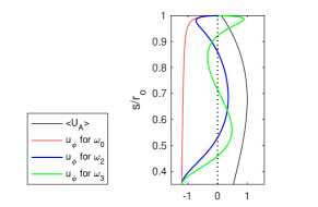
Figure 2: Profiles of the normalised Alfvén speed $U_{\textrm{\scriptsize A}}$ in run 5E6P.1d (black solid curve) and the eigenfunctions $\langle u^{\prime}_{\phi}\rangle$ of the 0th (red), 2nd (blue), and 3rd (green) TW normal modes outside the TC, provided a normalising factor at the inner bound.

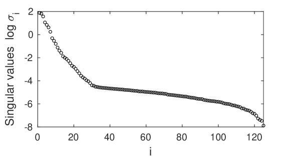
Figure 3: Singular values $\sigma_{j}$ in run 5E6P.1d.

3.1 Magnetoconvection

For a given Alfvén speed $U_{\textrm{\scriptsize A}}(s)$ and considering normal mode solutions ($\propto\exp{\textrm{i}\omega t}$), the TW equation (1) is solved outside the TC with the Matlab routine bvp4c. The number of grid points in $s$ is 500. The numerical code is benchmarked with solutions in a whole sphere [13, 21]: the first four eigenvalues for constant $U_{\textrm{\scriptsize A}}$ agree with those in the previous work to five decimal places. The first six eigenvalues (denoted by $\omega_{i}$) for the current problem, $U_{\textrm{\scriptsize A}}(s)$ obtained in the DNS, are found to be 77.2, 479, 731, 1000, 1275, and 1553, provided free-slip and no-slip conditions at $s/r_{\textrm{\scriptsize o}}=$ 0.3501 and 0.9999, respectively. Figure 2 demonstrates profiles of the assumed background profile $U_{\textrm{\scriptsize A}}(s)$ and selected eigenfunctions corresponding to the calculated eigenvalues. Here the $i$-th normal mode has $i$ nodes in $s$.

These TW normal modes are compared with DMD modes of the data $\langle u_{\phi}\rangle(s,t)$. The dataset has 127 grid points ($=M$) in $s$. The time sequence is 0.03 long with the sampling time $\Delta t=0.0001$, totaling up to 301 snapshots. Varying the number of analysed snapshots, we confirm 125 snapshots ($=N$) spanning over the window $0.0125\leq t/\tau_{\textrm{\scriptsize m}}<0.03$ (fig. 1), gives the rank $r=125$ and yield the residual (11) no greater than $10^{-6}$. Then $\Pi_{\textrm{\scriptsize loss}}$ (14) is diminished to less than 1% when 13 modes, out of the 125 DMD modes, are retained. The singular values $\sigma_{j}$ against $j$ are plotted in Figure 3 to show a sharp change at $j\approx 30$, beyond which the slope becomes gentle: this implies the low-dimensional structures are present. We also verify the projected DMD modes indeed pose a subset of the entire $M$ eigenmodes of $A$ (3), which are explicitly computed from the pseudo inverse matrix $\Psi_{0}^{\dagger}$. The eigenvalues, $\mu_{j}$, almost shape a circle in the complex plane (not shown).

Figure 4: DMD eigenvalues (top) and amplitude (bottom) in run 5E6P.1d. Modes 1, 2, 3, 4, and 5 are highlighted in red, blue, green, yellow, and magenta, respectively. The vertical dashed-dotted line labelled by $\omega_{i}$ indicates the frequency of the $i$-th TW normal mode.

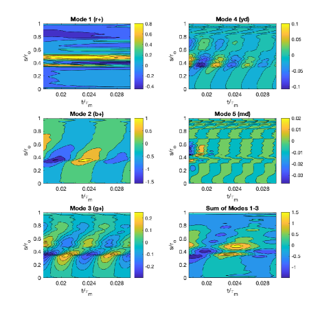
Figure 5: Spatiotemporal structures of DMD Modes 1-3 (from top to bottom) in run 5E6P.1d.

Figure 6: Profiles of DMD eigenfunctions of Modes 1 (red dashed curve), 2 (blue solid), and 3 (green solid) in run 5E6P.1d. Only outside the TC is shown.

The top panel of figure 4 displays the DMD eigenvalues, $\lambda_{j}=(\ln{\mu_{j}})/\Delta t$, of the data in frequency-growth rate space, whilst the amplitude $|\alpha_{j}|$ as a function of frequency is shown in the bottom panel. In order to seek a stable wave solution, we focus on modes that have nonzero frequencies in the range of the expected TW normal modes and small growth rates (or their quality factors, $Q=|\textrm{Im}(\lambda_{j})/2\textrm{Re}(\lambda_{j})|$, are no lower than unity). In both panels the frequencies $\omega_{i}$ of the first six TW modes are indicated by vertical dashed-dotted lines. The DMD extracts a non-oscillating component (zero frequency but growth rate $\approx 144$) and visualises several significant modes (which are highlighted in colour). The slowest mode (red; referred to as ‘Mode 1’) has a frequency close to $\omega_{0}$; the strongest is the second slowest mode (blue; ‘Mode 2’) of frequency $\approx 711.6$, close to $\omega_{2}$, and growth rate $\approx-60.9$. The third slowest mode (green; ‘Mode 3’) of frequency $\approx 1031$ and growth rate $\approx-35.5$ is close to $\omega_{3}$. The fourth mode (yellow; ‘Mode 4’) is found in between $\omega_{4}$ and $\omega_{5}$; there are more modes at higher frequency, including Mode 5 (magenta) beyond $\omega_{6}$.

We further exploit eigenfunctions of those DMD modes to distinguish the free oscillation. Figure 5 demonstrates contours of the selected DMD eigenfunctions, $\phi_{j}\exp{(\lambda_{j}t)}\alpha_{j}$, in $s$-$t$ space. Mode 1 appears to be quasi-steady and relevant in the neighbourhood of the TC. By contrast, Modes 2 and 3 exhibit a travelling nature towards the equator $s/r_{\textrm{\scriptsize o}}=1$. Their radial structures, $\phi_{j}$, are focused in figure 6. The red dashed curve confirms Mode 1 representing a TC-related mode. The other two curves show local maxima within the internal region: Mode 2 (blue solid curve) has a crest at $s/r_{\textrm{\scriptsize o}}\approx 0.55$ and crosses zeros at $s/r_{\textrm{\scriptsize o}}\approx 0.4$; Mode 3 (green) adds another trough at $s/r_{\textrm{\scriptsize o}}\approx 0.8$ and another crossing at $s/r_{\textrm{\scriptsize o}}\approx 0.65$. We therefore regard Modes 2 and 3 as related to an internal, free oscillation. Superposition of Modes 2 and 3 may represent the essential part of the wave motion (not shown). The two modes are retrieved even when the the number $N$ of analysed snapshots is limited to 75 (the window $0.0224\leq t/\tau_{\textrm{\scriptsize m}}<0.03$), whilst Mode 2 is only found to be a quasi-stationary wave with 25 snapshots ($0.0274\leq t/\tau_{\textrm{\scriptsize m}}<0.03$).

We however note that the number of the nodes does not completely match that expected from the 2nd or 3rd TW normal mode (fig. 2) despite the agreement in the frequency (fig. 4 top). Indeed, as $s/r_{\textrm{\scriptsize o}}\rightarrow 1$, the discrepancy in eigenfunction between the DMD and the TW normal modes becomes evident, indicating a damping occurs in the DNS. These could arise from the oversimplified model adopted for computing the TW normal modes: equation (1) clearly has a singularity at the outer bound. The inclusion of resistivity and/or viscosity may avoid the issue and reasonably influence details of the normal modes [22].

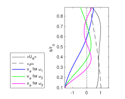
Figure 7: Profiles of the normalised Alfvén speed $U_{\textrm{\scriptsize A}}$ (black solid curve) and density $\langle\rho\rangle$ (black dashed) in a Jovian dynamo run E [20, 15], and the eigenfunctions $\langle u^{\prime}_{\phi}\rangle$ of the 1st (blue), 2nd (green), and 3rd (magenta) TW normal modes within the metallic region, provided a normalising factor at the inner bound.

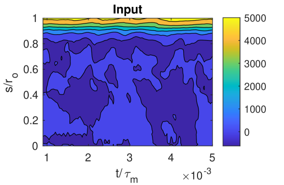
Figure 8: Axisymmetric, geostrophic zonal flow $\langle u_{\phi}\rangle$ in run E. In the northern hemisphere. The transition from the metallic to molecular region begins at about $s/r_{\textrm{\scriptsize o}}=0.885$-$0.94$.

3.2 Jovian dynamo

For the Jovian dynamo cases, a more complex structure of the background profiles is imposed (see details in [20]). The density and electrical conductivity vary with radius and drastically, but smoothly, decrease across a transition zone from the metallic hydrogen to the molecular hydrogen regions: the transition begins at about $s/r_{\textrm{\scriptsize o}}=0.885$-$0.944$. The TC attached to a rocky core is set to be at $s/r_{\textrm{\scriptsize o}}=0.0963$. When the simple TW model (1) is applied to the metallic region only ($0.0963\leq s/r_{\textrm{\scriptsize o}}\leq 0.885$) the normal modes for $U_{\textrm{\scriptsize A}}$ in the run and free slip boundary conditions have frequencies $\omega_{i}$, from the lowest, of 4804.8, 7716.6, 10492, 13308, 16179, and 19094. Their eigenfunctions are amplified with decreasing $s$, or the density (see selected ones in figure 7). Those precalculations would guide us to interpret DMD signals shown below; we however caution the current model omits any coupling between the metallic region and the overlying transition layer.

The analysed time sequence $\langle u_{\phi}\rangle$, as displayed in figure 8, has 87 points in $s$ and 72 snapshots in $t$, giving the rank $r={\color[rgb]{0,0,0}72}$ for DMD. For residual no greater than $10^{-7}$: $\Pi_{\textrm{\scriptsize loss}}<$ 9% with 60 modes. The singular value distribution $\sigma_{j}$ is now a rather smooth function of $j$ (not shown), indicating low-order models are relatively ineffective. The DMD distinguishes distinct modes in the vicinity of zero growth rate (fig. 9): in the frequency range up to $\omega_{6}$, there are 10 modes having the quality factor $Q$ higher than 5. In a similar manner to the magnetoconvection case earlier, we rank those DMD modes in their nonzero frequencies; ‘Mode 1’ for the slowest mode, ‘Mode 2’ for the secondly slowest mode, and so on. Only relevant modes are indicated by colour in the figure.

These modes may be classified as internal, transition-related, and coupled modes, depending on the radii at which the DMD eigenfunction has peaks, as follows. Their $s$-profiles and spatiotemporal structure are typically demonstrated in figures 10 and 11, respectively. Modes 1 and 4 (as indicated in red and yellow in fig. 9, respectively) have eigenfunctions maximised in the transition or poorly-conducting layer, i.e. $s/r_{\textrm{\scriptsize o}}\gtrsim 0.9$, while decaying (see the dashed-dotted curve in fig. 10 and the top panel in fig. 11 for Mode 1): we realise them transition-related modes. Modes 2 (blue) and 3 (green) are classed coupled modes: their eigenfunctions of both are largest at $s/r_{\textrm{\scriptsize o}}\approx 0.86$, near the lower bound of the transition zone, and notable at either larger and smaller radii (the blue dashed curve in fig. 10 for Mode 2). Interestingly those coupled modes appear to propagate from the radius both towards the deeper interior and towards the poorly conducting layer (the middle panel in fig. 11 for Mode 3). This could be interpreted as waves being reflected off and partially transmitted through the transition interface: the presence of a conductivity jump may give rise to reflections and transmissions of MHD waves [15]. Modes classed as internal include Modes 5 (magenta) and 8 (cyan), for which the eigenfunction is suppressed when $s/r_{\textrm{\scriptsize o}}\gtrsim 0.94$ but has peaks within the metallic region (the magenta and cyan solid curves in fig. 10): they reveal quasi-stationary standing waves, or oscillations (the bottom panel of fig. 11 for Mode 5). We also remark their frequencies almost match $\omega_{3}$ and $\omega_{5}$ of the free TW normal modes (fig. 9); details of the radial profile cannot be met perfectly. This, again, highlights the need for better understanding of the TW eigenvalue problem in more realistic situations.

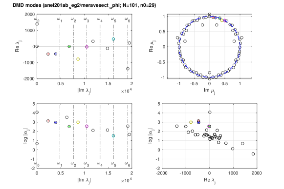
Figure 9: DMD eigenvalues (top) and amplitude (bottom) in run E. Modes 1, 2, 3, 4, 5, and 8 are indicated in red, blue, green, yellow, magenta, and cyan, respectively. The vertical dashed-dotted line labelled by $\omega_{i}$ indicates the frequency of the $i$-th TW normal mode in the metallic region.

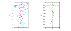
Figure 10: Profiles of selected DMD eigenfunctions in run E. The red dashed-dotted, blue dashed, magenta solid, and cyan solid curves represent the ones for Mode 1, 2, 5, and 8, respectively. The horizontal dotted lines indicate the radii $s/r_{\textrm{\scriptsize o}}=$ 0.885 and 0.94. Only outside the TC is shown.

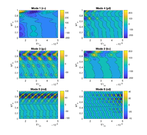
Figure 11: Spatiotemporal structures of DMD Modes 1, 3, and 5 (from top to bottom) in run E.

4 Summary

We have demonstrated the standard DMD of DNS data for rotating MHD convection and dynamos, in comparison with normal modes computed with the simple, diffusionless TW models. The methodology provides us with a global, but straightforward, approach to characterise MHD wave excited in the deep interiors of planets, for which available data is still limited. We will further extend our exploration to the data accessible at the surface.

References

- [1] Gillet, N., ”Spatial and temporal changes of the geomagnetic field: Insights from forward and inverse core field models,” arXiv: 1902.08098v1 (2019).
- [2] Nilsson, A., Holme, R., Korte, M., Suttie, N., and Hill, M., ”Reconstructing Holocene geomagnetic field variation: new methods, models and implications,” Geophys. J. Int., 198 (2014), pp. 229-248.
- [3] Alexandrescu, M., Gibert, D., Hulot, G., Le Mouël, J.-L., and Saracco, G., ”Detection of geomagnetic jerks using wavelet analysis,” J. Geophys. Res., 100 (1995), pp. 12557-12572.
- [4] Roberts, P.H., Yu, Z.J., and Russell, C.T., ”On the 60-year signal from the core,” Geophys. Astrophys. Fluid Dyn., 101 (2007), pp. 11-35.
- [5] Silva, L., Jackson, L., and Mound, J., ”Assessing the importance and expression of the 6 year geomagnetic oscillation,” J. Geophys. Res., 117 (2012), B10101 (9pp).
- [6] Chulliat, A. and Maus, S., ”Geomagnetic secular acceleration, jerks, and a localized standing wave at the core surface from 2000 to 2010,” J. Geophys. Res. Solid Earth, 119 (2014), pp. 1531-1543.
- [7] Domingos, J., Pais, M.A., Jault, D., and Mandea, M., ”Temporal resolution of internal magnetic field modes from satellite data,” Earth Planet. Space, 71 (2019), 2 (17pp).
- [8] Allawala, A., Tobias, S.M., and Marston, J.B., ”Dimensional reduction of direct statistical simulation,” arXiv: 1708.07805v2 (2018).
- [9] Schmid, P.J., ”Dynamic mode decomposition of numerical and experimental data,” J. Fluid Mech., 656 (2010) pp. 5-28.
- [10] Rowley, C.W., Mezić, I., Bagheri, S., Schlatter, P., and Henningson, D.S., ”Spectral analysis of nonlinear flows,” J. Fluid Mech., 641 (2009), pp. 115-127.
- [11] Kutz, J.N., Brunton, S.L., Brunton, B.W., and Proctor, J.L., ”Dynamoc Mode Decomposition: Data-Driven Modeling of Complex Systems,” 1st edition (2016), 234pp. SIAM: Philadelphia.
- [12] Braginsky, S.I., ”Torsional magnetohydrodynamic vibrations in the Earth’s core and variations in day length,” Geomag. Aeron., 10 (1970), pp. 1-8.
- [13] Roberts, P.H. and Aurnou, J.M., ”On the theory of core-mantle coupling,” Geophys. Astrophys. Fluid Dyn., 106 (2012), pp. 157-230.
- [14] Teed, R.J., Jones, C.A., and Tobias, S.M., ”The transition to Earth-like torsional oscillations in magnetoconvection simulations,” Earth Planet. Sci. Lett., 419 (2015), pp. 22-31.
- [15] Hori, K., Teed, R.J., and Jones, C.A., ”Anelastic torsional oscillations in Jupiter’s metallic hydrogen region,” Earth Planet. Sci. Lett., 519 (2019), pp. 50-60.
- [16] Gillet, N., Jault, D., Canet, E., and Fournier, A., ”Fast torsional waves and strong magnetic field within the Earth’s core,” Nature, 465 (2010), pp. 74-77.
- [17] Antuñano, A., Fletcher, L.N., Orton, G.S., Melin, H., Milan, S., Rogers, J., Greathouse, T., Harrington, J., Donnelly, P.T., and Giles, R., ”Jupiter’s atmospheric variability from long-term ground-based observations at 5m,” Astron. J., 158 (2019), 130 (28pp).
- [18] Jovanović, M.R., Schmid, P.J., and Nichols, J.W., ”Sparsity-promoting dynamic mode decomposition,” Phys. Fluids, 26 (2014), 024103 (22pp).
- [19] Horn, S. and Schmid, P.J., ”Prograde, retrograde, and oscillatory modes in rotating Rayleigh-Bénard convection,” J. Fluid Mech., 831 (2017), pp. 182-211.
- [20] Jones, C.A., ”A dynamo model of Jupiter’s magnetic field,” Icarus, 241 (2014), pp. 148-159.
- [21] Maffei, S. and Jackson, A., ”Propagation and reflection of diffusionless torsional waves in a sphere,” Geophys. J. Int., 204 (2016), pp. 1477-1489.
- [22] Mound, J. and Buffett, B., ”Viscosity of the Earth’s fluid core and torsional oscillations,” J. Geophys. Res., 112 (2007), B05402 (14pp).