A Weighted Quiver Kernel using Functor Homology

Abstract

In this paper, we propose a new homological method to study weighted directed networks. Our model of such networks is a directed graph $Q$ equipped with a weight function $w$ on the set $Q_{1}$ of arrows in $Q$. We require that the range $W$ of our weight function is equipped with an addition or a multiplication, i.e. $W$ is a monoid in the mathematical terminology. When $W$ is equipped with a representation on a vector space $M$, the standard method of homological algebra allows us to define the homology groups $H_{*}(Q,w;M)$.

It is known that when $Q$ has no oriented cycles, $H_{n}(Q,w;M)=0$ for $n\geq 2$ and $H_{1}(Q,w;M)$ can be easily computed. This fact allows us to define a new graph kernel for weighted directed graphs. We made two sample computations with real data and found that our method is practically applicable.

1 Introduction

Graphs and quivers (directed graphs) are ubiquitous in mathematical sciences. In many applications, vertices or edges of graphs and quivers are labeled and have costs associated with them, also called weights. In this paper, we are interested in edge-weighted quivers. These weights are not restricted to just scalar values, but can also represent much more complex and richer relations between the nodes of an edge by modeling them as label sets or a function of several variables.

Such weighted quivers arise frequently when modeling real-world applications, especially where the relationships among objects play an important role. Below are a few applications of weighted quivers that cover wide and diverse fields:

• Physics: weighted quivers are used to represent atomic structures, where an atom is depicted as a vertex and the interactive forces between the atoms (i.e., vertices) are shown as directed edges between pairs of vertices. The edge weights here can model the strength of interaction between two vertices. Note that such a weighted quiver also accepts multiple edges between the same pair of vertices, where each edge potentially represents a different type of interactive force.

• Chemistry: weighted quivers model molecular structures, where the vertices and the edges represent atoms and the chemical bonds between them, respectively. The edge weights contain information such as the bond angles, the magnitude of electrostatic force of attraction, polarity of the bonds, etc.

• Neuroscience: weighted quivers can represent a functional model of the brain, where vertices represent regions of the brain and the edges represent the connections or communication pathways between them. The edge weights can represent similarity between two brain signals at the vertices, information propagated between the vertices via the edge, etc.

• World Wide Web (WWW): weighted quivers represent the interconnections between documents on the web, where web documents are shown as vertices and edges represent the references between them. An edge weight in this instance could signify the number of times the source vertex referenced the target vertex, or how many web links they share in common etc.

We focus our attention to implementing a kernel method in the study of such weighted networks. Recall that, given a family of graphs $\mathcal{G}$, a graph kernel on $\mathcal{G}$ is a function $k:\mathcal{G}\times\mathcal{G}\to\mathbb{R}$ defined by

$$k(G,G^{\prime})=\langle\phi(G),\phi(G^{\prime})\rangle$$

for $G,G^{\prime}\in\mathcal{G}$, where $\phi:\mathcal{G}\to\mathbb{R}^{N}$ is an embedding, called a feature map and $\langle-,-\rangle$ is the standard inner product in $\mathbb{R}^{N}$. The kernel method was introduced in the field of machine learning [6, 10]. Since then quite a few graph kernels have been proposed for graphs and labelled graphs. Such graph kernels are proposed to answer two often-encountered questions, in the context of graphs. Namely, “How similar are two nodes in a given graph?” and “How similar are two graphs to each other?”. More details on graph kernels can be obtained from the survey paper [11].

The novelty of our method is the use of a homology theory for weighted quivers in the construction of a feature map. Given a quiver $Q$, a weight function $w:Q_{1}\to W$ and a representation (action) of $W$ on a vector space $M$, we define homology groups $H_{*}(Q,w;M)$, called the weighted quiver homology. Although the dimension theory of small categories (e.g. §1.6 of [8]) implies that $H_{n}(Q,w;M)=0$ for $n\geq 2$, the first homology $H_{1}(Q,w;M)$ contains essential information of the weighted quiver $(Q,w)$. Furthermore we have an explicit description of $H_{1}(Q,w;M)$, giving us a computable invariant. See Theorem 3.8 for a precise statement.

In order to construct a feature map, we order the vertex set $Q_{0}=\{v_{1},\ldots,v_{N}\}$ and choose a positive integer $H$. For each vertex $v_{i}$, we iterate $H$ times, each time computing a progressively larger acyclic sub-quiver and the dimension of its first weighted quiver homology, denoted by $h_{k}(v_{i})$ in the $k$-th iteration. These numbers form a vector $\bm{h}(v_{i})=(h_{1}(v_{i}),h_{2}(v_{i}),\ldots,h_{H}(v_{i}))\in\mathbb{R}^{H}$. The sequence $(\bm{h}(v_{1}),\bm{h}(v_{2}),\ldots,\bm{h}(v_{N}))\in\underbrace{\mathbb{R}^{H}\times\cdots\times\mathbb{R}^{H}}_{N}=\mathbb{R}^{HN}$ is our feature vector.

We remark that this approach is inspired by the neighborhood aggregation approaches outlined in graph kernel literature in the area of machine learning, especially the Weisfeiler-Lehman (WL) kernel [14]. An overarching principle in the design of graph kernels is the representation and comparison of local structure in graphs. Two vertices are considered similar if their neighborhoods are colored / labeled similarly. A natural extension to this notion is that two graphs are considered similar if they are composed of vertices with similar neighborhoods, i.e., they have a similar local structure.

In neighborhood aggregation schemes, each vertex in a graph is assigned a color or attribute based on a summary of the local structure surrounding the vertex. For each vertex, iteratively, the attributes / colors are aggregated to compute a new attribute / color that eventually represents the structure of its extended neighborhood in a compressed and compact form. Shervashidze et al. [14] introduced a highly influential class of neighborhood aggregation kernels for graphs with discrete labels based on the 1-dimensional Weisfeiler-Lehman (1-WL) or color refinement algorithm [1]: a well-known heuristic for the graph isomorphism problem. Our approach can be thought of as an implementation of the WL kernel for weighted networks by using the weighted quiver homology.

We made two sample computations of our feature vectors on the following examples.

Example 1.1 (Node Embeddings of Weighted Directed Graphs (Section 4.1)).

Machine learning (ML) methods favor continuous vector representations, while graphs are inherently unordered, irregular, and combinatorial in nature. A popular task in ML is to find graph embeddings to represent a graph such that the embedding captures the graph’s original shape, linkage structure, and other graph properties (e.g. cliques, cycles etc.). The more graph properties a graph embedding captures the better are the downstream tasks like classification of graphs, or predicting future link creation etc. Roughly, there are two types of embeddings:

1. vertex/node embeddings where two vertices in a graph surrounded by similar local structures are also found close to one another in the vertex embeddings, and

2. graph embeddings where two graphs with similar properties cluster together and two graphs with dissimilar properties appear farther from each other in this vector space.

We refer the reader to a survey on node embeddings [3] for more details.

We computed the feature vectors of the Cora dataset [13], which is a research citation network (directed) comprising of $2708$ scientific publications classified into one of seven categories. In this experiment, nodes that represent a given topic cluster together and also move away from topics that are different. We see this separation improve as we vary the number of iterations $H$ from $4$ to $6$. See Figure 4.

Example 1.2 (Community Detection in Weighted Graphs (Section 4.2)).

One of the most relevant features of graphs representing real systems is community structure, or clustering, i.e., the organization of vertices in clusters, with many edges joining vertices of the same cluster and comparatively few edges joining vertices of different clusters. Such communities can be considered as independent components of a graph, that play a very similar role, e.g., the tissues or the organs in the human body. Community detection finds applications in a wide and diverse set of areas such as biology, sociology, and computer science, to name a few, where systems are often represented as graphs. This problem is extremely hard and has not yet been solved satisfactorily, despite the huge effort of a large interdisciplinary community of scientists working on it over the past few years. This task gets even harder when having to identify such communities in weighted directed graphs. We refer the reader to a survey on community detection [5] for more details.

For our experiment, we used the Facebook graph dataset from SNAP [12]. It can be visually observed from Figure 5(b) that our method does a fairly good job of detecting communities in the strong sense in the Facebook graph.

The paper is organized as follows.

• §2 is preliminary. We collect notation and terminology used in this paper.

• Our feature map is defined in §3. After recalling the idea of the homology of small categories in §3.1, the weighted quiver homology is defined in §3.2. The algorithm for computing the feature map is described in §3.3.

• Applications to two practical examples are described in §4.

• An appendix is attached in which mathematical details lying behind our weighted quiver homology are described.

2 Weighted Quivers and Weighted Categories

This section is preliminary. Here we summarize notation and terminology for weighted directed graphs and related structures used in this paper.

2.1 Graphs, Quivers, and Small Categories

A graph whose edges are directed is often called a directed graph or a digraph, for short, in applied mathematics, where digraphs are often assumed to be simple, i.e. there are at most one edge between two vertices. On the other hand, directed graphs are also used in pure mathematics, such as representation theory, in which they are usually called quivers and are not assumed to be simple. In this paper, we use the term quiver.

Definition 2.1.

A quiver $Q$ consists of two sets $Q_{0}$, the set of vertices, and $Q_{1}$, the set of arrows. When an arrow $u\in Q_{1}$ is directed from a vertex $x$ to another vertex $y$, we write $u:x\to y$. The vertices are also written as $s(u)=x$ and $t(u)=y$ so that we obtain the source and the target maps

$$s,t:Q_{1}\buildrel\over{\longrightarrow}Q_{0}.$$

The set of arrows from $x$ to $y$, i.e. $s^{-1}(x)\cap t^{-1}(y)$, is denoted by $Q(x,y)$.

A quiver $Q$ is called simple if, there is at most one arrow between each pair of distinct vertices and there is no arrow of the form $x\to x$.

Remark 2.2.

When $Q$ is simple, the map

$$s\times t:Q_{1}\buildrel\over{\longrightarrow}Q_{0}\times Q_{0}$$

is injective and the set of arrows $Q_{1}$ can be regarded as a subset of $Q_{0}\times Q_{0}$. In particular, an arrow $u:x\to y$ in $Q$ is represented by the pair of vertices $(x,y)$.

Remark 2.3.

The sets of vertices and arrows of a quiver $Q$ are sometimes denoted by $V(Q)$ and $E(Q)$, respectively. When we consider generalizations to hypergraphs, however, our notation will be more convenient.

The notion of paths is essential in the study of quivers.

Definition 2.4.

By a path $\gamma$ on a quiver $Q$, we mean a finite sequence of composable arrows in $Q$, i.e. $\gamma=(u_{n},u_{n-1},\ldots,u_{1})$ such that $t(u_{i})=s(u_{i+1})$ for all $i=1,\ldots,n-1$. The number $n$ is called the length of $\gamma$. The set of paths of length $n$ in $Q$ is denoted by $N_{n}(Q)$. By convention, $N_{0}(Q)=Q_{0}$.

The obvious extensions of the source and the target maps are denoted by

$$s,t:N_{n}(Q)\buildrel\over{\longrightarrow}Q_{0},$$

respectively.

The observation in Remark 2.2 can be extended as follows.

Remark 2.5.

Let $x_{i}=t(u_{i})=s(u_{i+1})$ in a path $\gamma=(u_{n},\ldots,u_{1})$. Then $\gamma$ can be expressed as

$$x_{0}\buildrel u_{1}\over{\longrightarrow}x_{1}\buildrel u_{2}\over{\longrightarrow}\cdots\buildrel u_{n}\over{\longrightarrow}x_{n}.$$

Note the reversal of the ordering of arrows. When $Q$ is simple, this path can be represented by the sequence of vertices $(x_{0},\ldots,x_{n})$.

By regarding paths as arrows, we obtain new quivers.

Definition 2.6.

For a quiver $Q$, define a quiver $\operatorname{Path}(Q)$ as follows. The set of vertices is the same as that of $Q$; $\operatorname{Path}(Q)_{0}=Q_{0}$. Arrows in $\operatorname{Path}(Q)$ are paths in $Q$;

$$\operatorname{Path}(Q)_{1}=\coprod_{n=1}^{\infty}N_{n}(Q).$$

The source and target maps are defined in Definition 2.4. This is called the path quiver of $Q$.

The quiver $\operatorname{Path}(Q)$ contains $Q$ as a subquiver. An important difference is that we may compose arrows in $\operatorname{Path}(Q)$. This composition operation makes $\operatorname{Path}(Q)$ very close to being a small category.

A small category is a category whose objects form a set. In other words, it consists of the set of objects $C_{0}$, the set of morphisms $C_{1}$, and the composition law of morphisms. It is also required that the identity morphism $1_{x}$ is assigned to each object $x\in C_{0}$. A precise description is given as follows.

Definition 2.7.

A small category $C$ consists of the following data:

• a quiver $(C_{0},C_{1},s,t)$,

• an operation, called the composition, which assigns an arrow $u_{2}\circ u_{1}$ to each composable pair of arrows $(u_{2},u_{1})\in N_{2}(C)$, and

• an assignment of a distinguished arrow $1_{x}:x\to x$, called the identity at $x$, to each element $x\in C_{0}$.

They are required to satisfy the following conditions:

1. The composition is associative; $(u_{3}\circ u_{2})\circ u_{1}=u_{3}\circ(u_{2}\circ u_{1})$ for each composable triple $(u_{3},u_{2},u_{1})\in N_{3}(C)$.

2. When $u:x\to y$, $1_{y}\circ u=u=u\circ 1_{x}$.

Remark 2.8.

When $C$ is a small category, elements of $C_{0}$ and $C_{1}$ are called objects and morphisms, respectively. Elements of $N_{n}(C)$ are called $n$-chains or chains of length $n$, instead of paths.

By adding identity morphisms to the path quiver $\operatorname{Path}(Q)$, we obtain a small category.

Definition 2.9.

For a quiver $Q$, the small category obtained by adding $N_{0}(Q)=Q_{0}$ to $\operatorname{Path}(Q)$ as identity morphisms is denoted by $F(Q)$. Thus

$$F(Q)_{1}=\coprod_{n=0}^{\infty}N_{n}(Q).$$

This is called the free category generated by $Q$. It is also called the path category of $Q$. The composition is given by the concatenation of paths.

2.2 Weight Functions on Quivers and Small Categories

In practical applications, graphs and quivers often have labels on their vertices or arrows. Coloring vertices is one of central topics in graph theory. In this paper, we are interested in colorings of arrows. The following general definition is borrowed from a paper [9] by Kanda, in which the term color is used instead of weight.

Definition 2.10.

An arrow-weight, or simply a weight, of a quiver $Q$ with weights in a set $W$ is a map $w:Q_{1}\to W$. A weighted quiver is a pair $\Gamma=(Q,w)$ of a quiver $Q$ and its arrow-weight $w:Q_{1}\to W$.

In order to introduce compositions of arrows in a weighted quiver, we need an amalgamation of weights. Such an operation should be associative. In other words, $W$ should be a semigroup.

Lemma 2.11.

If the set of weights $W$ of a weighted quiver $(Q,w)$ has a structure of semigroup, the wegith $w$ has a canonical extension

$$\widetilde{w}:\operatorname{Path}(Q)_{1}\buildrel\over{\longrightarrow}W$$

given by

$$\widetilde{w}(u_{n},\ldots,u_{1})=w(u_{n})\cdot w(u_{n-1})\cdots w(u_{1}),$$

where the multiplication in $W$ is denoted by $\cdot$. When $W$ is a monoid with unit $1$, it can be further extended to

$$\widetilde{w}:F(Q)_{1}\buildrel\over{\longrightarrow}W$$

by $\widetilde{w}(x)=1$ for $x\in N_{0}(Q)=Q_{0}$.

Note that the new weight function $\widetilde{w}$ transforms compositions of paths into multiplications (amalgamations) of weights;

$$\widetilde{w}(\gamma\circ\delta)=\widetilde{w}(\gamma)\widetilde{w}(\delta).$$

We require this property for weights of small categories.

Definition 2.12.

A weight function on a small category $C$ with weights in a monoid $M$ is a weight $w:C_{1}\to M$ such that

1. the weight function $w$ preserves units in the sense that $w(1_{x})=1$ for any object $x$, and

2. the weight function $w$ is multiplicative in the sense that

   $$w(u\circ v)=w(u)w(v)$$

   for any composable pair $(u,v)$ of morphisms in $C$.

The pair $(C,w)$ of a small category $C$ and a weight function $w$ is called a weighted small category.

Example 2.13.

For a weighted quiver $(Q,w)$, the pair $(F(Q),\widetilde{w})$ is a weighted small category.

By Lemma 2.11, the power construction in Definition 2.6 can be extended to weighted quivers. The weight function of the $\ell$-th power of a weighted quiver $\Gamma=(Q,w)$ is denoted by

$$w:\operatorname{Path}_{\ell}(\Gamma)_{1}=\operatorname{Path}_{\ell}(Q)_{1}\buildrel\over{\longrightarrow}W.$$

Example 2.14.

Figure 1 shows an example of a weighted quiver $\Gamma$ and its $2$nd power $F^{2}(\Gamma)$.

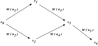
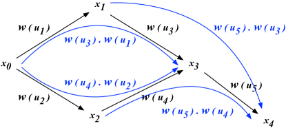
Figure 1: (left-to-right): Weighted quivers (a) $\Gamma$ and (b) $\operatorname{Path}_{2}(\Gamma)$.

3 A Feature Map using Weighted Quiver Homology

In this section, we define a homology theory for weighted quivers, with which a new “weighted quiver kernel” is defined. Throughout this section, we fix a commutative ring $k$. When necessary, we assume that $k$ is a field.

3.1 Homology of Small Categories

Let us first recall the definition of homology of small categories. The definition can be regarded as a variant of the homology of a simplicial complex. We first construct the nerve complex $N(C)$ from a small category $C$. The nerve complex has a structure analogous to simplicial complexes. Thus we may define its homology.

In order to understand the definition of homology of small categories, let us first recall the definition of simplicial complexes and their homology.

Definition 3.1.

Let $K$ be a simplicial complex with vertex set $V$. For each nonnegative integer $n$, the free Abelian group generated by the $n$-dimensional simplices of $K$ is denoted by $C_{n}(K;\mathbb{Z})$. More generally, for a commutative ring $k$, we may form a free $k$-module instead of a free Abelian group to obtain $C_{n}(K;k)$.

In order to make the collection $C_{*}(K;k)=\{C_{n}(K;k)\}_{n\geq 0}$ into a chain complex, we assume that the vertex set $V$ is totally ordered. When a simplex $\sigma$ has vertices $x_{0},\ldots,x_{n}$ with $x_{0}<\cdots<x_{n}$, we denote $\sigma=[x_{0},\ldots,x_{n}]$. Now the $n$-th boundary homomorphism $\partial_{n}:C_{n}(K;k)\to C_{n-1}(K;k)$ is defined by

$$\partial_{n}([x_{0},\ldots,x_{n}])=[x_{1},\ldots,x_{n}]+\sum_{i=1}^{n-1}(-1)^{i}[x_{0},\ldots,x_{i-1},x_{i+1},\ldots,x_{n}]+(-1)^{n}[x_{0},\ldots,x_{n-1}].$$ (1)

These maps make $C_{*}(K;k)$ into a chain complex, i.e. $\partial_{n}\circ\partial_{n+1}=0$ for all $n$.

The $n$-th homology group of $K$ with coefficients in $k$ is defined by

$$H_{n}(K;k)=\operatorname{Ker}(\partial_{n}:C_{n}(K;k)\to C_{n-1}(K;k))/\operatorname{Im}(\partial_{n+1}:C_{n+1}(K;k)\to C_{n}(K;k)).$$

When $Q$ is a simple quiver, any element of $N_{n}(Q)$ can be represented by a sequence of vertices $(v_{0},\ldots,v_{n})$, as we have observed in Remark 2.5. An obvious idea is to form free $k$-modules generated by the sets $N_{n}(Q)$ and define boundary homomorphisms by a formula similar to (1). Unfortunately, $(x_{i-1},x_{i+1})$ may not be an arrow in $Q$, even if both $(x_{i-1},x_{i})$ and $(x_{i},x_{i+1})$ are arrows in $Q$. The boundary homomorphism $\partial_{n}$ cannot be defined.

For a small category, however, we may always compose morphisms to get a new morphism. Thus we may define a chain complex. In order to simplify the description, we restrict ourselves to the case of acyclic categories.

Definition 3.2.

A small category $C$ is called acyclic if

1. for distinct objects $x,y$, either $C(x,y)$ or $C(y,x)$ is empty, and

2. for any object $x$, the only morphism from $x$ to $x$ is the identity.

Definition 3.3.

An $n$-chain $(u_{n},\ldots,u_{1})$ in $C$ is called nondegenerate if none of $u_{i}$’s is an identity morphism. For $n\geq 1$, the set of nondegenerate $n$-chains in $C$ is denoted by $\overline{N}_{n}(C)$. We also define $\overline{N}_{0}(C)=N_{0}(C)$.

The submodule of $C_{n}(C;k)$ generated by $\overline{N}_{n}(C)$ is denoted by $\overline{C}_{n}(C;k)$.

Example 3.4.

When a quiver $Q$ does not contain a loop or an oriented cycle, $F(Q)$ is an acyclic category.

Definition 3.5.

Let $C$ be a small acyclic category and $k$ a commutative ring. The collection $\overline{C}_{*}(C;k)=\{\overline{C}_{n}(C;k)\}_{n\geq 0}$ can be made into a chain complex by defining the boundary homomorphisms as follows. When $n=1$

$$\bar{\partial}_{1}(u)=t(u)-s(u).$$

For $n\geq 2$,

$$\bar{\partial}_{n}(u_{n},\ldots,u_{1})=(u_{n},\ldots,u_{2})+\sum_{i=1}^{n-1}(-1)^{i}(u_{n},\ldots,u_{i+1}\circ u_{i},\ldots,u_{1})+(-1)^{n}(u_{n-1},\ldots,u_{1}).$$

Note that $\bar{\partial}_{n}=0$ for $n\leq 0$ by definition.

The $n$-th homology of $C$ with coefficients in $k$ is defined by

$$H_{n}(C;k)=\operatorname{Ker}\bar{\partial}_{n}/\operatorname{Im}\bar{\partial}_{n+1}.$$

Remark 3.6.

The homology groups can be defined for arbitrary small categories. See Appendix A for details.

3.2 Homology of Weighted Quivers and Categories

Now suppose that our category $C$ is equipped with a weight function $w$ with values in a monoid $W$. We would like to put this information into the homology of $C$. This can be done when $W$ acts on a $k$-module $M$ from the left, meaning that, for $x\in W$ and $m\in M$, an element $xm\in M$ is given in such a way that

1. $x(m+m^{\prime})=xm+xm^{\prime}$ for $x\in W$ and $m,m^{\prime}\in M$,

2. $x(\alpha m)=\alpha xm$ for $x\in W$, $\alpha\in k$, and $m\in M$,

3. $x(x^{\prime}m)=(xx^{\prime})m$ for $x,x^{\prime}\in W$ and $m\in M$, and

4. $1m=m$, where $1$ is the unit of $W$.

In other words, $M$ is a representation of $W$.

With this information, we modify the definition of homology as follows.

Definition 3.7.

Let $C$ be a small acyclic category with a weight function $w:C_{1}\to W$ and $M$ a representation of $W$. For each nonnegative integer $n$, define a $k$-module

$$\overline{C}_{n}(C,w;M)=\overline{C}_{n}(C;k)\otimes M,$$

where the tensor product is taken over $k$. The boundary homomorphisms are given as follows. When $n=1$

$$\bar{\partial}^{M}_{1}(u\otimes m)=t(u)\otimes w(u)m-s(u)\otimes m.$$

For $n\geq 2$,

$$\bar{\partial}^{M}_{n}(u_{n},\ldots,u_{1})=(u_{n},\ldots,u_{2})\otimes w(u_{1})m+\sum_{i=1}^{n-1}(-1)^{i}(u_{n},\ldots,u_{i+1}\circ u_{i},\ldots,u_{1})\otimes m\\ +(-1)^{n}(u_{n-1},\ldots,u_{1})\otimes m,$$

It is elementary to verify that these maps define a chain complex $\overline{C}_{*}(C,w;M)$. The $n$-th homology of $C$ with coefficients in $M$ is defined by

$$H_{n}(C,w;M)=\operatorname{Ker}\bar{\partial}^{M}_{n}/\operatorname{Im}\bar{\partial}^{M}_{n+1}.$$

When $\Gamma=(Q,w)$ is a weighted quiver, we have a canonical extension to a weighted small category $(F(Q),\widetilde{w})$ by Lemma 2.11 and Example 2.13. We denote

$$H_{n}(\Gamma;M)=H_{n}(Q,w;M)=H_{n}(F(Q),\widetilde{w};M).$$

This is called the homology of $(Q,w)$ with coefficients in $M$.

This homology group can be regarded as a special case of a construction, known as the homology of a small category with coefficients in a functor. A precise meaning is recorded in Appendix A.

In general, it is not easy to compute the homology of a small category. Fortunately, for categories of the form $F(Q)$, a very small chain complex for computing the homology is known, which gives us the following description of $H_{*}(Q,w;M)$.

Theorem 3.8.

Let $\Gamma=(Q,w)$ be a finite acyclic weighted quiver with weights in a monoid $W$ and $M$ be a representation of $W$. Define a map

$$\varphi:\bigoplus_{u\in Q_{1}}k\{u\}\otimes M\buildrel\over{\longrightarrow}\bigoplus_{x\in Q_{0}}k\{x\}\otimes M$$

by

$$\varphi(u\otimes m)=t(u)\otimes m-s(u)\otimes\left(w(u)\cdot m\right).$$

Then $H_{n}(Q,w;M)=0$ for $n\geq 2$ and

$$H_{1}(Q,w:M)=\operatorname{Ker}\varphi.$$

We need to prepare the language of homological algebra to prove this theorem. A proof is given in Appendix A.2.

We conclude this section by making sample computations of homology of weighted networks.

Example 3.9.

Let $\Gamma=(Q,w)$ be a simple weighted quiver with three vertices $x_{1},x_{2},x_{3}$ shown in Figure 2, where $w_{1}=w(x_{1},x_{0})$, $w_{2}=w(x_{2},x_{1})$, and $w_{3}=w(x_{2},x_{0})$.

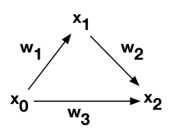
Figure 2: The weighted quiver $\Gamma$

There are two routes from $x_{0}$ to $x_{2}$ in this network; the direct route $x_{0}\to x_{2}$ costs $w_{3}$ while the route $x_{0}\to x_{1}\to x_{2}$ costs

$$w(x_{2},x_{1},x_{0})=w(x_{2},x_{1})w(x_{1},x_{0})=w_{2}w_{1}.$$

We would like to know the costs of these two routes are equal or not. Let us show that this problem can be solved by computing the first homology of the weighted category $(F(Q),w)$.

Suppose that $k$ is a field and that $W$ is a submonoid of $k^{\times}=k\setminus\{0\}$. Note that the monoid operation on $W$ is given by the multiplication of $k$. Then $W$ acts on $k$ by the multiplication. The module $k$ with this action is denoted by $k(w)$. Let us compute

$$H_{1}(\Gamma;k(w))=H_{1}(Q,w;k(w))=H_{1}(F(Q),\widetilde{w};k(w))$$

under these conditions.

By Theorem 3.8, it suffices to determine $\operatorname{Ker}\varphi$. The domain of the map $\varphi$ is a vector space with bases $Q_{1}$, which consists of three elements $(x_{1},x_{0})$, $(x_{2},x_{1})$, and $(x_{2},x_{0})$. The range of $\varphi$ has basis $Q_{0}=\{x_{0},x_{1},x_{2}\}$.

With these bases the map $\varphi$ is given by

$$\bar{\partial}_{1}((x_{1},x_{0})\otimes 1) =x_{1}\otimes w_{1}\cdot 1-x_{0}\otimes 1$$

$$=(-1)(x_{0}\otimes 1)+w_{1}(x_{1}\otimes 1)+0(x_{2}\otimes 1)$$

$$\bar{\partial}_{1}((x_{2},x_{1})\otimes 1) =x_{2}\otimes w_{2}\cdot 1-x_{1}\otimes 1$$

$$=0(x_{0}\otimes 1)+(-1)(x_{1}\otimes 1)+w_{2}(x_{2}\otimes 1)$$

$$\bar{\partial}_{1}((x_{2},x_{0})\otimes 1) =x_{2}\otimes w_{3}\cdot 1-x_{0}\otimes 1$$

$$=(-1)(x_{0}\otimes 1)+0(x_{1}\otimes 1)+w_{3}(x_{2}\otimes 1).$$

In other words, the map $\varphi$ is given by the following matrix

$$\begin{pmatrix}-1&0&-1\\ w_{1}&-1&0\\ 0&w_{2}&w_{3}\end{pmatrix}$$

and $\operatorname{Ker}\varphi$ can be identified with the solution to the linear equation

$$\begin{pmatrix}-1&0&-1\\ w_{1}&-1&0\\ 0&w_{2}&w_{3}\end{pmatrix}\begin{pmatrix}a\\ b\\ c\end{pmatrix}=\begin{pmatrix}0\\ 0\\ 0\end{pmatrix}.$$

The determinant of this matrix is

$$\det\begin{pmatrix}-1&0&-1\\ w_{1}&-1&0\\ 0&w_{2}&w_{3}\end{pmatrix}=w_{3}-w_{1}w_{2}.$$

Thus

$$\dim\operatorname{Ker}\varphi=\begin{cases}1,&w_{2}w_{1}=w_{3}\\ 0,&w_{2}w_{1}\neq w_{3}.\end{cases}$$

When $w_{3}=w_{1}w_{2}$, a basis for $\operatorname{Ker}\varphi$ can be taken to be the vector $\begin{pmatrix}1\\ w_{1}\\ -1\end{pmatrix}$.

Thus the first homology is given by

$$H_{1}(\Gamma;k(w))=\operatorname{Ker}\varphi\cong\begin{cases}k\left\langle\begin{pmatrix}1\\ w_{1}\\ -1\end{pmatrix}\right\rangle,&w_{2}w_{1}=w_{3}\\ 0,&w_{2}w_{1}\neq w_{3},\end{cases}$$

which means that we can distinguish two cases by looking at the first homology.

Example 3.10.

Consider the weighted quiver $\Sigma=(S,w)$ in Figure 3.

$$\begin{diagram}$$

Figure 3: The square quiver $\Sigma$.

The map $\varphi$ is given by

$$\varphi((x_{2},x_{1})\otimes 1) =x_{2}\otimes w_{1}\cdot 1-x_{1}\otimes 1$$

$$=(-1)(x_{1}\otimes 1)+w_{1}(x_{2}\otimes 1)+0(x_{3}\otimes 1)+0(x_{4}\otimes 1)$$

$$\bar{\partial}_{1}((x_{4},x_{2})\otimes 1) =x_{4}\otimes w_{2}\cdot 1-x_{2}\otimes 1$$

$$=0(x_{1}\otimes 1)+(-1)(x_{2}\otimes 1)+0(x_{3}\otimes 1)+w_{2}(x_{4}\otimes 1)$$

$$\bar{\partial}_{1}((x_{3},x_{1})\otimes 1) =x_{3}\otimes w_{3}\cdot 1-x_{1}\otimes 1$$

$$=(-1)(x_{1}\otimes 1)+0(x_{2}\otimes 1)+w_{3}(x_{3}\otimes 1)+0(x_{4}\otimes 1)$$

$$\bar{\partial}_{1}((x_{4},x_{3})\otimes 1) =x_{4}\otimes w_{4}\cdot 1-x_{3}\otimes 1$$

$$=0(x_{1}\otimes 1)+0(x_{2}\otimes 1)+(-1)(x_{3}\otimes 1)+w_{4}(x_{4}\otimes 1).$$

The matrix representation is

$$D=\begin{pmatrix}-1&0&-1&0\\ w_{1}&-1&0&0\\ 0&0&w_{3}&-1\\ 0&w_{2}&0&w_{4}\end{pmatrix}.$$

This matrix can be made into the following matrix by row transformations.

$$\widetilde{D}=\begin{pmatrix}-1&0&-1&0\\ 0&-1&-w_{1}&0\\ 0&0&w_{3}&-1\\ 0&0&w_{4}w_{3}-w_{2}w_{1}&0\end{pmatrix}.$$

The rank of this matrix is

$$\operatorname{rank}D=\operatorname{rank}\widetilde{D}=\begin{cases}3,&\text{ if }w_{4}w_{3}=w_{2}w_{1},\\ 4,&\text{ if }w_{4}w_{3}\neq w_{2}w_{1}.\end{cases}$$

Thus we obtain

$$\dim H_{1}(\Sigma;k(w))=\dim\operatorname{Ker}\bar{\partial}_{1}=4-\operatorname{rank}D=\begin{cases}1,&\text{ if }w_{4}w_{3}=w_{2}w_{1},\\ 0,&\text{ if }w_{4}w_{3}\neq w_{2}w_{1}.\end{cases}$$

Again we may tell if $w_{4}w_{3}=w_{2}w_{1}$ or not by computing the first homology.

3.3 A Weighted Quiver Kernel by Homology

After having introduced the necessary terminology and developed a weighted quiver homology, we are now ready to describe our method for constructing feature vectors.

Before we describe our algorithm, we explain how one constructs an acyclic quiver (or directed acyclic graph (DAG)) from a simple quiver (or directed graph). In order to break cycles and leave a quiver “acyclic”, one must identify and remove a minimum set of arrows. In graph theory, this is a well-known NP-hard problem, referred to as the minimum feedback arc set problem. Due to the NP-hard nature of this problem, we resort to a randomized approximation algorithm proposed by Berger and Shor [2].

Input: Simple weighted quiver $\Gamma=(Q,w)$

Output: A feedback arc set $F$ for $\Gamma$

/* Initialization of Feedback arc set with empty set */

1 $F\leftarrow\emptyset$

2

/* Process vertices in a fixed permuted order */

3 for  $v\in\Pi(Q_{0})$  do

       /* if there are more incoming arrows than outgoing ones... */

4       if  $\delta_{in}(v)>\delta_{out}(v)$  then

5             $E_{1}:=\{e\mid e\in Q_{1},s(e)=v\}$

6             $F\leftarrow F\cup E_{1}$

7            

8      else

9             $E_{2}:=\{e\mid e\in Q_{1},t(e)=v\}$

10             $F\leftarrow F\cup E_{2}$

11            

      /* Discard edges $E_{1}\cup E_{2}$ from $Q_{1}$ */

12       $Q_{1}\leftarrow Q_{1}\setminus(E_{1}\cup E_{2})$

/* Set of feedback arcs dropped from $\Gamma$ */

13 return $F$

Algorithm 1 Berger and Shor Algorithm to compute Feedback Arc Set.

For the sake of completeness, Algorithm 1 describes the Berger and Shor algorithm in detail. This algorithm begins by choosing a random permutation $\Pi(Q_{0})$ of the vertices of the incoming quiver $\Gamma$. The vertices are processed in the order given by the permutation (Line $2$). If a given vertex $v$ has more incoming arrows than outgoing ones, then $E_{1}$ contains the outgoing nodes and this is added to our feedback set $F$ (Lines $3$–$5$). The opposite case is handled on Lines $7$–$8$. The edges in $E_{1}\cup E_{2}$ are removed from $Q_{1}$ and the remaining arrows make $\Gamma$ acyclic. The set $F$ contains the feedback arcs/arrows that are dropped.

The intuition behind this approach is that we choose to keep either the incoming or outgoing arrows at any given time which ensures that the resulting quiver is acyclic. Additionally, we choose to keep the set of incoming or outgoing arrows with larger cardinality, thus resulting in a larger acyclic quiver. This randomized algorithm runs in $O(M+N)$ (where $M$ and $N$ denote the number of arrows and vertices in the quiver) and produces an acyclic quiver containing at least $1/2+\Omega(1/\sqrt{\delta_{max}})|Q_{0}|$ arrows, where $\delta_{max}$ is the maximum degree of any vertex in $Q_{0}$.

Input: Simple weighted quiver $\Gamma=(Q,w)$, Number of iterations $H$, Total number of nodes $N$ and arrows $M$ in $Q$

Output: Feature matrix $X\in\mathds{Z}^{N\times H}$ representing $\Gamma$

/* Initialization */

1 $X\leftarrow$ Empty $N\times H$ matrix

2 $i\leftarrow 0$

3

4for  $v\in Q_{0}$  do

5       $i\leftarrow i+1$

6      

7      for  $k\in\{1\dots H\}$  do

8             $N_{k}(v)\leftarrow$ Set of vertices in $Q$ within $k$-hops from $v$

             /* Makes use of Algorithm 1 to build DAG */

9             $Q^{\prime}_{k}\leftarrow$ Sub-quiver DAG induced by vertices in $N_{k}(v)$

10             $(n,m)\leftarrow$ (# of nodes, # of edges) in $Q^{\prime}_{k}$

             /* Build the boundary matrix $D$ for subquiver $Q^{\prime}_{k}$ */

11             $D\leftarrow$ Empty $n\times m$ matrix

12             foreach  arrow $u\buildrel w^{\prime}\over{\longrightarrow}v$ in $Q^{\prime}_{k}$  do

13                   $D[u,i]\leftarrow-1$

14                   $D[v,i]\leftarrow w^{\prime}$

15                  

16            $rank(D)\leftarrow$ Compute rank of matrix $D$

             /* Get $dimH_{1}(Q^{\prime}_{k},w^{\prime};k(w^{\prime})$ */

17             $X[i,k]\leftarrow m-rank(D)$

18      

19return $X$

Algorithm 2 Computes feature vectors based on weighted quiver homology.

Algorithm 2 describes in detail all the steps required for feature computation. A high-level description of our algorithm consists of the following operations.

For every vertex $v$ in the underlying quiver’s vertex set $Q_{0}$ (line $3$), we iterate $H$ times, each time computing a progressively larger acyclic sub-quiver (in the form of a directed acyclic graph (DAG)) and its weighted quiver homology (lines $6$–$14$). Note that the variable $k$ ranges from $1$ to $H$, and in each iteration for a given value of $k$, we compute the set of vertices $N_{k}(v)$ that are $k$-hops away from $v$, i.e., the set of vertices with a directed path of length at most $k$ from $v$. Finally, the dimensions of the first homology for each $k$ are concatenated to form a vector of size $H$ (line $14$). For a given simple weighted quiver $\Gamma=(Q,w)$ with $N$ nodes and $M$ arrows, our procedure results in $N$ feature vectors, each of size $H$.

Time complexity

The dominant costs in our computation are incurred by the matrix rank computation and computing the $k$-hop neighborhood.

To begin with, we analyze the rank computation cost. In the worst case, the dimension of matrix $D$ representing a sub-quiver is $N\times M$, when the sub-quiver is the same as the quiver $Q$. According to Golub and Van Loan [7] the best known rank computation algorithms that internally involve singular value decomposition (SVD) for a $N\times M$ matrix has a time complexity of $O(NM^{2})$.

Next, we study the cost of computing the $k$-hop neighborhood. Let $N^{(k)}_{\max}$ and $M^{(k)}_{\max}$ denote the maximum number of vertices and edges, respectively, in a subquiver induced by a $k$-hop neighborhood around a vertex. Then, steps in lines $6$–$7$ have a time-complexity of $O(N^{(k)}_{\max}+M^{(k)}_{\max})$.

Then, lines $6$–$14$, have a total complexity of $O(N^{(k)}_{\max}+M^{(k)}_{\max}+NM^{2})$. As this is repeated for each vertex (i.e., $N$ of them) and for $H$ times, we get an overall time complexity of $O(NH(N^{(k)}_{\max}+M^{(k)}_{\max}+NM^{2}))$.

4 Applications

In this section, we illustrate the practical applicability of our weighted quiver homology and its corresponding feature vectors to two well-known tasks on real-world multi-graphs in machine learning and other graph / network analysis research literature. Namely, we focus on: (i) Creating node embeddings for weighted directed graphs and (ii) detecting communities in weighted directed graphs.

4.1 Node Embeddings of Weighted Directed Graphs

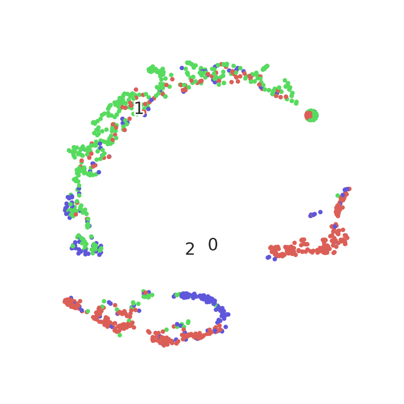
(a) $H=4$

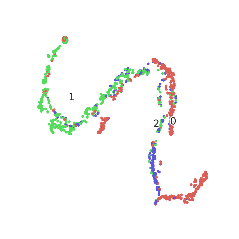
(b) $H=5$

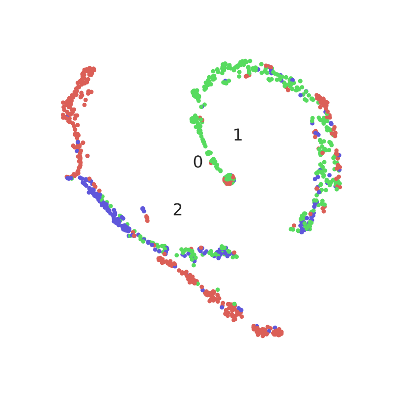
(c) $H=6$

Figure 4: t-SNE plots of the node embeddings as we vary $H$ in Algorithm 2. With increasing $H$, we notice a better separation of nodes pertaining to different labels / categories. Higher the separation achieved, better the quality of the node embedding.

Given the ubiquitous prevalence of graphs, their analysis in areas like machine learning (ML) plays a fundamental role. In order to apply existing ML methods to graphs (e.g., to predict new interactions or discover latent relations between objects represented as nodes / vertices), one learns a representation of the graph that is amenable to be used in ML algorithms.

However, graphs are inherently unordered, irregular, and combinatorial in nature made up of nodes / vertices and edges / links between nodes, while most ML methods (e.g. neural networks) favor continuous vector representations. To get around the difficulties in using discrete graph representations in ML, graph embedding methods learn a continuous vector space for the graph, assigning each node (and/or edge) in the graph to a specific position in a vector space. We refer the reader to a survey on node embeddings [3] for more details.

Task:

More formally, given a weighted directed graph $G=(V,E,W)$, where $V$ and $E$ denote the set of nodes and directed edges (arrows) connecting them. $W$ is the set of edge weights corresponding to each directed edge $e=(u,v)\in E$. The graph $G$ can be represented by a weighted adjacency matrix $A\in\mathds{R}^{|V|\times|V|}$, where the $u,v$-th element in $A$, i.e., $A_{u,v}$ has a value which corresponds to the edge weight in $W$ of the directed edge $(u,v)$. In general, node embedding methods try to minimize an objective

$$\min_{Y}L(f(A),g(Y))$$

where $Y\in\mathds{R}^{|V|\times d}$, for $d\ll|V|$ is a $d$-dimensional node embedding matrix; $f:\mathds{R}^{|V|\times|V|}\buildrel\over{\longrightarrow}\mathds{R}^{|V|\times|V|}$ is a transformation of the weighted adjacency matrix; $g:\mathds{R}^{|V|\times d}\buildrel\over{\longrightarrow}\mathds{R}^{|V|\times|V|}$ is a pairwise edge function; and $L:\mathds{R}^{|V|\times|V|}\buildrel\over{\longrightarrow}\mathds{R}^{|V|\times|V|}$ is a loss function.

Dataset:

For our empirical evaluation, we used the popular Cora dataset [13]. The Cora dataset is a research citation network (directed) comprising of $2708$ scientific publications classified into one of seven categories. The citation network consists of $5429$ links. Each publication (vertex) in the dataset is described by a $0/1$-valued word vector indicating the absence/presence of the corresponding word from the dictionary. The dictionary consists of $1433$ unique words. Thus, each vertex has a corresponding binary vector of length $1433$.

Experimental Setup:

For our experiment, we only focused on a subset of the categories, i.e., three categories, namely Genetic_Algorithms (Label $0$), Probabilistic_Methods (Label $1$), and Reinforcement_Learning (Label $2$). We computed an edge weight for each edge as the Jaccard distance between the vectors associated with the start and terminal vertices of the edge.

Results:

In Figure 4, we notice that as we increase the number of iterations $H$ in our method, we get a larger dimensional feature vector which starts to achieve better separation of topics / labels among the nodes in the citation network. Therefore, nodes that represent a given topic cluster together and also move away from topics that are different. We see this separation improve as we vary $H$ from $4$ to $6$. In order to visualize these $H$-dimensional vectors representing the nodes in the Cora graph, we used $t$-Distributed Stochastic Neighbor Embedding (t-SNE) [15], which is a technique for dimensionality reduction that is particularly well suited for the visualization of high-dimensional datasets.

4.2 Community Detection in Weighted Graphs

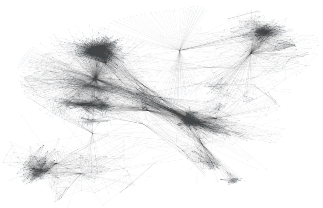
(a) Original graph

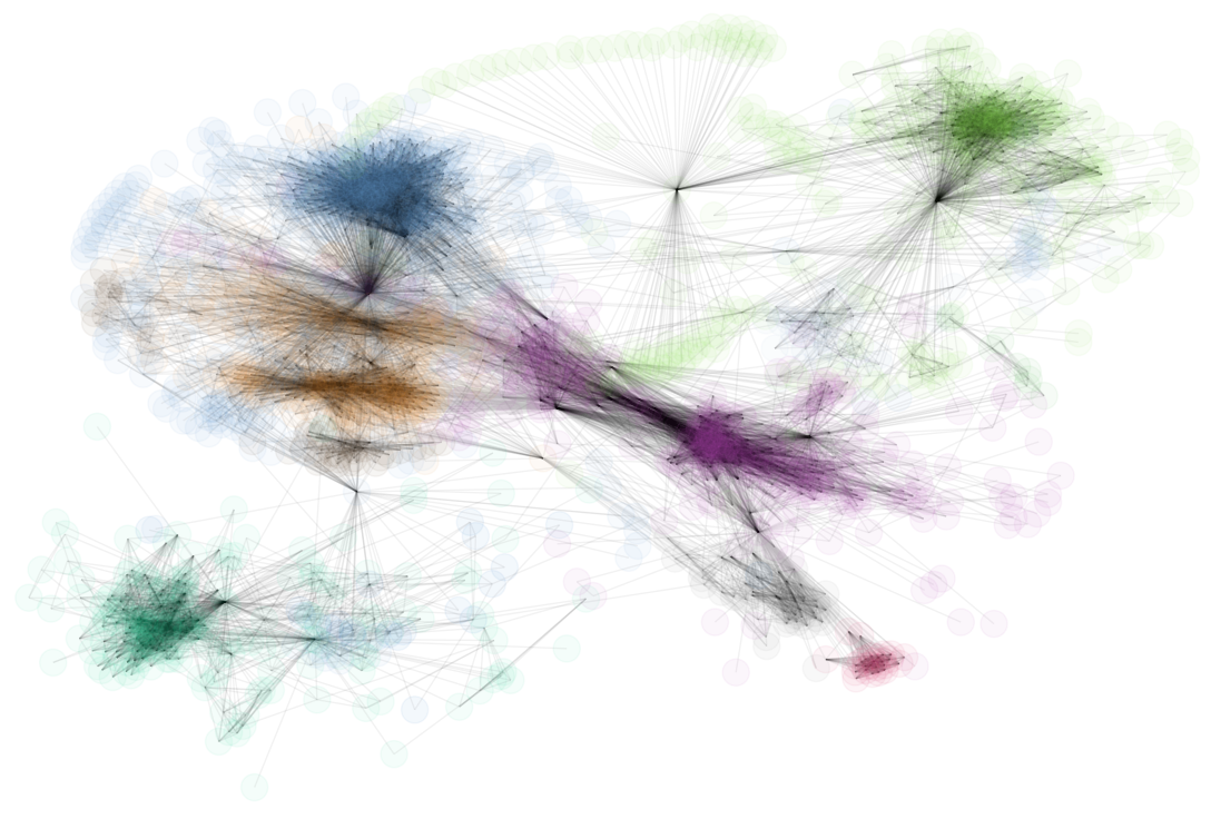
(b) Communities marked in original graph

Figure 5: Seven distinct communities (marked with different colored nodes) detected using weighted quiver homology features in Facebook graph with $2094$ nodes and $20$K edges.

Complex systems can be represented in terms of graphs, where the elements composing the complex system are described as nodes / vertices and their interactions as edges / links. At a global level, the nature of these interactions is far from trivial and very complex in nature. At a mesoscopic (intermediate) scale, it is possible to identify a group of nodes that are densely connected among themselves, but sparsely connected to the rest of the graph. Such heavily interconnected group of vertices are often characterized as communities and occur in a wide variety of networked systems. For example, such communities can be considered as independent portions of a graph, playing a similar role, like the tissues or the organs in the human body. Community detection finds applications in a wide and diverse set of areas such as biology, sociology, and computer science, to name a few, where systems are often represented as graphs. This problem is extremely hard and has not yet been solved satisfactorily, despite the huge effort of a large interdisciplinary community of scientists working on it over the past few years. This task gets even harder when having to identify such communities in weighted directed graphs. We refer the reader to a survey on community detection [5] for more details.

Task:

Given a graph $G=(V,E)$, we denote the degree of a node $u$ by $\delta_{u}$. If we consider a subset of nodes $V^{\prime}\subseteq V$ that are densely connected and represent a community, to which node $u$ belongs. We denote the sum of degrees of the nodes present in $V^{\prime}$ by $\delta_{u}(V)$. Then, this total degree can be split into two contributions

$$\delta_{u}(V)=\delta_{u}^{in}(V^{\prime})+\delta_{u}^{out}(V^{\prime})$$

where $\delta_{u}^{in}(V^{\prime})$ is the number of edges connecting $u$ to other nodes in $V^{\prime}$ and $\delta_{u}^{out}(V^{\prime})$ is the number of edges connecting $u$ to $V\setminus V^{\prime}$ (i.e., rest of the nodes outside $V^{\prime}$). The subset $V^{\prime}$ is a termed a community in the strong sense, if

$$\delta_{u}^{in}(V^{\prime})>\delta_{u}^{out}(V^{\prime})\text{, \hskip 20.00003pt}\forall u\in V^{\prime}$$

Dataset:

We downloaded the Facebook graph dataset from SNAP [12]. This dataset consists of circles (or friends lists) from Facebook. Facebook data was collected from survey participants using this Facebook application. We used a smaller subset of the large graph, by taking into account $2094$ vertices and $20$K edges connecting them.

Experimental Setup:

As this was an undirected graph dataset, we assigned an orientation to each edge $(u,v)$, by setting $u\buildrel\over{\longrightarrow}v$, if $u<v$, and $u\buildrel\over{\longleftarrow}v$, if $u>v$. Accordingly, an edge weight was also assigned as $|u-v|$. $H$ was fixed at $3$, in our experiments. We first computed a node embedding as was done in Section 4.1, ran a DBSCAN density-based clustering, and mapped the clusters back to the original nodes in the graph.

Results:

We detected $7$ different communities that are each uniquely colored and depicted in Figure 5(b). It can be visually observed that our method does a fairly good job of detecting communities in the strong sense in the Facebook graph.

Appendix A Mathematics for Homology of Small Categories

In this appendix, we collect precise mathematical definitions and statements for those who have enough mathematical backgroud. Here we assume that the reader is familiar with basic category theory and algebraic topology, including simplicial homotopy theory.

A.1 Homology of Small Categories with Coefficients in Functors

Recall that we have introduced the set $N_{n}(Q)$ of $n$-chains in a quiver $Q$. By regarding a small category $C$ as a quiver, we have a collection $\{N_{n}(C)\}_{n\geq 0}$ of sets. When $C$ is a category, this collection has a structure of simplicial set.

Lemma A.1.

For a small category $C$, the collection $N(C)=\{N_{n}(C)\}_{n\geq 0}$ can be made into a simplicial set by the following operators. The face operators $d_{i}:N_{n}(C)\rightarrow N_{n-1}(C)$ are given as follows. When $n=1$, $d_{0}(u)=t(u)$ and $d_{1}(u)=s(u)$. When $n\geq 2$,

$$(u_{n},\ldots,u_{1}) =x_{0}\buildrel u_{1}\over{\longrightarrow}\dots\buildrel u_{i}\over{\longrightarrow}x_{i}\buildrel u_{i+1}\over{\longrightarrow}x_{i+1}\dots\buildrel u_{n}\over{\longrightarrow}x_{n}$$

$$\xmapsto{d_{i}}\left\{\begin{aligned} &x_{1}\buildrel u_{2}\over{\longrightarrow}x_{2}\dots\buildrel u_{n}\over{\longrightarrow}x_{n},&&\text{if}\ i=0\\ &x_{0}\buildrel u_{1}\over{\longrightarrow}\dots\buildrel\over{\longrightarrow}x_{i}\buildrel u_{i}\circ u_{i+1}\over{\longrightarrow}x_{i+2}\buildrel\over{\longrightarrow}\dots\buildrel u_{n}\over{\longrightarrow}x_{n},&&\text{if}\ 0<i<n\\ &x_{0}\buildrel u_{1}\over{\longrightarrow}\dots\buildrel u_{n-1}\over{\longrightarrow}x_{n-1},&&\text{if}\ i=n\end{aligned}\right.$$

The degeneracy operators $s_{i}:N_{n}(C)\to N_{n+1}(C)$ are defined by

$$s_{i}(u_{n},\ldots,u_{1})=(u_{n},\ldots,u_{i+1},1_{x_{i}},u_{i},\ldots,u_{1}).$$

This simplicial set is called the nerve of $C$.

There is a standard way to generate a chain complex from a simplicial set.

Definition A.2.

Let $k$ be a commutative ring. For a simplicial set $X$, the free $k$-module generated by $X_{n}$ is denoted by $C_{n}(X;k)$. Define

$$\partial_{n}:C_{n}(X;k)\buildrel\over{\longrightarrow}C_{n-1}(X;k)$$

by

$$\partial_{n}=\sum_{i=0}^{n}(-1)^{i}d_{i}.$$

The collection $C(X;k)=\{C_{n}(X;k),\partial_{n}\}$ forms a chain complex over $k$. The homology of this chain complex is denoted by

$$H_{n}(X;k)=H_{n}(C(X;k))=\operatorname{Ker}\partial_{n}/\operatorname{Im}\partial_{n+1}$$

and is called the homology group of $X$ with coefficients in $k$.

When $X=N(C)$ for a small category $C$, the homology of $N(C)$ with coefficients in $k$ is denoted by $H_{n}(C;k)$.

When $C$ is equipped with a functor $G:C\to{k}\text{-}\mathbf{Mod}$, we may modify the definition of the nerve and homology as follows.

Definition A.3.

Let $G:C\to{k}\text{-}\mathbf{Mod}$ be a functor on a small category $C$. Define

$$B_{n}(C;G)=\bigoplus_{x\in C_{0}}k\langle s^{-1}(x)\rangle\otimes G(x),$$

where $s:N_{n}(C)\to C_{0}$ is the map defined in Definition 2.1.

This collection of $k$-modules $B(C;G)=\{B_{n}(C;G)\}_{n}$ can be made into a simplicial $k$-module as follows. When $n=1$, the face operators are given by

$$d_{0}(u\otimes m) =t(u)\otimes G(u)(m)$$

$$d_{1}(u) =s(u)\otimes m.$$

When $n\geq 2$, the face operators are given by

$$d_{i}((u_{n},\ldots,u_{1})\otimes m)=\left\{\begin{aligned} &(u_{n},\ldots,u_{2})\otimes G(u_{1})(m),&&\text{if}\ i=0\\ &(u_{n},\ldots,u_{i+1}\circ u_{i},\ldots,u_{1})\otimes m,&&\text{if}\ 0<i<n\\ &(u_{n-1},\ldots,u_{1})\otimes m,&&\text{if}\ i=n\end{aligned}\right.$$

The degeneracy operators $s_{i}:B_{n}(C;G)\to B_{n+1}(C;G)$ are defined by

$$s_{i}((u_{n},\ldots,u_{1})\otimes m)=(u_{n},\ldots,u_{i+1},1_{x_{i}},u_{i},\ldots,u_{1})\otimes m.$$

The face operators can be assembled in the usual way to define a boundary operator

$$\partial_{n}=\sum_{i=0}^{n}(-1)^{i}d_{i}:B_{n}(C;G)\buildrel\over{\longrightarrow}B_{n-1}(C;G).$$

The homology of this chain complex is denoted by $H_{n}(C;G)$ and is called the homology of $C$ with coefficients in $G$.

Example A.4.

Let $w:C\to W$ be a weight function and $M$ a representation of $W$. When $W$ is regarded as a category with a single object $*$, the left action of $W$ on $M$ can be regarded as a covariant functor $\mu_{M}:W\to M$, which assigns $M$ to the unique object $*$ in $W$. Then the composition

$$F_{w}=\mu_{M}\circ w:C\buildrel\over{\longrightarrow}{k}\text{-}\mathbf{Mod}$$

is a functor given by $F_{w}(x)=M$ on objects and

$$F_{w}(u)(m)=w(u)\cdot m$$

for $u\in C_{1}$ and $m\in M$.

The homology of $C$ with coefficients in $F_{w}$ is essentially the homology defined in Definition 3.7.

A.2 Homology of Small Categories as a Derived Functor

The aim of this section is to prove Theorem 3.8. We first need a description of the homology of small category as a derived functor. In the rest of this section, we free use the language of homological algebra. We also use the following notation which simplifies descriptions of constructions related to small categories and functors.

Definition A.5.

Let $C$ be a small category. The $k$-linear category generated by $C$ is denoted by $kC$ so that $(kC)_{1}$ is the free $k$-module generated by $C_{1}$. The free $k$-module generated by $C_{0}$ is denoted by $kC_{0}$. We regard it as a coalgebra over $k$ under the diagonal on $C_{0}$. We regard $(kC)_{1}$ as a right $kC_{0}$-comodule via the source map $s$ and a left $kC_{0}$-comodule via the target map $t$.

For a left $kC_{0}$-comodule $M$, define $kC\Box_{C_{0}}M$ by the following equalizer diagram

where $\delta_{M}$ is the comodule structure map of $M$.

A left $C$-module is a left $kC_{0}$-comdule $M$ equipped with a map

$$\mu_{M}:kC\Box_{C_{0}}M\buildrel\over{\longrightarrow}M$$

satisfying the associativity and unit conditions. Right $C$-modules are defined in a similar way by switching $kC$ and $M$. The categories of left and right $C$-modules are denoted by ${C}\text{-}\mathbf{Mod}$ and $\mathbf{Mod}\text{-}{C}$, respectively.

Example A.6.

Let $G:C\to{k}\text{-}\mathbf{Mod}$ be a functor. Define a $k$-module $\Gamma(G)$ by

$$\Gamma(G)=\bigoplus_{x\in C_{0}}G(x).$$

We regard $\Gamma(G)$ as a left $C_{0}$-comodule via

$$\delta_{G}(a)=x\otimes a$$

if $a\in G(x)$. Then

$$kC\Box_{C_{0}}\Gamma(G)=\bigoplus_{u\in C_{1}}k\{u\}\otimes G(s(u)).$$

The induced map $G(u):G(s(u))\to G(t(u))$ induces a map

$$k\{u\}\otimes G(s(u))\buildrel\over{\longrightarrow}G(t(u)),$$

which defines a structure of left $kC$-module on $\Gamma(G)$.

Similarly, a contravariant functor $G:C^{\mathrm{op}}\to{k}\text{-}\mathbf{Mod}$ gives rise to a right $kC$-module $\Gamma(G)$.

It is well-known that categories ${C}\text{-}\mathbf{Mod}$ and $\mathbf{Mod}\text{-}{C}$ are Abelian categories with enough projectives. Thus we may define derived functors. We are interested in the derived functor of the following bifunctor.

Definition A.7.

Let $C$ be a small category. For a right $C$-module $N$ and a left $C$-module $M$, define a $k$-module $N\otimes_{C}M$ by the following coequalizer diagram

where $\mu_{N}$ and $\mu_{M}$ are module structure maps for $N$ and $M$, respectively.

Let $N=kC_{0}$, regarded as a right $C$-module via the target map $t:C_{1}\to C_{0}$. Then, for a functor $G:C\to{k}\text{-}\mathbf{Mod}$, we have the following isomorphism

$$B_{n}(C;G)\cong kC_{0}\otimes_{C}\underbrace{kC\Box_{C_{0}}\cdots\Box{C_{0}}kC}_{n+1}\otimes_{C}\Gamma(G),$$

which can be assembled into an isomorphism of chain complexes. Since the collection

$$\left\{\underbrace{kC\Box_{C_{0}}\cdots\Box{C_{0}}kC}_{n+1}\otimes_{C}\Gamma(G)\right\}_{n\geq 0}$$

is a projective resolution of $\Gamma(G)$ in ${C}\text{-}\mathbf{Mod}$, the general theory of derived functors implies the following description of homology of small categories.

Proposition A.8.

Let $G:C\to{k}\text{-}\mathbf{Mod}$ be a functor and

$$\cdots\buildrel\over{\longrightarrow}P_{n}\buildrel d_{n}\over{\longrightarrow}P_{n-1}\buildrel\over{\longrightarrow}\cdots\buildrel\over{\longrightarrow}P_{1}\buildrel d_{1}\over{\longrightarrow}P_{0}\buildrel\varepsilon\over{\longrightarrow}\Gamma(G)\buildrel\over{\longrightarrow}0$$

be a projective resolution of $\Gamma(G)$ in ${C}\text{-}\mathbf{Mod}$. Then we have a natural isomorphism

$$H_{n}(kC_{0}\otimes_{C}P_{*})\cong H_{n}(C;G)$$

for all $n\geq 0$.

When $C=F(Q)$ for a finite acyclic quiver $Q$, a very small projective resolution of left $C$-modules is known. The following description can be found in a lecture note by Crawley-Boevey [4].

Proposition A.9.

Let $Q$ be a finite acyclic quiver and $G:F(Q)\to{k}\text{-}\mathbf{Mod}$ be a functor. Then the following sequence is exact

$$0\buildrel\over{\longrightarrow}kF(Q)\Box_{Q_{0}}kQ_{1}\Box_{Q_{0}}\Gamma(G)\buildrel f\over{\longrightarrow}kF(Q)\Box_{Q_{0}}\Gamma(G)\buildrel g\over{\longrightarrow}\Gamma(G)\buildrel\over{\longrightarrow}0,$$ (2)

where $kQ_{1}$ is regarded as a right $kQ_{0}$-comodule via the source map and a left $kQ_{0}$-comodule via the target map. The maps $f$ and $g$ are defined by

$$g(a\otimes m) =G(a)(m),$$

$$f(a\otimes u\otimes m) =a\otimes G(u)(m)-au\otimes m.$$

The above sequence is called the standard resolution or the minimal resolution of $G$ over the free category $F(Q)$.

Theorem 3.8 is now a corollary to Proposition A.9.

Proof of Theorem 3.8.

Since (2) is a projective resolution, $H_{*}(F(Q);G)$ can be computed by using this resolution for any functor $G:F(Q)\to{k}\text{-}\mathbf{Mod}$. In the case of Theorem 3.8, the functor is given by

$$G(x)=M$$

for any $x\in Q_{0}$. Thus

$$\Gamma(G)=\bigoplus_{x\in Q_{0}}k\{x\}\otimes M.$$

For a left $kQ_{0}$-comodule $N$, we have a natural isomorphism

$$kQ_{0}\otimes_{F(Q)}(kF(Q)\Box_{Q_{0}}N)\cong N$$

induced by the target map $t:F(Q)\to Q_{0}$. In particular, $H_{*}(Q,w;M)$ is the homology of the complex

$$\cdots\buildrel\over{\longrightarrow}0\buildrel\over{\longrightarrow}kQ_{1}\Box_{Q_{0}}\Gamma(G)\buildrel\bar{f}\over{\longrightarrow}\bigoplus_{x\in Q_{0}}k\{x\}\otimes M$$

and we have $H_{n}(Q,w;M)=0$ for $n\geq 2$. And the induced map $\bar{f}$ is given by

$$\bar{f}(u\otimes m)=t(u)\otimes(w(u)\cdot m)-s(u)\otimes m.$$

This completes the proof of Theorem 3.8. ∎

References

- [1] L. Babai and L. Kučera. Canonical labelling of graphs in linear average time. In 20th Annual Symposium on Foundations of Computer Science, pages 39–46, San Juan, Puerto Rico, 29–31 Oct. 1979. IEEE.
- [2] B. Berger and P. W. Shor. Approximation algorithms for the maximum acyclic subgraph problem. pages 236–243, San Francisco, CA, USA, Jan. 1990. SIAM.
- [3] H. Chen, B. Perozzi, R. Al-Rfou, and S. Skiena. A Tutorial on Network Embeddings.
- [4] W. Crawley-Boevey. Lectures on representations of quivers.
- [5] S. Fortunato. Community detection in graphs. Phys. Rep., 486(3-5):75–174, 2010.
- [6] T. Gärtner, P. Flach, and S. Wrobel. On graph kernels: Hardness results and efficient alternatives. In Proceedings of the 16th Annual Conference on Computational Learning Theory and 7th Kernel Workshop, pages 129–143. Springer-Verlag, Aug. 2003.
- [7] G. H. Golub and C. F. Van Loan. Matrix computations. Johns Hopkins Studies in the Mathematical Sciences. Johns Hopkins University Press, Baltimore, MD, fourth edition, 2013.
- [8] A. A. Husainov. Homological dimension theory of small categories. volume 110, pages 2273–2321. 2002. Algebra, 17.
- [9] R. Kanda. Construction of Grothendieck categories with enough compressible objects using colored quivers. J. Pure Appl. Algebra, 224(1):53–65, 2020.
- [10] H. Kashima, K. Tsuda, and A. Inokuchi. Marginalized kernels between labeled graphs. In T. Fawcett and N. Mishra, editors, Machine Learning, Proceedings of the Twentieth International Conference (ICML 2003), August 21-24, 2003, Washington, DC, USA, pages 321–328. AAAI Press, 2003.
- [11] N. M. Kriege, F. D. Johansson, and C. Morris. A survey on graph kernels. Applied Network Science, 5(1):6, 2020.
- [12] J. J. McAuley and J. Leskovec. Learning to discover social circles in ego networks. In P. L. Bartlett, F. C. N. Pereira, C. J. C. Burges, L. Bottou, and K. Q. Weinberger, editors, Advances in Neural Information Processing Systems 25: 26th Annual Conference on Neural Information Processing Systems 2012. Proceedings of a meeting held December 3-6, 2012, Lake Tahoe, Nevada, United States, pages 548–556, 2012.
- [13] P. Sen, G. M. Namata, M. Bilgic, L. Getoor, B. Gallagher, and T. Eliassi-Rad. Collective classification in network data. AI Magazine, 29(3):93–106, 2008.
- [14] N. Shervashidze, P. Schweitzer, E. J. van Leeuwen, K. Mehlhorn, and K. M. Borgwardt. Weisfeiler-Lehman graph kernels. J. Mach. Learn. Res., 12:2539–2561, 2011.
- [15] L. van der Maaten and G. Hinton. Visualizing data using t-sne. Journal of Machine Learning Research, 9:2579–2605, Nov. 2008.