Investigation of high-pressure turbulent jets using direct numerical simulation

Abstract

Direct numerical simulations of free round jets at a Reynolds number ($Re_{D}$) of $5000$, based on jet diameter ($D$) and jet-exit bulk velocity ($U_{e}$), are performed to study jet turbulence characteristics at supercritical pressures. The jet consists of Nitrogen ($\mathrm{N_{2}}$) that is injected into $\mathrm{N_{2}}$ at same temperature. To understand turbulent mixing, a passive scalar is transported with the flow at unity Schmidt number. Two sets of inflow conditions that model jets issuing from either a smooth contraction nozzle (laminar inflow) or a long pipe nozzle (turbulent inflow) are considered. By changing one parameter at a time, the simulations examine the jet-flow sensitivity to the thermodynamic condition (characterized in terms of the compressibility factor ($Z$) and the normalized isothermal compressibility), inflow condition, and ambient pressure ($p_{\infty}$) spanning perfect- to real-gas conditions. The inflow affects flow statistics in the near-field (containing the potential core closure and the transition region) as well as further downstream (containing fully-developed flow with self-similar statistics) at both atmospheric and supercritical $p_{\infty}$. The sensitivity to inflow is larger in the transition region, where the laminar-inflow jets exhibit dominant coherent structures that produce higher mean strain rates and higher turbulent kinetic energy than in turbulent-inflow jets. Decreasing $Z$ at a fixed supercritical $p_{\infty}$ enhances pressure and density fluctuations (non-dimensionalized by local mean pressure and density, respectively), but the effect on velocity fluctuations depends also on local flow dynamics. When $Z$ is reduced, large mean strain rates in the transition region of laminar-inflow jets significantly enhance velocity fluctuations (non-dimensionalized by local mean velocity) and scalar mixing, whereas the effects are minimal in jets from turbulent inflow.

1 Introduction

Fuel injection and turbulent mixing in numerous applications, e.g. diesel, gas turbine, and liquid-rocket engines, occur at pressures and temperatures that may exceed the critical values of injected fuel and oxidizer. At such high pressure (high $p$), species properties are significantly different from those at atmospheric $p$. Flow development, mixed-fluid composition and thermal field evolution under supercritical $p$ is characterized by strong non-linear coupling among dynamics, transport properties, and thermodynamics (e.g. Okong’o & Bellan, 2002b; Okong’o et al., 2002; Masi et al., 2013) that influences power generation, soot formation, and thermal efficiency of the engines.

The current state-of-the-art in modeling such flows is considerably more advanced than the experimental diagnostics that may produce reliable data for model evaluation under such conditions. Indeed, high-order turbulence statistics at engine-relevant high-$p$ conditions are difficult to measure and, as of now, remain unavailable. Table ‣ 1 lists a sample of supercritical round-jet experimental studies and the flow conditions considered in those experiments. All studies provide only a qualitative assessment of the jet-flow turbulence, highlighting the challenge of obtaining high-fidelity measurements under these conditions. Additionally, several input parameters necessary to perform corresponding numerical simulations are not always reported. Accurate simulations not only require a careful choice of equation of state, multi-species mass and thermal diffusion models, and, at high-Reynolds numbers, subgrid-scale models, but also a matching inflow and boundary conditions to the experiment that are not always available. A large Reynolds number ($Re_{D}$) multi-species simulation involves several models, a fact which complicates isolation of individual model errors and a reliable study of jet turbulence characteristics. Moreover, jet turbulence and its sensitivity to flow parameters at supercritical conditions is not well understood even in a simple single-species setting. Indeed, previous high-$p$ studies mostly examined temporal shear layer configurations (e.g. Okong’o & Bellan, 2002b; Okong’o et al., 2002; Masi et al., 2013; Sciacovelli & Bellan, 2019). A few studies of spatially evolving turbulent jets (e.g. Gnanaskandan & Bellan, 2017, 2018) have focused on large-eddy simulation (LES) modeling and on direct numerical simulation (DNS) of binary-species diffusion, but did not address the influence of ambient pressure and thermodynamic departure from perfect gas on jet turbulence. The present study fills that void by performing direct numerical simulations of single-species round jets at various ambient (chamber) pressure ($p_{\infty}$), compressibility factor ($Z$) and inflow conditions.

Effects of (dynamics-based) compressibility, defined in terms of various (convective, turbulence, gradient, deformation) Mach numbers, on free-shear flows have been investigated at perfect-gas conditions in numerous studies, e.g. Papamoschou & Roshko (1988), Lele (1994), Vreman et al. (1996), Freund et al. (2000) and Pantano & Sarkar (2002). In general, an increase in this compressibility, referred to here as dynamic compressibility, is associated with reduced turbulence kinetic energy (t.k.e.) and reduced momentum-thickness growth rate in shear layers. The reduction is attributed to decrease in t.k.e production resulting from reduced pressure fluctuations in the pressure-strain term Vreman et al. (1996). For homogeneous shear flow, the rapid-distortion-theory results of Simone et al. (1997) showed that the t.k.e. change with dynamic compressibility depends on a non-dimensional time based on the mean strain rate. These studies also found that dynamic compressibility influences t.k.e. largely by altering the ‘structure’ of turbulence and less so by the dilatational terms in the t.k.e. equation. Real-gas effects at high pressure introduce a different type of compressibility, a thermodynamics-based compressibility characterized by

$$Z\equiv\frac{p}{\left(\rho R_{\mathrm{u}}T/m\right)},$$ (1)

where $\rho$ is the density, $T$ denotes the temperature, $R_{u}$ is the universal gas constant and $m$ is the species molar mass. Unlike non-dimensional parameters in fluid dynamics, such as the Reynolds, Prandtl and Schmidt numbers which measure the relative importance of two different physical phenomena, $Z$ measures the physical effects of intermolecular forces and finite volume of gas molecules. In this study, using $Z$ as one of the important non-dimensional thermodynamic parameters, the effects of thermodynamic compressibility on jet spread rate and t.k.e. production are examined to determine the physical mechanism by which changes in $Z$ influence jet-flow turbulence.

Reference	Species (injected + chamber)	$U_{e}$ (m/s)	$T_{\mathrm{r,ch}}$	$T_{\mathrm{r,inj}}$	$P_{\mathrm{r,ch}}$	$P_{\mathrm{r,inj}}$	$Re_{D}$ $\times 10^{3}$ $\left(\rho_{e}U_{e}D/\mu\right)$
Newman & Brzustowski (1971)	$\mathrm{L}\mathrm{CO_{2}}+\mathrm{CO_{2}}/\mathrm{N}_{2}$	2.0 - 4.0	0.97 - 1.09	0.97	0.86 - 1.23	NA	$\sim 20$ - $30$
Woodward & Talley (1996)	$\mathrm{LN}_{2}+\mathrm{N}_{2}/\mathrm{He}$	$\sim 1.8$ - $2.2$	2.21 - 2.46	0.70 - 0.91	0.83 - 2.03	NA	$3.4$ - $4.1$
Mayer et al. (1998)	$\mathrm{LN}_{2}+\mathrm{N}_{2}$	1	2.38	0.83	0.59 - 1.18	NA	$\sim 18$ - $19$
		1.3	1.98	0.71	0.83 - 2.03	NA	$\sim 21$ - $23$
	$\mathrm{LN}_{2}+\mathrm{He}$	1.7	2.31	0.66	1.62 - 2.44	NA	$\sim 23$ - $24$
Oschwald & Schik (1999)	$\mathrm{LN}_{2}+\mathrm{N}_{2}$	5.0 - 20.0	2.36	0.79 - 1.11	1.17 - 1.76	NA	$115$ - $340$
Chehroudi et al. (2002)	$\mathrm{LN}_{2}+\mathrm{N}_{2}$	10.0 - 15.0	2.38	0.71 - 0.87	0.23 - 2.74	NA	$25$ - $75$
Mayer et al. (2003)	$\mathrm{LN}_{2}+\mathrm{N}_{2}$	1.8 - 5.4	2.36	1.0 - 1.11	3.95 - 5.98	NA	$\sim 47$ - $157$
Segal & Polikhov (2008)	Fluoroketone + $\mathrm{N}_{2}$	7.0 - 25.0	0.66 - 1.07	0.68 - 1.28	0.05 - 1.86	0.2 - 2.2	$11$ - $42$
Roy et al. (2013)	Fluoroketone + $\mathrm{N}_{2}$	7.07 - 30.0	0.69 - 1.09	1.0 - 1.31	1.26 - 1.88	1.34 - 1.98	NA
Falgout et al. (2015)	Dodecane + Air	NA	0.7 & 1.4	0.55	1.6 & 3.2	82.55	NA
Muthukumaran & Vaidyanathan (2016a, b)	Fluoroketone + $\mathrm{N}_{2}$	0.86 - 7.5	0.82 - 1.03	0.99 - 1.07	0.81 - 1.34	NA	NA
	Fluoroketone + $\mathrm{He}$	0.82 - 19.0	0.82 - 1.05	0.98 - 1.07	0.72 - 1.34	NA	NA
Baab et al. (2016, 2018)	n-hexane + $\mathrm{N}_{2}$	~ 91	0.58	1.24	1.65	1.81	$120$
	n-pentane + $\mathrm{N}_{2}$	76 & 96	0.63	1.28 & 1.13	1.48	1.62 & 1.61	$121$ - $139$
	Fluoroketone + $\mathrm{N}_{2}$	41 & 72	0.67	1.13	1.34 & 2.11	2.11	$172$ - $272$
Poursadegh et al. (2017)	Propane + $\mathrm{N}_{2}$	NA	0.9 - 1.35	0.9 - 0.93	0.7 - 1.18	4.7	NA
	Propane + $\mathrm{N}_{2}$	NA	1.35	1.06	1.3	4.7	NA
Gao et al. (2019)	RP-3 kerosene + Air	NA	0.45	0.96 - 1.17	0.042	0.84 - 1.88	NA
	$\mathrm{N}_{2}$ + Air	$\sim 254.8$ - $2374.2$	2.28	4.91 - 6.02	0.029	0.59 - 1.32	$\sim 87.7$ - $341$

Table 1: High-pressure round jet experimental studies. $U_{e}=$ jet-exit bulk velocity, $T_{\mathrm{r,ch}}=$ chamber reduced temperature, $T_{\mathrm{r,inj}}=$ injectant reduced temperature, $P_{\mathrm{r,ch}}=$ chamber reduced pressure, $P_{\mathrm{r,inj}}=$ injectant reduced pressure, $\rho_{e}=$ jet-exit (or injectant) fluid density, NA = not available. $\sim$ denotes values not provided in the reference but deduced from other parameters. Numbers in blue denote reduced chamber conditions based on injectant critical temperature and pressure.

Turbulent free-shear flow computations are sensitive to the choices of initial/inflow conditions, domain size and numerical discretization Balaras et al. (2001); Mattner (2011); Sharan et al. (2018a). In particular, several experimental (e.g. Wygnanski et al., 1986; Slessor et al., 1998; Mi et al., 2001) and computational (e.g. Ghosal & Rogers, 1997; Boersma et al., 1998; Grinstein, 2001) studies have observed near- as well as far-field flow sensitivity to inflow conditions, supporting the theoretical arguments of George (1989) on existence of various self-similar states determined by the initial/inflow condition. Experimental jet-flow studies typically use a smooth contraction nozzle or a long straight pipe to initialize jet flows Mi et al. (2001). The smooth contraction nozzle produces a laminar inflow with ‘top-hat’ velocity profile, whereas the long straight pipe produces a fully-developed turbulent inflow. Both inflow cases are studied here, first, to examine the sensitivity of presumably existing self-similar states to thermodynamic conditions and, second, to determine how the effects of $p_{\infty}$ and $Z$ are influenced by inflow change. While it is well-known that perfect-gas jets attain a self-similar state, the equivalent information for compressible real-gas jets is unclear. Additionally, conclusions from the studies of inflow effects on incompressible jets (e.g. Boersma et al., 1998) need not necessarily extend to compressible jets, and therefore, the inflow effects on compressible real-gas jets is explored in this study.

The present study addresses both perfect-gas jet flows, for which theoretical (e.g. Morris, 1983; Michalke, 1984) and experimental (e.g. Wygnanski & Fiedler, 1969; Panchapakesan & Lumley, 1993; Hussein et al., 1994) results exist, and high-$p$ supercritical jets, for which detailed turbulence statistics similar to those of perfect-gas jets do not exist, as discussed above. Accurate high-$p$ numerical simulations that correctly account for the non-linear coupling of thermodynamic variables with mass and thermal diffusion are challenging. Masi et al. (2013) used a multi-species model (previously proposed by Okong’o & Bellan, 2002b) to account for these non-linear effects and used the model for DNS of temporal mixing layers. The present study applies that model to single-species spatially-developing jet flows, as a precursor to multi-species jet simulations. The results from this study provide a database to compare and contrast turbulence statistics from anticipated high-$p$ multi-species jet calculations and to initiate studies to validate LES models for supercritical flows (e.g. Taşkinoğlu & Bellan, 2010; Schmitt et al., 2010; Selle & Schmitt, 2010; Taşkinoğlu & Bellan, 2011). A recent single-species round jet DNS study Ries et al. (2017) examined turbulence statistics and heat transport in a supercritical cold jet using the low-Mach-number equations that decouple pressure and density calculation to neglect the acoustic and compressibility effects. In contrast, the present study solves the fully compressible equations for jets at a variety of thermodynamic and inflow conditions.

The paper is organized as follows. The governing equations for single-species flow at atmospheric and supercritical $p_{\infty}$ are discussed in §2. The numerical discretization and computational setup are described in §3.1. Details of the boundary conditions and the two inflow conditions considered in this study are provided in §3.2. The results are presented and discussed in §4: §4.1 provides an assessment of the effects of $p_{\infty}$ and $Z$ at a fixed supercritical $p_{\infty}$ and jet-exit (inflow) bulk velocity $U_{e}$; the influence of $p_{\infty}$ at a fixed $Z$ is examined in §4.2; the effects of $p_{\infty}$ and $Z$ at a fixed jet-exit (inflow) Mach number $Ma_{e}$, to distinguish them from the cases with a fixed $U_{e}$, is investigated in §4.3; §4.4 evaluates the effects of inflow change at atmospheric and supercritical $p_{\infty}$. A discussion of the observed results and conclusions are provided in §5. In addition, a validation of the equation of state and the transport coefficient models used in this study at high pressures is presented in Appendix A, a grid convergence study is described in Appendix B and a validation of the perfect-gas simulation results against experimental data is discussed in Appendix C.

2 Flow conditions and governing equations

Table 2 summarizes the thermodynamic conditions for the present numerical simulations. Various flow conditions are considered to examine influences of high-$p$ thermodynamics and inflow conditions on round-jet flow statistics. All conditions, simply called “cases”, simulate single-species $\mathrm{N_{2}}$ jets issuing into a quiescent chamber at a $Re_{D}$ of 5000. In each case, the injected and ambient (chamber) fluid temperature and pressure have the same value, i.e., the jet injects into a chamber fluid that is as dense as the injected fluid. Figure 1(a) shows $Z$ of pure N₂ for a temperature range at $p=50$ bar and $p=70$ bar with the ambient thermodynamic state of various high-$p$ cases denoted by markers. Figure 1(b) shows the locations of those cases on the supercritical $p$-$T$ diagram of N₂ and their proximity to the Widom line (depicted as dashed black line) which emanates from the critical point and divides the supercritical regime into a liquid-like fluid at smaller $T_{r}$ and a gas-like fluid at larger $T_{r}$ Simeoni et al. (2010); Banuti et al. (2017). For Case 2, at the ($p_{\infty},T_{\infty}$) conditions, $Z\approx 0.994;$ for Case 3, $Z\approx 0.9;$ while for Case 4, $Z\approx 0.8$, thus, representing significant departure from perfect-gas behavior. Cases 2 to 4 investigate the effect of $Z$; Case 2 is furthest from the Widom line, whereas Case 4 is the closest. Case 5 compared against Case 3 examines the influence of $p_{\infty}$ at constant $Z$. To further characterize the real-gas effects in various cases, the values of isothermal compressibility, $\beta_{T}$, and isentropic (or adiabatic) compressibility, $\beta_{S}$, for ambient condition in various cases are listed in table 3. $\beta_{T}$ and $\beta_{S}$ can be obtained as a function of $Z$ using

$$\beta_{T}=-\frac{1}{V}\left(\frac{\partial V}{\partial p}\right)_{T}=\frac{1}{p}-\frac{1}{Z}\left(\frac{\partial Z}{\partial p}\right)_{T},$$ (2)

$$\beta_{S}=-\frac{1}{V}\left(\frac{\partial V}{\partial p}\right)_{S}=\frac{\beta_{T}}{\gamma}$$ (3)

where $V$ is the volume, $\gamma$ denotes the ratio of the heat capacity at constant pressure to the heat capacity at constant volume and $S$ denotes the entropy. $\beta_{T}$ and $\beta_{S}$ are dimensional quantities with units of inverse of pressure, and a direct comparison of their values across various cases turns out not to be very informative. However, for a perfect gas, $\beta_{T}=1/p$, and the real-gas effect at ambient conditions may be isolated from $\beta_{T}$ by examining $\beta_{T}-1/p_{\infty}$ non-dimensionalized using $p_{\infty}$. The non-dimensional quantity $p_{\infty}\left(\beta_{T}-1/p_{\infty}\right)$ is listed in table 3 and will be used to explain the pressure/density fluctuations observed among various cases in §4.

The jet-exit Mach number listed in table 2 is $Ma_{e}=U_{e}/c_{\infty}$, where $U_{e}$ is the jet-exit (inflow) bulk velocity and $c_{\infty}$ denotes the ambient sound speed. The bulk velocity is formally defined in §3.2.2. To simulate jets with identical inflow mean velocity for a perturbation type (laminar/turbulent), the same value of $U_{e}$ is used in Cases 1–5, 1T, 2T and 4T. Thus, the differences in $Ma_{e}$ across those cases arise from the variation in $c_{\infty}$ due to different ambient thermodynamic conditions. To examine the influence of $p_{\infty}$ and $Z$ at a fixed $Ma_{e}$, Cases 2M and 4M are considered with same (laminar) inflow and ambient thermodynamic conditions as Cases 2 and 4, respectively, but with $U_{e}$ varied to obtain a $Ma_{e}$ of $0.6$, which is the value used in Case 1.

Cases 1T, 2T and 4T examine the influence of inflow perturbations through comparisons against Cases 1, 2 and 4, respectively. Numerical results from increasingly finer grid resolutions, denoted by $N_{x}\times N_{y}\times N_{z}$, are used to ensure grid convergence, as discussed in Appendix B. Results from the finest grid simulation of each case are discussed in §4. The significance of factor $\mathcal{F}$ in table 2 is explained in §2.3.

The governing equations are the set of conservation equations and the equation of state; this equation set is complemented by the transport properties.

Case (description)	$N_{x}\times N_{y}\times N_{z}$	$p_{\infty}$	$T_{\mathrm{ch}}$$\left(=T_{\mathrm{inj}}\right)$	$Z$	$\mathcal{F}$	$Ma_{e}$	Inflow
		(bar)	(K)				perturbation
1 (atm-$p$)	$240\times 216\times 216$	1	293	1.0	6.5	0.6	$0.004U_{e}$ (lam)
	$320\times 288\times 288$
	$400\times 320\times 320$
2 (high-$p\left(50\right)$; $Z\approx 1$)	$240\times 216\times 216$	50	293	0.99	309.4	0.58	$0.004U_{e}$ (lam)
	$320\times 288\times 288$
	$400\times 320\times 320$
	$480\times 360\times 360$
3 (high-$p\left(50\right)$; $Z\approx 0.9$)	$400\times 320\times 320$	50	199	0.9	641.4	0.73	$0.004U_{e}$ (lam)
	$480\times 360\times 360$
4 (high-$p\left(50\right)$; $Z\approx 0.8$)	$400\times 320\times 320$	50	170	0.8	895.7	0.82	$0.004U_{e}$ (lam)
	$480\times 360\times 360$
	$560\times 408\times 408$
5 (high-$p\left(70\right)$; $Z\approx 0.9$)	$400\times 320\times 320$	70	211	0.9	774.1	0.69	$0.004U_{e}$ (lam)
	$480\times 360\times 360$
2M (high-$p\left(50\right)$; $Z\approx 1$)	$400\times 320\times 320$	50	293	0.99	309.4	0.6	$0.004U_{e}$ (lam)
4M (high-$p\left(50\right)$; $Z\approx 0.8$)	$480\times 360\times 360$	50	170	0.8	895.7	0.6	$0.004U_{e}$ (lam)
1T (atm-$p$)	$400\times 320\times 320$	1	293	1.0	6.5	0.6	pipe-flow turb
2T (high-$p\left(50\right)$; $Z\approx 1$)	$400\times 320\times 320$	50	293	0.99	309.4	0.58	pipe-flow turb
4T (high-$p\left(50\right)$; $Z\approx 0.8$)	$480\times 360\times 360$	50	170	0.8	895.7	0.82	pipe-flow turb

Table 2: Summary of the parameters for numerical simulations. The subscripts “$\mathrm{inj}$” and “$\mathrm{ch}$” denote the injection and chamber conditions, respectively. $p_{ch}\equiv p_{\infty}$ and $T_{ch}\equiv T_{\infty}$. “lam” associated with a inflow perturbation denotes laminar conditions. Suffix “M” in the name of a case, e.g. 2M and 4M, denotes high-$p$ cases with same Mach number as Case 1. Suffix “T” in the name of a case, e.g. 1T, 2T and 4T, denotes turbulent inflow cases.

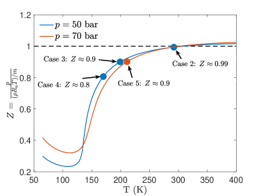
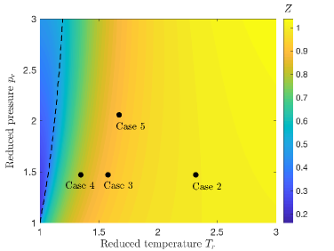
(a)                      (b)

Figure 1: (a) Compressibility factor of $\mathrm{N_{2}}$ at $50$ and $70$ bar pressure. Blue and red markers denote the ambient conditions for various high-$p$ cases of table 2. (b) $p$-$T$ diagram of $\mathrm{N_{2}}$ at supercritical conditions. The reduced temperature is $T_{r}=T/T_{c}$ and the reduced pressure is $p_{r}=p/p_{c}$, where the critical temperature $T_{c}=126.2~{}$K and critical pressure $p_{c}=33.98~{}$bar for $\mathrm{N_{2}}$. The contour illustrates the distribution of $Z$ and the black dashed line is the Widom line defined as the locus of the maximum isobaric heat capacity. Black markers denote the location of various high-$p$ cases of table 2 on the thermodynamic state plane.

Case (description)	$Z$	$\beta_{T}\times 10^{5}$	$p_{\infty}\left(\beta_{T}-\frac{1}{p_{\infty}}\right)$	$\gamma$	$\beta_{S}\times 10^{5}$
		$\left(\mathrm{Pa}^{-1}\right)$			$\left(\mathrm{Pa}^{-1}\right)$
1 (atm-$p$)	1	1.00000	0.000	1.4	0.71429
2 (high-$p\left(50\right)$; $Z\approx 1$)	0.99	0.01995	-0.002	1.49	0.01339
3 (high-$p\left(50\right)$; $Z\approx 0.9$)	0.9	0.02190	0.095	1.69	0.01296
4 (high-$p\left(50\right)$; $Z\approx 0.8$)	0.8	0.02488	0.244	1.96	0.01269
5 (high-$p\left(70\right)$; $Z\approx 0.9$)	0.9	0.01524	0.067	1.74	0.00876

Table 3: Values of various thermodynamic quantities for ambient conditions in Cases 1 to 5. Cases 2M and 4M have same values as Cases 2 and 4, respectively, and Cases 1T, 2T and 4T have same values as Cases 1, 2 and 4, respectively.

2.1 Conservation equations

The compressible flow equations for conservation of mass, momentum, energy, and a passive scalar, solved in this study, are

$$\frac{\partial\rho}{\partial t}+\frac{\partial}{\partial x_{j}}\left[\rho u_{j}\right]=0,$$ (4)

$$\frac{\partial}{\partial t}\left(\rho u_{i}\right)+\frac{\partial}{\partial x_{j}}\left[\rho u_{i}u_{j}+p\delta_{ij}-\sigma_{ij}\right]=0,$$ (5)

$$\frac{\partial}{\partial t}\left(\rho e_{t}\right)+\frac{\partial}{\partial x_{j}}\left[\left(\rho e_{t}+p\right)u_{j}-u_{i}\sigma_{ij}+q_{j}\right]=0,$$ (6)

$$\frac{\partial}{\partial t}\left(\rho\xi\right)+\frac{\partial}{\partial x_{j}}\left[\rho\xi\ u_{j}+J_{j}\right]=0,$$ (7)

where $t$ denotes the time, $\left(x_{1},x_{2},x_{3}\right)\equiv\left(x,y,z\right)$ are the Cartesian directions, subscripts $i$ and $j$ refer to the spatial coordinates, $u_{i}$ is the velocity, $p$ is the pressure, $\delta_{ij}$ is the Kronecker delta, $e_{t}=e+u_{i}u_{i}/2$ is the total energy (i.e., internal energy, $e$, plus kinetic energy), $\xi\in\left[0,1\right]$ is a passive scalar transported with the flow, $\sigma_{ij}$ is the Newtonian viscous stress tensor

$$\sigma_{ij}=\mu\left(2S_{ij}-\frac{2}{3}S_{kk}\delta_{ij}\right),\qquad S_{ij}=\frac{1}{2}\left(\frac{\partial u_{i}}{\partial x_{j}}+\frac{\partial u_{j}}{\partial x_{i}}\right),$$ (8)

where $\mu$ is the viscosity, $S_{ij}$ is the strain-rate tensor, and $q_{j}=-\lambda\thinspace\partial T/\partial x_{j}$ and $J_{j}=-\mathscr{D}\thinspace\partial\xi/\partial x_{j}$ are the heat flux and scalar diffusion flux in $j$-direction, respectively. $\lambda$ is the thermal conductivity and $\mathscr{D}=\mu/Sc$ is the scalar diffusivity, where $Sc$ denotes the Schmidt number. The injected fluid is assigned a scalar value, $\xi$, of 1, whereas the chamber fluid a value of 0. The passive scalar is not a physical species, and is only used as a surrogate quantity to track the injected fluid in this simple single-species flow.

2.2 Equation of state

For the near-atmospheric-$p$ simulations (Cases 1 and 1T), the perfect gas equation of state (EOS) is applicable, given by

$$p=\frac{\rho R_{\mathrm{u}}T}{m}.$$ (9)

For the high-$p$ simulations (Cases 2–5, 2M, 4M, 2T and 4T), the conservation equations are coupled with a Peng-Robinson (PR) EOS

$$p=\frac{R_{\mathrm{u}}T}{\left(v_{\mathrm{PR}}-b_{\mathrm{mix}}\right)}-\frac{a_{\mathrm{mix}}}{\left(v_{\mathrm{PR}}^{2}+2b_{\mathrm{mix}}v_{\mathrm{PR}}-b_{\mathrm{mix}}^{2}\right)}.$$ (10)

The molar PR volume $v_{\mathrm{PR}}=V-v_{\mathrm{s}}$, where the molar volume $V=m/\rho$. $v_{\mathrm{s}}$ denotes the volume shift introduced to improve the accuracy of the PR EOS at high pressures Okong’o et al. (2002); Harstad et al. (1997). $a_{mix}$ and $b_{mix}$ are functions of $T$ and the molar fraction $X_{\alpha}$ – here $X_{\alpha}=1$ – and are obtained from expressions previously published (Sciacovelli & Bellan, 2019, Appendix B).

2.3 Transport properties

For the near-atmospheric-$p$ simulations (Cases 1 and 1T), the viscosity is modeled as a power law

$$\mu=\mu_{R}\left(\frac{T}{T_{R}}\right)^{n}$$ (11)

with $n=2/3$ and the reference viscosity being $\mu_{R}=\rho_{e}U_{e}D/Re_{D}$, where $\rho_{e}$ and $U_{e}$ are the jet-exit fluid density and jet-exit bulk velocity, respectively, and the reference temperature is $T_{R}=293\thinspace\mathrm{K}$. The thermal conductivity is $\lambda=\mu C_{p}/\mathrm{Pr}$, where Prandtl number $\mathrm{Pr}=0.7$ (as typical of 1 bar flows), the ratio of specific heats $\gamma=1.4$, and the isobaric heat capacity $C_{p}=\gamma R_{\mathrm{u}}/\left(\gamma-1\right)$ is assumed.

For real gases in high-$p$ simulations (Cases 2–5, 2M, 4M, 2T and 4T), the physical viscosity, $\mu_{\mathrm{ph}}$, and thermal conductivity, $\lambda_{\mathrm{ph}}$, are calculated using the Lucas method (Poling et al., 2001, Chapter 9) and the Stiel-Thodos method (Poling et al., 2001, Chapter 10), respectively, as a function of the local thermodynamic conditions. The computational viscosity, $\mu$, and thermal conductivity, $\lambda$, are obtained by scaling $\mu_{\mathrm{ph}}$ and $\lambda_{\mathrm{ph}}$ with a factor $\mathcal{F}=\mu_{R}/\mu_{\mathrm{ph},\infty}$, i.e. $\mu=\mathcal{F}\mu_{\mathrm{ph}}$ and $\lambda=\mathcal{F}\lambda_{\mathrm{ph}}$, to allow simulations at the specified $Re_{D}$ of 5000. The ambient physical viscosity ($\mu_{\mathrm{ph},\infty}$) is $\mu_{\mathrm{ph}}$ at the pressure $p_{\infty}$ and the temperature $T_{\mathrm{ch}}$ of respective cases. This procedure ensures that $\mathrm{Pr}$, which is computed as a function of the local thermodynamic variables, has the physically correct value. The scalar diffusivity is obtained from $\mathscr{D}=\mu/Sc$, where unity Schmidt number is assumed in all cases. A validation of the transport and thermodynamic properties calculated from the above methods is presented in Appendix A.

The $\mathcal{F}$ values for all cases are listed in table 2. As an example, for Case 1, $\mathcal{F}=\mu_{R}/\mu_{\mathrm{ph},\infty}\approx 6.5$ ($\mu_{R}=\rho_{e}U_{e}D/\operatorname{Re}_{D}=1.136\times 10^{-4}\,\mathrm{Pa.s}$ and $\mu_{\mathrm{ph},\infty}=1.757\times 10^{-5}\,\mathrm{Pa.s}$ at $p_{\infty}=1\,$bar and $T_{\mathrm{ch}}=293\,$K), and for Case 2, $\mathcal{F}\approx 309.4$ ($\mu_{R}=5.715\times 10^{-3}\,\mathrm{Pa.s}$ and $\mu_{\mathrm{ph},\infty}=1.847\times 10^{-5}\,\mathrm{Pa.s}$ at $p_{\infty}=50\,$bar and $T_{\mathrm{ch}}=293\,$K). $\mathcal{F}$ is larger in Case 2 compared to Case 1 because of the larger density $\rho_{e}$ at $50$ bar that requires a larger $\mu_{R}$ for a fixed $\operatorname{Re}_{D}$, while the physical viscosity $\mu_{\mathrm{ph},\infty}$ remains relatively unchanged with increase in $p$.

3 Numerical aspects

3.1 Computational domain and numerical method

For notation simplicity, $\left(x_{1},x_{2},x_{3}\right)\equiv\left(x,y,z\right)$ is adopted for axis labels. $\left(u_{1},u_{2},u_{3}\right)$ denote the Cartesian velocity components, whereas $\left(u,v,w\right)$ denote the axial, radial and azimuthal velocity. The computational domain extends to $42D$ in the axial ($x$-)direction and $20D$ in the $y$- and $z$-direction including the sponge zones, as shown schematically in a $x$-$z$ plane of figure 2. The boundary conditions are discussed in §3.2.1.

Spatial derivatives are approximated using the sixth-order compact finite-difference scheme and time integration uses the classical explicit fourth-order Runge-Kutta method. To avoid unphysical accumulation of energy at high wavenumbers, resulting from the use of non-dissipative spatial discretization, the conservative variables are filtered every five time steps using an explicit eighth-order filter Kennedy & Carpenter (1994). The derivative approximations and filter operations over non-uniform stretched grids and polar grids (for post-processing and inflow generation) uses the generalized-coordinate formulation (e.g. Sharan, 2016; Sharan et al., 2018b).

To obtain the numerical solution, the conservation equations are first solved at each time step. With $\rho$ and $e=e_{t}-u_{i}u_{i}/2$ obtained from the conservation equations and $T$ computed iteratively from $e,$ the EOS is used to calculate $p$ Okong’o et al. (2002).

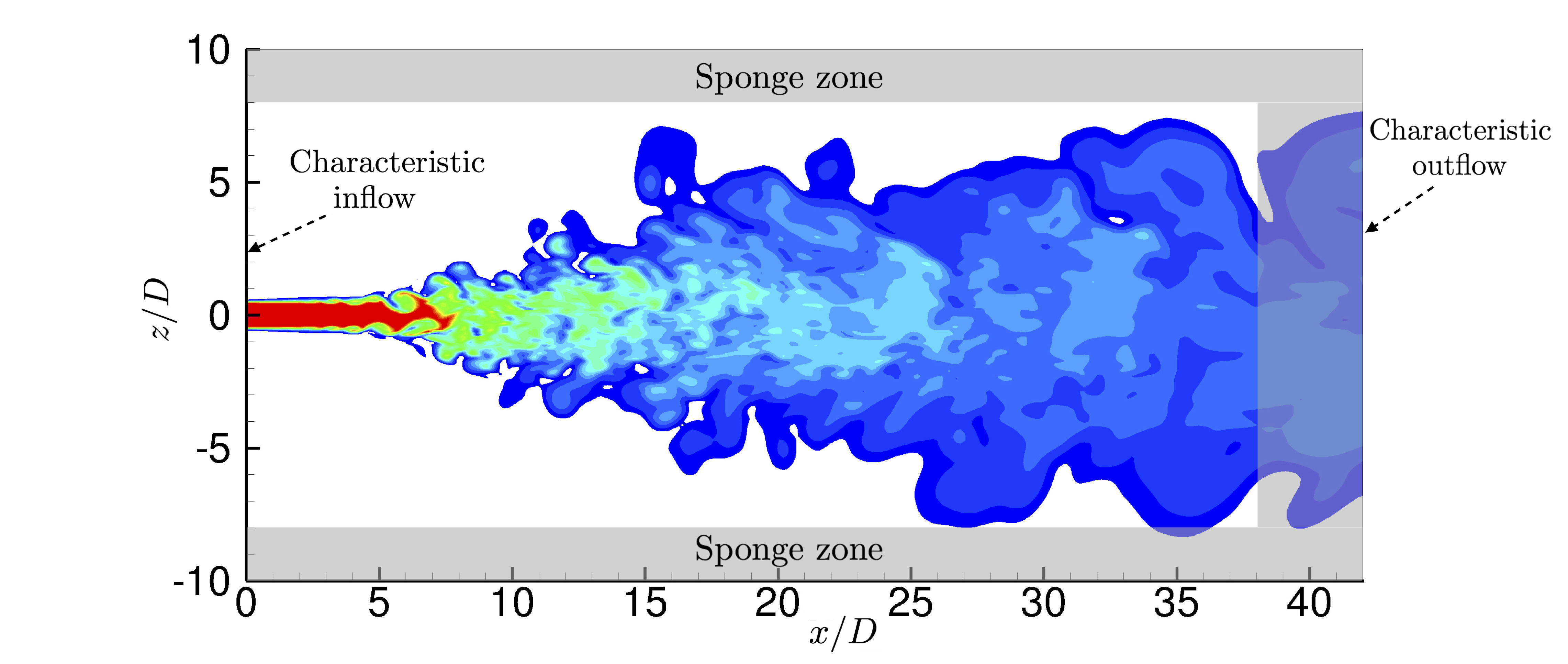
Figure 2: A 2D schematic showing the extent of computational domain in axial and radial direction, and the boundary conditions applied at various boundaries.

3.2 Boundary and inflow conditions

3.2.1 Boundary conditions

The outflow boundary in the axial direction and all lateral boundaries have sponge zones Bodony (2006) with non-reflecting outflow Navier-Stokes characteristic boundary conditions (NSCBC) Poinsot & Lele (1992) at the boundary faces. Sponge zones at each outflow boundary have a width of $10\%$ of the domain length normal to the boundary face. The sponge strength at each boundary decreases quadratically with distance normal to the boundary. The performance of one-dimensional NSCBC Poinsot & Lele (1992); Okong’o & Bellan (2002a) as well as its three-dimensional extension Lodato et al. (2008) by inclusion of transverse terms were also evaluated without the sponge zones; they permit occasional spurious reflections into the domain and, therefore, the use of sponge zones was deemed necessary.

3.2.2 Inflow conditions

The role of initial/inflow conditions on free-shear flow development as well as the asymptotic (self-similar) state attained by the flow at atmospheric conditions is well recognized George & Davidson (2004); Boersma et al. (1998); Sharan et al. (2019). To examine the high-$p$ jet-flow sensitivity to initial conditions, two types of inflows are considered, portraying either a jet exiting a smooth contracting nozzle or a jet exiting a long pipe. The former produces laminar inflow conditions with top-hat jet-exit mean velocity profile whereas the latter produces turbulent inflow conditions of fully-developed pipe flow Mi et al. (2001).

Cases 1–5, 2M and 4M employ laminar inflow conditions with velocity profile at the inflow plane given by (e.g. Michalke, 1984)

$$u(r)=\frac{U_{e}}{2}\left(1-\tanh\left[\frac{r-r_{0}}{2\theta_{0}}\right]\right),$$ (12)

where $r=\sqrt{y^{2}+z^{2}}$, the jet exit radius is $r_{0}=D/2$ and the momentum thickness is $\theta_{0}=0.04r_{0}$. Small random perturbations with maximum amplitude of $0.004U_{e}$, as listed in table 2, are superimposed on the inflow velocity profile to trigger jet flow transition to turbulence. Perturbations are only added to the velocity field.

Cases 1T, 2T and 4T utilize turbulent inflow conditions, typical of jets exiting a long pipe. The inflow is generated using the approach of Klein et al. (2003) modified to accommodate circular-pipe inflow geometry. This approach generates inflow statistics matching a prescribed mean velocity and Reynolds stress tensor, using the method of Lund et al. (1998), with fine-scale perturbations possessing a prescribed spatial correlation length scale. The mean velocity and Reynolds stress profiles are here specified from the fully-developed pipe flow DNS results of Eggels et al. (1994), where the Reynolds number, based on pipe diameter and bulk velocity, of $5300$ is close to the jet Reynolds number of present study. The bulk velocity is defined as

$$U_{b}=\frac{1}{\pi\left(D/2\right)^{2}}\stackrel{{\scriptstyle[}}{{0}}]{D/2}{\int}2\pi ru\thinspace\mathrm{d}r.$$ (13)

For small values of $\theta_{0}$ in (12), $U_{b}$ for laminar inflow cases is approximately equal to $U_{e}$. $U_{b}$ in Cases 1T, 2T and 4T is chosen to be equal to $U_{e}$ of Cases 1, 2 and 4, respectively, to allow fair one-to-one comparisons between them. Since $U_{e}$ has the same value for Cases 1–5, the bulk inflow velocity is approximately the same for Cases 1–5, 1T, 2T and 4T. The choice of the correlation length scale determines the energy distribution among various spatial scales. Increasing the length scale leads to more dominant large-scale structures. Since the turbulent inflow simulations are aimed at examining the influence of fully-developed fine-scale inflow turbulence on jet statistics, a small isotropic value of $L/D=0.1$ is assumed for the correlation length scale, this value being marginally larger than the finest scale in the velocity spectra of figures 7(a-c) in Eggels et al. (1994).

Figures 3 and 4 validate the turbulent inflow implementation. In figure 3, the mean axial velocity from the present turbulent inflow is compared against the pipe flow DNS results (case DNS(E) of Eggels et al., 1994). Figure 4 illustrates a similar comparison of the r.m.s. axial-velocity fluctuation, $u^{\prime}_{\textrm{rms}}$, and the Reynolds stress, $\overline{u^{{}^{\prime}}v^{{}^{\prime}}}$. The radial- and the azimuthal-velocity fluctuations, $v^{\prime}_{\textrm{rms}}$ and $w^{\prime}_{\textrm{rms}}$, compare similarly well with the respective DNS profiles, and have been omitted for brevity. The overbar $\left(\bar{\bullet}\right)$ denotes mean quantities, calculated by an average over time and azimuthal ($\theta$) coordinate, given by a discrete approximation of

$$\bar{u}(x,r)=\frac{1}{2\pi}\intop_{0}^{2\pi}\left(\frac{1}{\left(t_{2}-t_{1}\right)}\intop_{t_{1}}^{t_{2}}u(x,r,\theta,t)\mathrm{d}t\right)\mathrm{d}\theta.$$ (14)

For all results in this study, the time average is performed over time steps in the interval $t_{1}=1000\leq tU_{e}/D\leq 4000=t_{2}$. The r.m.s. fluctuations are calculated from

$$u^{\prime}_{\mathrm{rms}}=\sqrt{\left\langle\left\langle\left(u-\left\langle u\right\rangle_{t}\right)^{2}\right\rangle_{t}\right\rangle_{\theta}}=\sqrt{\left\langle\left\langle u^{2}\right\rangle_{t}-\left\langle u\right\rangle_{t}^{2}\right\rangle_{\theta}},$$ (15)

where $\left\langle\cdot\right\rangle_{t}$ and $\left\langle\cdot\right\rangle_{\theta}$ denotes the time and azimuthal averages, respectively. Using the notation $\left\langle\cdot\right\rangle_{t}$ and $\left\langle\cdot\right\rangle_{\theta}$, (14) can be written as $\bar{u}=\left\langle\left\langle u\right\rangle_{t}\right\rangle_{\theta}$.

The method described in Klein et al. (2003) assumes a Cartesian grid with uniform spacing, where the periodic directions, along which averages are computed to determine mean quantities, are aligned with the Cartesian directions. The round-jet inflow considered here has circular orifice, where the azimuthal direction is periodic, which is not aligned with a Cartesian direction. Therefore, the fluctuations are computed on a polar grid and, then, interpolated to the Cartesian inflow grid.

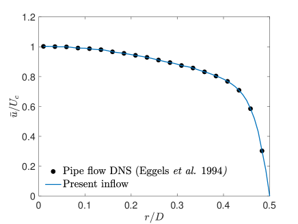
Figure 3: Inflow mean velocity normalized by the centerline velocity for the (pseudo-)turbulent inflow compared against the pipe flow DNS results of Eggels et al. (1994).

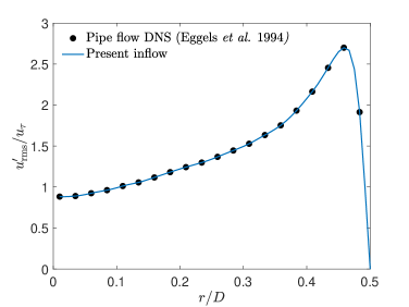
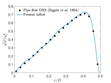
(a)                        (b)

Figure 4: (a) R.m.s. axial velocity fluctuation, $u^{\prime}_{\textrm{rms}}$, and (b) the Reynolds stress, $\overline{u^{{}^{\prime}}v^{{}^{\prime}}}$, normalized by the wall friction velocity, $u_{\tau}$, from the (pseudo-)turbulent inflow compared against the pipe flow DNS results of Eggels et al. (1994).

4 Results

The influence of $p_{\infty}$ and $Z$ on the laminar-inflow jet behavior is examined first in §4.1. Then, the effects of $p_{\infty}$ at a fixed $Z$ of 0.9 are investigated in §4.2. To differentiate between the effects of dynamic and thermodynamic compressibility, the influence of $p_{\infty}$ and $Z$ at a fixed $Ma_{e}$ of 0.6 is studied in §4.3. Finally, the effect of the inflow condition – laminar versus turbulent – is addressed in §4.4, first as a baseline for the fully compressible atmospheric-$p$ conditions in §4.4.1 and then at high-$p$ conditions in §4.4.2.

To provide confidence in the numerical formulation and discretization, a validation of Case 1, which obeys the perfect-gas EOS, against experimental results is presented in Appendix C; additionally, those results permit comparisons with high-$p$ flow results where relevant.

4.1 Effects of high pressure and compressibility factor

The influence of $p_{\infty}$ (from atmospheric to supercritical) on jet-flow dynamics and mixing is here examined by comparing results from Cases 1 and 2. Further, the effects of $Z$ at supercritical $p_{\infty}$ are examined by comparing results from Cases 2 to 4. As indicated in table 2, in each case the fluid in the injected jet is as dense as the ambient (or chamber) fluid. The inflow bulk velocity, defined by (13), is the same for all cases. As a result, the inflow bulk momentum varies with change in inflow density.

4.1.1 Mean axial velocity and spreading rate

The inverse of the centerline mean axial velocity, $U_{c}(x)$ $\left(=\bar{u}(x,0)\right)$, normalized by the the jet-exit centerline velocity, $U_{0}$ $\left(=U_{c}(0)\right)$, for Cases 1 to 4 is presented in figure 5(a). For the laminar inflow cases, which have a top-hat jet-exit mean velocity profile, $U_{0}=U_{e}$, and since Cases 1–5 use same $U_{e}$, $U_{0}$ is the same for all cases in figure 5(a). To our knowledge, figure 5(a) demonstrates for the first time that supercritical jets in the Mach number range $\left[0.58,\thinspace 0.82\right]$, see table 2, attain self-similarity. This finding differs from the self-similarity observed in the low-Mach-number results of Ries et al. (2017), where the compressibility effects were ignored and the conservation equations did not use the pressure calculated from the EOS. In contrast, the fully compressible equations solved in the present study use the strongly non-linear EOS which contributes to the thermodynamic-variable fluctuations, and self-similarity is not an obvious outcome.

In figure 5(a), the potential core length is approximately the same in all cases, but the velocity decay rates differ among cases in both the transition and the fully-developed self-similar regions. In the transition region ($7\lesssim x/D\lesssim 15$), the mean axial-velocity decay, assessed by the slope of the lines in figure 5(a), decreases with increasing $p_{\infty}$ from $1$ bar (Case 1) to $50$ bar (Case 2), remains approximately the same with decrease in $Z$ from $0.99$ (Case 2) to $0.9$ (Case 3), and increases significantly with further decrease in $Z$ to $0.8$ (Case 4). In the self-similar region, the decay rates are quantified by the inverse of $B_{u}$, defined through equation (19). $1/B_{u}$ increases from $1/5.5$ for Case 1 to $1/5.4$ for Case 2 & 3 and to $1/4.4$ for Case 4. Lines with slope $1/B_{u}$ are shown as black dashed lines in figure 5(a).

Figure 5(b) compares the velocity half-radius ($r_{\frac{1}{2}u}$) among Cases 1–4. In the transition region ($7\lesssim x/D\lesssim 15$), the jet spread defined by the half-radius is larger for Case 1 than Case 2. The profiles are nearly identical for Cases 2 and 3, and Case 4 shows a significantly larger jet spread than the other cases. In the self-similar region, the linear spread can be described by the black solid lines of figure 5(b); the equations describing the solid lines are included in the figure caption. The self-similar spread rate decreases from Case 1 to Case 4. The decrease is relatively small from Case 2 to Case 3, and negligible from Case 3 to Case 4. Variation of $\xi_{c}/\xi_{0}$ and $r_{\frac{1}{2}\xi}/D$ (not shown here for brevity) are similar to those of the velocity field in figure 5.

The decay of $U_{c}$, observed in figure 5(a), is a result of the concurrent processes of: (a) transfer of kinetic energy from the mean field to fluctuations, (b) transport of mean kinetic energy away from the centerline as more ambient fluid is entrained, and (c) mean viscous dissipation. These processes interact as follows. The entrainment of ambient fluid (initially at rest) into the jet enhances the momentum and kinetic energy of the ambient fluid. Transport of momentum/energy from the jet core facilitates the ambient-fluid entrainment and jet spread. As a result, a wider jet spread is associated with a larger decay in $U_{c}$. Therefore, the profiles for various cases look similar in figures 5(a) and (b). Production term of the t.k.e. equation quantifies the loss of mean kinetic energy to turbulent fluctuations and mean strain rate magnitude is proportional to the mean viscous dissipation. The variation of $U_{c}$ across various cases in figure 5(a) follows the variation of t.k.e. production and mean strain rate magnitude, as discussed in §4.4.2.5.

The considerably larger decay of $U_{c}$ in Case 4 compared to other cases is at this point conjectured to be a coupled effect of its proximity to the Widom line, i.e. the thermodynamic state (see figure 1), and the mean strain rates generated in the flow, i.e. the dynamic state, that depends on the thermodynamic state, the inflow condition (laminar versus turbulent), and the jet-exit (inflow) Mach number. The proximity to the Widom line determines the departure from perfect-gas behavior and the relative magnitude of pressure fluctuations across various cases, as further discussed in §4.1.3. Prior to examining the role of pressure flucutations in the unique behavior of Case 4, an evaluation of the consistency of $U_{c}$ decay with the kinetic energy transfer from the mean field to fluctuations is performed by next examining the velocity fluctuations and their self-similarity.

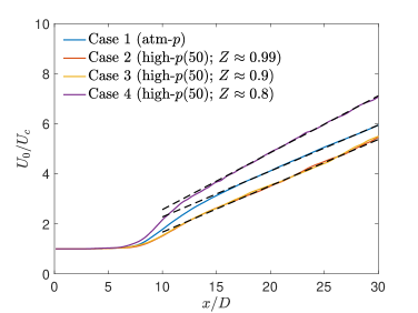
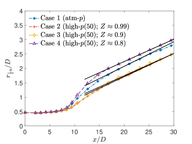
(a)                        (b)

Figure 5: Case 1–4 comparisons: Streamwise variation of the (a) inverse of centerline mean axial velocity ($U_{c}$) normalized by the jet-exit centerline velocity ($U_{0}$) and (b) velocity half radius ($r_{\frac{1}{2}u}$). The black dashed lines in (a) are given by equation (19) using $B_{u}=5.5$, $x_{0u}=-2.4D$ for Case 1, $B_{u}=5.4$, $x_{0u}=D$ for Cases 2 & 3, and $B_{u}=4.4$, $x_{0u}=-1.3D$ for Case 4. The black solid lines in (b) are given by: $r_{\frac{1}{2}u}/D=0.085\left(x/D+4.4\right)$ for Case 1, $r_{\frac{1}{2}u}/D=0.0805\left(x/D+1.3\right)$ for Case 2, $r_{\frac{1}{2}u}/D=0.0775\left(x/D+2.5\right)$ for Case 3, and $r_{\frac{1}{2}u}/D=0.077\left(x/D+8.9\right)$ for Case 4.

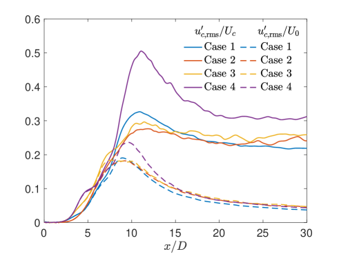
Figure 6: Case 1–4 comparisons: Streamwise variation of the centerline r.m.s. axial-velocity fluctuation ($u^{\prime}_{c,\textrm{rms}}$) normalized by the centerline mean value, $U_{c}$, and jet-exit mean value, $U_{0}$.

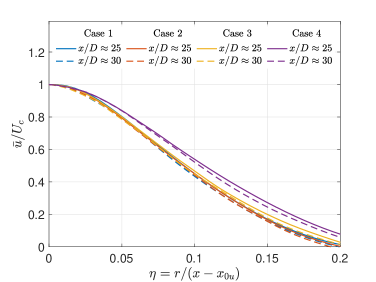
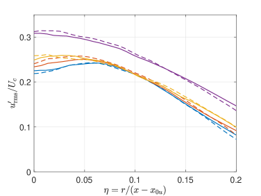
(a)                        (b)

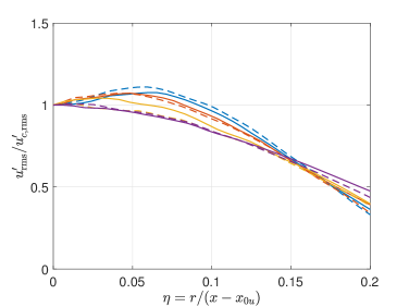
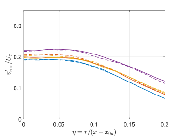
(c)                        (d)

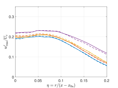
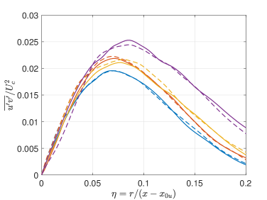
(e)                        (f)

Figure 7: Case 1–4 comparisons: Radial profiles of (a) mean axial velocity ($\bar{u}$) normalized by the centerline mean axial velocity ($U_{c}$), (b) r.m.s. axial velocity fluctuations ($u_{\mathrm{rms}}^{{}^{\prime}}$) normalized by the centerline mean axial velocity, (c) r.m.s. axial velocity fluctuations ($u_{\mathrm{rms}}^{{}^{\prime}}$) normalized by the centerline r.m.s. axial velocity fluctuations ($u_{c,\mathrm{rms}}^{{}^{\prime}}$), (d) normalized r.m.s. radial velocity fluctuations ($v_{\mathrm{rms}}^{{}^{\prime}}$), (e) normalized r.m.s. azimuthal velocity fluctuations ($w_{\mathrm{rms}}^{{}^{\prime}}$), and (f) normalized Reynolds stress ($\overline{u^{{}^{\prime}}v^{{}^{\prime}}}$) at various axial locations. The legend is the same for all plots.

4.1.2 Velocity fluctuations and self-similarity

The centerline r.m.s. axial-velocity fluctuation is depicted in figure 6 for Cases 1–4 with two different normalizations. Since $U_{0}$ has the same value for Cases 1–4, the normalization with $U_{0}$ compares the absolute fluctuation magnitude among various cases. On the other hand, the normalization with $U_{c}$ shows the fluctuation magnitude with respect to the local mean value. Larger $u^{\prime}_{c,\textrm{rms}}/U_{c}$ values are expected to indicate greater local transfer of mean kinetic energy to fluctuations. Accordingly, larger $u^{\prime}_{c,\textrm{rms}}/U_{c}$ in figure 6 should imply a higher slope ($U_{c}$ decay rate) in the corresponding region in figure 5(a). Case 4, which has the largest $u^{\prime}_{c,\textrm{rms}}/U_{c}$ among all cases in both the transition and the self-similar region, also exhibits largest slopes (decay rates) in figure 5(a). Case 1 has larger $u^{\prime}_{c,\textrm{rms}}/U_{c}$ than Cases 2 and 3 in the transition region, and, accordingly, higher decay rates in that region in figure 5(a). In the self-similar region, $u^{\prime}_{c,\textrm{rms}}/U_{c}$ in Cases 2 and 3 are marginally larger than in Case 1, and, accordingly, the self-similar $U_{c}$ decay rates of Cases 2 and 3 are marginally higher. This confirms that the decay in $U_{c}$ is consistently reflected in the magnitude of $u^{\prime}_{c,\textrm{rms}}/U_{c}$.

The linear mean axial-velocity decay and the linear jet-spread rate, downstream of the transition region, in figure 5 indicates the self-similarity of the mean axial velocity. The self-similarity of mean axial velocity and Reynolds stresses is further examined from their radial variation in figure 7. Figure 7(a) shows the radial profiles of $\bar{u}/U_{c}$ from Cases 1–4 at $x/D\approx 25$ (solid lines) and $30$ (dashed lines). In all cases, profiles at the two axial locations show minimal differences, suggesting that $\bar{u}/U_{c}$ has attained self-similarity. The self-similar mean velocity/scalar profile is commonly expressed as (e.g. Mi et al., 2001; Xu & Antonia, 2002)

$$\bar{u}(x,r)=U_{c}\left(x\right)f\left(\eta\right),\qquad\bar{\xi}(x,r)=\xi_{c}\left(x\right)g\left(\eta\right),$$ (16)

where $f\left(\eta\right)$ and $g\left(\eta\right)$ are similarity functions, often described by Gaussian distributions,

$$f\left(\eta\right)=\exp\left(-A_{u}\eta^{2}\right),\qquad g\left(\eta\right)=\exp\left(-A_{\xi}\eta^{2}\right),$$ (17)

where $A_{u}$ and $A_{\xi}$ are constants, here determined from a least-squares fit of the simulation data. The least-squares procedure applied to $x/D\approx 30$ profiles of figure 7(a) yields $A_{u}=79.5$ for Cases 1 and 2, $A_{u}=77.2$ for Case 3, and $A_{u}=64.4$ for Case 4. Thus, increasing $p$ from $1$ bar (Case 1) to $50$ bar (Case 2) has minimal influence on the radial variation of the self-similar axial-velocity profile. A decrease in $Z$ from $0.99$ (Case 2) to $0.9$ (Case 3) and then to $0.8$ (Case 4) at $p_{\infty}=50$ bar increases $\bar{u}/U_{c}$ at a fixed $\eta$.

The radial variation of normalized r.m.s. velocity fluctuations at $x/D\approx 25$ and $30$ are compared for Cases 1–4 in figures 7(b)–(e). In all figures, the profiles at $x/D\approx 25$ (solid lines) and $30$ (dashed lines) show minimal difference, and hence the r.m.s. velocity fluctuations can be considered self-similar around $x/D\approx 25$. $u^{\prime}_{\textrm{rms}}/U_{c}$, shown in figure 7(b), increases in the vicinity of centerline with increase in $p_{\infty}$ from $1$ bar (Case 1) to $50$ bar (Case 2), but the differences diminish with increase in $\eta$. A decrease in $Z$ from $0.99$ (Case 2) to $0.9$ (Case 3) marginally increases $u^{\prime}_{\textrm{rms}}/U_{c}$ at both small and large $\eta$. Further decrease in $Z$ from $0.9$ (Case 3) to $0.8$ (Case 4) shows significant increase in $u^{\prime}_{\textrm{rms}}/U_{c}$ at all $\eta$-locations. $u^{\prime}_{\textrm{rms}}/u^{\prime}_{c,\textrm{rms}}$, plotted in figure 7(c) shows that the fluctuations increase with radial distance near the centerline in Case 1, with maximum at $\eta\approx 0.07$. The location of the maximum (in terms of $\eta$) recedes towards the centerline progressively in Cases 2 and 3. Case 4 does not exhibit an off-axis maximum and $u^{\prime}_{\textrm{rms}}/u^{\prime}_{c,\textrm{rms}}$ decreases monotonically with $\eta$, highlighting the peculiarity with respect to Cases 2 and 3.

Additionally, $v_{\textrm{rms}}^{\prime}/U_{c}$ and $w_{\text{rms}}^{\prime}/U_{c}$, shown in figures 7(d) and (e), respectively, increase from Case 1 to 4. The increase is marginal from Case 1 to 3, but significant in Case 4. Axisymmetry of a round-jet flow requires that $v^{\prime}_{\textrm{rms}}$ and $w^{\prime}_{\textrm{rms}}$ be equal at the centerline, which is nearly true for all cases in figures 7(d) and (e). Comparable profiles of $\overline{u^{\prime}v^{\prime}}/U_{c}^{2}$ in figure 7(f) at $x/D\approx 25$ and $30$ suggest that $\overline{u^{\prime}v^{\prime}}/U_{c}^{2}$ attains self-similarity around $x/D\approx 25$ in Cases 1–4. $\overline{u^{\prime}v^{\prime}}/U_{c}^{2}$ is similar for Cases 1–4 in the vicinity of the centerline but the profiles differ at larger $\eta$, where Case 4 values are considerably larger than the other cases.

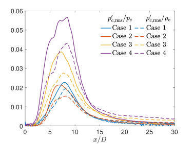
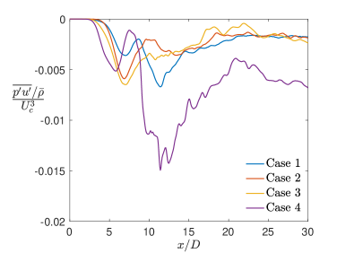
(a)                        (b)

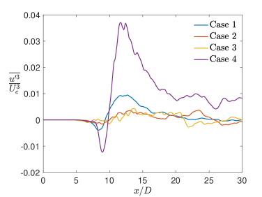
(c)

Figure 8: Case 1–4 comparisons: Streamwise variation of the (a) centerline r.m.s. pressure and density fluctuations, denoted by $p^{\prime}_{c,\mathrm{rms}}$ and $\rho^{\prime}_{c,\mathrm{rms}}$, respectively, normalized by the centerline mean pressure ($p_{c}$) and density ($\rho_{c}$), respectively, (b) normalized fluctuating pressure-axial velocity correlation $\left(\overline{p^{\prime}u^{\prime}}/\bar{\rho}U_{c}^{3}\right)$, and (c) normalized third-order velocity moment $\left(\overline{u^{\prime 3}}/U_{c}^{3}\right)$.

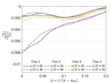
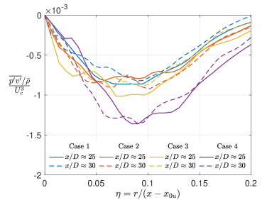
(a)                        (b)

Figure 9: Case 1–4 comparisons: Radial profiles of the (a) normalized pressure-axial velocity correlation and (b) normalized pressure-radial velocity correlation at $x/D\approx 25$ and $30$.

4.1.3 Pressure and density fluctuations, pressure-velocity correlation, and third-order velocity moments

The differences in mean axial-velocity for various cases, observed in figure 5, is consistent with the differences in velocity fluctuations, examined in the previous section. Larger velocity fluctuations imply greater transfer of energy from the mean field to fluctuations, resulting in greater decay of mean velocity. The differences in velocity fluctuations with $p_{\infty}$ and $Z$, however, remain to be explained, and this topic is addressed next.

Gradients of the pressure/density fluctuations, pressure-velocity correlations and third-order velocity moments determine the transport terms in the Reynolds stress and t.k.e. equations (e.g. Panchapakesan & Lumley, 1993; Hussein et al., 1994), and hence their role in causing the differences observed in velocity fluctuations of Cases 1–4 (figures 6 and 7) is examined in figures 8, 9, and 10.

The axial variation of the centerline r.m.s. pressure and density fluctuations normalized using centerline mean values, $p_{c}$ and $\rho_{c}$, respectively, are compared in figure 8(a) for Cases 1–4. The normalization provides information on the fluctuation magnitude with respect to local pressure and density (thermodynamic state). In all cases, $p^{\prime}_{c,\textrm{rms}}/p_{c}$ and $\rho^{\prime}_{c,\textrm{rms}}/\rho_{c}$ have a maximum in the transition region and asymptote to a constant value in the self-similar region. $p^{\prime}_{c,\textrm{rms}}/p_{c}$ exceed $\rho^{\prime}_{c,\textrm{rms}}/\rho_{c}$ in the transition region and vice versa in the self-similar region. Increasing $p_{\infty}$ from $1$ bar (Case 1) to $50$ bar (Case 2) slightly reduces $p^{\prime}_{c,\textrm{rms}}/p_{c}$ (shown as solid lines) and $\rho^{\prime}_{c,\textrm{rms}}/\rho_{c}$ (shown as dashed lines) at all centerline locations, whereas decreasing $Z$ from $0.99$ (Case 2) to $0.9$ (Case 3) and then to $0.8$ (Case 4) increases $p^{\prime}_{c,\textrm{rms}}/p_{c}$ and $\rho^{\prime}_{c,\textrm{rms}}/\rho_{c}$ significantly. The variation of $p^{\prime}_{c,\textrm{rms}}/p_{c}$ and $\rho^{\prime}_{c,\textrm{rms}}/\rho_{c}$ follows the variation of $p_{\infty}\left(\beta_{T}-1/p_{\infty}\right)$, listed in table 3, that measures the real-gas effects at ambient thermodynamic condition. The large value of $p_{\infty}\left(\beta_{T}-1/p_{\infty}\right)$ for Case 4 concurs with the large $p^{\prime}_{c,\textrm{rms}}/p_{c}$ and $u^{\prime}_{c,\textrm{rms}}/U_{c}$ observed in Case 4, a fact which indicates that the large $U_{c}$ decay and jet spread in Case 4 is a result of the real-gas effects due to its proximity to the Widom line.

While $p_{\infty}\left(\beta_{T}-1/p_{\infty}\right)$ explains the behavior of Case 4 with respect to other cases, it does not explain the behavior of Case 3 with respect to Case 1 in the transition region of the flow. Larger $p_{\infty}\left(\beta_{T}-1/p_{\infty}\right)$ in Case 3 may suggest larger $p^{\prime}_{c,\textrm{rms}}/p_{c}$ and $u^{\prime}_{c,\textrm{rms}}/U_{c}$ in Case 3 compared to Case 1. But, while $p^{\prime}_{c,\textrm{rms}}/p_{c}$ is larger in Case 3 than in Case 1 at all axial locations, $u^{\prime}_{c,\textrm{rms}}/U_{c}$ in Case 1 exceeds Case 3 in the transition region resulting in larger $U_{c}$ decay and jet spread in Case 1 than in Case 3. To understand this discrepancy, the centerline variation of fluctuating pressure-axial velocity correlation, $\overline{p^{\prime}u^{\prime}}$, whose axial gradient determines t.k.e. diffusion due to pressure fluctuation transport in the t.k.e. equation, is illustrated in figure 8(b). Large local changes in $\overline{p^{\prime}u^{\prime}}$ increase the turbulent transport term magnitude in the t.k.e. equation. The $\overline{p^{\prime}u^{\prime}}$ values are non-positive at all centerline locations for all cases, implying that a positive pressure fluctuation (higher than the mean) is correlated with negative velocity fluctuation (lower than the mean) and vice versa. $\frac{\overline{p^{\prime}u^{\prime}}/\bar{\rho}}{U_{c}^{3}}$ profiles in figure 8(b) for all cases have a local minimum in the near field $5\lesssim x/D\lesssim 9$ and downstream of that minimum, the variations in $\frac{\overline{p^{\prime}u^{\prime}}/\bar{\rho}}{U_{c}^{3}}$ are much larger in Case 4 compared to Case 1, which itself exhibits larger variations than in Cases 2 and 3. In the region $9\lesssim x/D\lesssim 15$, $\frac{\overline{p^{\prime}u^{\prime}}/\bar{\rho}}{U_{c}^{3}}$ profiles exhibit distinct minima (with large negative values) in Cases 1 and 4, whereas the profiles of Cases 2 and 3 smoothly approach a near-constant value. The larger variation of $\frac{\overline{p^{\prime}u^{\prime}}/\bar{\rho}}{U_{c}^{3}}$ in this region in Cases 1 and 4 coincides with the larger $U_{c}$ decay and jet spread in figure 5 and larger $u^{\prime}_{c,\textrm{rms}}/U_{c}$ in figure 6 for those cases. This indicates that higher $p^{\prime}_{c,\textrm{rms}}/p_{c}$ does not guarantee higher $u^{\prime}_{c,\textrm{rms}}/U_{c}$, instead $u^{\prime}_{c,\textrm{rms}}/U_{c}$ follows the behavior of $\frac{\overline{p^{\prime}u^{\prime}}/\bar{\rho}}{U_{c}^{3}}$, whose axial gradient determines the turbulent transport term in the Reynolds stress equation governing $u^{\prime}_{c,\textrm{rms}}$ and the t.k.e. equation. In §4.4.2.5, it is further observed that the variations in t.k.e. turbulent transport agrees with the variations in the t.k.e. production resulting from the structural change in turbulence due to thermodynamic conditions. The differences in $u^{\prime}_{c,\textrm{rms}}/U_{c}$ behavior of Cases 3 and 4 with respect to Case 1 suggests that a relatively large change in thermodynamic condition from a perfect gas, as in Case 4, is required to effect a large change in $u^{\prime}_{c,\textrm{rms}}/U_{c}$. On the centerline, the fluctuating pressure-radial velocity correlation, $\overline{p^{\prime}v^{\prime}}$, is null.

The centerline variation of $\overline{u^{\prime 3}}/U_{c}^{3}$ is examined in figure 8(c) for Cases 1–4. The increase in $p_{\infty}$ from 1 bar (Case 1) to 50 bar (Case 2) reduces the overall axial variations of $\overline{u^{\prime 3}}/U_{c}^{3}$, whereas the decrease in $Z$ from $0.99$ (Case 2) to $0.9$ (Case 3) at 50 bar pressure has minimal influence on $\overline{u^{\prime 3}}/U_{c}^{3}$ behavior. Further decrease of $Z$ to $0.8$ (Case 4) significantly enhances variations in $\overline{u^{\prime 3}}/U_{c}^{3}$, indicating the significance of its gradient in the t.k.e. equation with proximity to the Widom line. Similar to figure 8(b), regions of large variations in $\overline{u^{\prime 3}}/U_{c}^{3}$ concur with the regions of large changes in mean axial-velocity and large velocity fluctuations seen in figures 5 and 6, respectively.

To complete the physical picture, the radial variation of fluctuating pressure-velocity correlations and third-order velocity moments at $x/D\approx 25$ and $30$ from Cases 1–4 is compared in figures 9 and 10, respectively. Both $\frac{\overline{p^{\prime}u^{\prime}}/\bar{\rho}}{U_{c}^{3}}$ and $\frac{\overline{p^{\prime}v^{\prime}}/\bar{\rho}}{U_{c}^{3}}$ exhibit negative values at all radial locations. $\frac{\overline{p^{\prime}u^{\prime}}/\bar{\rho}}{U_{c}^{3}}$ peaks in absolute magnitude at the centerline, whereas the peak of $\frac{\overline{p^{\prime}v^{\prime}}/\bar{\rho}}{U_{c}^{3}}$ lies off-axis. The radial variation of $\frac{\overline{p^{\prime}u^{\prime}}/\bar{\rho}}{U_{c}^{3}}$ in Case 4 is significantly larger than in other cases at all radial locations, implying greater normalized t.k.e. diffusion flux due to pressure fluctuation transport by axial-velocity fluctuations. The normalized radial t.k.e. diffusion flux from pressure fluctuation transport, $\frac{\overline{p^{\prime}v^{\prime}}/\bar{\rho}}{U_{c}^{3}}$, is similar near the centerline for all cases but larger in magnitude in Case 4 for $\eta\gtrsim 0.075$, indicating greater radial t.k.e. transport in Case 4 that enhances entrainment and mixing at the edges of the jet shear layer. Similarly, the third-order velocity moments, representing the t.k.e. diffusion fluxes due to the transport of Reynolds stresses by the fluctuating velocity field, depicted in figure 10, highlight the difference in behavior in Case 4 from other cases. All non-zero third-order moments from Cases 1–4 together with the experimental profiles from Panchapakesan & Lumley (1993) are shown in the figure; the Panchapakesan & Lumley (1993) experiments measured all third-order moments except $\overline{v^{\prime}w^{\prime 2}}$. Aside from the large flux values in Case 4, a noticeable feature in correlations $\overline{u^{\prime 2}v^{\prime}}$, $\overline{u^{\prime}v^{\prime 2}}$ and $\overline{u^{\prime}w^{\prime 2}}$ is their negative values near the centerline. The negative $\overline{u^{\prime 2}v^{\prime}}$ indicates a radial flux of the axial component of t.k.e., $\overline{u^{\prime 2}}$, towards the centerline. The smaller region of negative values with decrease in $Z$ from Case 2 to Case 4 indicates a smaller radial flux towards the centerline and a dominant radially outward transport of $\overline{u^{\prime 2}}$.

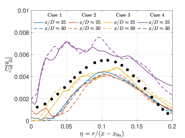
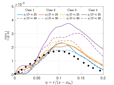
(a)                        (b)

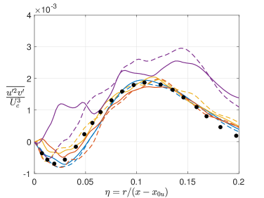
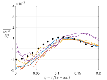
(c)                        (d)

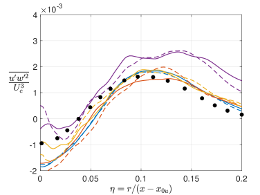
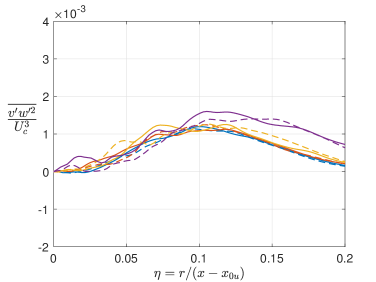
(e)                        (f)

Figure 10: Case 1–4 comparisons: Radial profiles of the normalized third-order velocity moments. (a) $\overline{u^{\prime 3}}/U_{c}^{3}$, (b) $\overline{v^{\prime 3}}/U_{c}^{3}$, (c) $\overline{u^{\prime 2}v^{\prime}}/U_{c}^{3}$, (d) $\overline{u^{\prime}v^{\prime 2}}/U_{c}^{3}$, (e) $\overline{u^{\prime}w^{\prime 2}}/U_{c}^{3}$ and (f) $\overline{v^{\prime}w^{\prime 2}}/U_{c}^{3}$. The black markers $\bullet$ show profiles from the experiments of Panchapakesan & Lumley (1993).

4.1.4 Passive scalar mixing

To assess whether there are mixing differences among Cases 1–4 emulating those of the velocity field, the one-point scalar probability density function (p.d.f.) is examined in figure 11 at various centerline locations. The p.d.f., $\mathcal{P}\left(\xi\right)$, is defined such that

$$\intop_{0}^{1}\mathcal{P}\left(\tilde{\xi}\right)\mathrm{d}\tilde{\xi}=1\qquad\textrm{and}\qquad\bar{\xi}=\intop_{0}^{1}\tilde{\xi}\mathcal{P}\left(\tilde{\xi}\right)\mathrm{d}\tilde{\xi}.$$ (18)

Comparisons between Cases 1 and 2, shown in figure 11(a), evaluate the effect of $p_{\infty}$ increase at approximately same $Z$ value. At $x/D\approx 5$, the centerline contains pure jet fluid $\left(\xi=1\right)$ in both cases. The potential core closes downstream of $x/D\approx 5$, and the p.d.f. at $x/D\approx 8$ in both cases shows a wide spread with mixed-fluid concentration in the range $0.3\lesssim\xi\lesssim 1$. Velocity/pressure statistics in the transition region of Cases 1 and 2 differ significantly, as observed in figures 5, 6 and 8(a). Similarly, $\overline{\xi}$ and $\xi_{\textrm{rms}}^{\prime}$ vary in the transition region yielding differences in mixed-fluid composition and $\mathcal{P}\left(\xi\right)$. In the transition region, the mean scalar concentration decays at a faster rate in Case 1 than in Case 2, as shown in figure 12(a). As a result, downstream of $x/D\approx 10$, the p.d.f. peaks are closer to the jet pure fluid concentration $\left(\xi=1\right)$ in Case 2 than in Case 1, indicating lesser mixing in Case 2 compared to Case 1. For $x/D\geq 10$, the absolute scalar fluctuations $\xi^{\prime}_{c,\textrm{rms}}/\xi_{0}$ are slightly larger in Case 2 than in Case 1, despite smaller normalized local fluctuation $\xi^{\prime}_{c,\textrm{rms}}/\xi_{c}$ in Case 2 between $10\geq x/D\geq 20$, as shown in figure 12(b). Larger $\xi_{c,\textrm{rms}}^{\prime}/\xi_{0}$ implies wider p.d.f. profiles with smaller peaks, indicating larger fluctuations in the mixed-fluid composition and, hence, greater mixing in Case 2 compared to Case 1. However, due to the large jet width downstream of $x/D\approx 15$, the scalar fluctuations at the centerline mix the already (partially) mixed fluid in the vicinity of the centerline and not the pure ambient fluid with the jet fluid. As a result, the p.d.f. peaks showing the mean mixed-fluid concentration continue to be closer to the jet pure fluid concentration $\left(\xi=1\right)$ in Case 2 than in Case 1.

Figure 11(b) compares the scalar p.d.f. from Cases 3 and 4 to examine the effect of $Z$ on mixing behavior at supercritical pressure. Analogous to figure 11(a), the p.d.f. profiles at $x/D\approx 5$ and $8$ are largely similar between the two cases. Differences in peak scalar value, representing the mean concentration, arise in the transition region, consistent with the observations in figure 12. Large scalar fluctuations around $x/D\approx 10$ in Case 4 compared to Case 3 leads to greater mixing in Case 4 in the transition region, resulting in the p.d.f. peaks that are closer to the jet pure fluid concentration $\left(\xi=1\right)$ in Case 3 than in Case 4. At locations downstream of $x/D\approx 15$, the slightly larger $\xi_{c,\textrm{rms}}^{\prime}/\xi_{0}$ in Case 3 compared to Case 4 leads to wider p.d.f. profiles with smaller peaks in Case 3. However, the large jet width downstream of $x/D\approx 15$ causes mixing of the already (partially) mixed fluid in the vicinity of the centerline and, hence, the p.d.f. peaks continue to be closer to the jet pure fluid concentration in Case 3 than in Case 4.

(a)

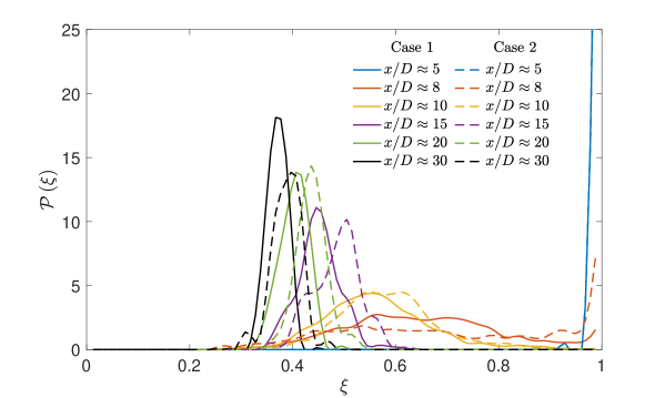
(b)

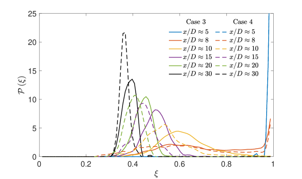
Figure 11: Scalar probability density function, $\mathcal{P}\left(\xi\right)$, at various centerline axial locations for (a) Cases 1 and 2, and (b) Cases 3 and 4.

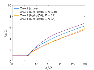
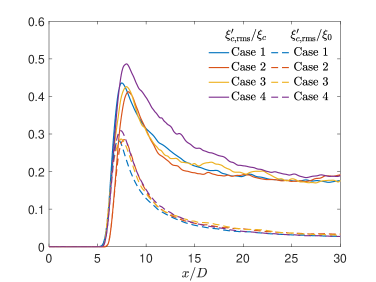
(a)                        (b)

Figure 12: Case 1–4 comparisons: Streamwise variation of the (a) inverse of centerline scalar concentration ($\xi_{c}$) normalized by the jet-exit centerline value ($\xi_{0}$) and (b) centerline r.m.s. scalar fluctuation ($\xi^{\prime}_{c,\textrm{rms}}$) normalized by the centerline mean value, $\xi_{c}$, and jet-exit mean value, $\xi_{0}$.

4.1.5 Summary

The examination of the influence of $p_{\infty}$ and $Z$ on flow statistics in laminar-inflow jets at fixed $Re_{D}$ yields several conclusions. The velocity statistics (mean and fluctuations) attain self-similarity in high-$p$ compressible jets. The flow exhibits sensitivity to $p_{\infty}$ and $Z$ in the transition as well as the self-similar region, with larger differences observed in the transition region. The normalized pressure and density flucutations in the flow follow the behavior of the non-dimensional quantity $p_{\infty}\left(\beta_{T}-1/p_{\infty}\right)$, listed in table 3, that provides a measure other than $Z$ to estimate departure from perfect gas. Proximity of the ambient flow conditions to the Widom line increases $p_{\infty}\left(\beta_{T}-1/p_{\infty}\right)$ and enhances the normalized pressure and density flucutations in the flow, especially in the transition region. The velocity behavior (mean and fluctuations) can be explained in terms of the spatial variation of the normalized pressure-velocity correlations and third-order velocity moments that determine the transport terms in the t.k.e. equation. Increase in velocity fluctuations also enhances the scalar fluctuations, leading to greater centerline mixing in Case 4 compared to the other cases.

4.2 Effects of supercritical pressure at a fixed compressibility factor

The above analysis examined the effects of $Z$ at a fixed supercritical $p_{\infty}$. To examine its counterpart, the influence of $p_{\infty}$ at a fixed $Z$ of $0.9$ is studied here by comparing results between Cases 3 and 5 (see table 2). The value of $p_{\infty}\left(\beta_{T}-1/p_{\infty}\right)$ is slightly larger in Case 3 compared to Case 5, a fact which according to the results of §4.1 should lead to larger local pressure/density fluctuations in Case 3.

The differences in the centerline profiles of the mean axial velocity and mean scalar concentration between Cases 3 and 5, presented in figure 13(a), are minimal in the transition region and they diminish in the self-similar region. Similar to figure 13(a), minor differences are observed in the velocity half-radius ($r_{\frac{1}{2}u}$), shown in figure 13(b), between Cases 3 and 5. In comparison, small but noticeable differences are observed in scalar half-radius ($r_{\frac{1}{2}\xi}$), where the jet spread in Case 3 is slightly larger than that in Case 5.

To further examine the differences between Case 3 and Case 5, a comparison of the normalized centerline velocity, pressure and density fluctuations is shown in figure 14. Centerline r.m.s. axial-velocity fluctuations with two different normalizations are compared in figure 14(a). $U_{0}$ has the same value for Cases 3 and 5, therefore, $u^{\prime}_{c,\textrm{rms}}/U_{0}$ compares the absolute fluctuation magnitude. In contrast, $u^{\prime}_{c,\textrm{rms}}/U_{c}$ depicts the fluctuation magnitude with respect to local mean value. Case 3 exhibits slightly larger $u^{\prime}_{c,\textrm{rms}}/U_{c}$ and $u^{\prime}_{c,\textrm{rms}}/U_{0}$ in the transition region than Case 5, as expected from the slightly greater $U_{c}$ decay in Case 3 than Case 5 in figure 13. The normalized pressure and density fluctuations, illustrated in figure 14(b), show similarly that $p^{\prime}_{c,\textrm{rms}}/p_{c}$ and $\rho^{\prime}_{c,\textrm{rms}}/\rho_{c}$ are larger in Case 3 than Case 5 in the transition region of the flow.

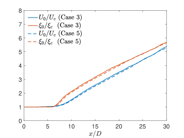
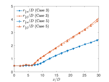
(a)                        (b)

Figure 13: Case 3 and 5 comparisons: Streamwise variation of the (a) inverse of centerline mean axial velocity ($U_{c}$) and scalar ($\xi_{c}$) normalized by the jet-exit centerline values $U_{0}$ and $\xi_{0}$, respectively, and (b) velocity and scalar half radius ($r_{\frac{1}{2}u}$ and $r_{\frac{1}{2}\xi}$).

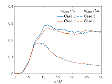
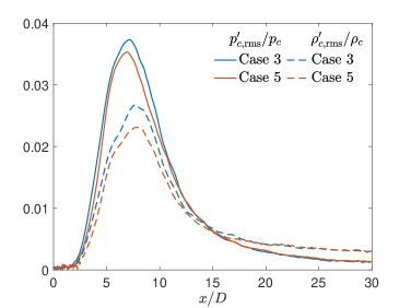
(a)                        (b)

Figure 14: Case 3 and 5 comparisons: Streamwise variation of (a) the centerline r.m.s. axial velocity fluctuations ($u_{c,\mathrm{rms}}^{{}^{\prime}}$) normalized by the centerline mean axial velocity ($U_{c}$) and centerline jet-exit axial velocity ($U_{0}$), and (b) the centerline r.m.s. pressure and density fluctuations, denoted by $p^{\prime}_{c,\mathrm{rms}}$ and $\rho^{\prime}_{c,\mathrm{rms}}$, respectively, normalized by the centerline mean pressure ($p_{c}$) and density ($\rho_{c}$), respectively.

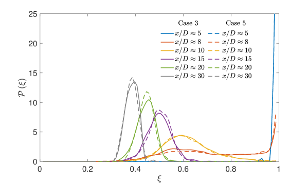
Figure 15: Case 3 and 5 comparisons: Scalar probability density function, $\mathcal{P}\left(\xi\right)$, at various centerline axial locations.

Whether these slightly larger fluctuations in Case 3 lead to greater mixing is assessed using $\mathcal{P}\left(\xi\right)$ in figure 15. While the p.d.f.s at various axial locations look nearly identical, at locations in the transition region and downstream, i.e. $x/D\gtrsim 10$, the p.d.f. peaks are smaller and the profiles somewhat wider in Case 3, a fact which indicates slightly larger scalar fluctuations and greater mixing than in Case 5. This indicates that at same $Z$, larger velocity and thermodynamic fluctuations lead to enhanced mixing.

These results demonstrate that $Z$ does not uniquely determine flow dynamics because Cases 3 and 5 that differ in $p_{\infty}$ but have same $Z$ exhibit small but noticeable differences in flow fluctuations and mixing. In particular, an increase in supercritical $p_{\infty}$ at a fixed $Z$ leads to a reduced normalized velocity/pressure/density/scalar fluctuations, especially in the transition region. Therefore, the possible notion of performing experiments at a fixed $Z$ and inferring from them information to another state having the same $Z$ (i.e. same departure from perfect-gas behavior) but larger $p_{\infty}$, where experiments are more challenging, may be erroneous. Additionally, these results show that $p_{\infty}\left(\beta_{T}-1/p_{\infty}\right)$ may also not be the non-dimensional thermodynamic parameter that completely determines flow behavior, since despite a large change in its value from Case 3 to Case 5 (approximately 30% change), the results of the two cases are relatively close.

In thermodynamics, the law of corresponding states indicates that fluids at the same reduced temperature and reduced pressure have the same $Z$ and, thus, exhibit similar departure from a perfect gas behavior. However, in fluid flows, dynamic effects characterized by the flow Mach number (here $Ma_{e}$) are also important, in addition to the thermodynamic effects characterized by $Z$, in determining the flow behavior. Differences in $Ma_{e}$ arise across Cases 1–5 from the differences in the ambient speed of sound, and the effects of these differences are examined next.

4.3 Effects of $p_{\infty}$ and $Z$ at a fixed jet-exit Mach number

Comparisons between Cases 1–4 in §4.1 evaluated the effects of $p_{\infty}$ and $Z$ at a fixed jet-exit (inflow) bulk velocity, $U_{e}$. Different ambient thermodynamic conditions in Cases 1–4 leads to different ambient speed of sound, $c_{\infty}$, and hence different jet-exit (inflow) Mach number, $Ma_{e}$, values as shown in table 2. Thus, the results discussed so far do not distinguish between the influence of Mach number and the influence of thermodynamic conditions. While a detailed assessment of the effects of Mach number is beyond the scope of this study, some conclusions may be extracted using results from Cases 2M and 4M that have the same ambient thermodynamic conditions as Cases 2 and 4, respectively, but where $U_{e}$ is varied to yield a $Ma_{e}$ of 0.6, which is the same value as that in Case 1. The change in $U_{e}$ from Case 2, where $Ma_{e}=0.58$, to Case 2M is small, but from Case 4, where $Ma_{e}=0.82$, to Case 4M is significant.

The centerline mean axial-velocity, plotted in figure 16(a), shows minor change from Case 2 to 2M but notable differences between Cases 4 and 4M. The small increase in $Ma_{e}$ from Case 2 to Case 2M does not substantially affect the transition region behavior but slightly increases the self-similar axial-velocity decay rate, $1/B_{u}$ in (19), from $1/5.4$ in Case 2 to $1/5.35$ in Case 2M, whereas the decrease in $Ma_{e}$ from Case 4 to Case 4M decreases the mean axial-velocity decay in the transition region as well as in the self-similar region, where $1/B_{u}$ reduces from $1/4.4$ in Case 4 to $1/4.8$ in Case 4M. The velocity half-radius, $r_{\frac{1}{2}u}$, showing the jet spread in figure 16(b) depicts a similar behavior, where minimal differences are observed between Cases 2 and 2M, while the jet spread in Case 4M is considerably reduced with respect to Case 4. This shows that the unique behavior of Case 4, discussed in §4.1, is a combined effect of its proximity to the Widom line and the inflow Mach number. This finding provides the motivation to examine the jet flow sensitivity to inflow condition in §4.4.

To explore the differences observed in figure 16, the normalized velocity and pressure fluctuations among various cases are compared in figure 17. As noted in §4.1.2, the magnitude of $u^{\prime}_{c,\mathrm{rms}}/U_{c}$ reflects the transfer of kinetic energy from the mean field to flucutations and, consequently, its behavior in figure 17(a) is correlated with the mean flow behavior in figure 16(a). Larger $U_{c}$ decay rates in figure 16(a) occur in the regions of larger $u^{\prime}_{c,\mathrm{rms}}/U_{c}$ in figure 17(a). Furthermore, the increase in $Ma_{e}$ from Case 2 to Case 2M enhances $p^{\prime}_{c,\mathrm{rms}}/p_{c}$, as seen in figure 17(b), whereas the decrease in $Ma_{e}$ from Case 4 to Case 4M reduces it. At fixed $Ma_{e}=0.6$, $p^{\prime}_{c,\mathrm{rms}}/p_{c}$ increases with decrease in $Z$ from Case 1 to Case 2M to Case 4M, indicating the role of $Z$ at a fixed $Ma_{e}$. Thus, figure 17(b) in conjunction with figure 8(a) shows that while at a fixed $U_{e}$, the comparative behavior of $p^{\prime}_{c,\mathrm{rms}}/p_{c}$ is correlated with the value of $p_{\infty}\left(\beta_{T}-1/p_{\infty}\right)$ in table 3, this may not be the case at a fixed $Ma_{e}$.

Examination of normalized fluctuating pressure-velocity correlation and third-order velocity moments (not presented here for brevity) showed that their behavior is correlated with the mean and fluctuating axial velocity behavior in figures 16(a) and 17(a), respectively. This feature of the flow is further investigated in the next section to explain the physical mechanism by which thermodynamic and inflow conditions influence jet flow dynamics and mixing.

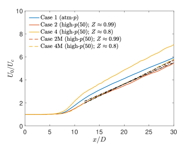
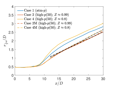
(a)                        (b)

Figure 16: Fixed $U_{e}$ versus fixed $Ma_{e}$ cases: Streamwise variation of (a) the inverse of centerline mean axial velocity ($U_{c}$) normalized by the jet-exit centerline velocity ($U_{0}$) and (b) the velocity half radius ($r_{\frac{1}{2}u}$) normalized by the jet diameter. The black dash-dotted lines in (a) are given by equation (19) using $B_{u}=5.35$, $x_{0u}=0.5D$ for Case 2M, and $B_{u}=4.8$, $x_{0u}=2.5D$ for Cases 4M. The black dash-dotted lines in (b) are given by: $r_{\frac{1}{2}u}/D=0.08\left(x/D+1.6\right)$ for Case 2M, and $r_{\frac{1}{2}u}/D=0.09\left(x/D-0.5\right)$ for Case 4M. The self-similar profiles for Cases 1, 2 and 4 are in figure 5 caption.

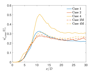
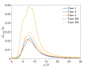
(a)                        (b)

Figure 17: Fixed $U_{e}$ versus fixed $Ma_{e}$ cases: Streamwise variation of (a) the centerline r.m.s. axial velocity fluctuations ($u_{c,\mathrm{rms}}^{{}^{\prime}}$) normalized by the centerline mean axial velocity ($U_{c}$) and (b) the centerline r.m.s. pressure fluctuations ($p^{\prime}_{c,\mathrm{rms}}$) normalized by the centerline mean pressure ($p_{c}$).

4.4 Inflow effects

The influence of inflow conditions on near- and far-field jet flow statistics at atmospheric conditions has been a subject of numerous investigations, e.g. Husain & Hussain (1979), Richards & Pitts (1993), Boersma et al. (1998), Mi et al. (2001), Xu & Antonia (2002). Several studies have questioned the classical self-similarity hypothesis Townsend (1980) that the asymptotic state of the jet flow depends only on the rate at which momentum is added and is independent of the inflow conditions. Those studies support the analytical result of George (1989), who suggested that the flow can asymptote to different self-similar states determined by the inflow condition. It is thus pertinent to use the two inflow conditions described in §3.2.2 to examine the uniqueness of the self-similar state at near-atmospheric $p_{\infty}$. In contrast to past investigations in which measurements were obtained of either the velocity or the passive scalar field, here the inflow effects on the velocity and the scalar field are simultaneously examined, first at perfect-gas conditions in 4.4.1, and then at high-$p$ conditions in 4.4.2.

4.4.1 Inflow effects at perfect-gas condition: comparisons between Cases 1 and 1T

For the laminar inflow, which has a top-hat jet-exit mean velocity profile (12), the jet-exit bulk velocity is approximately $U_{e}$, and $U_{e}$ is equal to the jet-exit centerline velocity, $U_{0}$. However, for the turbulent inflow, which has a parabolic jet-exit mean velocity profile, the jet-exit bulk velocity, $U_{e}$, is smaller than $U_{0}$. The present study uses the same $U_{e}$ for all cases, except Cases 2M and 4M. As a result, $U_{0}$ is different for the laminar and turbulent inflow cases.

Figure 18 illustrates the near-field scalar contours from Cases 1 and 1T at $tU_{e}/D\approx 3500$. The rendered contour lines show the mixed fluid, defined as $0.02\leq\xi\leq 0.98$. Evidently, the near-field flow features are considerably different for the two jets. The instabilities in the annular shear layer that trigger vortex roll-ups appear at larger axial distance in the jet from the laminar inflow (Case 1) than those in the jet from the pseudo-turbulent inflow (Case 1T). The inflow disturbances in Case 1T, modeling pipe-flow turbulence, are broadband and higher in magnitude, thus triggering small-scale turbulence that promote axial shear-layer growth immediately downstream of the jet exit. In contrast, the laminar inflow has small random disturbances superimposed over the top-hat velocity profile that trigger the natural instability frequency Ho & Nosseir (1981) and dominant vortical structures/roll-up around $x/D\approx 5$. The larger axial distance required for the natural instability to take effect in Case 1 leads to a longer potential core than in Case 1T. However, once the instabilities take effect in Case 1, at $x/D\approx 5$, dominant vortical structures close the potential core over a short distance, i.e. around $x/D\approx 8$. In comparison, in Case 1T, the broadband small-scale turbulence triggered immediately downstream of the jet exit closes the potential core around $x/D\approx 6$. Downstream of the potential core collapse, an abrupt increase in the jet width is observed in Case 1, while the jet grows gradually in Case 1T.

(a)

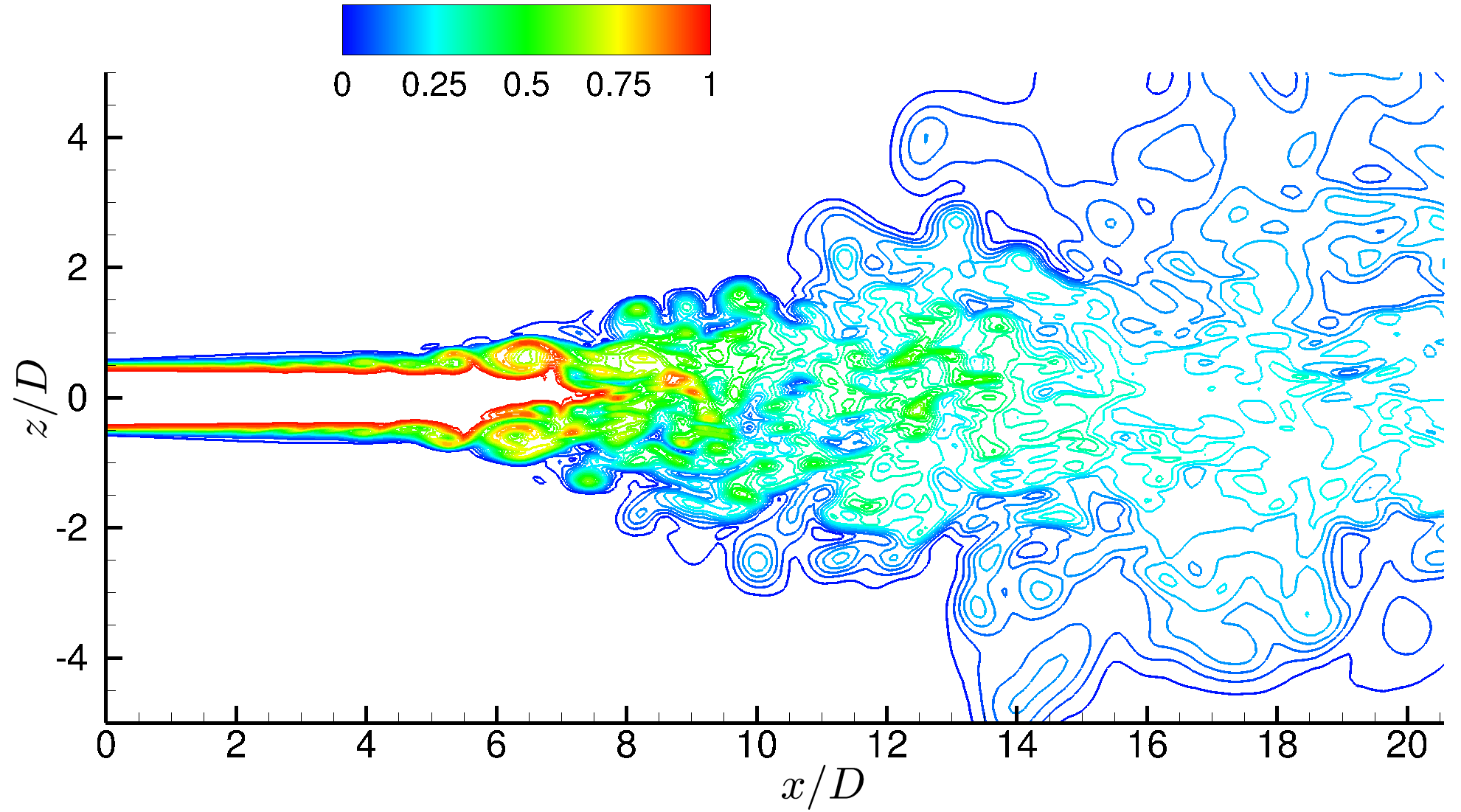
(b)

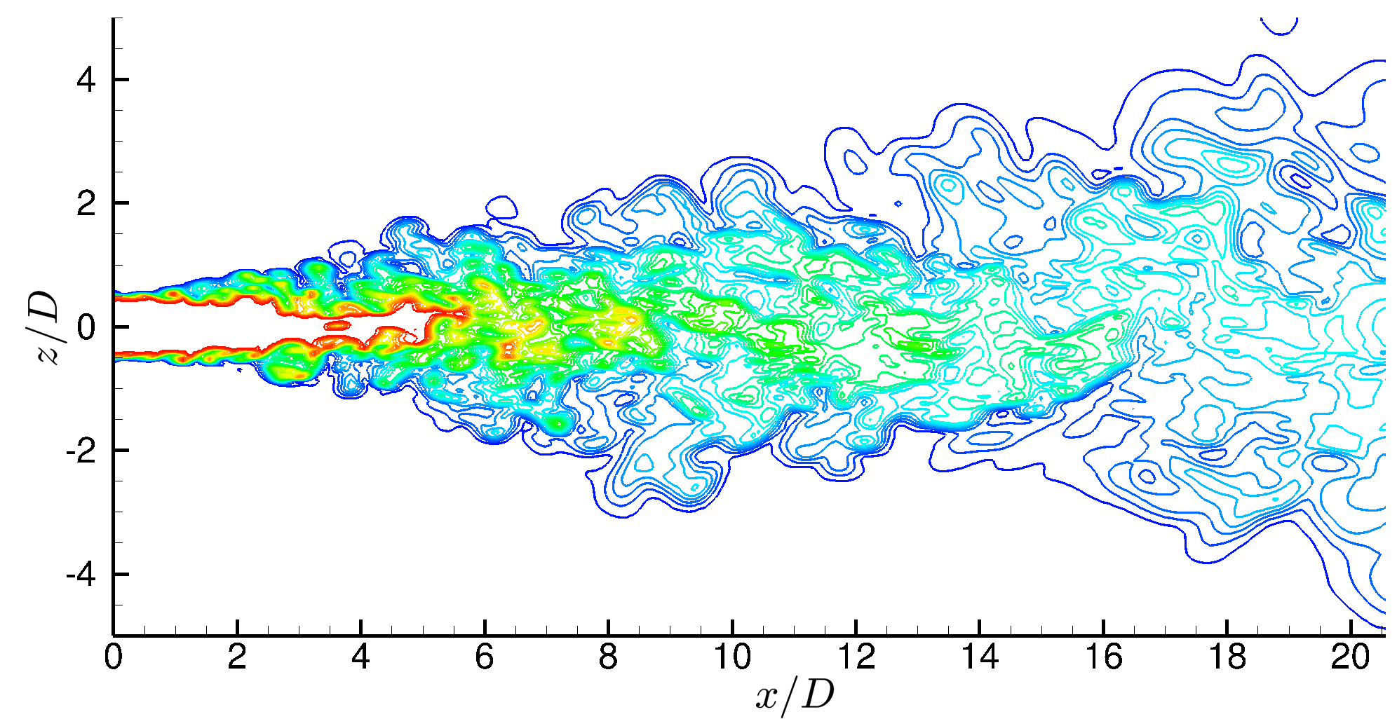
Figure 18: Near-field instantaneous scalar contours at $tU_{e}/D\approx 3500$ from (a) Case 1 and (b) Case 1T showing the mixed fluid concentration. The contour lines show 24 levels in the range $0.02\leq\xi\leq 0.98$. The legend is the same for both plots.

The above-discussed qualitative differences are now quantified using various velocity and scalar statistics.

4.4.1.1   Velocity and scalar statistics, and self-similarity

A comparison of $U_{c}$ and $\xi_{c}$ axial decay between Case 1 and Case 1T jets is presented in figure 19(a). The shorter potential core length of Case 1T leads to velocity and scalar decay beginning upstream of that in Case 1. The difference between the axial locations where the velocity and scalar begin to decay is noticeable for Case 1, while it is relatively small for Case 1T thus indicating a tighter coupling of dynamics and molecular mixing in Case 1T. The upstream decay of the scalar, with respect to velocity, in the laminar inflow jet (Case 1) is consistent with the observation of (Lubbers et al., 2001, Figure 6) for a passive scalar diffusing at unity Schmidt number. Also noticeable in the Case 1 results is a transition or development region, $7\lesssim x/D\lesssim 15$, where the velocity and scalar decay rates are larger than in the asymptotic state reached further downstream. The Case 1T results do not show a similarly distinctive transition region, and the velocity and scalar decay rates remain approximately the same downstream of the potential core closure. Downstream of $x/D\approx 15$, the velocity and scalar decay rates are similar for Cases 1 and 1T.

The velocity and scalar half-radius for Cases 1 and 1T are compared in figure 19(b). The Case 1 jet spreads at a faster rate than Case 1T, consistent with the experimental observations of Xu & Antonia (2002) and Mi et al. (2001). The decrease in velocity half-radius spreading rate from $0.085$ (Case 1) to $0.078$ (Case 1T) is consistent with the observations of Xu & Antonia (2002), where a decrease in spreading rate from $0.095$ for the jet issuing from a smooth contraction nozzle to $0.086$ for the jet from a pipe nozzle was reported. The spreading rate of $0.14$ and $0.11$ based on the scalar half-radius for Case 1 and Case 1T, respectively, is larger than the values of $0.11$ and $0.102$ reported by Mi et al. (2001) for their temperature scalar field from smooth contraction nozzle and pipe jet, respectively, but comparable to the values of $0.13$ and $0.11$ deduced from the results of Richards & Pitts (1993) for their mass-fraction scalar field from smooth contraction nozzle and pipe jet, respectively. The profiles in figure 19 also show that the velocity and scalar mean fields attain self-similarity, i.e. their centerline values decay linearly and the half-radius spreads linearly, at smaller axial distance in Case 1T than in Case 1. In the self-similar region, the $U_{c}$ and $\xi_{c}$ decay rates of Cases 1 and 1T are comparable, while the half-radius spreading rates differ. The non-dimensional $U_{0}/U_{c}$ have similar values for Cases 1 and 1T in the self-similar region, but since $U_{0}$ is different for Case 1 and Case 1T, $U_{c}$ differs accordingly. The results of mean velocity/scalar centerline behavior and jet spread suggest that these quantities strongly depend on the inflow condition, both in the near-field and the self-similar region, thus highlighting the importance of reporting inflow conditions in experimental studies if their data has to be used for model validation.

To further examine the differences between Cases 1 and 1T, and the self-similar state attained in these flows, the radial variation of axial velocity and its fluctuation is documented in figure 20. Examination of figure 20(a) shows that the mean axial velocity attains self-similarity as near-stream as $x/D\approx 15$ for both Case 1 and 1T, however, the self-similar profiles are different. The solid markers in figure 20(a) show the $f\left(\eta\right)$ profiles of (17) using $A_{u}=79.5$ (circles) and $99$ (triangles). These values are comparable to the values of $76.5$ and $90.2$ reported by Xu & Antonia (2002) for jets from a smooth contraction and pipe nozzle, respectively. Radial profiles of $u^{\prime}_{\textrm{rms}}/U_{c}$ from Cases 1 and 1T are compared in figure 20(b). $u^{\prime}_{\textrm{rms}}/U_{c}$ attains self-similarity around $x/D\approx 25$, a location which is further downstream than for $\overline{u}/U_{c}$, in both Cases 1 and 1T; minor differences remain near the centerline between the profiles at $x/D\approx 25$ and $30$. $u^{\prime}_{\textrm{rms}}/U_{c}$ values from Case 1T are smaller than those from Case 1 at all shown axial locations, especially away from the centerline, consistent with the experimental observations of Xu & Antonia (2002) with laminar/turbulent inflow. Figure 20(b) also shows that for Case 1, $u^{\prime}_{\textrm{rms}}/U_{c}$ in the near field ($x/D\approx 15$) is larger than that in the self-similar regime, especially in the radial vicinity of the centerline, while for Case 1T, the near field ($x/D\approx 15$) values are smaller than that in the self-similar regime. $u^{\prime}_{\textrm{rms}}/U_{c}$ values in the near field are, therefore, considerably larger with laminar inflow than with turbulent inflow. The behavior of other Reynolds stress components, $v^{\prime}_{\textrm{rms}}/U_{c}$, $w^{\prime}_{\textrm{rms}}/U_{c}$, and $\overline{u^{{}^{\prime}}v^{{}^{\prime}}}/U_{c}^{2}$, not shown here for brevity, is similar to that of $u^{\prime}_{\textrm{rms}}/U_{c}$ in that all of them show self-similarity around $x/D\approx 25$ but the self-similar profiles depend on the inflow condition. Moreover, their near field values are much higher in Case 1 than in Case 1T, as for $u^{\prime}_{\textrm{rms}}/U_{c}$. Thus, similar to the mean quantities in figure 19, the Reynolds stress components also show strong sensitivity to the inflow condition.

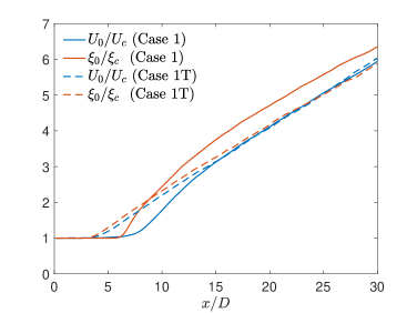
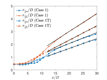
(a)                        (b)

Figure 19: Case 1 and 1T comparisons: Streamwise variation of the (a) inverse of centerline mean axial-velocity ($U_{c}$) and scalar concentration ($\xi_{c}$) normalized by the jet-exit centerline mean values and (b) normalized velocity and scalar half radius, denoted by $r_{\frac{1}{2}u}/D$ and $r_{\frac{1}{2}\xi}/D$, respectively. The linear profile downstream of $x/D\approx 15$ in (a) can be described by equation (19) using $B_{u}=5.5$ ($x_{0u}=-2.4D$) and $B_{\xi}=5.75$ ($x_{0\xi}=-3.5D$) for Case 1T, whereas $B_{u}=5.5$ ($x_{0u}=-2.4D$) and $B_{\xi}=5.7$ ($x_{0\xi}=-6.8D$) for Case 1. The black solid lines in (b) are given by: $r_{\frac{1}{2}u}/D=0.085\left(x/D+4.4\right)$ and $r_{\frac{1}{2}\xi}/D=0.14\left(x/D+1.5\right)$ for Case 1, and $r_{\frac{1}{2}u}/D=0.078\left(x/D+1.7\right)$ and $r_{\frac{1}{2}\xi}/D=0.11\left(x/D+0.85\right)$ for Case 1T.

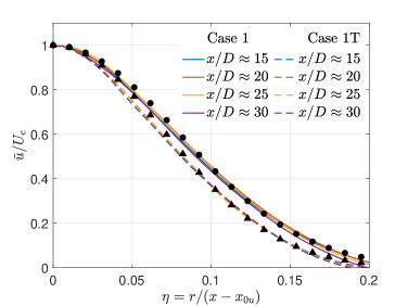
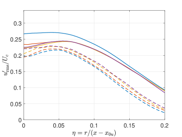
(a)                        (b)

Figure 20: Case 1 and 1T comparisons: Radial profiles of (a) mean axial velocity ($\bar{u}$) and (b) r.m.s. axial velocity fluctuations ($u_{\mathrm{rms}}^{{}^{\prime}}$) normalized by the centerline mean velocity ($U_{c}$) at various axial locations. The markers $\bullet$ and $\blacktriangle$ in (a) show $f\left(\eta\right)$ of equation (17) using $A_{u}=79.5$ and $99$, respectively. The legend is the same for both plots.

4.4.1.2   Passive scalar mixing

To examine the differences in scalar mixing between Cases 1 and 1T, figure 21 compares the scalar p.d.f., $\mathcal{P}\left(\xi\right)$, at various locations along the jet centerline. Significant differences are observed in the near-field p.d.f. profiles, i.e. for $x/D\lesssim 15$. The locations $x/D\approx 5$ and $8$ are approximately the centerline location of maximum (non-dimensionalized) scalar fluctuations for Case 1T and Case 1, respectively, as shown in figure 22. Since the jet-exit centerline mean scalar value is $\xi_{0}=1$ for all cases, normalization of $\xi^{\prime}_{c,\textrm{rms}}$ with $\xi_{0}$ in figure 22 allows a comparison of the absolute fluctuation magnitude between Case 1 and Case 1T. $\xi^{\prime}_{c,\textrm{rms}}/\xi_{0}$ peaks when the potential core closes and, then, decreases with axial distance for each case. In contrast, the local normalization with $\xi_{c}$ asymptotes to a constant value at large axial distances. $\xi^{\prime}_{c,\textrm{rms}}/\xi_{c}$ exhibits a prominent hump, or a local maximum, in the near field for Case 1, consistent with the experimental observations in jets from a smooth contraction nozzle Mi et al. (2001).

Comparison of p.d.f. profiles at $x/D\approx 5$ in figure 21 between Case 1 and 1T shows pure jet fluid ($\xi=1$) for Case 1, whereas mixed fluid with scalar concentrations ranging from $0.5$ to $1$ for Case 1T, as expected, since the potential core closes before $x/D\approx 5$ in Case 1T, but after $x/D\approx 5$ in Case 1. At $x/D\approx 8$ and $10$, the p.d.f. profiles for Case 1 exhibit a wider spread compared to that for Case 1T. Stronger large-scale vortical structures in the near field (around $x/D\approx 8$) in Case 1, as seen in figure 18(a), entrain ambient fluid deep into the jet core resulting in larger scalar fluctuations (see figure 22) and a wider distribution of scalar concentrations at the centerline. In contrast, mixing in Case 1T occurs through small-scale structures resulting in weaker entrainment of ambient fluid and smaller scalar fluctuations. P.d.f. profiles for Case 1T at $x/D\approx 8$ and $10$ are, therefore, narrower with higher peaks. Larger scalar fluctuations in the transition region ($7\lesssim x/D\lesssim 15$) of Case 1, resulting from large-scale organized structures, cause greater mixing and, consequently, steeper decay of the centerline mean scalar concentration $\left(\xi_{c}\right)$, as observed in figure 19(a). The centerline mean scalar concentration, indicated by the scalar value at peaks of the p.d.f. profiles in figure 21, is smaller (or closer to the ambient scalar value of $0$) for Case 1 downstream of $x/D\approx 10$. The difference between the scalar mean values from the two cases diminishes with axial distance. With increase in axial distance, the jet-width (see figure 19(b)) increases and the absolute centerline scalar fluctuation (see figure 22) diminishes. As a result, the spread of the scalar p.d.f. profile declines and the peaks become sharper downstream of $x/D\approx 10$.

4.4.1.3   Summary

To conclude, both velocity and scalar statistics show sensitivity to the inflow condition. In the near field, the jet flow from laminar inflow (Case 1) is characterized by strong vortical structures leading to larger velocity/scalar fluctuations and jet spreading rate in the transition region than Case 1T. Further downstream, self-similarity is observed in velocity/scalar mean and fluctuations, but the self-similar profiles differ with the inflow, supporting the argument that they may not be universal. This indicates that a quantitative knowledge of the experimental inflow conditions is important in validating simulation results against experiments. Whether these conclusions hold at high pressures is examined next.

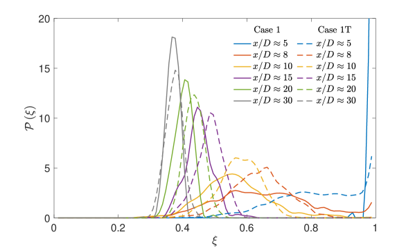
Figure 21: Case 1 and 1T comparisons: Scalar probability density function, $\mathcal{P}\left(\xi\right)$, at various centerline axial locations.

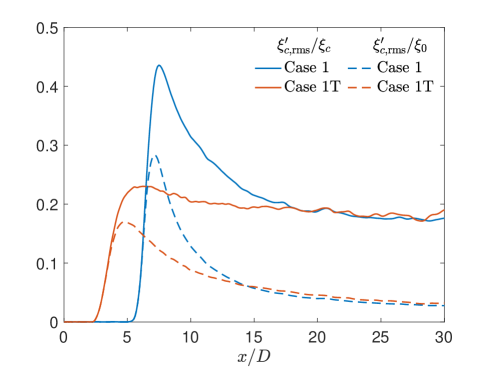
Figure 22: Case 1 and 1T comparisons: Streamwise variation of the centerline r.m.s. scalar fluctuation ($\xi^{\prime}_{c,\textrm{rms}}$) normalized by the centerline mean scalar value ($\xi_{c}$) and the jet-exit centerline mean scalar value ($\xi_{0}$).

4.4.2 Inflow effects at high pressure: comparisons between Cases 1/1T, 2/2T and 4/4T

A crucial observation from §4.1, where the influence of $p_{\infty}$ and $Z$ on jet-flow dynamics and mixing was examined, is that $p^{\prime}_{c,\textrm{rms}}/p_{c}$ decreases with increase in $p_{\infty}$ from $1$ bar (Case 1) to $50$ bar (Case 2), and increases with decrease in $Z$ from $0.99$ (Case 2) to $0.8$ (Case 4), as shown in figure 8(a); the velocity/scalar mean and fluctuations (figures 5(a), 6 and 12), however, follow the behavior of the normalized t.k.e. diffusive fluxes (and not of $p^{\prime}_{c,\textrm{rms}}/p_{c}$), e.g. $\frac{\overline{p^{\prime}u^{\prime}}/\bar{\rho}}{U_{c}^{3}}$ and $\overline{u^{\prime 3}}/U_{c}^{3}$ shown in figures 8(b) and (c), respectively. Those observations are for laminar inflow jets, and the validity of those observations is here examined in pseudo-turbulent inflow jets (inflow details in §3.2.2).

To examine the effects of inflow variation at supercritical $p_{\infty}$, Case 2 results are here compared with Case 2T, and Case 4 with Case 4T. These results in conjunction with those of §4.4.1 provide an enlarged understanding of the effect of inflow conditions at different $p_{\infty}$ and $Z$.

4.4.2.1   Mean axial velocity and spreading rate

Figure 23(a) illustrates the centerline variation of mean axial velocity in Cases 1/1T, 2/2T and 4/4T. In concurrence with the observation for Case 1T against Case 1, discussed in §4.4.1, the pseudo-turbulent inflow cases at supercritical pressure (Cases 2T and 4T) also exhibit a shorter potential core than their laminar inflow counterparts (Cases 2 and 4). As a result, the axial location where the mean velocity decay begins for Cases 1T, 2T and 4T is upstream of the corresponding location for Cases 1, 2 and 4. The laminar inflow cases show a distinct transition region ($7\lesssim x/D\lesssim 15$) with larger mean velocity decay rate than that further downstream in their self-similar region. A similar change in decay rate (equal to the slope of the plot lines) does not occur in Cases 1T, 2T and 4T, where the slopes remain approximately the same downstream of the potential core closure. The linear decay rate in the self-similar region is described by $1/B_{u}$, defined by equation (19). The $B_{u}$ values for various cases are included in the caption of figure 23(a). For Cases 1 and 1T, the decay rates are the same; between Cases 2 and 2T, the decay rate is slightly larger in the laminar inflow jet (Case 2), and between Cases 4 and 4T, the decay rate is significantly larger in the laminar inflow jet (Case 4).

To investigate the differences in jet spread, $r_{\frac{1}{2}u}$ from different inflow cases are compared in figure 23(b). As expected from smaller potential core length in the pseudo-turbulent inflow cases, $r_{\frac{1}{2}u}$ growth in Cases 1T, 2T and 4T begins upstream of that in Cases 1, 2 and 4. Immediately downstream of the potential core closure, $r_{\frac{1}{2}u}$ in laminar inflow cases (Cases 1, 2 and 4) grows at a relatively faster rate than in Cases 1T, 2T and 4T. The linear $r_{\frac{1}{2}u}$ profiles in the self-similar region of Cases 1, 2, 4 and 1T are given in figures 5 and 19. The profiles for Cases 2T and 4T are listed in the figure caption. The inflow change from laminar to pseudo-turbulent reduces the spreading rate at atmospheric as well as supercritical conditions. The change is significant at atmospheric conditions (from $0.085$ in Case 1 to $0.078$ in Case 1T) and relatively small for supercritical cases (from $0.0805$ in Case 2 to $0.079$ in Case 2T and $0.077$ in Case 4 to $0.076$ in Case 4T). A noticeable feature in the self-similar region of figure 23(b) is the difference in $r_{\frac{1}{2}u}$ among various cases for the two inflows; for laminar inflow, $r_{\frac{1}{2}u}$ decreases from Case 1 to Case 2 and increases from Case 2 to Case 4, whereas the differences are comparatively minimal between Cases 1T, 2T and 4T. In fact, $r_{\frac{1}{2}u}$ in Cases 1T and 2T are slightly larger than that in Case 4T.

The decay in mean velocity occurs in part due to the transfer of kinetic energy from the mean field to fluctuations, as discussed in §4.1.1. To determine if the differences observed here in the mean velocity are consistent with the variations in velocity fluctuations, they are examined next.

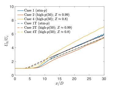
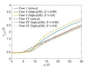
(a)                        (b)

Figure 23: Comparisons of different inflow cases: Streamwise variation of the (a) inverse of centerline mean velocity ($U_{c}$) normalized by the jet-exit centerline velocity ($U_{0}$) and (b) velocity half-radius ($r_{\frac{1}{2}u}$). The black dash-dotted lines in (a) are given by equation (19) using $B_{u}=5.5$, $x_{0u}=-2.3D$ for Case 2T and $B_{u}=5.7$, $x_{0u}=-1.3D$ for Case 4T. Details of lines showing the self-similar profile of equation (19) for Cases 1, 2, 4 and 1T are presented in figures 5 and 19. The black dotted lines in (b) are given by $r_{\frac{1}{2}u}/D=0.079\left(x/D+2.2\right)$ for Case 2T and $r_{\frac{1}{2}u}/D=0.076\left(x/D+1.3\right)$ for Case 4T.

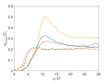
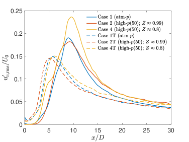
(a)                        (b)

Figure 24: Comparisons of different inflow cases: Streamwise variation of the (a) the centerline r.m.s. axial velocity fluctuations ($u_{c,\mathrm{rms}}^{{}^{\prime}}$) normalized by the centerline mean axial velocity ($U_{c}$), (b) $u_{c,\mathrm{rms}}^{{}^{\prime}}$ normalized by the jet-exit centerline mean axial velocity ($U_{0}$). The legend is the same for both plots.

4.4.2.2   Velocity fluctuations and self-similarity

To understand the differences observed in figure 23, the centerline variation of axial-velocity fluctuations is compared for various inflow cases in figure 24. $u_{c,\textrm{rms}}^{\prime}/U_{c}$, presented in figure 24(a), reflects the local mean energy transfer to fluctuations. As discussed in §4.1, higher $u^{\prime}_{c,\textrm{rms}}/U_{c}$ implies larger mean axial-velocity decay rate or higher slope of the line in figure 23(a). In the transition region, the laminar inflow cases exhibit significant differences with increase in $p_{\infty}$ (from Case 1 to Case 2) as well as with decrease in $Z$ (from Case 2 to Case 4). In contrast, the differences are minimal between Cases 1T, 2T and 4T. In the transition region of these cases $\left(3\lesssim x/D\lesssim 8\right)$, $u^{\prime}_{c,\textrm{rms}}/U_{c}$ in Case 4T is slightly smaller than that in Cases 1T and 2T. Accordingly, the mean axial-velocity decay rate is smaller for Case 4T in the transition region, see figure 23(a). The difference between the asymptotic value attained by $u^{\prime}_{c,\textrm{rms}}/U_{c}$ is small between Cases 1 and 1T, but significant at supercritical $p_{\infty}$ between Cases 2 and 2T and Cases 4 and 4T. The difference is particularly large between Cases 4 and 4T, consistent with the large difference in their $U_{c}$ decay rates in the self-similar region of figure 23. Thus, the variation in axial-velocity fluctuations consistently represents the transfer of mean kinetic energy to t.k.e.

Normalizing $u^{\prime}_{c,\textrm{rms}}$ with $U_{0}$, as presented in figure 24(b), enables a comparison of the absolute fluctuation magnitude for each inflow ($U_{0}$ differs for the two inflows, as discussed in §4.4.1). In figure 24(b), $u^{\prime}_{c,\textrm{rms}}/U_{0}$ decreases with axial distance, unlike $u^{\prime}_{c,\textrm{rms}}/U_{c}$ in figure 24(a) that asymptotes to a constant value. The peak of $u^{\prime}_{c,\textrm{rms}}/U_{0}$, attained in the transition region, decreases with increasing $p_{\infty}$ from $1$ bar to $50$ bar and increases with decreasing $Z$ from $0.99$ to $0.8$ for each inflow. The $u^{\prime}_{c,\textrm{rms}}/U_{c}$ and $u^{\prime}_{c,\textrm{rms}}/U_{0}$ magnitudes and their differences are larger in the laminar inflow cases, especially in the transition region of the flow, showing that the effect of $p_{\infty}$ and $Z$ depends strongly on the inflow, in addition to the ambient thermodynamic state characterized by $p_{\infty}\left(\beta_{T}-1/p_{\infty}\right)$.

To examine self-similarity in the flow, the radial variations of mean axial velocity and r.m.s. axial-velocity flucutations at three axial locations are compared between Cases 2 and 2T and Cases 4 and 4T in figures 25 and 26, respectively. The axial location $x/D\approx 10$ lies around the jet transition region in both inflow cases, whereas the profiles at $x/D\approx 25$ and $30$ help assess self-similarity. Figure 25(a) shows that $\bar{u}/U_{c}$ attains self-similarity upstream of $x/D\approx 25$ in both cases (2 and 2T); however, the self-similar profile is different as shown by the least-squares fits of the Gaussian distribution, $f\left(\eta\right)$ of (17), to $x/D\approx 30$ profiles, depicted as solid black markers in figure 25(a). $u^{\prime}_{\textrm{rms}}/U_{c}$ profiles at $x/D\approx 25$ and $30$ in figure 25(b) exhibit only minor differences in both Cases 2 and 2T, suggesting that $u^{\prime}_{\textrm{rms}}/U_{c}$ is self-similar around $x/D\approx 25$. $u^{\prime}_{\textrm{rms}}/U_{c}$ is considerably larger in the laminar inflow case (Case 2) at all $\eta$ locations, consistent with the observations at atmospheric $p_{\infty}$ between Cases 1 and 1T in figure 20(b). Similarly, $v^{\prime}_{\textrm{rms}}/U_{c}$, $w^{\prime}_{\textrm{rms}}/U_{c}$, and $\overline{u^{\prime}v^{\prime}}/U{}_{c}^{2}$ (not shown here for brevity) are also larger in Case 2 than Case 2T and show self-similarity around $x/D\approx 25$.

$\bar{u}/U_{c}$ from Cases 4 and 4T are compared in figure 26(a). As in figures 20(a) and 25(a) for Cases 1/1T and 2/2T, the self-similar profile are different for the two inflows, and this difference is amplified with respect to Cases 2/2T as the solid markers in figure 26(a) that display the Gaussian distribution, $f\left(\eta\right)$ of (17), show. $u^{\prime}_{\textrm{rms}}/U_{c}$ illustrated in figure 26(b) shows self-similarity around $x/D\approx 25$ for both cases (4 and 4T) and larger magnitude in the laminar inflow case (Case 4). $v^{\prime}_{\textrm{rms}}/U_{c}$, $w^{\prime}_{\textrm{rms}}/U_{c}$, and $\overline{u^{\prime}v^{\prime}}/U{}_{c}^{2}$ show similar behavior, and are not shown here for brevity.

The spatial variation of thermodynamic (pressure/density) fluctuations and their correlation with velocity fluctuations that determines the transport terms in the t.k.e. equation were used to explain the jet flow dynamics for various $p_{\infty}$ and $Z$ in §4.1.3 and, therefore, these quantities are examined next to determine if they can explain the differences with inflow condition discussed above.

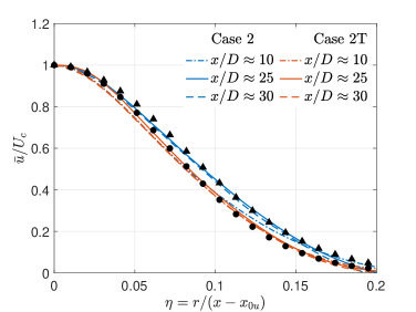
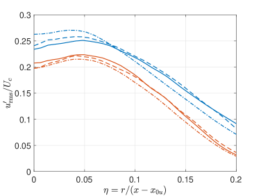
(a)                        (b)

Figure 25: Case 2 and 2T comparisons:Radial profiles of (a) mean axial velocity ($\bar{u}$) normalized by the centerline mean axial velocity ($U_{c}$), (b) r.m.s. axial-velocity fluctuations ($u^{\prime}_{\mathrm{rms}}$) normalized by the centerline mean axial velocity at various axial locations. The markers $\blacktriangle$ and $\bullet$ in (a) show $f\left(\eta\right)$ of equation (17) using $A_{u}=79.5$ and $99.2$, respectively. The legend is the same for both plots.

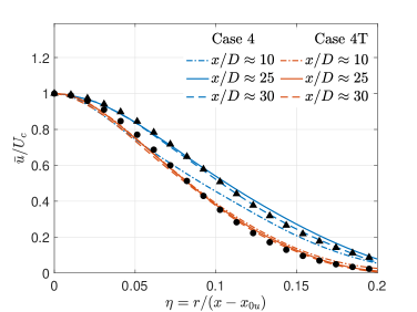
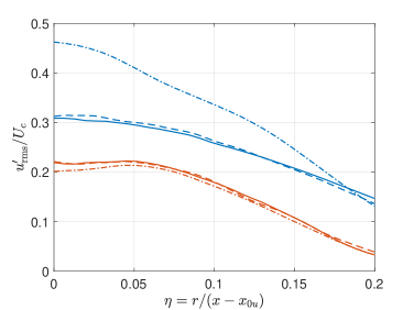
(a)                        (b)

Figure 26: Case 4 and 4T comparisons:Radial profiles of (a) mean axial velocity ($\bar{u}$) normalized by the centerline mean axial velocity ($U_{c}$), (b) r.m.s. axial-velocity fluctuations ($u^{\prime}_{\mathrm{rms}}$) normalized by the centerline mean axial-velocity at various axial locations. The markers $\blacktriangle$ and $\bullet$ in (a) show $f\left(\eta\right)$ of equation (17) using $A_{u}=64.4$ and $99.2$, respectively. The legend is the same for all plots.

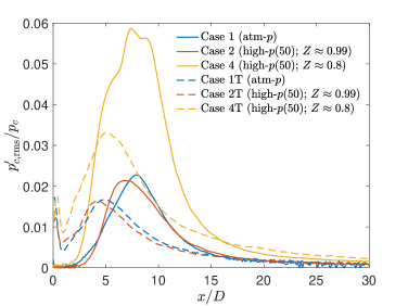
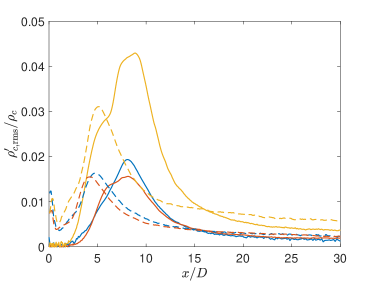
(a)                        (b)

Figure 27: Comparisons of different inflow cases: Streamwise variation of the (a) the centerline r.m.s. pressure ($p^{\prime}_{c,\mathrm{rms}}$) normalized by the centerline mean pressure ($p_{c}$) and (b) the centerline r.m.s. density fluctuations ($\rho^{\prime}_{c,\mathrm{rms}}$) normalized by the centerline mean density ($\rho_{c}$). The legend is the same for both plots.

4.4.2.3   Pressure and density fluctuations, pressure-velocity correlation, and third-order velocity moments

Centerline variations of $p_{c,\text{rms}}^{\prime}/p_{c}$ and $\rho_{c,\text{rms}}^{\prime}/\rho_{c}$ are presented in figures 27(a) and (b), respectively. $p^{\prime}_{c,\textrm{rms}}/p_{c}$ and $\rho^{\prime}_{c,\textrm{rms}}/\rho_{c}$ are negligible at jet exit in laminar inflow cases but have significant magnitude in pseudo-turbulent inflow cases, where it decreases with axial distance until the potential core closes and increases in the transition region. Variations of $p^{\prime}_{c,\textrm{rms}}/p_{c}$ and $\rho^{\prime}_{c,\textrm{rms}}/\rho_{c}$ with $p_{\infty}$ and $Z$ are similar for the two inflows. $p^{\prime}_{c,\textrm{rms}}/p_{c}$ and $\rho^{\prime}_{c,\textrm{rms}}/\rho_{c}$ are larger in Case 4 than in Cases 1 and 2 and, similarly, they are higher in Case 4T than in Cases 1T and 2T. With increase in $p_{\infty}$ from 1 bar (Cases 1 and 1T) to 50 bar (Cases 2 and 2T), the peak value of $p^{\prime}_{c,\textrm{rms}}/p_{c}$ and $\rho^{\prime}_{c,\textrm{rms}}/\rho_{c}$ in the transition region decreases by a small value. The differences diminish downstream in the self-similar region. $p^{\prime}_{c,\textrm{rms}}/p_{c}$ and $\rho^{\prime}_{c,\textrm{rms}}/\rho_{c}$ increase with decrease in $Z$ from $0.99$ (Cases 2 and 2T) to $0.8$ (Cases 4 and 4T) for both inflows, especially in the transition region of the flow. On the other hand, $u^{\prime}_{c,\textrm{rms}}/U_{c}$, presented in figure 24(a), increases with decreasing $Z$ for laminar inflow but remains approximately the same in pseudo-turbulent inflow cases. In fact, in the transition region, $u^{\prime}_{c,\textrm{rms}}/U_{c}$ is slightly smaller in Case 4T than Case 2T, while it is larger in Case 4 than Case 2. This anomaly with inflow change leads to contrasting mean flow behavior, observed in figure 23 in the transition region, where the mean axial-velocity decay and jet half-radius increases from Case 2 to Case 4 but decreases from Case 2T to Case 4T.

To investigate this anomaly, the centerline variation of t.k.e. diffusion fluxes from turbulent transport is compared in figures 28 and 29. Figure 28 compares $\frac{\overline{p^{\prime}u^{\prime}}/\bar{\rho}}{U_{c}^{3}}$, which determines the t.k.e. diffusion due to pressure fluctuation transport. To highlight the differences among pseudo-turbulent inflow cases with suitable $y$-axis scale, figure 28(b) shows only the results from Cases 1T, 2T and 4T. In the transition region, the absolute magnitude of $\frac{\overline{p^{\prime}u^{\prime}}/\bar{\rho}}{U_{c}^{3}}$ increases from Case 2 to Case 4 but decreases from Case 2T to 4T, indicating that the t.k.e. diffusion due to pressure fluctuation transport increases in the laminar inflow jet but decreases in the pseudo-turbulent inflow jet. Further downstream, the differences are significant between Cases 2 and 4, but minimal between Cases 2T and 4T, implying that the effects of $Z$ (or the effects of ambient thermodynamic conditions closer to the Widom line) are enhanced in the laminar inflow jets.

$\overline{u^{\prime 3}}/U_{c}^{3}$, which determines t.k.e. diffusion flux from turbulent transport of $\overline{u^{\prime 2}}$, is compared between Cases 1/1T, 2/2T and 4/4T in figure 29(a) and among cases 1T/2T/4T in figure 29(b). While there are significant differences in $\overline{u^{\prime 3}}/U_{c}^{3}$ profiles of Cases 1, 2 and 4, the differences are, again, minimal among Cases 1T, 2T and 4T. Thus, both $\frac{\overline{p^{\prime}u^{\prime}}/\bar{\rho}}{U_{c}^{3}}$ and $\overline{u^{\prime 3}}/U_{c}^{3}$ show greater sensitivity to the ambient thermodynamic state, characterized by $p_{\infty}\left(\beta_{T}-1/p_{\infty}\right)$, in the laminar inflow jets, and their variation in figures 28 and 29 for various cases agrees well with the behavior of $u^{\prime}_{c,\textrm{rms}}/U_{c}$ in figure 24(a) and the mean-flow metrics in figure 23.

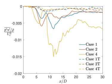
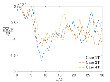
(a)                        (b)

Figure 28: Comparisons of different inflow cases: Streamwise variation of the normalized pressure-axial velocity correlation for (a) the laminar and pseudo-turbulent inflow cases, and (b) only the pseudo-turbulent inflow cases. Note the difference between $y$-axis scales of (a) and (b).

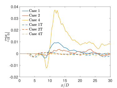
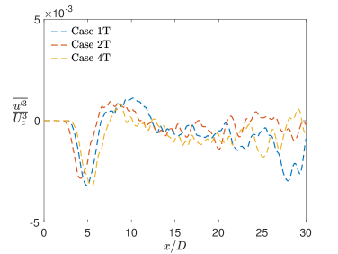
(a)                        (b)

Figure 29: Comparisons of different inflow cases: Streamwise variation of $\overline{u^{\prime 3}}/U_{c}^{3}$ for (a) the laminar and pseudo-turbulent inflow cases, and (b) only the pseudo-turbulent inflow cases. Note the difference between $y$-axis scales of (a) and (b).

4.4.2.4   Passive scalar mixing

To examine passive scalar mixing with inflow change at high pressure, the scalar p.d.f. is depicted in figure 30; Cases 2 and 2T are compared at various $x/D$ in figure 30(a) and, similarly, Cases 4 and 4T are compared in figure 30(b). As observed at atmospheric $p_{\infty}$ (figure 21), the p.d.f. at $x/D\approx 5$ in figure 30(a) shows pure jet fluid in the laminar inflow case (Case 2), whereas mixed fluid in the case of pseudo-turbulent inflow (Case 2T). At $x/D\approx 8$ and $10$, the p.d.f. has a wider distribution in Case 2 owing to stronger large-scale vortical structures that yield larger normalized scalar fluctuations, $\xi^{\prime}_{c,\textrm{rms}}/\xi_{0}$, as shown in figure 31(b). Further downstream, the p.d.f. profiles show minor differences, consistent with the scalar mean and fluctuation behavior observed in figure 31. Thus, at supercritical $p_{\infty}$, but with ambient conditions far from the Widom line (with near-unity $Z$), the influence of the inflow on scalar mixing is restricted to near field. Figure 30(b) shows that the situation changes when the ambient conditions are closer to the Widom line. Although the differences in $\mathcal{P}\left(\xi\right)$ at $x/D\approx 5$ and $8$, influenced by the potential core length, are similar to those in figures 21 and 30(a), significant differences are observed between the downstream $\mathcal{P}\left(\xi\right)$ profiles (at $x/D\approx 15$, 20 and $30$) of Case 4/4T in figure 30(b), unlike Cases 2/2T. For Case 4, the $\mathcal{P}\left(\xi\right)$ peaks are further away from the jet pure fluid concentration ($\xi=1$) and are higher than in Case 4T. The peaks in a symmetric unimodal p.d.f. coincide with the mean value, therefore, the differences in p.d.f. peak location and magnitude in figure 30(b) mirrors the differences observed in mean scalar values between Case 4 and Case 4T in figure 31(a).

(a)

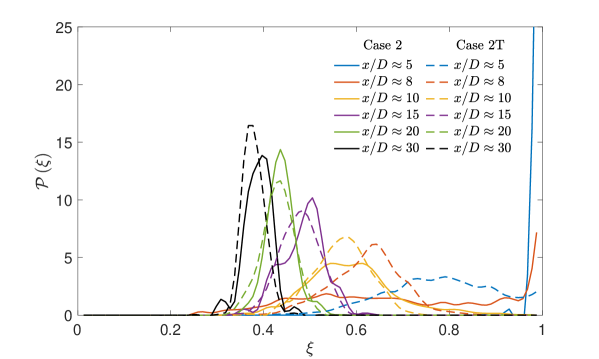
(b)

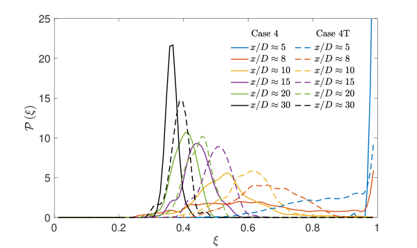
Figure 30: Scalar probability density function, $\mathcal{P}\left(\xi\right)$, at various centerline axial locations for (a) Cases 2 and 2T, and (b) Cases 4 and 4T.

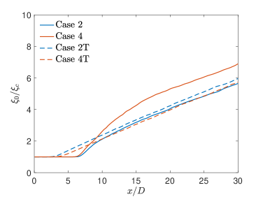
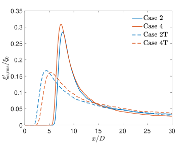
(a)                        (b)

Figure 31: Streamwise variation of the (a) inverse of centerline scalar concentration ($\xi_{c}$) normalized by the jet-exit centerline value ($\xi_{0}$) and (b) centerline r.m.s. scalar fluctuation ($\xi^{\prime}_{c,\textrm{rms}}$) normalized by the centerline jet-exit mean value ($\xi_{0}$).

4.4.2.5   Summary

To summarize the above results, the variation of $p^{\prime}_{c,\textrm{rms}}/p_{c}$ and $\rho^{\prime}_{c,\textrm{rms}}/\rho_{c}$ with $p_{\infty}$ and $Z$ is similar for both inflows (containing different perturbations but same $U_{e}$), as shown in figures 27(a) and (b), and the variation can be estimated from the relative values of $p_{\infty}\left(\beta_{T}-1/p_{\infty}\right)$ for various cases. However, $u^{\prime}_{c,\textrm{rms}}/U_{c}$ shown in figure 24(a) varies differently for the two inflows. With decrease in $Z$, the proximity to the Widom line increases $u^{\prime}_{c,\textrm{rms}}/U_{c}$ in the laminar inflow jet, whereas the same decrease in $Z$ has minimal influence on $u^{\prime}_{c,\textrm{rms}}/U_{c}$ in pseudo-turbulent inflow jet. This suggests that the real-gas effects, quantified by $p_{\infty}\left(\beta_{T}-1/p_{\infty}\right)$, are strongly felt in the laminar inflow jets that contain large-scale coherent structures which generate regions of high mean strain rates, as shown in figure 32(a), whereas the same real-gas effects minimally influence pseudo-turbulent inflow jets. These results also showed that the effects of thermodynamic compressibility on jet flow dynamics cannot be directly determined from the variation of pressure fluctuations, instead fluctuating pressure-velocity correlation and third-order velocity moments (that determine t.k.e. diffusion fluxes from turbulent transport) are better correlated with the behavior of the velocity field.

Studies of dynamic compressibility (e.g. Freund et al., 2000) divide compressibility modeling efforts into explicit and implicit approaches. An explicit approach targets modeling of the dilatational terms in the t.k.e. equation with the assumption that the turbulence characteristics are largely influenced by the compressible terms. In contrast, the implicit approaches assume that compressibility influences the structure of the turbulence, which in turn changes the turbulence energetics reflected in the t.k.e. production and turbulence transport terms. In this study, the behavior of the t.k.e. production term, plotted in figure 32(b), and the turbulence transport terms, discussed above, follow the behavior of $u^{\prime}_{c,\textrm{rms}}/U_{c}$, which suggests that implicit modeling may be the physically correct approach for modeling of thermodynamic compressibility effects.

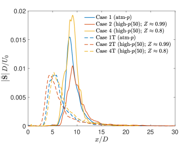
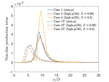
(a)                        (b)

Figure 32: Centerline variation of (a) the strain rate magnitude, $\left|\bar{\mathbf{S}}\right|=\left(2\bar{S}_{ij}\bar{S}_{ij}\right)^{1/2}$, normalized by $U_{0}/D$, where $\bar{S}_{ij}$ is the mean rate-of-strain tensor, and (b) t.k.e. production term $P=-\bar{\rho}\widetilde{u^{\prime\prime}_{i}u^{\prime\prime}_{j}}\frac{\partial\tilde{u}_{i}}{\partial x_{j}}$ normalized by $\rho_{e}$ (jet-exit density), $U_{0}$ and $D$, where tilde $\left(\tilde{\bullet}\right)$ denotes the Favre average, $\tilde{\phi}=\overline{\rho\phi}/\bar{\rho}$, and $u^{\prime\prime}_{i}=u_{i}-\tilde{u}_{i}$.

5 Conclusions

Turbulent round-jet DNS at perfect gas (subcritical) and real gas (supercritical) conditions were performed to compare and contrast the effects of thermodynamic and inflow condition on flow development and passive mixing. In all cases, the Reynolds number, $Re_{D}$, is $5000$. The equation of state and transport coefficient models were chosen to accurately represent the flow conditions. For supercritical pressures, the transport coefficient models were validated with the NIST database. The thermodynamic conditions are characterized in terms of the ambient fluid compressibility factor, $Z$, and normalized isothermal compressibility, $p_{\infty}\left(\beta_{T}-1/p_{\infty}\right)$. The inflow conditions are characterized in terms of the jet-exit bulk velocity ($U_{e}$) or Mach number ($Ma_{e}$) and the perturbation type, namely, a laminar inflow (with top-hat velocity profile and small random perturbations) or a pseudo-turbulent inflow (with statistics matching pipe-flow turbulence).

The first finding is that the mean axial velocity and Reynolds stress components attain self-similarity in high-$p$ fully-compressible jets, as they do in atmospheric-$p$ jets. However, the self-similar profiles depend on the thermodynamic and inflow details, indicating that these details influence both the near- and far-field jet flow dynamics. The transition region of the flow, immediately downstream of the potential core closure, exhibits greater sensitivity to those details than the self-similar region. Moreover, the laminar inflow jets show larger differences with change in thermodynamic conditions than the pseudo-turbulent inflow jets. The laminar inflow jets exhibit dominant coherent structures that generate a transition region with large mean strain rates, which enhance sensitivity to real-gas effects. These coherent structures also enhance the jet spread in laminar inflow cases compared to pseudo-turbulent inflow cases, where the jet spreads by entrainment through small-scale turbulence.

The second important finding is that the ambient thermodynamic conditions influence flow behavior by modifying the structure of turbulence through production and transport of the turbulent kinetic energy (t.k.e.). In jets with a fixed $U_{e}$ and inflow perturbation, the normalized pressure/density fluctuations vary according to the value of $p_{\infty}\left(\beta_{T}-1/p_{\infty}\right)$. Increasing $p_{\infty}\left(\beta_{T}-1/p_{\infty}\right)$ enhances the normalized pressure/density fluctuations in both the laminar inflow and the pseudo-turbulent inflow jets. However, the effect on velocity/scalar fluctuations depends on the extent of thermodynamic departure from perfect gas as well as the inflow perturbations. Large deviation of $Z$ from unity and of $p_{\infty}\left(\beta_{T}-1/p_{\infty}\right)$ from zero with laminar inflow triggers large normalized velocity/scalar fluctuations resulting in greater mixing. However, a small departure from perfect gas does not change the flow behavior significantly. Moreover, the effect of thermodynamic changes on velocity/scalar statistics in pseudo-turbulent inflow jets is small, despite significant variations in their pressure/density statistics. Velocity/scalar fluctuations that determine flow entrainment and mixing are not directly correlated with pressure fluctuations, but rather with the fluctuating pressure-velocity correlation that determines the turbulent transport in the t.k.e. equation due to pressure fluctuations. These results show that the thermodynamic condition, expressed in terms of $Z$ or $p_{\infty}\left(\beta_{T}-1/p_{\infty}\right)$, is insufficient to completely determine the flow behavior that also depends on the inflow details. Thus, neither $Z$ nor $p_{\infty}\left(\beta_{T}-1/p_{\infty}\right)$ are self-similarity parameters.

The third important finding is that at large departures from perfect gas, $U_{e}$ (from which the Mach number $Ma_{e}$ is calculated that determines the dynamic compressibility) can strongly influence flow dynamics and mixing. The ambient speed of sound differs according to the thermodynamic condition and, hence, a fixed $U_{e}$ leads to different $Ma_{e}$ across various flow cases. Variation of $Ma_{e}$ over a small subsonic range shows that an increase in $Ma_{e}$ with laminar inflow enhances velocity/scalar fluctuations leading to greater mixing. Variation of thermodynamic condition at a fixed $Ma_{e}$ shows that the pressure/density fluctuations differ according to the value of $Z$; smaller $Z$ leads to larger fluctuations. The velocity/scalar flucutations in high-$p$ cases also vary according to the $Z$ value. A detailed study of the effects of $Ma_{e}$ is beyond the scope of this study and will be a subject of future investigation.

The jet-flow regions and metrics sensitive to $p_{\infty}$, $Z$ and inflow condition, identified in this study, may guide high-$p$ experimental studies in obtaining measurements that may serve as databases for simulation and model validation. For example, the transition region of laminar-inflow jets exhibits high sensitivity to $Z$, and thus high-resolution measurements in that region may help in evaluating high-$p$ model robustness and accuracy. The results from this study also demonstrate that high-$p$ jet experiments performed at a fixed $Z$ cannot be used to infer results for jets at same $Z$ but larger $p_{\infty}$. Moreover, the larger velocity/scalar fluctuations when the Widom line is approached in laminar inflow jets suggest that fuel-oxidizer mixing can be enhanced by combustor thermodynamic conditions closer to the Widom line with laminar fuel injection. Similarly, the correlation between the normalized pressure/density fluctuations and $p_{\infty}\left(\beta_{T}-1/p_{\infty}\right)$ could be used to predict the thermodynamic fluctuations in a flow at real-gas thermodynamic conditions, without performing the flow simulations.

Appendix A Validation of the EOS and transport properties for high-$p$ simulations

To examine the robustness of the PR EOS and transport coefficient models at supercritical conditions, figure 33 illustrates the density, isobaric heat capacity, and the transport coefficients $\mu_{\mathrm{ph}}$ and $\lambda_{\mathrm{ph}}$ calculated from the models described in §2.3. The calculated values are compared against the National Institute of Standards and Technology (NIST) database Lemmon et al. (2010) for $\mathrm{N_{2}}$ at $p=50$ and $70$ bar in the $T$ range 100 K - 400 K, which includes the critical temperature $T_{cr}=$126.2 K of N₂. As evident, the models have good agreement with the NIST database, showing their validity at high-$p$ conditions. The transport coefficient models are accurate only for $T>T_{cr}$ and, thus, the comparison of $\mu_{\mathrm{ph}}$ and $\lambda_{\mathrm{ph}}$ only spans this range.

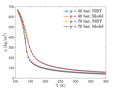
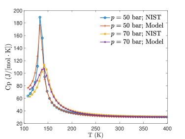
(a)                    (b)

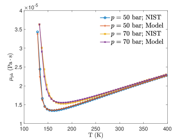
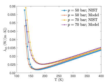
(c)                    (d)

Figure 33: EOS and transport coefficients model comparison against NIST database for pure Nitrogen at $50$ bar pressure. (a) Density, (b) Isobaric heat capacity, (c) Viscosity, and (d) Thermal conductivity.

Appendix B Grid convergence

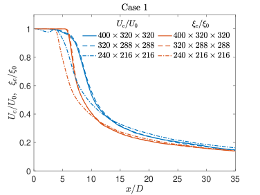
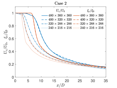
(a)                        (b)

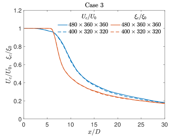
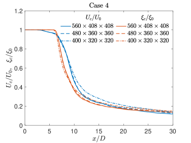
(c)                        (d)

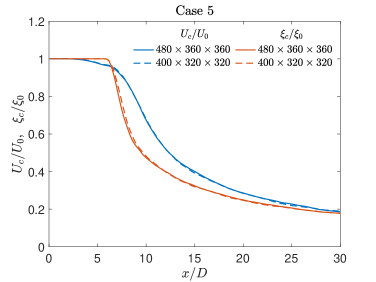
(e)

Figure 34: Time-averaged centerline velocity ($U_{c}$) and scalar ($\xi_{c}$) values normalized by the jet exit values $U_{0}$ and $\xi_{0}$ as a function of axial distance for various grid resolutions. (a) Case 1, (b) Case 2, (c) Case 3, (d) Case 4, and (e) Case 5.

An estimate of the Kolmogorov length scale in terms of $Re_{D}$, which may help determine the optimal grid spacing for DNS, can be made for incompressible (or weakly compressible) jet flows Sharan & Bellan (2019). However, the estimates for incompressible flows may not necessarily apply in high-pressure regimes of interest here. Therefore, to ensure grid convergence, mean flow statistics are compared in this section by successively refining the grid for Cases 1 to 5 (see table 2), which ensures sufficient grid resolution for DNS.

Figures 34(a) to (e) compare the time-averaged centerline velocity, $U_{c}$, and scalar concentration, $\xi_{c}$, normalized by the jet exit values $U_{0}$ and $\xi_{0}$ as a function of axial distance from simulations of Cases 1 to 5 with various grid resolutions. Statistics for Case 1 at atmospheric conditions converges at a resolution of $320\times 288\times 288$, whereas, for high-pressure cases, they converge around $400\times 320\times 320$, except Case 4 at $Z=0.8$ having maximum deviation from perfect gas among all cases considered that shows convergence around $480\times 360\times 360$. The plots also show that in all cases the scalar concentration begins to decay upstream of the velocity and at a faster rate than the velocity, consistent with the observation of (Lubbers et al., 2001, see Figure 6) for a passive scalar diffusing at unity Schmidt number.

Appendix C Validation of perfect-gas simulation: Case 1 results

Quantitative experimental data for supercritical jets are rare, however, numerous measurements of high-order statistics have been made for jets at atmospheric conditions. For comparisons, the experimental measurements made in the self-similar region of density-matched jets, where the jet/chamber density ratio is approximately unity, are considered here, e.g. the velocity measurements of Wygnanski & Fiedler (1969), Panchapakesan & Lumley (1993) and Hussein et al. (1994), and the passive scalar measurements of Ebrahimi & Kleine (1977), Dowling & Dimotakis (1990) and Mi et al. (2001).

Figure 35 shows the decay of the time-averaged centerline velocity, $U_{c}(x)$, and centerline scalar concentration, $\xi_{c}(x)$, normalized by the jet-exit centerline velocity, $U_{0}$ $\left(=U_{c}(0)\right)$, and scalar concentration, $\xi_{0}$ $\left(=\xi_{c}(0)\right)$, respectively, for Case 1. In the self-similar region, $U_{c}$ varies with the reciprocal of the downstream distance, given by (e.g. Hussein et al., 1994)

$$\frac{U_{c}\left(x\right)}{U_{0}}=B_{u}\left(\frac{D}{x-x_{0u}}\right),$$ (19)

where $B_{u}$ is a constant and $x_{0u}$ denotes the virtual origin derived from the centerline axial velocity. Similarly, the time-averaged centerline scalar concentration has the form

$$\frac{\xi_{c}\left(x\right)}{\xi_{0}}=B_{\xi}\left(\frac{D}{x-x_{0\xi}}\right),$$ (20)

where $B_{\xi}$ is a constant and $x_{0\xi}$ denotes the virtual origin derived from the centerline scalar variation. Simultaneous measurements of the velocity and scalar field in a single experiment were not found in literature and, therefore, data from different studies are used for comparing the velocity and scalar fields. The dashed and dash-dotted lines in figure 35(b) show the profiles for $B_{u}=5.5$ and $B_{\xi}=5.7$, respectively. They are comparable to the experimentally observed values of $B_{u}=5.7$, $6.06$ and $5.8$ by Wygnanski & Fiedler (1969), Panchapakesan & Lumley (1993) and Hussein et al. (1994), respectively, and of $B_{\xi}=5.78$ and $5.11$ by Ebrahimi & Kleine (1977) and Dowling & Dimotakis (1990), respectively.

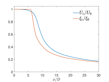
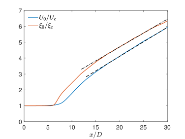
(a)                        (b)

Figure 35: Case 1 results: Streamwise variation of the (a) centerline mean velocity ($U_{c}$) and scalar concentration ($\xi_{c}$) normalized by the respective jet-exit centerline mean values, $U_{0}$ and $\xi_{0}$, as a function of axial distance and (b) inverse of the normalized time-averaged centerline values showing linear decay asymptotically with axial distance. The dashed line uses $B_{u}=5.5$, $x_{0u}=-2.4D$ in (19) and the dash-dotted line uses $B_{\xi}=5.7$, $x_{0\xi}=-6.8D$ in (20).

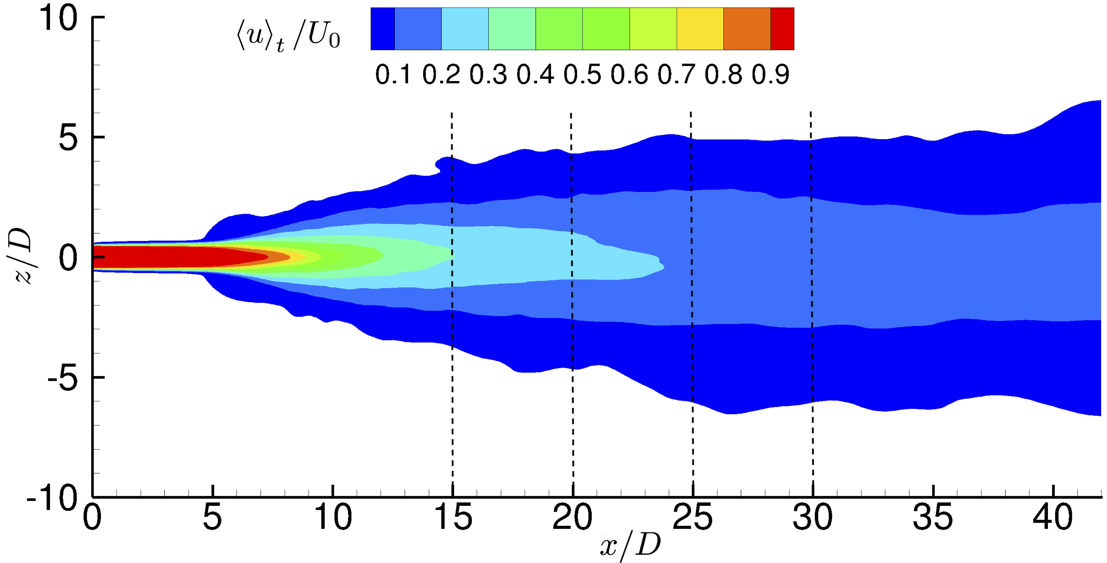
Figure 36: Time-averaged axial velocity contours for Case 1. The dashed lines show axial locations where statistics are azimuthally averaged.

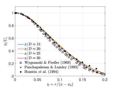
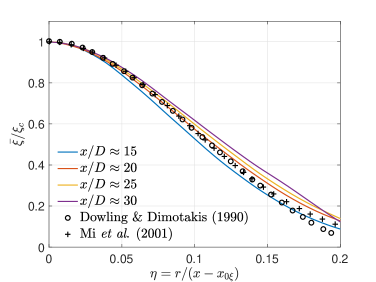
(a)                      (b)

Figure 37: Case 1 results: (a) Mean axial velocity ($\bar{u}$) normalized by the centerline mean velocity ($U_{c}$) and (b) mean scalar concentration ($\bar{\xi}$) normalized by the centerline mean scalar value at various axial locations plotted as a function of similarity coordinates. The velocity profiles are compared against the self-similar profiles from the experiments of Wygnanski & Fiedler (1969), Panchapakesan & Lumley (1993) and Hussein et al. (1994), whereas the scalar profiles are compared against the experimental profiles of Dowling & Dimotakis (1990) and Mi et al. (2001).

Contours of $\left\langle u\right\rangle_{t}/U_{0}$ in the $y/D=0$ plane are depicted in figure 36, with dashed lines showing the axial locations where $\bar{u}/U_{c}$ and $\bar{\xi}/\xi_{c}$ are plotted in figure 37(a) and (b), respectively. The azimuthal averages for calculations of $\bar{u}$ and $\bar{\xi}$ using (14) are performed by interpolation of the time-averaged Cartesian-grid solution to a polar grid at respective axial locations. The variation of $\bar{u}/U_{c}$ with the similarity coordinate, $\eta=r/\left(x-x_{0u}\right)$, is compared with the self-similar profile from experiments in figure 37(a). The simulation results at various axial locations agree well with each other and with the experimental profiles, indicating that the mean axial velocity becomes self-similar around $x/D\approx 15$ for this case. $\bar{\xi}/\xi_{c}$ at various $x/D$ locations is compared against the self-similar profiles of Dowling & Dimotakis (1990) and Mi et al. (2001) in figure 37(b). As evident from the figure, there are minor differences between the profiles at various axial locations, suggesting that the mean scalar concentration is not fully self-similar, but close to self-similarity around $x/D\approx 30$.

To further examine the velocity field, figure 38(a) and (b) show the radial variation of normalized root-mean-square (r.m.s.) axial-velocity fluctuation and Reynolds stress compared against the self-similar profile from experiments. The simulation profiles at $x/D\approx 25$ and $x/D\approx 30$, in figure 38, agree well with each other, indicating that these quantities attain self-similarity downstream of $x/D\approx 20$. The simulation self-similar profiles also lie within the experimentally observed self-similar profiles of these quantities.

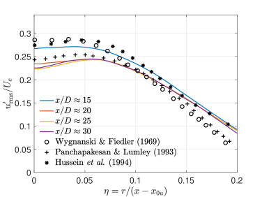
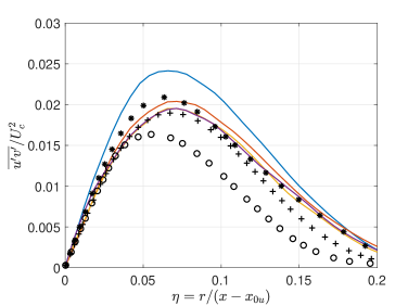
(a)                        (b)

Figure 38: Case 1 results: (a) r.m.s. axial velocity fluctuations ($u_{\mathrm{rms}}^{{}^{\prime}}$), and (b) Reynolds stress ($\overline{u^{{}^{\prime}}v^{{}^{\prime}}}$) normalized by the centerline mean velocity at various axial locations plotted as a function of similarity coordinates compared against the self-similar profiles from the experiments of Wygnanski & Fiedler (1969), Panchapakesan & Lumley (1993) and Hussein et al. (1994). The legend is the same for both plots.

The favorable comparisons between simulation results and experimental measurements indicate that the governing equations with perturbed laminar inflow and the numerical method accurately simulate the jet exiting a smooth contracting nozzle at atmospheric-$p$. More comparisons are not included here for brevity, but can be found in Sharan & Bellan (2021).

References

- Baab et al. (2016) Baab, S., Förster, F. J., Lamanna, G. & Weigand, B. 2016 Speed of sound measurements and mixing characterization of underexpanded fuel jets with supercritical reservoir condition using laser-induced thermal acoustics. Experiments in Fluids 57 (11), 172.
- Baab et al. (2018) Baab, S., Steinhausen, C., Lamanna, G., Weigand, B. & Förster, F. J. 2018 A quantitative speed of sound database for multi-component jet mixing at high pressure. Fuel 233, 918–925.
- Balaras et al. (2001) Balaras, E., Piomelli, U. & Wallace, J. M. 2001 Self-similar states in turbulent mixing layers. Journal of Fluid Mechanics 446, 1.
- Banuti et al. (2017) Banuti, D. T., Raju, M. & Ihme, M. 2017 Similarity law for widom lines and coexistence lines. Physical Review E 95 (5), 052120.
- Bodony (2006) Bodony, D. J. 2006 Analysis of sponge zones for computational fluid mechanics. Journal of Computational Physics 212 (2), 681–702.
- Boersma et al. (1998) Boersma, B. J., Brethouwer, G. & Nieuwstadt, F. 1998 A numerical investigation on the effect of the inflow conditions on the self-similar region of a round jet. Physics of Fluids 10 (4), 899–909.
- Chehroudi et al. (2002) Chehroudi, B., Talley, D. & Coy, E. 2002 Visual characteristics and initial growth rates of round cryogenic jets at subcritical and supercritical pressures. Physics of Fluids 14 (2), 850–861.
- Dowling & Dimotakis (1990) Dowling, D. R. & Dimotakis, P. E. 1990 Similarity of the concentration field of gas-phase turbulent jets. Journal of Fluid Mechanics 218, 109–141.
- Ebrahimi & Kleine (1977) Ebrahimi, I. & Kleine, R. 1977 Konzentrationsfelder in isothermen luft-freistrahlen. Forschung im Ingenieurwesen A 43 (1), 25–30.
- Eggels et al. (1994) Eggels, J., Unger, F., Weiss, M. H., Westerweel, J., Adrian, R. J., Friedrich, R. & Nieuwstadt, F. 1994 Fully developed turbulent pipe flow: a comparison between direct numerical simulation and experiment. Journal of Fluid Mechanics 268, 175–210.
- Falgout et al. (2015) Falgout, Z., Rahm, M., Wang, Z. & Linne, M. 2015 Evidence for supercritical mixing layers in the ECN Spray A. Proceedings of the Combustion Institute 35 (2), 1579–1586.
- Freund et al. (2000) Freund, J. B., Lele, S. K. & Moin, P. 2000 Compressibility effects in a turbulent annular mixing layer. Part 1. Turbulence and growth rate. Journal of Fluid Mechanics 421, 229–267.
- Gao et al. (2019) Gao, W., Lin, Y., Hui, X., Zhang, C. & Xu, Q. 2019 Injection characteristics of near critical and supercritical kerosene into quiescent atmospheric environment. Fuel 235, 775–781.
- George (1989) George, W. K. 1989 The self-preservation of turbulent flows and its relation to initial conditions and coherent structures. Advances in Turbulence 3973.
- George & Davidson (2004) George, W. K. & Davidson, L. 2004 Role of initial conditions in establishing asymptotic flow behavior. AIAA Journal 42 (3), 438–446.
- Ghosal & Rogers (1997) Ghosal, S. & Rogers, M. M. 1997 A numerical study of self-similarity in a turbulent plane wake using large-eddy simulation. Physics of Fluids 9 (6), 1729–1739.
- Gnanaskandan & Bellan (2017) Gnanaskandan, A. & Bellan, J. 2017 Numerical simulation of jet injection and species mixing under high-pressure conditions. J. Phys 821, 012020.
- Gnanaskandan & Bellan (2018) Gnanaskandan, A. & Bellan, J. 2018 Side-jet effects in high-pressure turbulent flows: Direct numerical simulation of nitrogen injected into carbon dioxide. The Journal of Supercritical Fluids 140, 165–181.
- Grinstein (2001) Grinstein, F. F. 2001 Vortex dynamics and entrainment in rectangular free jets. Journal of Fluid Mechanics 437, 69–101.
- Harstad et al. (1997) Harstad, K. G., Miller, R. S. & Bellan, J. 1997 Efficient high-pressure state equations. AIChE Journal 43 (6), 1605–1610.
- Ho & Nosseir (1981) Ho, C. M. & Nosseir, N. S. 1981 Dynamics of an impinging jet. part 1. the feedback phenomenon. Journal of Fluid Mechanics 105, 119–142.
- Husain & Hussain (1979) Husain, Z. D. & Hussain, A. K. M. F. 1979 Axisymmetric mixing layer: influence of the initial and boundary conditions. AIAA Journal 17 (1), 48–55.
- Hussein et al. (1994) Hussein, H. J., Capp, S. P. & George, W. K. 1994 Velocity measurements in a high-reynolds-number, momentum-conserving, axisymmetric, turbulent jet. Journal of Fluid Mechanics 258, 31–75.
- Kennedy & Carpenter (1994) Kennedy, C. A. & Carpenter, M. H. 1994 Several new numerical methods for compressible shear-layer simulations. Applied Numerical Mathematics 14 (4), 397–433.
- Klein et al. (2003) Klein, M., Sadiki, A. & Janicka, J. 2003 A digital filter based generation of inflow data for spatially developing direct numerical or large eddy simulations. Journal of Computational Physics 186 (2), 652–665.
- Lele (1994) Lele, S. K. 1994 Compressibility effects on turbulence. Annual Review of Fluid Mechanics 26 (1), 211–254.
- Lemmon et al. (2010) Lemmon, E. W., Huber, M. L., McLinden, M. O. & others 2010 NIST standard reference database 23. NIST Reference Fluid Thermodynamic and Transport Properties—REFPROP, Version 9, 55.
- Lodato et al. (2008) Lodato, G., Domingo, P. & Vervisch, L. 2008 Three-dimensional boundary conditions for direct and large-eddy simulation of compressible viscous flows. Journal of Computational Physics 227 (10), 5105–5143.
- Lubbers et al. (2001) Lubbers, C. L., Brethouwer, G. & Boersma, B. J. 2001 Simulation of the mixing of a passive scalar in a round turbulent jet. Fluid Dynamics Research 28 (3), 189.
- Lund et al. (1998) Lund, T. S., Wu, X. & Squires, K. D. 1998 Generation of turbulent inflow data for spatially-developing boundary layer simulations. Journal of Computational Physics 140 (2), 233–258.
- Masi et al. (2013) Masi, E., Bellan, J., Harstad, K. G. & Okong’o, N. A 2013 Multi-species turbulent mixing under supercritical-pressure conditions: modelling, direct numerical simulation and analysis revealing species spinodal decomposition. Journal of Fluid Mechanics 721, 578–626.
- Mattner (2011) Mattner, T. W. 2011 Large-eddy simulations of turbulent mixing layers using the stretched-vortex model. Journal of Fluid Mechanics 671, 507–534.
- Mayer et al. (1998) Mayer, W., Schik, A., Axel H., Vielle, B., Chauveau, C., G-ograve, I., kalp, Talley, D. G. & Woodward, R. D 1998 Atomization and breakup of cryogenic propellants under high-pressure subcritical and supercritical conditions. Journal of Propulsion and Power 14 (5), 835–842.
- Mayer et al. (2003) Mayer, W., Telaar, J., Branam, R., Schneider, G. & Hussong, J. 2003 Raman measurements of cryogenic injection at supercritical pressure. Heat and Mass Transfer 39 (8-9), 709–719.
- Mi et al. (2001) Mi, J., Nobes, D. S. & Nathan, G. J. 2001 Influence of jet exit conditions on the passive scalar field of an axisymmetric free jet. Journal of Fluid Mechanics 432, 91–125.
- Michalke (1984) Michalke, A. 1984 Survey on jet instability theory. Progress in Aerospace Sciences 21, 159–199.
- Morris (1983) Morris, Philip J 1983 Viscous stability of compressible axisymmetric jets. AIAA Journal 21 (4), 481–482.