Changing the universality class of the three-dimensional Edwards-Anderson
spin-glass model by selective bond dilution

Abstract

The three-dimensional Edwards-Anderson spin-glass model present strong spatial heterogeneities well characterized by the so-called backbone, a magnetic structure that arises as a consequence of the properties of the ground state and the low-excitation levels of such a frustrated Ising system. Using extensive Monte Carlo simulations and finite size scaling, we study how these heterogeneities affect the phase transition of the model. Although, we do not detect any significant difference between the critical behavior displayed by the whole system and that observed inside and outside the backbone, surprisingly, a selective bond dilution of the complement of this magnetic structure induces a change of the universality class, whereas no change is noted when the backbone is fully diluted. This finding suggests that the region surrounding the backbone plays a more relevant role in determining the physical properties of the Edwards-Anderson spin-glass model than previously thought. Furthermore, we show that when a selective bond dilution changes the universality class of the phase transition, the ground state of the model does not undergo any change. The opposite case is also valid, i. e., a dilution that does not change the critical behavior significantly affects the fundamental level.

I Introduction

Both, the singular phenomenology that glassy materials display and the enormous technical difficulties that must be overcome in order to study them, have promoted them as one of the central topics in modern physics. The most serious attempts to elucidate the physical origin of this behavior have led to the development of highly sophisticated experimental, theoretical and simulation techniques. Although over the years this effort has paid off, it is still unclear how, under certain conditions relatively simple models are able to exhibit this phenomenon.

Typical glassy models have been studied countless times by performing increasingly powerful simulations that have characterized with greater precision some few aspects of the problem, but that have not been enough to get to the bottom of this matter. At present, however, studying the heterogeneities that characterize these complex systems seems to be a promising way to understand them a little more in depth Berthier2011 . This idea has been exploited in different ways trying to infer the basic mechanisms behind the physical behavior observed, for example, in colloids Kegel2000 ; Weeks2000 ; Mishra2015 ; Heckendorf2017 , granular matter Dauchot2005 ; Ferguson2007 ; Avila2014 ; Hentschel2019 , and glasses Hiwatari1998 ; Bennemann1999 ; Berthier2005 ; Kolton2005 ; Wang2018 ; Hoshino2020

In particular spin glasses, magnetic systems that have both quenched disorder and frustration Binder1986 ; Fischer1991 , are heterogeneous by nature. The paradigmatic Edwards-Anderson (EA) spin-glass model EA present both spatial and dynamical heterogeneities that have been extensively studied focusing on different aspects of this phenomenon Ricci2000 ; Chamon2002 ; Castillo2003 ; Montanari2003 ; Belletti2009 ; Alvarez2010 ; Fernandez2013 ; Fernandez2016 ; Martin2017 In particular, one of these approaches Roma2006 ; Roma2007b ; Roma2016 relies on the observation that this system has a structure called backbone Barahona1982 which, in general, originates as a consequence of the properties of its ground state and its low-excitation levels Roma2010b ; Roma2013 . Extensive simulations have shown that the nonequilibrium dynamic behavior displayed within the backbone differs qualitatively from what is observed outside of this structure. Such numerical results suggest that the separation of the system into two components (the backbone and its complement) is not trivial, so a suitable backbone picture could be essential to describe the physics of spin glasses. In addition, it is important to note the importance of this structure for other related systems such as the $K$-satisfiability model, for which the fraction of backbone spins is the order parameter that characterizes its critical behavior Monasson1999 .

Unfortunately, there are great difficulties to perform such calculations. On one hand, since the computation of ground state configurations of the three-dimensional (3D) EA model is a non-deterministic polynomial-time (NP)-hard problem, considerable numerical effort is required to calculate the backbone of a particular realization of the quenched disorder (sample). As a consequence, only a limited number of samples of small sizes can be calculated efficiently. On the other hand, although in average approximately $57\%$ of bonds belong to the backbone and the rest to its complement, for a considerable number of samples these structures can have very different sizes, i. e., their size distributions are very broad Roma2010b . In addition, both the backbone and its complement percolates (simultaneously), and are composed by a giant component and several finite clusters. These factors make it extremely difficult to determine which processes dominate physics within these regions.

In this work we focus on studying how these spatial heterogeneities affect the critical behavior of the 3D EA model. Using Monte Carlo simulations we calculate at equilibrium and for different lattice sizes, the correlation length and the spin-glass susceptibility for the whole system but also for the backbone and its complement. A finite-size scaling analysis suggests that the critical behavior is unaffected by such heterogeneities. However, surprisingly, the universality class of the phase transition can be changed by a selective bond dilution: While no changes are observed when the backbone is completely diluted, in the opposite case in which the complement of this structure is removed we obtain a different set of critical exponents. This finding suggests that the region surrounding the backbone plays a more relevant role than previously thought and therefore we will call it the glass region. Furthermore, we show that when a selective bond dilution changes the universality class of the phase transition, the ground state of the system does not undergo any change. The opposite case is also valid, i. e., a dilution that does not change the critical behavior significantly affects the fundamental level.

The outline of the paper is as follows. In Sec. II we present the Edwards-Anderson spin-glass model and we show how its spatial heterogeneities can be well characterized by the backbone and the glass. Then, in Sec. III a numerical study of the critical behavior within each of these regions is presented, both for undiluted and diluted lattices. The effects of a selective bond dilution on ground-state energies are analyzed in Sec. IV. Finally, Sec. V is devoted to summarizing the results and conclusions obtained in this work.

II The Edwards-Anderson spin-glass model and its spatial heterogeneities

In the 3D EA spin-glass model EA , a set of $N$ Ising spins $\sigma_{i}=\pm 1$ are placed in a cubic lattice of linear dimension $L$ ($N=L^{3}$). Its Hamiltonian is

$$H=-\sum_{(i,j)}J_{ij}\sigma_{i}\sigma_{j},$$ (1)

where $(i,j)$ indicates a sum over the six nearest neighbors. The coupling constants or bonds, $J_{ij}$’s, are independent random variables drawn from a distribution with mean value zero and variance one. Here, we use a bimodal distribution, i.e., $J_{ij}=\pm 1$ with equal probability. In order to minimize finite-size effects we take periodic boundary conditions in all directions.

This model has a highly degenerate ground state Kirkpatrick1977 ; Hartmann2000 . For a single sample it is possible to identify the so-called rigid bonds which do not change their state (satisfied or frustrated) in all its ground-state configurations Barahona1982 . Those bonds form the backbone while the complementary set, the flexible bonds, composes the glass region. Using the algorithm proposed in Ref. Roma2010b , we have calculated both structures for $10^{4}$ samples for each size $L=4$ and $L=6$, $10^{3}$ for $L=8$, and $320$ for $L=10$. In addition, to calculate different observables at equilibrium we use a parallel tempering algorithm Geyer1991 ; Hukushima1996 . Details of the simulations are given in Appendix A.

At low temperatures spatial heterogeneities affect almost any observable. For example, Fig. 1 (a) shows the average energies per bond $u$, $u^{B}$, and $u^{G}$, as function of temperature $T$ for, respectively, the whole system, the backbone, and the glass, for samples of $L=10$. Note that the curve of $u^{G}$ display a minimum at approximately the critical temperature $T_{c}=1.1019(29)$ Baity-Jesi2013 and $u^{G}>u>u^{B}$ for finite $T$, which evidence that the glass region concentrates most of the frustration of the system. We indicate with arrows two particular points, $a$ and $b$, to show that it is possible to have the same value of $u^{G}$ at temperatures, respectively, below and above $T_{c}$, one of the reasons it was assumed (wrongly) that this region is in a paramagnetic phase for $T>0$ Roma2010b .

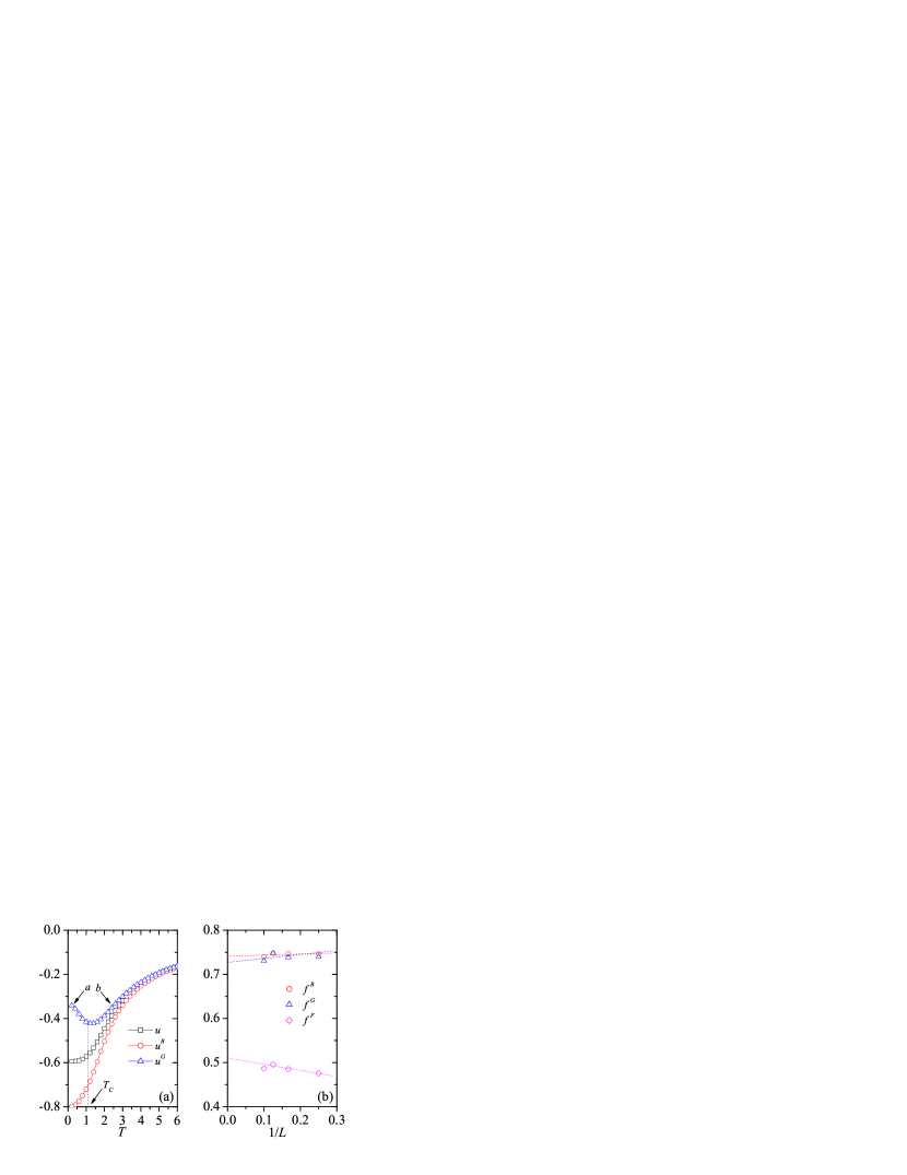
Figure 1: (Color online) (a) Average energies per bond $u$, $u^{B}$, and $u^{G}$, as function of $T$. Arrows indicate the critical temperature and two particular points on the $u^{G}$ curve, $a$ and $b$, located below and above $T_{c}$. (b) Average fractions of spins $f^{B}$, $f^{G}$, and $f^{F}$, as function of $1/L$.

Unlike bonds, separating the spins into groups may not be a trivial task. Typically two sets are chosen, the solidary spins which maintain their relative orientation in all configurations of the ground state and are connected by rigid bonds to each other, and the remaining ones that are called non-solidary spins. Although the backbone and the glass regions have roughly the same number of bonds, this separation produces two sets with very different fractions of spins: $77\%$ and $23\%$ of, respectively, solidary and non solidary spins. Such a rule was chosen because, a priori, the backbone was considered the most important structure in the system.

Here, assuming both the backbone and glass are of equal importance, we use these structures to separate the spins into two groups. We call $\Omega^{B}$ ($\Omega^{G}$) the set of spins connected to almost a rigid (flexible) bond, where the superscript $B$ ($G$) indicates that such region is dominated by the backbone (glass). Since some spins are connected to both rigid and flexible bonds these two sets intersect, $\Omega^{F}=\Omega^{B}\bigcap\Omega^{G}$, where now the superscript $F$ denotes the frontier between these structures.

In Fig. 1 (b) we can see the average fractions of spins that belong to the sets $\Omega^{B}$ ($f^{B}$), $\Omega^{G}$ ($f^{G}$), and $\Omega^{F}$ ($f^{F}$), as a function of $1/L$. A naive extrapolation to the thermodynamic limit indicates that these quantities tend approximately to $f^{B}\sim 0.74$, $f^{G}\sim 0.73$, and $f^{F}\sim 0.51$, which shows that the mean numbers of spins in the backbone and glass regions are very similar, and the frontier has half of the spins of the system, i. e., both structures interpenetrate each other sharing a region whose size is proportional to $N$.

III Critical behavior

After having separated the spins in different sets as described above, it is possible to analyze other observables within each of these regions. As usual, to study the critical behavior of the model we have calculated the Binder cumulant of the overlap order parameter and the correlation length (which also depends on the overlap between two replicas of the system, see below). The advantage of using these observables is that they allow one to determine the existence of a continuous phase transition regardless of the type of symmetry that is broken at the critical point. Nevertheless, we will only show results of the correlation length because, as is well known, unlike the Binder cumulant for small lattice sizes it allows one to determine the critical point with greater precision Katzgraber2006 .

The correlation length $\xi^{x}$ is defined as Palassini1999 (in cases where a given quantity is not calculated over the whole system, we use a superscript $x$ to indicate the region over which it is evaluated)

$$\xi^{x}=\frac{1}{2\sin(|\mathbf{k}_{\textrm{min}}|/2)}\Bigg{[}\frac{\chi^{x}(0)}{\chi^{x}(\mathbf{k}_{\textrm{min}})}-1\Bigg{]}^{1/2},$$ (2)

where $\mathbf{k}_{\textrm{min}}=(2\pi/L,0,0)$ is the smaller nonzero wave vector and $\chi^{x}(\mathbf{k})$ is the wave vector dependent spin-glass susceptibility,

$$\chi^{x}(\mathbf{k})=\frac{1}{N_{\Omega^{x}}}\sum_{i,j\in\Omega^{x}}[\langle q_{i}q_{j}\rangle_{T}]_{\textrm{av}}\ e^{\textrm{i}\mathbf{k}\cdot(\mathbf{r}_{i}-\mathbf{r}_{j})}.$$ (3)

Here, $q_{i}=\sigma_{i}^{\alpha}\sigma_{i}^{\beta}$ is the single spin overlap between two replicas of the system $\alpha$ and $\beta$, $N_{\Omega^{x}}$ is the number of spins of region $\Omega^{x}$, and $\mathbf{r}_{i}$ is the vector of the position of the $i$-th spin. $\langle\cdots\rangle_{T}$ and $[\cdots]_{\textrm{av}}$ represent, respectively, the thermal and disorder averages. The correlation length divided by $L$ is a dimensionless quantity which scales as Katzgraber2006

$$\frac{\xi^{x}}{L}=\tilde{S^{x}}[L^{1/\nu^{x}}(T-T_{c}^{x})/T_{c}^{x}],$$ (4)

where $\tilde{S^{x}}$ is a universal scaling function, $T_{c}^{x}$ is the critical temperature, and $\nu^{x}$ is a critical exponent nota1 . If the system experiences a phase transition, according to Eq. (4) the curves of $\xi^{x}/L$ for different lattice sizes should intersect at $T_{c}^{x}$.

Given the limitations under which we carry out this study, i. e., we only dispose of a limited number of samples of small sizes, it is not appropriate to analyze the critical behavior of the model by a standard scaling technique. In doing this, one obtains critical parameters (the critical temperature and critical exponents) whose values do not rival those already estimated previously using systems of much larger sizes Baity-Jesi2013 . Instead, we will focus on checking (trying to get good data collapses of the curves) whether the phase transitions observed under different conditions are compatible with the universality class of the 3D EA model. If, for a given case, it is not possible to do this well, then we will calculate a suitable set of critical parameters for that particular situation.

Figure 2(a) shows the correlation length calculated for the whole system, $\xi$, for different lattice sizes as indicated. The curves intersect at approximately the true critical temperature and, using precise values of $T_{c}=1.1019(29)$ and $\nu=2.562(42)$ taken from recent literature Baity-Jesi2013 , we obtain a good data collapse (see inset). This example shows that, despite the limitations of our calculations (performed for few samples of very small sizes), it is still possible to study the critical behavior of the model with a certain degree of accuracy.

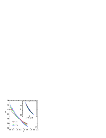
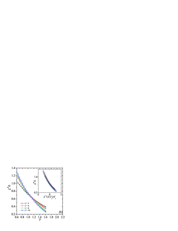
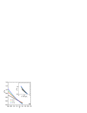
Figure 2: (Color online) Correlation length function divided by $L$ as function of $T$ for (a) the whole system, and for (b) the backbone and (c) glass regions. Insets show the corresponding data collapses performed according to Eq. (4) using the critical parameters $T_{c}=1.1019(29)$ and $\nu=2.562(42)$ Baity-Jesi2013 .

Now, we focus on the backbone and glass regions. Figure 2(b) shows that the curves of $\xi^{B}$ are very similar to those calculated for the whole system, and a good data collapse can be obtained using the same critical parameters as before (see inset). For the glass region, however, we do not obtain a result as robust as the previous one, see Fig. 2(c). Each pair of curves of $\xi^{G}$ calculated for two consecutive sizes intersect at a temperature slightly higher than $T_{c}$, and their crossing point slowly moves towards lower temperatures as the system size increases. The scaling plot shown in the inset, performed again using $T_{c}=1.1019(29)$ and $\nu=2.562(42)$, does not allow one to achieve a good data collapse. This suggests that the results obtained for the glass region are probably affected by very strong finite-size effects.

In order to determine with certainty the universality class of a phase transition, it is necessary to analyze the scaling of a second observable that depends on an independent critical exponent. Therefore, we calculate the spin-glass susceptibility, $\chi^{x}\equiv\chi^{x}[\mathbf{k}=(0,0,0)]$, for each of the regions considered as shown in Figs. 3(a), 3(b), and 3(c). Although for the whole system and the backbone we have obtained good data collapses of the correlation length using a conventional scaling Eq. (4), for the susceptibility we choose an extended scaling scheme Campbell2006

$$\chi^{x}=(LT)^{2-\eta^{x}}\tilde{C^{x}}[(LT)^{1/\nu^{x}}(1-(T_{c}^{x}/T^{x})^{2})],$$ (5)

which is more appropriate for dealing with samples of small sizes and, in addition to $\nu^{x}$, depends on the critical exponent $\eta^{x}$. Using the critical parameters of the 3D EA model, $T_{c}=1.1019(29)$, $\nu=2.562(42)$, and $\eta=-0.3900(36)$ Baity-Jesi2013 , we obtain excellent data collapses for all regions, and in particular for the glass one, see insets in Figs. 3(a), 3(b), and 3(c). Thus, we conclude that, despite what is observed in the Fig. 2(c), probably the critical behavior is the same in each of the regions in which we have divided the system.

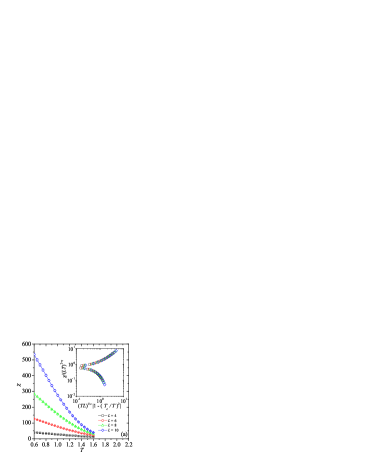
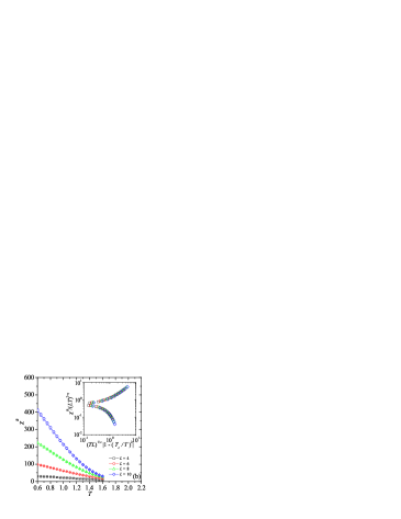
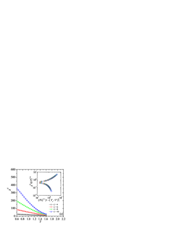
Figure 3: (Color online) Spin-glass susceptibility as function of $T$ for (a) the whole system, and for (b) the backbone and (c) glass regions. Insets show the corresponding data collapses (see text).

The previous results seem to suggest that the spatial heterogeneities we are considering are not closely related to the critical behavior of this system. This conclusion, however, is not entirely correct. As we shall see below, a selective bond dilution allows us to unveil surprising features of the backbone and glass regions, otherwise impossible to detect in a simulation that does not take into account such structures.

First, for comparison purposes, we calculate the correlation length and the spin-glass susceptibility for the 3D random bond-diluted EA spin-glass model, $\xi^{\ast}$ and $\chi^{\ast}$, Figs.  4(a) and 5(a), respectively. We use the same lattice sizes and number of samples as before, with $50\%$ of dilution. In Fig. 4(a) we can observe that the curves of $\xi^{\ast}/L$ cross at $T_{c}^{\ast}=0.75(1)$ and, using the critical exponents $\nu=2.562(42)$ and $\eta=-0.3900(36)$, good data collapses are obtained for this quantity (see inset) and for the spin-glass susceptibility, see inset in Fig. 5(a). This numerical experiment corroborates something that is well known, that a random bond dilution does not change the universality class of the 3D EA spin-glass model Hasenbusch2008 .

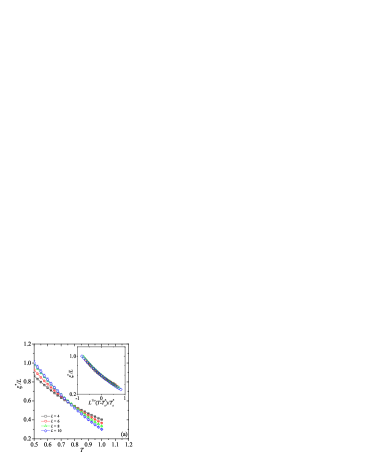
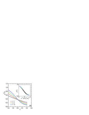
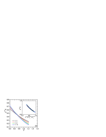
Figure 4: (Color online) Correlation length function divided by $L$ as function of $T$ for a random bond dilution (a) of $50\%$, and for a selective bond dilution of (b) the glass and (c) backbone regions. Insets show the corresponding data collapses (see text).

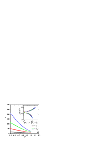
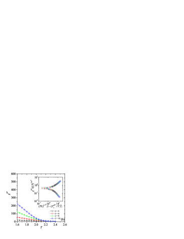
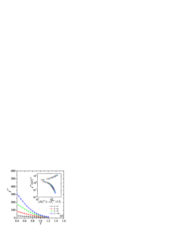
Figure 5: (Color online) Spin-glass susceptibility as function of $T$ for a random bond dilution (a) of $50\%$, and for a selective bond dilution of (b) the glass and (c) backbone regions. Insets show the corresponding data collapses (see text).

Surprisingly, a selective bond dilution is capable of inducing a change of universality. Figure 4(b) shows the correlation length curves calculated for the backbone region, $\xi^{B\ast}$, obtained after diluting the entire glass region. On one hand, we observe a cross at $T_{c}^{B\ast}=2.02(1)$, a critical temperature higher than that of the undiluted system. This is an expected result, since by removing the region with the greatest frustration of the system, the phase should be more stable in terms of energy and the critical temperature should rise. But, on the other hand, even more important is that when using the critical exponents of the 3D EA spin-glass model, we obtain very bad scaling plots that strongly suggesting that dilution produced a change in the universality class. Performing a careful statistical analysis of the data which is described in Appendix B, we calculate two new exponents for this particular case, $\nu^{B\ast}=0.81(1)$ and $\eta^{B\ast}=0.47(1)$. Using them, good data collapses are obtained for the correlation length [see inset in Fig. 4(b)] and for the corresponding spin-glass susceptibility, $\chi^{B\ast}$ [see inset in Fig. 5(b)]. Note that to calculate these values and their error bars we use a very limited number of small size samples available, so it is not easy to implement a method that allows taking into account systematic effects such as scale corrections. However, by using massive computational resources to improve data statistics and a standard procedure, it is possible that more precise critical exponents can be obtained that differ slightly from the values reported here.

In the opposite case, when we dilute the backbone but keep the glass region, we observe in Fig. 4(c) that the correlation length curves, $\xi^{G\ast}$, intersect at $T_{c}^{G\ast}=0.64(2)$. Unlike the previous case, this critical temperature is lower than $T_{c}$ since the most energetically stable region (backbone) has been removed. Using $\nu=2.562(42)$, the inset shows a much better data collapse than that obtained in the undiluted case [inset in Fig. 2(c)]. To confirm that this phase transition belongs to the universality class of the 3D EA spin-glass model, we make a scaling plot of the susceptibility, $\chi^{G\ast}$, using the exponent $\eta=-0.3900(36)$, which again leads to a very good data collapse, see inset in Fig. 5(c). In this way, it is justified that we have named this part of the system the glass region.

We emphasize the importance of these findings. We have been able to show that it is possible to change, or leave unaltered, the class of universality of the phase transition in the 3D EA spin-glass model by performing a selective bond dilution. This does not appear to be a spurious result since, as shown in Figs. 4 and 5, the data corresponding to these particular cases are not significantly influenced by finite-size effects. Furthermore, unlike what was done in the insets of these figures, as tested in Appendix C, if we try to collapse the curves for the backbone (glass) obtained after diluting the entire glass (backbone) region using the corresponding critical temperature, $T_{c}^{B\ast}$ ($T_{c}^{G\ast}$), but the set of exponents $\nu=2.562$ and $\eta=-0.39$ ($\nu^{B\ast}=0.81$ and $\eta^{B\ast}=0.47$), we obtain very bad scaling plots that reinforce the idea that the aforementioned change in the universality class is in fact real or at least very likely to be.

IV Ground-state energies

Finally, we observe that a selective bond dilution also affects other properties of the system, in particular its fundamental level. We calculate the probability distribution function, $P_{0}^{x}$, of ground-state energies per bond, $u_{0j}^{x}$, where as before the superscript $x$ indicates the region over which this energy is evaluated (unlike the previous cases, here we use the superscript $W$ to refer to the whole system) and the conditions under which the calculations are performed (the undiluted and diluted cases). Figure 6(a) presents the distributions that were obtained for samples of $L=10$, while the panel (b) shows the disorder average of each energy as function of $1/L$. Here, we can see important differences between the main regions of the system. In fact, a selective bond dilution of the glass region does not change the ground state of the backbone (the distributions of $u_{0j}^{B}$ and $u_{0j}^{B\ast}$ are equals), while in the opposite case an appreciable effect is observed: the probability distributions of $u_{0j}^{G}$ and $u_{0j}^{G\ast}$ are very different, and the latter overlaps appreciably with the corresponding one for the backbone. Therefore, a selective bond dilution can change the universality class of the phase transition of a given region leaving its ground state unchanged, and vice versa.

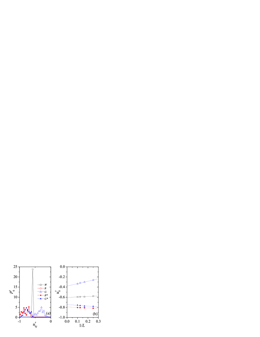
Figure 6: (Color online) Probability distribution functions of ground-state energies per bond for samples of $L=10$, and for the different regions as indicated. (b) Disorder average of these energies as function of $1/L$.

V Summary and conclusions

Summarizing, through an extensive analysis of the ground state of the 3D EA spin-glass model we have separated the system in two components, the backbone and the glass. We show that the phase transitions observed within each of these regions have the same class of universality than that has the whole system, i. e., in the first instance the spatial heterogeneities seem not to affect the critical behavior of the model. However, diluting the glass we observe that the ground state of the backbone remains unchanged but, more importantly, we detect that the universality class of the phase transition changes. In fact, we obtain two critical exponents, $\nu^{B\ast}=0.81(1)$ and $\eta^{B\ast}=0.47(1)$, that are very different from those of the 3D EA spin-glass model. In the opposite case, when the backbone is removed, we determine that the glass undergoes dramatic changes at its fundamental level, while the critical behavior remains the same as the undiluted system.

These results suggest that the critical behavior of the 3D EA spin-glass model originates from the interaction between two subsystems of very different nature, one of which dominates the other (the glass dominates over the backbone). Our analysis further reveals that there is no direct but subtle connection between the fundamental level of the model and this finite-temperature phenomenon: Selective dilution has an effect on the ground state that is opposite to the one it produces on the critical behavior. Further studies should be performed to clarify this issue.

Finally, it is important to mention that our results could be in conflict with the existence of chaos in temperature Fernandez2013 ; Katzgraber2007 . This phenomenon refers to the fragility of equilibrium configurations upon the slightest changes in temperature: It is to be expected that the overlap between two replicas of the system thermalized at two different but very closed temperatures tends to zero when the number of spins increases. In this context, our results showing, for small lattice sizes, that there is a connection between the fundamental level and the critical behavior (at finite temperature) of the 3D EA model, would not make sense at the thermodynamic limit. We note, however, that the backbone of a given sample is obtained from a very particular process: A bond is rigid (belong to the backbone) if it does not change its state, satisfied or frustrated, in all ground-state configurations. Therefore, this procedure allows one to determine a singular feature of the fundamental level that is not obtained from a standard equilibrium calculation, but arises from a comparison mechanism in which one or some particular configurations have the possibility of directly affecting its structure (in fact, if a bond changes its state in at least one configuration of the ground state, then said bond will be flexible). In addition, this information is used only for the purpose of separating each sample into two components. We then conjecture that our results may not be affected by the chaotic behavior of this spin-glass model Roma2013 . Nevertheless, further investigations similar to those carried out to study temperature chaos should be carried out to determine if this is the case.

Appendix A Monte Carlo simulations

Monte Carlo simulations are performed using a parallel tempering algorithm Geyer1991 ; Hukushima1996 . We use this technique to calculate both ground-state configurations Moreno2003 ; Roma2009 and average values of different observables at equilibrium, for $10^{4}$ samples for each size $L=4$ and $L=6$, $10^{3}$ for $L=8$, and $320$ for $L=10$.

This algorithm is implemented as follows. We simulate an ensemble of $M$ noninteracting replicas of a system of $N$ spins, each one associated to a different temperature in the interval $[T_{min},T_{max}]$ where, for simplicity, the difference between consecutive temperatures is chosen to be constant. A parallel tempering algorithm consists of two routines. One of them is a standard Monte Carlo procedure, i. e., an attempt to update a random selected spin of the ensemble (we randomly choose both a replica and a spin of this replica) with probability given by the Metropolis rule Metropolis . The second routine consists of an exchange of configurations between two replicas at consecutive temperatures which is attempted with the probability defined in Ref. Hukushima1996 . The unit time (or step) of a parallel tempering algorithm consists of $N\times M$ elementary steps of the standard Monte Carlo procedure, followed by a single trial of replica exchange.

For all cases, with the exception of the curves shown in Fig.1 (a), see below, the total simulation times (number of parallel tempering steps), $t$, required to equilibrate the system are chosen as $t=2\times 10^{5}$ for $L=4$, $t=4\times 10^{5}$ for $L=6$, $t=5\times 10^{5}$ for $L=8$, and $t=10^{6}$ for $L=10$. We also use between $M=17$ and $M=21$ replicas of the system in each case. To reach equilibrium under a given condition $x$ (the undiluted and diluted cases), as usual it is necessary to choose that the highest temperature is above the critical one, $T_{max}>T_{c}^{x}$. Once equilibrium is reached, the average values of different observables are calculated over a time interval of the same length $t$. In addition, equilibrium is tested by studying how the average values of all observables at all temperatures (but especially at $T_{min}$) change when $t$ is successively increased by factors of $2$, requiring that at least the last three results obtained coincide within the error bars.

In the particular case of Fig.1 (a), the curves are calculated only for $100$ samples of $L=10$ and $M=30$ replicas, which are simulated between $T_{max}=6.0$ and $T_{min}=0.2$. Because this last temperature is very low, to equilibrate we use $t=2\times 10^{6}$. We clarify that in this particular case the equilibrium was tested taking into account only the average energies per bond $u$, $u^{B}$, and $u^{G}$, and therefore other observables such as the corresponding correlation lengths might not have reached their equilibrium values for the lowest temperatures close to $T_{min}$. Nevertheless, note that the simulations corresponding to Figs. 2 to 5 were carried out independently and for temperature ranges different from those of Fig.1 (a).

In addition, it is necessary to find the backbone and glass regions of each realization of the quenched disorder. To determine which are the rigid and flexible bonds of a given sample, we use a very simple strategy Ramirez2004 ; Roma2010b :

1. A ground-state configuration $C$ is calculated and its energy $U_{0}$ is stored (to do this, we use a parallel tempering algorithm as explained in Ref. Roma2009 ).

2. Then, a bond $J_{ij}$ of the sample is chosen at random.

3. The system being in configuration $C$, one of the spins joined by the bond $J_{ij}$, i.e. either $\sigma_{i}$ or $\sigma_{j}$, is flipped. This flip changes the “condition” of the bond from satisfied to frustrated, or vice versa.

4. The orientations of the spins $i$ and $j$ are frozen and, for this “constrained” system, a new ground-state configuration $C^{\prime}$ of energy $U^{\prime}_{0}$ is calculated.

5. If $U^{\prime}_{0}>U_{0}$, it follows that $J_{ij}$ is a rigid bond (since we verify that there does not exist a ground-state configuration of energy $U_{0}$ in which this bond appears with its changed condition).

6. If $U^{\prime}=U$, then $J_{ij}$ is a flexible bond (we find a ground-state configuration of energy $U_{0}$ in which this bond appears with its changed condition; this configuration could have been found by exhaustively exploring the fundamental level of the unconstrained system).

7. The bond $J_{ij}$ is added to the list of “checked” bonds, and the restrictions over the spins $\sigma_{i}$ or $\sigma_{j}$ are lifted.

8. If there are still non-checked bonds, a new bond $J_{ij}$ is chosen among them and the process is repeated from step 3.

Ground-state configurations were calculated with the same parallel tempering algorithm as before, using the parameters given in Refs. Roma2009 ; Roma2010b . Note that in this case such a technique is not used to equilibrate the system but to quickly reach the fundamental level with a high probability.

Appendix B Statistical analysis of the data

After a selective bond dilution of the glass region, we observe that the backbone undergoes a phase transition that does not belong to the universality class of the 3D EA spin-glass model. To determine a suitable set of critical parameters $T_{c}^{B\ast}$, $\nu^{B\ast}$, and $\eta^{B\ast}$, we use a procedure similar to that reported in Refs. Katzgraber2006 ; Matoz2016 . First, we fit each curve of correlation length and susceptibility to a fifth-order polynomial. Working exclusively with these continuous functions, we calculate $T_{c}^{B\ast}$ and $\nu^{B\ast}$ looking for the values of these parameters that allow us to achieve the best data collapse of the correlation length using a conventional scaling, Eq. (4). In addition, to determine $\eta^{B\ast}$, we fix $T_{c}^{B\ast}$ and $\nu^{B\ast}$ to the values obtained previously and we follow a similar procedure for the spin-glass susceptibility, i. e., we look for the best data collapse of these curves but now using an extended scaling, Eq. (5). Finally, we calculate the error bars of these new critical parameters through a bootstrap method by generating $100$ random realizations with replacement as described in Ref. Katzgraber2006 .

Appendix C Exchanging the critical exponents

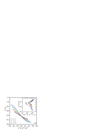
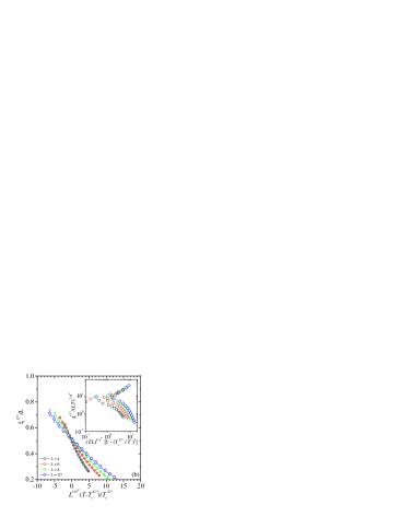
Figure 7: (Color online) Scaling plots of the correlation length curves (a) $\xi^{B\ast}$ and (b) $\xi^{G\ast}$ obtained using the corresponding critical temperatures, $T_{c}^{B\ast}=2.02$ and $T_{c}^{G\ast}=0.64$, and the exponents $\nu=2.562$ and $\nu^{B\ast}=0.81$, respectively. Insets show the scaling plots of the susceptibility curves (a) $\chi^{B\ast}$ and (b) $\chi^{G\ast}$, calculated with the previous sets of critical parameters, and using $\eta=-0.39$ and $\eta^{B\ast}=0.47$, respectively.

Figure 7(a) shows the scaling plot of the correlation length curves $\xi^{B\ast}$ obtained using the corresponding critical temperature, $T_{c}^{B\ast}=2.02$, and the exponent $\nu=2.562$. Clearly, we can observe the data is far from collapsing into a single universal curve. The same type of test is performed for the correlation length $\xi^{G\ast}$, in this case using $T_{c}^{G\ast}=0.64$ and $\nu^{B\ast}=0.81$. Again we obtain a very bad scaling plot, see Fig. 7(b). Similarly, the insets in these figures show the failed attempt to obtain good data collapses of susceptibility curves, using the exponent $\eta=-0.39$ for the backbone and $\eta^{B\ast}=0.47$ for the glass.

References

- (1) L. Berthier, G. Biroli, J.-P. Bouchaud, L. Cipelletti, and W. van Saarloos, Dynamical Heterogeneities in Glasses, Colloids, and Granular Media (Oxford Science Publishers, Oxford, 2011), Vol. 150.
- (2) W. K. Kegel and A. van Blaaderen, Science 287, 290 (2000).
- (3) E. R. Weeks, J. C. Crocker, A. C. Levitt, A. Schofield, and D. A. Weitz, Science 287, 627 (2000).
- (4) C. K. Mishra and R. Ganapathy, Phys. Rev. Lett. 114, 198302 (2015).
- (5) D. Heckendorf, K. J. Mutch, S. U. Egelhaaf, and M. Laurati, Phys. Rev. Lett. 119, 048003 (2017).
- (6) O. Dauchot, G. Marty, and G. Biroli, Phys. Rev. Lett. 95, 265701 (2005).
- (7) A. Ferguson and B. Chakraborty, Europhys. Lett. 78, 28003 (2007).
- (8) K. E. Avila, H. E. Castillo, A. Fiege, K. Vollmayr-Lee, and A. Zippelius, Phys. Rev. Lett. 113, 025701 (2014).
- (9) H. G. E. Hentschel, I. Procaccia, and S. Roy, Phys. Rev. E 100, 042902 (2019).
- (10) Y. Hiwatari and T. Muranaka, J. Non-Cryst. Solids 235–237, 19 (1998).
- (11) C. Bennemann, C. Donati, J. Caschnagel, and S. C. Glotzer, Nature (London) 399, 246 (1999).
- (12) L. Berthier, G. Biroli, J.-P. Bouchaud, L. Cipelletti, D. El Masri, D. L’Hôte, F. Ladieu, and M. Pierno, Science 310, 1797 (2005).
- (13) A. B. Kolton, D. R. Grempel, and D. Domínguez, Phys. Rev. B 71, 024206 (2005).
- (14) L. Wang, N. Xu, W. H. Wang, and P. Guan, Phys. Rev. Lett. 120, 125502 (2018).
- (15) T. Hoshino, S. Fujinami, T. Nakatani, and Y. Kohmura, Phys. Rev. Lett. 124, 118004 (2020).
- (16) K. Binder and A.P. Young, Rev. Mod. Phys. 58, 801 (1986).
- (17) K. H. Fischer and J. A. Hertz, Spin Glasses (Cambridge University Press, Cambridge, 1991).
- (18) S.F. Edwards and P.W. Anderson, J. Phys. F 5, 965 (1975).
- (19) F. Ricci-Tersenghi and R. Zecchina, Phys. Rev. E 62, R7567 (2000).
- (20) C. Chamon, M. P. Kennett, H. E. Castillo, and L. F. Cugliandolo, Phys. Rev. Lett. 89, 217201 (2002).
- (21) H. E. Castillo, C. Chamon, L. F. Cugliandolo, J. L. Iguain, and M. P. Kennett, Phys. Rev. B 68, 134442 (2003).
- (22) A. Montanari and F. Ricci-Tersenghi, Phys. Rev. Lett. 90, 017203 (2003).
- (23) F. Belletti, A. Cruz, L. A. Fernandez, A. Gordillo-Guerrero, M. Guidetti, A. Maiorano, F. Mantovani, E. Marinari, V. Martin-Mayor, J. Monforte, A. Muñoz Sudupe, D. Navarro, G. Parisi, S. Perez-Gaviro, J. J. Ruiz-Lorenzo, S. F. Schifano, D. Sciretti, A. Tarancon, R. Tripiccione, and D. Yllanes, J. of Stat. Phys. 135, 1121 (2009).
- (24) R. Alvarez Baños, A. Cruz, L. A. Fernandez, J. M. Gil-Narvion, A. Gordillo-Guerrero, M. Guidetti, A. Maiorano, F. Mantovani, E. Marinari, V. Martin-Mayor, J. Monforte-Garcia, A. Muñoz Sudupe, D. Navarro, G. Parisi, S. Perez-Gaviro, J. J. Ruiz-Lorenzo, S. F. Schifano, B. Seoane, A. Tarancon, R. Tripiccione, and D. Yllanes, Phys. Rev. Lett. 105, 177202 (2010).
- (25) L. A. Fernandez, V. Martin-Mayor, G. Parisi, and B. Seoane, Europhys. Lett. 103, 67003 (2013).
- (26) L. A. Fernandez, E. Marinari, V. Martin-Mayor, G. Parisi, and D. Yllanes, J. Stat. Mech.: Theo. Exp. 2016, 123301 (2016).
- (27) D. A. Mártin and J. L. Iguain, J. Stat. Mech.: Theo. Exp. 2017, 113302 (2017).
- (28) F. Romá, S. Bustingorry, and P. M. Gleiser, Phys. Rev. Lett. 96, 167205 (2006).
- (29) F. Romá, S. Bustingorry, P. M. Gleiser, and D. Domínguez, Phys. Rev. Lett. 98, 097203 (2007).
- (30) F. Romá, S. Bustingorry, and P. M. Gleiser, Eur. Phys. J. B 89, 259 (2016).
- (31) F. Barahona, R. Maynard, and R. Rammal, J. P. Uhry, J. Phys. A: Math. Gen. 15, 673 (1982).
- (32) F. Romá, S. Risau-Gusman, A. J. Ramirez-Pastor, F. Nieto, and E. E. Vogel, Phys. Rev. B 82, 214401 (2010).
- (33) F. Romá and S. Risau-Gusman, Phys. Rev. E 88, 042105 (2013).
- (34) R. Monasson, R. Zecchina, S. Kirkpatrick, B. Selman, and L. Troyansky, Nature (London) 400, 133 (1999).
- (35) S. Kirkpatrick, Phys. Rev. B 16,4630 (1977).
- (36) A. K. Hartmann, Phys. Rev. E 63, 016106 (2000).
- (37) C. Geyer, Computing Science and Statistics: Proceedings of the 23rd Symposium on the Interface (American Statistical Association, New York, 1991), p. 156.
- (38) K. Hukushima and K. Nemoto, J. Phys. Soc. Jpn. 65, 1604 (1996).
- (39) M. Baity-Jesi, R. A. Baños, A. Cruz, L. A. Fernandez, J. M. Gil-Narvion, A. Gordillo-Guerrero, D. Iñiguez, A. Maiorano, F. Mantovani, E. Marinari, V. Martin-Mayor, J. Monforte-Garcia, A. Muñoz Sudupe, D. Navarro, G. Parisi, S. Perez-Gaviro, M. Pivanti, F. Ricci-Tersenghi, J. J. Ruiz-Lorenzo, S. F. Schifano, B. Seoane, A. Tarancon, R. Tripiccione, and D. Yllanes, Phys. Rev. B 88, 224416 (2013).
- (40) H. G. Katzgraber, M. Körner, and A. P. Young, Phys. Rev. B 73, 224432 (2006).
- (41) M. Palassini and S. Caracciolo, Phys. Rev. Lett. 82, 5128 (1999).
- (42) Since when analyzing a certain region of the system the critical temperature and the critical exponents could change, to define them a superscript has been included. However, if any of these quantities has the same value as the corresponding critical parameter of the 3D EA model, then for simplicity the superscript is dropped.
- (43) I. A. Campbell, K. Hukushima, and H. Takayama, Phys. Rev. Lett. 97, 117202 (2006).
- (44) M. Hasenbusch, A. Pelissetto, and E. Vicari, Phys. Rev. B 78, 214205 (2008).
- (45) H. G. Katzgraber and F. Krza̧kała, Phys. Rev. Lett. 98, 017201 (2007).
- (46) J. L. Moreno, H. G. Katzgraber, and A. K. Hartmann, Int. J. Mod. Phys. C 14, 285 (2003).
- (47) F. Romá, S. Risau-Gusman, A. J. Ramirez-Pastor, F. Nieto, and E. E. Vogel, Physica A 388, 2821 (2009).
- (48) N. Metropolis, A. W. Rosenbluth, N. M. Rosenbluth, A. H. Teller, and E. Teller, J. Chem. Phys. 21, 1087 (1953).
- (49) A. J. Ramirez-Pastor, F. Romá, F. Nieto, and E. E. Vogel, Physica A 336, 454 (2004).
- (50) D. A. Matoz-Fernandez and F. Romá, Phys. Rev. B 94, 024201 (2016).