Generalized Lomb-Scargle analysis of $\rm{{}^{123}I}$ and $\rm{{}^{99m}Tc}$ decay rate measurements

Abstract

We apply the generalized Lomb-Scargle periodogram to the $\mathrm{{}^{123}I}$ and $\mathrm{{}^{99m}Tc}$ decay rate measurements based on data taken at the Bronson Methodist Hospital. The aim of this exercise was to carry out an independent search for sinusoidal modulation for these radionuclei (to complement the analysis in Borrello et al.) at frequencies for which other radionuclei have shown periodicities. We do not find such a modulation at any frequencies, including annual modulation or at frequencies associated with solar rotation. Our analysis codes and datasets have been made publicly available.

I Introduction

Over the past two decades, multiple groups (starting with Falkenberg Falkenberg (2001)), have argued for periodicities in the beta decay rates for various radioactive nuclei. Periodicities have been reported at 1 year (associated with the Earth-Sun distance) Jenkins et al. (2009); 28 days (associated with solar rotation) Sturrock et al. (2012, 2017), 29.5 days (associated with synodic lunar month) Parkhomov (2011), etc. Sturrock and Scargle (2001) have also found sinusoidal modulations in the solar neutrino data at the same frequencies. They have correlated these two sets of findings, and hence argued for the influence of solar rotation on the beta decay measurements. In addition to the above claims for a sinusoidal variation in the beta decay rates, correlations between beta decay rates and other transient astrophysical observations have also been found such as solar flares Jenkins and Fischbach (2009), and also the first binary neutron star merger seen in gravitational waves, GW170817 Fischbach et al. (2018). A review of some of these claims can be found in Jenkins et al. (2013); Sturrock et al. (2013, 2016, 2018).

However, other groups have failed to confirm these results, while analyzing the same data, or offered more prosaic explanations for the variability observed in the decay rate measurements. A review of some of the rejoinders and counter-rejoinders can be found in Jenkins et al. (2010); Sturrock et al. (2013, 2016, 2018); Kossert and Nähle (2015); Pommé et al. (2017, 2016, 2018); Pommé (2019); Pommé et al. (2018) and references therein. Other groups have also refuted the results related to an association between the beta decay rates and solar flares Bellotti et al. (2013); Angevaare et al. (2018). However, the jury is still out on some of these claims eg. the correlation between the decay rates of ³²Si and ³⁶Cl with GW170817 Fischbach et al. (2018), although no such correlations were seen in the decays of other nuclei, such as ⁴⁴Ti, ⁶⁰Co, and ¹³⁷Cs Breur et al. (2020). One impediment in reproducing some of these results, is that not all the beta-decay data and associated measurement errors have been made publicly available. To independently verify some of these claims, we have analyzed some of the beta-decay and solar neutrino data ourselves using robust statistical methods, for whatever data was accessible or made publicly available. Our analysis shows periodicities associated with solar rotation and annual modulation, although with a lower significance than claimed in some of the original works Desai and Liu (2016); Tejas and Desai (2018); Dhaygude and Desai (2020).

All the radioactive nuclei claimed to exhibit sinusoidal modulations are beta-decay emitters. Until recently, there was no study to check if any radionuclei which undergo isomeric transitions show variability, and only one study for nuclei undergoing electron capture O’Keefe et al. (2013). To rectify this, Borrello et al Borrello et al. (2018) (B18, hereafter) looked for periodicities in the decays of $\mathrm{{}^{123}I}$ (half-life of about 13 h) and $\mathrm{{}^{99m}Tc}$ (half-life of about 6 h). These radionuclides decay from electron capture and isomeric transition, respectively. Their decay chain is shown schematically in Fig. 1 and Fig. 2 of B18. These isotopes are widely used for clinical nuclear medicine purposes. Therefore, the widespread use of these isotopes in medical physics provides an another impetus to look for variability, since any deviation from a constant decay rate would also have implications for clinical studies. B18 applied the Lomb-Scargle periodogram to look for periodicities. From their analysis, no statistical significant peaks indicative of sinusoidal variations were found. They also did not find any correlation between their observed decay rates and solar activity as well as K-indices, which characterize the instability of Earth’s magnetic field.

In this work, we independently try to analyze the radioactive decay measurements in B18 (which were kindly provided to us by J. Borello) using the Generalized Lomb-Scargle periodogram Lomb (1976); Scargle (1982); Zechmeister and Kürster (2009) to look for any periodicities. Since the previous history of this field has shown that multiple groups analyzing the same data have reached drastically different conclusions Desai and Liu (2016); Tejas and Desai (2018); Dhaygude and Desai (2020), it behooves us to reanalyze this data and calculate significance of any possible periodicity using robust statistical techniques. We calculate the statistical significance of the most significant peak as well as other periods deemed interesting in literature, such as annual variation, solar rotation Sturrock et al. (2016, 2017), using multiple methods. For this analysis, we use the same methodology as in our previous work Dhaygude and Desai (2020).

The outline of this paper is as follows. We briefly recap some details of the Lomb-Scargle periodogram and different methods of calculating the false alarm probability in Sect. II. A brief summary of the results by B18 is discussed in Sect. III. Our own analysis is described in Sect. IV. We conclude in Sect. V.

II Generalized Lomb-Scargle Periodogram

The Lomb-Scargle (L-S) Lomb (1976); Scargle (1982); VanderPlas (2018); VanderPlas and Ivezić (2015); Ivezić et al. (2014) periodogram is a well-known technique to look for periodicities in unevenly sampled datasets. Its main goal is to determine the frequency ($f$) of a periodic signal in a time-series dataset $y(t)$ given by:

$$y(t)=a\cos(2\pi ft)+b\sin(2\pi ft).$$ (1)

The L-S periodogram calculates the power as a function of frequency, from which one can assess the statistical significance at a given frequency.

For this analysis, we use the generalized (or floating-mean) L-S periodogram Zechmeister and Kürster (2009); Bretthorst (2001). The main difference with respect to the ordinary L-S periodogram is that an arbitrary offset is added to the mean values. More details on the differences are elaborated in  VanderPlas (2018); VanderPlas and Ivezić (2015) and references therein. The generalized L-S periodogram has been shown to be more sensitive than the normal one, for detecting peaks, when the sampling of the data overestimates the mean VanderPlas (2018); Zechmeister and Kürster (2009); Vanderplas et al. (2012).

To evaluate the statistical significance of any peak in the L-S periodogram, we need to calculate its false alarm probability (FAP) or $p$-value. A large number of metrics have been developed to estimate the FAP of peaks in the L-S periodogram Scargle (1982); VanderPlas (2018); Pommé (2020); Pommé and De Hauwere (2020). We use most of these to calculate the FAP for our analysis. We now briefly describe enumerate these different techniques.

• Baluev

  This method uses extreme value statistics for stochastic process, to compute an upper-bound of the FAP for the alias-free case. The analytical expression for the FAP using this method can be found in  Baluev (2008); VanderPlas (2018).

• Bootstrap

  This method uses non-parametric bootstrap resampling VanderPlas (2018). It computes L-S periodograms on synthetic data for the same observation times. The bootstrap is the most robust estimate of the FAP, as it makes very few assumptions about the periodogram distribution, and the observed times also fully account for survey window effects VanderPlas (2018).

• Davies This method is similar to the Baluev method, but is not accurate at large false alarm probabilities, where it shows values greater than 1 Davies (2002).

• Naive

  This method is based on the ansatz that well-separated areas in the periodogram are independent. The total number of such independent frequencies depend on the sampling rate and total duration, and more details can be found in  VanderPlas (2018).

Once the FAP is known, based on any of the above methods, one can evaluate the $Z$-score or significance in terms of number of sigmas Cowan et al. (2011); Ganguly and Desai (2017), in case the FAP is very small. A rule of thumb for any peak to be interesting is that FAP is less than $0.05$. However for a peak to be statistically significant, its $Z-$score must be greater than 5$\sigma$.

III Recap of B18 and datasets used

Here, we briefly summarize the analysis in B18, wherein more details can be found. Their experiments were performed at the Bronson Methodist Hospital in Michigan. $\mathrm{{}^{123}I}$ (Iodine) was provided as sodium iodide crystals. The contamination from ¹²⁵I was deemed to be less than 12.4%. $\mathrm{{}^{99m}Tc}$ (Technetium) was supplied as sodium pertechnetate in aqueous solution with about 0.9% contamination from sodium chloride. More details about the apparatus and experimental procedure used for measuring the half-life can be found in B18. Half-life measurements were performed over a two-year period from May 2012 to June 2014. The mean time interval between $\mathrm{{}^{123}I}$ measurements was about 7 days 10 h, and the same for $\mathrm{{}^{99m}Tc}$ was 3 days 20 hr.

L-S analysis was then applied to the measured half-life data for both the radionuclides. A search for statistically significant peaks was done for both the nuclei upto 600 days. For $\mathrm{{}^{123}I}$ , the maximum significance occurs at a period of 23.5 days with $p$-value of 0.24. For $\mathrm{{}^{99m}Tc}$ , the maximum significance occurs at a period of 8.77 days with a $p$-value of 0.47. Therefore, no statistically significant peaks were seen. Then 95% c.l. upper limits were set on a periodic variation of one year. B18 then examined the outliers in the data for correlation with environmental factors, power supply voltage as well as for any outbursts in solar activity. No such correlations were seen. Therefore, B18 concludes that the $\mathrm{{}^{123}I}$ and $\mathrm{{}^{99m}Tc}$ data show no periodic variations, with limits on the amplitude of annual variation below 0.1% level.

IV Analysis and results

The $\mathrm{{}^{123}I}$ decay data comprise 101 measurements, of which one was discarded because of experimental disturbances. Similarly, the $\mathrm{{}^{99m}Tc}$ decay data comprise of 186 measurements, of which 11 were discarded because of an error in the sample preparation. Both these sets of decay measurements along with the associated errors were kindly made available to us by Dr. Borrello. The outliers were already removed from the dataset, so no additional pruning had to be done. These measurements are plotted in Fig. 1 and Fig. 2 for $\mathrm{{}^{99m}Tc}$ and $\mathrm{{}^{123}I}$ , respectively.

We now apply generalized L-S periodogram to this dataset. We used the L-S implementation in astropy Astropy Collaboration et al. (2018). For the frequency resolution and maximum frequency needed for the L-S analysis, we followed the recommendation in  VanderPlas (2018); viz. the size of each frequency bin is the reciprocal of five times the total duration of the dataset, and the maximum frequency is equal to five times the mean Nyquist equivalent frequency. Therefore, for $\mathrm{{}^{123}I}$ the frequency resolution is equal to 0.000269 day^-1 (0.098 year^-1) and maximum frequency equal to 0.337 day^-1 (123 year^-1). For $\mathrm{{}^{99m}Tc}$ , the corresponding numbers are 0.000268 day^-1 (0.098 year^-1) and 0.620 day^-1 (226.3 year^-1), respectively. However, since the astrophysically interesting frequencies are at 1/year and 8-14/year (associated with solar rotation) Sturrock et al. (2016, 2017), for brevity we only display the L-S periodogram upto a maximum range of 40/year. However, we also checked that there are no significant peaks at higher frequencies. We normalized the periodogram by the residuals of the data around the constant reference model. With this normalization, the L-S power varies between 0 and 1. This is similar to the normalization used in  Tejas and Desai (2018); Dhaygude and Desai (2020). On the other hand, B18 (also Desai and Liu (2016)) used the normalization proposed by Scargle Scargle (1982). The relation between these two normalizations is outlined in  Tejas and Desai (2018); VanderPlas (2018). The plots showing the L-S periodograms for $\mathrm{{}^{123}I}$ and $\mathrm{{}^{99m}Tc}$ can be found in Fig. 3 and Fig. 4, respectively. There are no huge peaks which stand out in these periodograms. Therefore, we find that our more sensitive method of looking for periodicities using the generalized L-S periodogram also does not reveal any significant peaks. However, we also quantify this by formally calculating the FAP using all the different methods outlined in Sect. II. The L-S powers, FAP (using all these methods) for the frequency with the maximum power, frequency associated with solar rotation, as well as that for annual modulation are shown in Table 1 and Table 2 for $\mathrm{{}^{99m}Tc}$ and $\mathrm{{}^{123}I}$ , respectively. For $\mathrm{{}^{99m}Tc}$ , the maximum power is seen at a period of about 11 days, with FAP (using bootstrap method) of about 0.9. For $\mathrm{{}^{123}I}$ , the maximum peak is seen at 23.39 days, with FAP (using the “Naive” method) of about 0.14. This corresponds to a $Z-$score of only 1.1$\sigma$, computed using the prescription in  Cowan et al. (2011); Ganguly and Desai (2017). As we can see, none of the FAPs are smaller than 0.05, and the FAP for frequencies associated with solar rotation as well as annual modulation are greater than 0.1.

Therefore, we concur with B18 that there are no periodicities in the nuclear decay rates for $\mathrm{{}^{123}I}$ and $\mathrm{{}^{99m}Tc}$ using the two year data accumulated at the Bronson Methodist hospital.

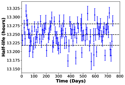
Figure 1: Half-life time-series (along with error bars) for $\mathrm{{}^{123}I}$ using the data from B18. The dashed horizontal lines indicate the $\pm 1\sigma$ range for the data.

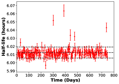
Figure 2: Half-life time-series for $\mathrm{{}^{99m}Tc}$ (along with error bars) using the data from B18. The dashed horizontal lines indicate the $\pm 1\sigma$ range for the data.

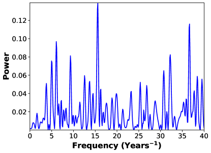
Figure 3: Generalized L-S periodogram for $\mathrm{{}^{123}I}$ shown upto frequency of 40/year. We also searched for statistically significant peaks at higher frequencies, upto 123/year, but did not find any.

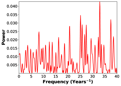
Figure 4: Generalized L-S periodogram for $\mathrm{{}^{123}I}$ shown upto frequency of 40/year. We also searched for statistically significant peaks at higher frequencies, upto 123/year, but did not find any.

Period (Days)	Frequency (year-1)	L-S Power	FAP : Baluev	FAP : Davies	FAP : Naive	FAP : Bootstrap
11.1	32.96	0.043	1.0	$>1.0$	0.99	0.920
354.8	1.03	0.00046	1.0	$>1.0$	1.0	1.0
44.6	8.18	0.025	1.0	$>1.0$	1.0	1.0

Table 1: $\mathrm{{}^{99m}Tc}$ L-S powers and FAP for our data using multiple methods: Baluev, Davies, Naive, and Bootstrap. We show the corresponding values of the period and frequency for the most significant peak (corresponding to the period of 11.07 days), followed by the period closest to the annual variation (365 days), as well as the period with maximum power in the solar rotation range (44.61 days). As we can see, all the FAPs are close to 1, and hence not significant.

Period (Days)	Frequency (year-1)	L-S Power	FAP : Baluev	FAP : Davies	FAP : Naive	FAP : Bootstrap
23.4	15.59	0.14	0.38	0.48	0.14	0.26
353.2	1.03	0.0056	1.0	$>1.0$	1.0	1.0
39.2	9.3	0.081	0.99	$>1.0$	0.98	0.998

Table 2: $\mathrm{{}^{123}I}$ L-S powers and FAP for our data using multiple methods: Baluev, Davies, Naive, and Bootstrap. Similar to Table 1, we find the corresponding values for the period and frequency of the most significant peak (corresponding to the period of 23.39 days), followed by the period closest to the annual variation (365 days), as well as the period with maximum power in the solar rotation range (39.24 days). As we can see, all the FAPs are $>$0.1, and are hence not significant. The peak with the maximum power (at 23.39 days) has the FAP of 0.14, corresponding to the $Z$-score of only 1.1$\sigma$.

V Conclusions

The aim of this work was to carry out an independent analysis of the $\mathrm{{}^{99m}Tc}$ and $\mathrm{{}^{123}I}$ nuclear decay rates, to look for statistically significant periodicities at frequencies, for which cyclic modulations have previously been found using other nuclei. The nuclear decay measurements were carried out in the Nuclear Medicine department at the Bronston Methodist Hospital in Michigan and are described in further detail in B18. $\mathrm{{}^{99m}Tc}$ and $\mathrm{{}^{123}I}$ decay by isomeric transitions and electron capture, respectively. Prior to this work, there were no searches for periodicities from nuclei with isomeric transitions, and only one search in case of electron capture.

For this purpose, we used the generalized or floating-mean L-S periodogram Zechmeister and Kürster (2009) (similar to our previous works Desai and Liu (2016); Tejas and Desai (2018); Dhaygude and Desai (2020)), as it is more sensitive than the ordinary L-S periodogram, which was used in B18. We searched for statistically significant peaks for both these nuclei upto five times the Nyquist frequency. This frequency range encompasses the band from 8 to 14 per year (which could contain signatures of influence from solar rotation) and also the annual modulation (in case of any influence due to the Earth-Sun distance).

The generalized L-S periodograms (upto a frequency range of 40/year) can be found in Fig. 3 and Fig. 4. The FAP for the highest peak, the frequency closest to one year, and also for the frequency with highest FAP between 8-14 per year can be found in Table 1 and Table 2. We do not find statistically significant peaks at any of these frequencies and the FAP for the peak with highest power is close to 1, indicating there is no periodicity at any frequency.

To promote transparency in data analysis, we have made our analysis codes and data available online, which can be found at https://github.com/Gautham-G/Lomb-Scargle-Analysis.