$f(R)$ Gravity Phase Space in the Presence of Thermal Effects

Abstract

In this paper, we shall consider $f(R)$ gravity and its cosmological implications, when an extra matter term generated by thermal effects is added by hand in the Lagrangian. We formulate the equations of motion of the theory as a dynamical system, that can be treated as an autonomous one only for specific solutions for the Hubble rate, which are of cosmological interest. Particularly, we focus our analysis on subspaces of the total phase space, corresponding to (quasi-)de Sitter accelerating expansion, matter-dominated and radiation-dominated solutions. In all the aforementioned cases, the dynamical system is an autonomous dynamical system. With regard to the thermal term effects, these are expected to significantly affect the evolution near a Big Rip singularity, and we also consider this case in terms of the corresponding dynamical system, in which case the system is non-autonomous, and we attempt to extract analytical and numerical solutions that can assess the specific cases. This course is taken twice: the first for the vacuum theory and the second when two perfect fluids (dust and radiation) are included as matter sources in the field equations. In both cases, we reach similar conclusions. The results of this theory do not differ significantly from the results of the pure $f(R)$ in the de Sitter and quasi-de Sitter phases, as the same fixed points are attained, so for sure the late-time era de Sitter is not affected. However, in the matter-dominated and radiation-dominated phases, the fixed points attained are affected by the presence of the thermal term, so surely the thermal effects would destroy the matter and radiation domination eras. However, with regard to the Big Rip case, several instabilities are found in the dynamical system, since the initial conditions dramatically affect the behavior of the dynamical system near the starting point of the $e$-foldings number evolution. Finally, we consider the effects of the thermal term on the late-time evolution of the Universe, by examining several statefinder quantities. Our findings indicate that these are reportable only under extreme fine tuning of the multiplicative coefficient of the thermal term.

I Introduction

Undoubtedly dark energy is one of the current mysteries in theoretical physics. The observation of the late-time acceleration driven by the mysterious dark energy in the late 90’s Riess:1998cb , still remains a firm proof that the Universe deviates in a major degree from the standard cosmological model described by general relativity. Modified gravity seems to harbor in a quite successful way the consistent description of the dark energy era reviews1 ; reviews2 ; reviews3 ; reviews4 ; reviews5 ; reviews6 and in some cases it is also possible to describe under the same theoretical framework the inflationary era and the dark energy era Odintsov:2020nwm ; Nojiri:2003ft . Nevertheless, until the generator of this dark energy fluid is found, current research also focuses on side effects related to the dark energy era. One first study in this respect, focused on the thermal effects caused in the Friedmann equation, of the form $\alpha H^{4}$ studied in Ref. Nojiri:2020sti . In this work we shall use the dynamical system approach Bahamonde:2017ize ; Oikonomou:2019muq ; Oikonomou:2019nmm ; Odintsov:2018uaw ; Odintsov:2018awm ; Boehmer:2014vea ; Bohmer:2010re ; Goheer:2007wu ; Leon:2014yua ; Guo:2013swa ; Leon:2010pu ; deSouza:2007zpn ; Giacomini:2017yuk ; Kofinas:2014aka ; Leon:2012mt ; Gonzalez:2006cj ; Alho:2016gzi ; Biswas:2015cva ; Muller:2014qja ; Mirza:2014nfa ; Rippl:1995bg ; Ivanov:2011vy ; Khurshudyan:2016qox ; Boko:2016mwr ; Odintsov:2017icc ; Granda:2017dlx ; Landim:2016gpz ; Landim:2015uda ; Landim:2016dxh ; Bari:2018edl ; Ganiou:2018dta ; Shah:2018qkh ; Oikonomou:2017ppp ; Odintsov:2017tbc ; Dutta:2017fjw ; Odintsov:2015wwp ; Kleidis:2018cdx ; Oikonomou:2019boy ; Chatzarakis:2019fbn . in order to reveal the effects of these thermal terms in subspaces of the total phase space of the cosmological system, with special cosmological interest. Our study will focus on $f(R)$ theories of gravity in vacuum or the presence of perfect matter fluids, and our aim is to reveal the structure of the phase space subspaces corresponding to (quasi) de Sitter, matter dominated or radiation dominated eras in the presence of an added by hand thermal term. We shall formulate the equations of motion of the theory as a dynamical system, that can be rendered as an autonomous dynamical system only for specific solutions for the Hubble rate, which are of cosmological interest. Specifically, we shall be interested in subspaces of the total phase space, corresponding to (quasi-)de Sitter accelerating expansion, matter-dominated and radiation-dominated solutions as we already mentioned, in which cases, the dynamical system can be rendered an autonomous dynamical system. With regard to the thermal term effects, these are expected to affect the evolution near a Big Rip singularity, and we also consider this case in terms of the corresponding dynamical system, in which case the system is non-autonomous, and we attempt to extract analytical and numerical solutions that can assess the specific cases. We perform all the aforementioned studies for both the vacuum theory and in the presence of perfect matter fluids (dust and radiation). In both cases, we reach similar conclusions. The results of this theory do not differ significantly from the results of the pure $f(R)$ in the de Sitter and quasi-de Sitter phases, as the same fixed points are attained. However, in the matter-dominated and radiation-dominated phases, the fixed points which we found are affected significantly by the presence of the thermal term, thus the matter and radiation domination eras are destroyed essentially by thermal effects. This clearly shows that these thermal terms should not be in the Lagrangian during these eras, as was expected. What we expected though is that the dynamical system would be strongly unstable for the Big Rip singularity, and our analysis exactly verified this result. Actually, in the Big Rip case, the dynamical system is strongly unstable, and the initial conditions seem to dramatically affect the behavior of the dynamical system near the starting point of the $e$-foldings number evolution. Finally, we consider the effects of the thermal term on the late-time evolution of the Universe (present time acceleration), by concretely examining several statefinder quantities, using a numerical approach. Our findings indicate that these are significant only under extreme fine tuning of the multiplicative coefficient $\alpha$ of the thermal term $\alpha H^{4}$. Thus with our results we verified that the thermal effects should only affect the cosmological evolution of $f(R)$ gravity near a Big Rip singularity and should not be present during the matter and radiation domination eras, since they would destroy all the desirable evolution properties during these deceleration eras. Also during the acceleration eras, materialized by (quasi) de Sitter fixed points, the thermal effects are insignificant, as the dynamical system study shows, or can affect the large redshift ($z\sim 6$) dark energy singularities, under extreme fine tuning, at least when viable models of $f(R)$ gravity are used.

The paper is organized as follows. In section II, we examine the case of the vacuum $f(R)$ gravity with an additional fluid term for the classical cosmological eras, whereas it can be modelled and analyzed as an autonomous dynamical system. The non-autonomous case is assessed in section III, where the finite-time singularities are considered. These two cases are considered again in the same manner in section IV where two perfect fluids are also included as matter sources in the field equations of the $f(R)$. In section V we study quantitatively the effects of the thermal terms on the late-time era by examining several late-time statefinder quantities. Finally, the conclusions follow at the end of the paper.

II The Case of the Vacuum $f(R)$ Autonomous System

It is known that near a Big Rip singularity, thermal effects may affect the cosmological evolution Nojiri:2020sti , since these might become significant due to the cosmological horizon “surrounding” the singularity. In this research line, we shall study in some detail the effects of the thermal terms on the dynamical system of $f(R)$ gravity. Let us commence our study by introducing the gravitational action and we shall consider the vacuum $f(R)$ gravity in the presence of thermal correction terms in the equation of motion, in which case the action is,

$$\centering S=\int{\mathrm{d^{4}x}\sqrt{-g}\left(\frac{f(R)}{2\kappa^{2}}+\mathcal{L}_{eff}\right)}\,,\@add@centering$$ (1)

where $g$ is the determinant of the metric tensor $g^{\mu\nu}$, $\kappa=\dfrac{1}{M_{P}}$ with $M_{P}$ being the reduced Planck mass, $f(R)$ is an arbitrary for the time being function of the Ricci scalar, which for a flat Friedmann-Robertson-Walker (FRW) background is given by the expression $R=6(2H^{2}+\dot{H})$ due to the flat cosmological background assumed. It is written as a function depending solely on Hubble’s parameter $H=\dfrac{\dot{a}}{a}$ where as usual $a(t)$ denotes the scale factor and the “dot” implies differentiation with respect to cosmic time $t$. Lastly $\mathcal{L}_{eff}$ is an additional term which quantifies the thermal effects on the late-time era. Its influence in the equations of motion will be shown explicitly in the equations of motion that now follow. In particular, by implementing the variation principle with respect to the metric tensor, one obtains the following equations of motion,

$$\centering 0=-\frac{f(R)}{2}+3(\dot{H}+H^{2})F(R)-18(4\dot{H}H^{2}+H\ddot{H})\frac{dF}{dR}+\alpha\kappa^{2}H^{4}\,,\@add@centering$$ (2)

where $F=\dfrac{\mathrm{d}f}{\mathrm{d}R}$. The extra term $\alpha\kappa^{2}H^{4}$ is produced by the effective fluid Lagrangian density $\mathcal{L}_{eff}$ that quantifies the thermal effects in Eq. (48) and its influence on the dynamics of the total cosmological fluid is the main subject of this paper. In order to form an appropriate dynamical system from the equations of motion, and study in detail the dynamics of the system, we introduce the following dimensionless dynamical variables,

$$\centering x_{1}\@add@centering =-\frac{\dot{F}}{HF} x_{2} =-\frac{f}{6FH^{2}} x_{3} =\frac{R}{6H^{2}} x_{4} =\frac{\alpha\kappa^{2}H^{2}}{3F}\,,$$ (3)

The first three variables are identical with the ones used in the case of vacuum $f(R)$ gravity Odintsov:2017tbc , hence the only new variable is the dynamical variable $x_{4}$. Genuinely speaking, it is introduced and chosen in this way on purpose, in order to rewrite Eq. (2) in terms of the dynamical variables elegantly as follows,

$$\centering x_{1}+x_{2}+x_{3}+x_{4}=1\,.\@add@centering$$ (4)

Let us now proceed with the construction of the dynamical system, which is non-linear in our case. In the following, we shall make use of the $e$-foldings number as a dynamical variable, instead of the cosmic time, in order to designate a new differential operator so as to replace the time derivatives. In principle, since $H=\dfrac{\mathrm{d}N}{\mathrm{dt}}$, the differential operator reads,

$$\centering\frac{\mathrm{d}}{\mathrm{dN}}=\frac{1}{H}\frac{\mathrm{d}}{\mathrm{dt}}\,,\@add@centering$$ (5)

In consequence, the non-linear dynamical system takes the following form,

$$\centering\frac{\mathrm{d}x_{1}}{\mathrm{dN}}=x_{1}(x_{1}+3-x_{3})+2(x_{3}-2)(1-2x_{4})\,,\@add@centering$$ (6)

$$\centering\frac{\mathrm{d}x_{2}}{\mathrm{dN}}=x_{2}(x_{1}-2x_{3}+4)-4(x_{3}-2)+m\,,\@add@centering$$ (7)

$$\centering\frac{\mathrm{d}x_{3}}{\mathrm{dN}}=-m-2(x_{3}-2)^{2}\,,\@add@centering$$ (8)

$$\centering\frac{\mathrm{d}x_{4}}{\mathrm{dN}}=x_{4}(x_{1}+2x_{3}-4)\,.\@add@centering$$ (9)

As expected, for $x_{4}\to 0$, one obtains the usual dynamical system for a pure $f(R)$ gravity in vacuum. In addition, we introduced a new parameter $m=-\dfrac{\ddot{H}}{H^{3}}$ which is of crucial importance in the following sections, as we now explain. Apparently, for a general solution for the Hubble rate $H(t)$, the parameter $m$ is time-dependent and hence, the dynamical system (6)-(9) is rendered non-autonomous. However, for several cosmological solutions of interest, the parameter $m$ takes constant values. Specifically, if the Hubble rate describes a quasi-de Sitter or a de Sitter evolution, or a matter or even a radiation dominated evolution, the parameter $m$ takes constant values. Specifically, these values will not be random but rather we shall showcase that three choices, namely $m=0$ and $m=-\dfrac{9}{2}$ and $m=-8$ result in decent descriptions of the inflationary era, the matter-dominated era and the radiation-dominated era respectively. These values are the same irrespective of the presence of the thermal effects generated terms. By assigning specific values on the parameter $m$ we actually investigate a subspace of the total phase space corresponding to the dynamical system. Practically, we do not fix the Hubble rate, but we rather investigate the behavior of the dynamical system for specific values of the parameter $m$, which in turn indeed correspond to several solutions of cosmological interest, thus we divide by hand the total phase space of the dynamical system, which by the way is impossible to study in a concrete way, to subspaces of cosmological interest. Our aim in this paper is to study what are the effects of the thermal terms $\sim H^{4}$, or equivalently of the variable $x_{4}$, on the dynamical system, focusing on the subspaces of the total phase space corresponding to the values of the parameter $m$ describing the quasi-de Sitter or de Sitter ($m=0$), the matter dominated era ($m=-\dfrac{9}{2}$) and the radiation dominated era ($m=-8$).

For a general constant value of the parameter $m$, there exist equilibria which are somewhat symmetric. In particular, the aforementioned fixed points are,

$$\phi_{*}^{1}=\left(\frac{1}{4}\left(-\sqrt{-2m}-2-\sqrt{4-2m+20\sqrt{-2m}}\right),\frac{1}{4}\left(3\sqrt{-2m}-2+\sqrt{4-2m+20\sqrt{-2m}}\right),2-\frac{\sqrt{-2m}}{4},0\right)$$ (10)

$$\phi_{*}^{2}=\left(\frac{1}{4}\left(-\sqrt{-2m}-2+\sqrt{4-2m+20\sqrt{-2m}}\right),\frac{1}{4}\left(3\sqrt{-2m}-2-\sqrt{4-2m+20\sqrt{-2m}}\right),2-\frac{\sqrt{-2m}}{4},0\right)$$

$$\phi_{*}^{3}=\left(\frac{1}{4}\left(\sqrt{-2m}-2-\sqrt{4-2m-20\sqrt{-2m}}\right),\frac{1}{4}\left(-3\sqrt{-2m}-2+\sqrt{4-2m-20\sqrt{-2m}}\right),2+\frac{\sqrt{-2m}}{4},0\right)$$

$$\phi_{*}^{4}=\left(\frac{1}{4}\left(\sqrt{-2m}-2+\sqrt{4-2m-20\sqrt{-2m}}\right),\frac{1}{4}\left(-3\sqrt{-2m}-2-\sqrt{4-2m-20\sqrt{-2m}}\right),2+\frac{\sqrt{-m}}{4},0\right)$$

$$\phi_{*}^{5}=\left(\sqrt{-2m},\frac{1}{4}\left(\sqrt{-2m}-4\right),2-\frac{\sqrt{-2m}}{4},-\frac{3}{2}\sqrt{\frac{-m}{2}}\right)$$

$$\phi_{*}^{6}=\left(-\sqrt{-2m},\dfrac{1}{2}\left(-4-\sqrt{-2m}\right),2+\frac{\sqrt{-2m}}{4},\frac{3}{2}\sqrt{\frac{-m}{2}}\right)\,.$$

It can easily be inferred that the third and sixth equilibrium points are the new ones derived from the inclusion of $\alpha H^{4}$ in Eq. (2), while the rest coincide with the equilibrium points of the pure vacuum $f(R)$ case Odintsov:2017tbc . Even though the points are the same, it is worth inspecting their stability once again, simply because the overall system has now been altered. In particular, the type of stability may not be changed but in order to ascertain this, we must inspect such a possibility. In the following, we shall examine the stability of each equilibrium point. Before doing so, we should note that all six equilibria fulfil the Friedmann constraint of Eq. (4), hence they are all viable cosmological solutions of the Friedmann equation.

In order to make a qualitative analysis, we shall make use of the Hartman-Grobman theorem, where basically the stability of a hyperbolic equilibrium point of a non-linear system is topologically equivalent to the stability of the linearized system in the neighborhood of the particular equilibrium point. Consequently, the (nonzero) eigenvalues of the Jacobian can account for the stability . From its definition, the Jacobian is given by the expression $J=\sum_{i,j}\frac{\partial f_{i}}{\partial x_{j}}$, where in the case at hand we have $f_{i}=\dfrac{\mathrm{d}x_{i}}{\mathrm{dN}}$. In particular, the Jacobian has the following form,

$$\centering J=\left(\begin{array}[]{cccc}2x^{*}_{1}-x^{*}_{3}+3&0&2(1-2x^{*}_{4})-x_{1}&-4(x^{*}_{3}-2)\\ x_{2}^{*}&x^{*}_{1}-2x^{*}_{3}+4&-4(x^{*}_{2}+2)&0\\ 0&0&-4(x^{*}_{3}-2)&0\\ x^{*}_{4}&0&2x^{*}_{4}&x^{*}_{1}+2x^{*}_{3}-4\\ \end{array}\right)\@add@centering$$ (11)

The Jacobian seems to be independent of the value of $m$, though it depends on the fixed points, and the fixed points can significantly be altered as $m$ changes. Hence, both the fixed points and the Jacobian change with respect to the free parameter $m$, indicating changes in the stability as well.

We are bound to omit $\phi_{*}^{3}$ and $\phi_{*}^{4}$, as they are complex for all $m\leq 0$, hence they have no physical interest as fixed points. Regarding the remaining four, we may reach the following conclusions:

Table 1: Equilibrium Points for the vacuum $f(R)$ autonomous system

Fixed Point	Eigenvalues	Characterization	Centre Manifolds
$\phi_{*}^{1}$	$\frac{1}{4}\left(-5\sqrt{-2m}-2-\sqrt{4-2m+20\sqrt{-2m}}\right)$, $\frac{1}{4}\left(3\sqrt{-2m}-2-\sqrt{4-2m+20\sqrt{-2m}}\right)$, $-\sqrt{1+5\sqrt{-2m}-\frac{m}{2}}$ and $2\sqrt{-2m}$	Saddle	For $m=0$ and $m=-8$
$\phi_{*}^{2}$	$\frac{1}{4}\left(-5\sqrt{-2m}-2+\sqrt{4-2m+20\sqrt{-2m}}\right)$, $\frac{1}{4}\left(3\sqrt{-2m}+\sqrt{-2m-2+20\sqrt{-2m}}\right)$, $\sqrt{1+5\sqrt{-2m}-\frac{m}{2}}$ and $2\sqrt{-2m}$	Saddle	For $m=0$
$\phi_{*}^{5}$	$\left(\right)$ $\frac{1}{4}\left(5\sqrt{-2m}+2-\sqrt{4-2m+20\sqrt{-2m}}\right)$, $\frac{1}{4}\left(5\sqrt{-2m}+2+\sqrt{-2m+2+20\sqrt{-2m}}\right)$, $2\sqrt{-2m}$ and $2\sqrt{-2m}$	Unstable Node	For $m=0$
$\phi_{*}^{6}$	$\frac{1}{4}\left(2-5\sqrt{-2m}-\sqrt{4-2m-20\sqrt{-2m}}\right)$, $\frac{1}{4}\left(-5\sqrt{-2m}+2+\sqrt{4-2m-20\sqrt{-2m}}\right)$, $-2\sqrt{-2m}$ and $-2\sqrt{-2m}$	Stable Node-Focus	For $m=0$

What we can see from Table 1 is that all equilibrium points yield at least one centre manifold, usually for $m=0$, which recall describes the quasi-de Sitter or de Sitter cosmological eras. Only in two cases does the centre manifold persist, in which cases a purely imaginary eigenvalue appears; it is easy to see, though, that this imaginary eigenvalue is not sufficient to alter the asymptotic stability of the particular fixed points, on the contrary it consolidates it. Furthermore, we observe that, in spite of bifurcations due to the constant values of the parameter $m$, the local stability of the equilibria is not affected. Consequently, different values of $m$ lead to a translocation of the equilibria in the phase space, but do not alter their stability. Finally, we see that $\phi_{*}^{6}$ is characterized by local asymptotic stability, hence it is expected to attract solutions and stand for a viable cosmological model. It is important to note that interestingly, this equilibrium $\phi_{*}^{6}$ is among the new ones, that have no counterpart in the pure vacuum $f(R)$ case.

Since one cannot draw any more conclusions from this general standpoint, we proceed by studying qualitatively and quantitatively (numerically) the subspaces of the phase space corresponding to the quasi-de Sitter or de Sitter ($m=0$), the matter dominated era ($m=-\dfrac{9}{2}$) and the radiation dominated era ($m=-8$) cases. Before that, however, it is worth mentioning that the system is partly integrable, noticing that Eq. (8) is independent of the other variables and integrable itself, as well as the fact that $x_{1}$ is bound to follow $x_{3}$ in specific cases.

II.1 The integrability of $x_{3}$

Eq. (8) is easily solved and the solution is,

$$x_{3}(N)=\frac{1}{2}\left(4-\sqrt{2m}\tan\left(\sqrt{2m}(N-N_{0})\right)\right)\,,$$ (12)

where $N_{0}$ stands for the initial $e$-foldings value (specifying the initial condition for $x_{3}$). Given specific values for $m$ and $N_{0}$, we see in Fig. (1) that $x_{3}$ always converges -within at most four $e$-foldings, to an equilibrium point given by,

$$x_{3}^{*}=2+\frac{\sqrt{-2m}}{2}\,.$$

The blue curves in Fig. (1) stand for $m=0$ (de Sitter expansion), the deep purple curves for $m=-\dfrac{9}{2}$ (matter-dominated cosmologies), the magenta curves for $m=-8$ (radiation-dominated cosmologies) and the red curves for $m=-9$ (stiff matter-dominated cosmologies), while solid, dashed and dotted curves depict increasing $N_{0}$; all cases exhibit the same behavior.

Figure 1: Analytic solutions of Eq. (8). Blue curves stand for $m=0$, purple curves for $m=-\dfrac{9}{2}$ and red ones for $m=-8$; the solid curves denote initial conditions for $N_{0}=0$, while dashing becomes thinner as $N_{0}>0$ grows.

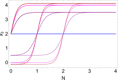
Interestingly, when $x_{3}=2$, which is true only in the (quasi) de Sitter expansion ($m=0$), the system of Eqs. (6), (7) and (9) is significantly simplified, becoming integrable as well. The solutions are,

$$x_{1}(N)=\dfrac{x_{1}(0)e^{N}}{1+x_{1}(0)\left(1-e^{N}\right)}\,,\;\;\;x_{2}(N)=\dfrac{x_{2}(0)}{1+x_{1}(0)\left(1-e^{N}\right)}\;\;\;\text{and}\;\;\;x_{4}(N)=\dfrac{x_{4}(0)}{1+x_{1}(0)\left(1-e^{N}\right)}\,,$$ (13)

where $x_{1}(0)$, $x_{2}(0)$ and $x_{4}(0)$ are arbitrarily chosen initial values; all solutions are naturally lead to the phase space points $x_{1}^{*}=-1$, $x_{2}^{*}=x_{4}^{*}=0$. The respective parametric solution is,

$$x_{2}=x_{2}(0)\left(1+x_{1}\right)\;\;\;\text{and}\;\;\;x_{4}=x_{4}(0)\left(1+x_{1}\right)\,,$$ (14)

that define integrals of motion in the hyperplane $x_{3}=2$ for $m=0$. An important comment here is that the phase space point $x_{1}^{*}=-1$, $x_{2}^{*}=x_{4}^{*}=0$ and $x_{3}=2$, was found to be a stable fixed point of the pure $f(R)$ gravity case Odintsov:2017tbc . In the next section we further highlight this important issue.

II.2 The case of de Sitter Expansion: $m=0$

Let us now proceed with the phase space behavior focusing on the subspace related to de Sitter or quasi-de Sitter solutions, which recall correspond to the specific value of $m$, that of $m=0$. From the realization that $x_{3}=2$ when $m=0$, we obtain that the deceleration parameter is exactly $q=-1$. Therefore, this choice is suitable for describing a de-Sitter (or quasi-de Sitter) expansion, that can describe both the inflationary and the late-time accelerating expansions. These two different eras can be described appropriately by choosing the final value of the $e$-foldings number to be large or small, describing the late or early time evolution of the Universe respectively. Also the initial value of the $e$-foldings number may play some role eventually, as we discuss in a later section, when the Big Rip singularity is considered.

For $m=0$, the equilibrium points extracted from Eq.(10) are,

$$\centering\phi_{*}^{1}=\@add@centering (-1,0,2,0) \phi_{*}^{2}= (0,-1,2,0)\,,$$ (15)

where for simplicity we neglected the rest, since they merely coincide with these two. The first yields the eigenvalues $\{-1,-1,0,-1\}$, where $\vec{v}_{1}=(1,0,0,0)$, $\vec{v}_{2}=(0,1,0,0)$ and $\vec{v}_{4}=(0,0,0,1)$ are tangent to the stable manifolds and a centre manifold appears to be tangent on $\vec{v}_{0}=(3,-4,1,0,0)$; seeing that the latter is removable from the system due to the $\vec{v}_{3}$ direction, we can characterize the equilibrium point as locally asymptotically stable. The second fixed point exhibits the eigenvalues $\{1,0,0,0\}$, where only $\vec{v}_{-1,1}=(-1,1,0,0)$ defines an unstable manifold, and with all the rest being tangent to centre manifolds, deeming the fixed point non-hyperbolic; as a result, we are unable to characterize these by using the Hartman-Grobman theorem.

Hence we easily come to the conclusion that when de Sitter or quasi-de Sitter solutions are considered, which correspond to the case $m=0$, the phase space substructure for the (quasi) de Sitter solutions is exactly the same as in the pure $f(R)$ vacuum case studied in Ref. Odintsov:2017tbc , where the term $\alpha H^{4}$ was absent. The solutions converge fast to the $x_{4}=0$ subspace, though numerical solutions seem to give an upper limit to this convergence, revealing the destabilizing role of the centre manifolds.

An interesting scenario occurs when the initial conditions are $x_{1},x_{2}>0$ and/or $x_{3}<2$, in which case the trajectory in the phase space for evolving $N$ is bound to diverge and tend to infinity. The initial conditions that respect these boundaries (hence for which $x_{1},x_{2}<0$ and $x_{3}>2$ - also $x_{4}>0$ so that we are consistent) converge rapidly to equilibrium $\phi_{*}^{1}$. The numerical solutions are depicted in Fig. 2, where the vector field corresponds to blue arrows, the numerical solutions as black curves and the equilibria are green dots. The first subplot depicts the $x_{1}-x_{2}$ slice of the phase space, the second subplot the $x_{1}-x_{3}$ slice, and finally the third the $x_{1}-x_{2}-x_{4}$ hyperplane for $x_{3}^{*}=2$.

Figure 2: The $x_{1}-x_{2}$, $x_{1}-x_{3}$ and $x_{1}-x_{2}-x_{4}$ subspaces of the phase space of the system of Eqs. (6-9) for $m=0$. Blue vectors stand for the vector field, black curves for the solutions, green dots for the equilibrium points and the red line for the heteroclinc orbit.

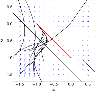
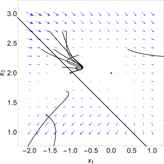
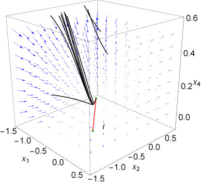
Another interesting situation occurs, by using the integrals defined by Eq. (14) and setting $x_{2}(0)=-1$ and $x_{4}(0)=0$, to match the unstable equilibrium point $\phi_{*}^{2}$. In this way, we obtain a heteroclinic trajectory towards the stable equilibrium point $\phi_{*}^{1}$, that functions as the unstable manifold of the former meets the stable manifold of the latter. This is marked with a straight red line in Fig. 2. This behavior is quite interesting since it shows that there is a trajectory in the (quasi) de Sitter subspace of the total phase space that actually connects the unstable fixed point $\phi_{*}^{2}$ with the stable fixed point $\phi_{*}^{1}$.

As we mentioned, only those trajectories whose initial values respect the rule $x_{1},x_{2}<0$ , $x_{3}>2$ and $x_{4}>0$ converge to the $\phi_{*}^{1}$, while all the other trajectories are led away by the instability of $\phi_{*}^{2}$. This is the outcome of the centre manifolds dominating the neighborhood of $\phi_{*}^{2}$. In fact, a higher-order approximation would deem it globally unstable.

These results conclude the examination of the (quasi) de Sitter solutions subspace of the total phase space. Our results indicate that the thermal terms do not affect significantly the de Sitter subspace of the total phase space, and thus, this means that no thermal effects can be considered of having a measurable effect on $f(R)$ gravity, even for late-time de Sitter solutions. To be honest, thermal effects would make their presence noticeable near a Big Rip singularity, not billion years before it. Thus our study verified our initial suspicion that such thermal effects do not affect the late-time era, at least when no Big Rip singularity is present. This is the phase space picture though, but a focused study on the late-time era observable quantities will show that for quite large values of $\alpha$ appearing in $\alpha\kappa^{2}H^{4}$, can actually alter the late-time behavior, even if this late-time era occurs quite far away from the Big Rip singularity, chronologically speaking.

Now in order to complete the phase space effects of the thermal terms, we shall analyze the subspaces of the total phase space corresponding to the matter and radiation dominated solutions. This is the subject of the following two subsections.

II.3 The case of Matter-Dominated Cosmologies: $m=-\dfrac{9}{2}$

The subspace of the total phase space corresponding to $m=-\dfrac{9}{2}$, describes the matter domination era, as we discussed earlier. In this section we shall investigate quantitatively the effects of the thermal term $\alpha\kappa^{2}H^{4}$ on the matter dominated solutions of the total phase space. In this case, the equilibrium points are,

$$\phi_{*}^{1}=\left(\frac{1}{4}\left(-5-\sqrt{73}\right),\frac{1}{4}\left(7+\sqrt{73}\right),\frac{1}{2},0\right)$$ (16)

$$\phi_{*}^{2}=\left(\frac{1}{4}\left(-5+\sqrt{73}\right),\frac{1}{4}\left(7-\sqrt{73}\right),\frac{1}{2},0\right)$$

$$\phi_{*}^{5}=\left(3,-\frac{1}{4},\frac{1}{2},-\frac{9}{4}\right)$$

$$\phi_{*}^{6}=\left(-3,-\frac{7}{4},\frac{7}{2},\frac{9}{4}\right)\,.$$

Here, two points are discarded, as they are complex and have no physical meaning and no other equivalence is observed. It is easily inferred that for $m=-\dfrac{9}{2}$, all fixed points are hyperbolic since the real part of the respective eigenvalues is nonzero.

More specifically, equilibria $\phi_{*}^{1}$ and $\phi^{*}_{2}$ yield the eigenvalues $\{-6.386,6,-4.272,-0.386001\}$ and $\{6,4.272,3.886,-2.114\}$ respectively, being both characterized as a saddles; interestingly, direction $\vec{v}_{2}=(0,-1,0,0)$ is always tangent to an unstable manifold. Equilibrium $\phi_{*}^{5}$ exhibits the eigenvalues $\{6.386,6,6,2.114\}$, all being positive, hence it is deemed an unstable node. Finally, equilibrium $\phi_{*}^{6}$ is found to be a stable node-focus, as its eigenvalues are $\{-6,-6,-3.25+1.71391i,-3.25-1.71391i\}$, two of them being real and negative also equal, hence a degeneracy is present, and the other two being complex with negative real part; solutions are expected to converge to the hyperplane parallel to $\vec{v}_{-1,2,4}=(-1.5095,0.3784,0,1)$ and then oscillate towards the fourth equilibrium point.

This behavior is clearly observed in Fig. 3, where again the vector field is denoted as blue arrows, the numerical solutions as black curves and the equilibria are green dots. In the second subplot, where an $x_{1}-x_{3}$ slice is shown, the solutions seem to converge simply on $x_{3}=3.5$ and then move towards the equilibrium, while in the first and third subplots, that depict the subspace orthogonal to $x_{3}$ direction, we clearly see the oscillating pattern; unfortunately, the convergence is too fast to see complete cyclical behavior.

Figure 3: The $x_{1}-x_{2}$, $x_{1}-x_{3}$ and $x_{1}-x_{2}-x_{4}$ subspaces of the phase space of the system of Eqs. (6-9) for $m=-\dfrac{9}{2}$. Blue vectors stand for the vector field, black curves for the solutions, green dots for the equilibrium points and the red line for the heteroclinc orbit.

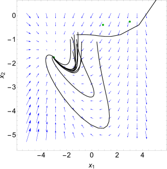
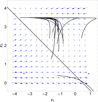
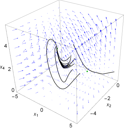
Interestingly, the equilibrium point attained is the only one with a viable (positive) nonzero value for $x_{4}$, while $\phi_{*}^{1}$ and $\phi_{*}^{2}$ that come along $x_{4}=0$, which describes the vacuum $f(R)$ theory. These are asymptotically unstable, repelling solutions to $x_{4}>0$. Consequently, the additional thermal term $\alpha\kappa^{2}H^{4}$ becomes important as we escape the inflationary era or the late-time accelerating expansion and we enter the more typical cases of matter dominated cosmologies. This result is quite intriguing since it shows that when a de Sitter era is followed by some matter dominated era, the thermal effects term may affect actually the dynamical evolution of the system, in the way we described in this subsection.

II.4 The case of Radiation-Dominated Cosmologies: $m=-8$

Now let us consider the effects of the thermal term $\alpha\kappa^{2}H^{4}$ on the phase space structure corresponding to radiation dominated solutions. The results for the radiation-dominated era are similar to those obtained for the matter-dominated solutions, as we now evince. Setting $m=-8$, a value which specifies the subspace of the total phase space corresponding to radiation dominated solutions, four equilibria are obtained,

$$\phi_{*}^{1}=\left(-4,5,0,0\right)$$ (17)

$$\phi_{*}^{2}=\left(1,0,0,0\right)$$

$$\phi_{*}^{5}=\left(4,0,0,-3\right)$$

$$\phi_{*}^{6}=\left(-4,-2,4,3\right)\,.$$

In the same manner, two points are discarded, as they are complex and have no physical meaning; all other fixed points are hyperbolic, as the real part of the respective eigenvalues is nonzero. As in the case of $m=-\dfrac{9}{2}$, the three first equilibria are asymptotically unstable, whereas $\phi_{*}^{6}$ is stable signifying a viable cosmological solution, which again comes with a positive value of $x_{4}$, hence it differs significantly from the vacuum $f(R)$ case. Specifically, the eigenvalues for $\phi_{*}^{1}$ and $\phi_{*}^{2}$ are $\{-8,8,-5,0\}$ and $\{8,5,5,-3\}$ respectively, deeming them saddles; again the $\vec{v}_{2}=(0,1,0,0)$ is tangent to an unstable manifold for the second, but a centre manifold exists for the first fixed point. The fixed point $\phi_{*}^{5}$ yields the eigenvalues $\{8,8,8,3\}$, so this fixed point is a degenerate unstable node. Finally, $\phi_{*}^{6}$ exhibits the eigenvalues $\{-8,-8,-4.5+1.93649i,-4.5-1.93649i\}$, hence it is a stable node-focus; the solutions are attracted by degenerate stable manifolds tangent to $\vec{v}_{-3,4}=(0,0,-4,3)$ and $\vec{v}_{2}=(0,1,0,0)$ to the hyperplane orthogonal to $\vec{v}_{-1,2,4}=(-1.5,0.5,0,1)$, where they oscillate towards the fixed point. In Fig. 4 we present the phase space behavior of several trajectories corresponding to radiation domination solutions.

Figure 4: The $x_{1}-x_{2}$, $x_{1}-x_{3}$ and $x_{1}-x_{2}-x_{4}$ subspaces of the phase space of the system of Eqs. (6-9) for $m=-8$. Blue vectors stand for the vector field, black curves for the solutions, green dots for the equilibrium points and the red line for the heteroclinic orbit.

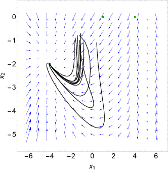
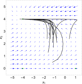
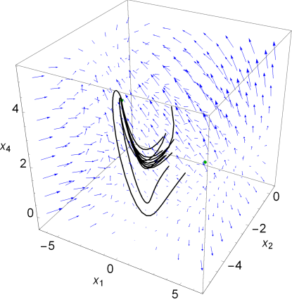
Our results indicate that the effects of the thermal terms on the matter and radiation dominated solutions of the total subspace, is significant, since the thermal term changes the phase space structure of vacuum $f(R)$ gravity. This is somewhat surprising to us, and also reportable result.

III The Case of the Vacuum $f(R)$ non-Autonomous System

The cases we examined so far where those that rendered the dynamical system of Eqs. (6)-(9) autonomous, those cases for which the Hubble rate had such a form as a function of time, that parameter $m$ takes constant values. However, this does not exhaust all interesting cases, especially the cases for which a finite-time singularity is approached at some time $t_{s}$. In this section we shall consider the Big Rip case, and we shall investigate the effects of the thermal term $\alpha H^{4}$ on the phase space of $f(R)$ gravity, as a Big Rip singularity is approached.

Following Ref. Nojiri:2005sx , we can assume that the Hubble rate is given as

$$H(t)\simeq H_{0}\left(t-t_{s}\right)^{-\beta}\,,$$ (18)

where $H_{0}$ some positive constant of dimension $sec^{\beta-1}$, and $\beta$ a free parameter that allows for the classification of the four types of singularities.

According to it, the Hubble rate reaches zero or infinity -depending on the values of $\beta$- whenever $t=t_{s}$; at this moment in time, some of the following singularities occur.

1. Type I Singularity (Big Rip), where $\beta>1$: In this case, the Universe expands so rapidly due to its growing content, that it is eventually “ripped apart”. All the scale factor, the total effective energy density and the total effective pressure of the Universe diverge strongly as $\beta\rightarrow\infty$, $\rho_{eff}\rightarrow\infty$ and $P_{eff}\rightarrow\infty$.

2. Type II Singularity (Sudden Death), where $-1<\beta<0$: In this case, the expansion of the Universe and the energy density of its content reach constant values, $\beta\rightarrow\beta_{s}$, $\rho_{eff}\rightarrow\rho_{s}$, however the total effective pressure approaches infinity, $P_{eff}\rightarrow\infty$.

3. Type III Singularity, where $0<\beta<1$: In this case, the Universe reaches a constant rate of expansion, but its actual or effective content continues to grow exponentially. Hence, while the scale factor reaches a constant value, $\beta\rightarrow\beta_{s}$, the total effective energy density and the total effective pressure blow up, $\rho_{eff}\rightarrow\infty$ and $P_{eff}\rightarrow\infty$.

4. Type IV Singularity, where $\beta<-1$: In this final case, the Universe and its content grow until a specific point, hence the scale factor, the total effective energy density and the total effective pressure simply reach constant values, $\beta\rightarrow\beta_{s}$, $\rho_{eff}\rightarrow\rho_{s}$ and $P_{eff}\rightarrow P_{s}$. However, the higher-than-second derivatives of the Hubble rate diverge. This is the only case of the finite-time singularities that a Universe may reach and smoothly pass through without being actually affected, or at least without being violently affected.

Rewriting the Hubble rate with respect to the $e$-foldings number, we have,

$$H(N)\simeq(1-\beta)\left(N-N_{c}\right)^{\frac{\beta}{\beta-1}}\,,$$ (19)

where $N_{c}$ is an integration constant, depending on the initial conditions. As a result, our parameter is no longer constant and depends on the $e$-foldings number, taking the form

$$m=-\dfrac{\beta(\beta+1)}{(\beta-1)^{2}\left(N_{c}-N\right)^{2}}\,.$$ (20)

Consequently, the system is no longer autonomous. Eqs. (6)-(9) now take the form,

$$\frac{\mathrm{d}x_{1}}{\mathrm{dN}} =x_{1}(x_{1}+3-x_{3})+2(x_{3}-2)(1-2x_{4})\,,$$ (21)

$$\frac{\mathrm{d}x_{2}}{\mathrm{dN}} =x_{2}(x_{1}-2x_{3}+4)-4(x_{3}-2)-\dfrac{\beta(\beta+1)}{(\beta-1)^{2}\left(N_{c}-N\right)^{2}}\,,$$

$$\frac{\mathrm{d}x_{3}}{\mathrm{dN}} =\dfrac{\beta(\beta+1)}{(\beta-1)^{2}\left(N_{c}-N\right)^{2}}-2(x_{3}-2)^{2}\;\;\;\text{and}$$

$$\frac{\mathrm{d}x_{4}}{\mathrm{dN}} =x_{4}(x_{1}+2x_{3}-4)\,.$$

This dynamical system cannot be analyzed qualitatively as we did so far, due to its “time-dependent” terms; it does not contain any fixed points or other invariant sets per se, but only as a special case, hence we may only proceed to either analytical or numerical solutions.

III.1 The “Big Rip” singularity

Depending on the nature of the finite-time singularity, we may simplify the parameter $m$. Concerning the Type I (Big Rip) singularity, we can utilize the approximation,

$$m\simeq-\dfrac{1}{\left(N_{c}-N\right)^{2}}\,.$$ (22)

In this case, $m$ approaches zero, as $N$ tends to infinity, which actually quantifies the effect of reaching the singularity. Simply stated, as $N\to\infty$, the Big Rip singularity is approached. The resulting dynamical system is identical to the one corresponding to the (quasi) de-Sitter study we performed in an earlier subsection. The value of $N_{c}$ itself plays an important role, as it defines the route by which the de Sitter phase will be reached, and thus whether it will be stable as we concluded above.

We can again see that Eq. (8) is analytically integrated, yielding in first order approximation close to $N_{c}$,

$$x_{3}(N)\simeq 2-\dfrac{1}{2(N-N_{c})}\,,$$ (23)

which approaches minus infinity as $N\rightarrow N_{c}$ and $2$ as $N\rightarrow\infty$. Utilizing this approximation of $x_{3}$ close to $N_{c}$, we can analytically integrate the complete system as

$$\begin{split}x_{1}(N)&=2+\dfrac{3e^{N_{c}}\left(2\sqrt{N_{c}}\mathcal{D}\left(\sqrt{N_{c}}\right)(2N_{c}(x_{1}(0)+1)-3)-2N_{c}(x_{1}(0)+1)-x_{1}(0)+2\right)}{\sqrt{-N_{c}}(2N_{c}(x_{1}(0)+1)-3)}\sqrt{N-N_{c}}+\\ &+12(N-N_{c})+\dfrac{15e^{N_{c}}\left(2\sqrt{N_{c}}\mathcal{D}\left(\sqrt{N_{c}}\right)(2N_{c}(x_{1}(0)+1)-3)-2N_{c}(x_{1}(0)+1)-x_{1}(0)+2\right)}{\sqrt{-N_{c}}(2N_{c}(x_{1}(0)+1)-3)}(N-N_{c})^{3/2}+\\ &+\left(40-\frac{6e^{2N_{c}}\left(-2\sqrt{N_{c}}\mathcal{D}\left(\sqrt{N_{c}}\right)(2N_{c}(x_{1}(0)+1)-3)+2N_{c}(x_{1}(0)+1)+x_{1}(0)-2\right)^{2}}{N_{c}(3-2N_{c}(x_{1}(0)+1))^{2}}\right)(N-N_{c})^{2}+\\ &+\dfrac{147e^{N_{c}}\left(2\sqrt{N_{c}}\mathcal{D}\left(\sqrt{N_{c}}\right)(2N_{c}(x_{1}(0)+1)-3)-2N_{c}(x_{1}(0)+1)-x_{1}(0)+2\right)}{2\sqrt{-N-c}(2N_{c}(x_{1}(0)+1)-3)}(N-N_{c})^{5/2}+\\ &+\mathcal{O}\left((N-N_{c})^{3}\right)\,,\end{split}$$ (24)

$$\begin{split}x_{2}(N)&=\dfrac{1}{2(N-N_{c})}-3+\dfrac{{3e^{N}_{c}}\left(\frac{2N_{c}(x_{1}(0)+1)+x_{1}(0)-2}{2N_{c}(x_{1}(0)+1)-3}-2\sqrt{N_{c}}\mathcal{D}\left(\sqrt{N_{c}}\right)\right)}{\sqrt{-N_{c}}}\sqrt{N-N_{c}}+\\ &+\dfrac{\left(6N_{c}\left(-8N_{c}^{2}(x_{1}(0)+1)+12N_{c}+x_{1}(0)+x_{2}(0)+1\right)+3\right)}{2N_{c}^{2}(2N_{c}(x_{1}(0)+1)-3)}(N-N_{c})-\\ &-\dfrac{15\left(e^{N_{c}}\left(2\sqrt{N_{c}}\mathcal{D}\left(\sqrt{N_{c}}\right)(2N_{c}(x_{1}(0)+1)-3)-2N_{c}(x_{1}(0)+1)-x_{1}(0)+2\right)\right)}{\sqrt{-N_{c}}(2N_{c}(x_{1}(0)+1)-3)}(N-N_{c})^{3/2}+\\ &+\mathcal{O}\left((N-N_{c})^{2}\right)\;\;\;\text{and}\end{split}$$ (25)

$$\begin{split}x_{3}(N)&=\dfrac{3N_{c}x_{4}(0)}{(N-N_{c})(2N_{c}(x_{1}(0)+1)-3)}+\dfrac{6N_{c}x_{4}(0)}{2N_{c}(x_{1}(0)+1)-3}-\\ &-\dfrac{6\left(e^{N_{c}}\sqrt{-N_{c}}x_{4}(0)\left(2\sqrt{N_{c}}\mathcal{D}\left(\sqrt{N_{c}}\right)(2N_{c}(x_{1}(0)+1)-3)-2N_{c}(x_{1}(0)+1)-x_{1}(0)+2\right)\right)}{(3-2N_{c}(x_{1}(0)+1))^{2}}\sqrt{N-N_{c}}+\\ &+\dfrac{24N_{c}x_{4}(0)}{2N_{c}(x_{1}(0)+1)-3}(N-N_{c})-\\ &-\dfrac{30\left(e^{N_{c}}\sqrt{-N_{c}}x_{4}(0)\left(2\sqrt{N_{c}}\mathcal{D}\left(\sqrt{N_{c}}\right)(2N_{c}(x_{1}(0)+1)-3)-2N_{c}(x_{1}(0)+1)-x_{1}(0)+2\right)\right)}{(3-2N_{c}(x_{1}(0)+1))^{2}}(N-N_{c})^{3/2}+\\ &+\mathcal{O}\left((N-N_{c})^{2}\right)\,,\end{split}$$ (26)

where $x_{1}(0)$, $x_{2}(0)$ and $x_{4}(0)$ are arbitrary initial conditions and $\mathcal{D}(z)=\left(e^{-z^{2}}\right)\int_{0}^{z}e^{y^{2}}\,dy$ is the Dawson integral function. As $x_{3}$ and $x_{4}$ approach $2$ and $0$ respectively, these solutions approach,

$$x_{1}(N)\simeq\dfrac{e^{N}x_{1}(0)}{x_{1}(0)\left(1-e^{N}\right)+1}\,,$$

$$x_{2}(N)\simeq\dfrac{e^{N_{c}}N_{c}x_{1}(0)(N_{c}-N)\left(\mathrm{Ei}(N-N_{c})-\mathrm{Ei}(-N_{c})\right)+\left(e^{N}-1\right)N_{c}x_{1}(0)+N_{c}x_{2}(0)(N_{c}-N)-N}{N_{c}(N-N_{c})\left(\left(e^{N}-1\right)x_{1}(0)-1\right)}\;\;\;\text{and}$$

$$x3(N)\simeq\dfrac{x_{4}(0)}{x_{1}(0)\left(1-e^{N}\right)+1}\,,$$

where $\mathrm{Ei}(z)=-\int_{-z}^{\infty}\dfrac{e^{-t}}{t}\,dt$ the exponential integral function.

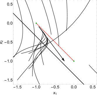
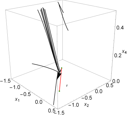
As we stated, for very large $N$, $m$ tends to zero, hence the de Sitter case should be reconstructed. However, this reconstruction depends highly on the value of $N_{c}$. For all physical values $N_{c}>0$, so the initial conditions of the system are set prior to $N_{c}$, the de Sitter case is not attained and the solutions diverge as $N\rightarrow N_{c}$; as we can see in Fig. 5, the solutions are originally attracted by the de Sitter stable fixed point, but then they are repelled, and the trajectories in the phase space are attracted by an unstable manifold.

This manifold can be located if we integrate analytically the system of Eqs. (6-8) for $x_{4}=0$ and $x_{3}=2-\dfrac{1}{(N-N_{c})^{2}}$ and assuming that $N\rightarrow N_{c}$; the manifold is indeed located as,

$$\bar{x}_{1}(N) =\dfrac{N_{c}+2(1-e^{N})}{N_{c}+2e^{N}(N-N_{c}-1)+2}\,,$$ (27)

$$\bar{x}_{2}(N) =\dfrac{5e^{N-N_{c}}(N-N_{c})(2-N_{c})\big{(}\mathrm{Ei}\left(N_{c}\right)-\mathrm{Ei}\left(N_{c}-N\right)\big{)}+5N_{c}-5N+1}{2e^{N}(2N_{c}-2N-2)-2N_{c}-4}+$$ (28)

$$+\dfrac{e^{N}\left(N^{2}(1-5N_{c})+10NN_{c}(N_{c}+1)+8N_{c}(N-N_{c})^{2}\ln\big{(}\frac{N_{c}-N}{N_{c}}\big{)}-N_{c}(N_{c}+2)(5N_{c}+1)\right)}{2N_{c}(N-N_{c})\left(2e^{N}(N-N_{c}-1)+N_{c}+2\right)}\;\;\;\text{and}$$ (29)

$$\bar{x}_{3}(N) =\frac{4NN_{c}-N-4N_{c}^{2}}{2N_{c}(N-N_{c})}\,.$$ (30)

Figure 5: The $x_{1}-x_{2}$, $x_{1}-x_{3}$ and $x_{1}-x_{2}-x_{4}$ subspaces of the phase space of the system of Eqs. (6-9) for $m=-\dfrac{1}{(N_{c}-N)^{2}}$ and $N_{c}>0$. Black curves for the solutions, green dots for the equilibrium points and the red line for the heteroclinc orbit.

IV Autonomous Dynamical System In the Presence of Perfect Fluids

In the previous section we studied the vacuum $f(R)$ gravity phase space subspaces corresponding to the (quasi) de Sitter, matter and radiation dominated eras, discussing mainly the case that these eras are generated by the vacuum $f(R)$ gravity. In this section we shall generalize the theoretical framework, by taking into account perfect fluids that can actually themselves can realize the matter and radiation domination eras. Thus the study and considerations of the previous sections are going to be generalized to include the presence of perfect fluids.

So in the presence of perfect matter fluids, the gravitational action reads,

$$\centering S=\int{d^{4}x\sqrt{-g}\left(\frac{f(R)}{2\kappa^{2}}+\mathcal{L}_{eff}+\mathcal{L}_{matter}\right)}\,,\@add@centering$$ (31)

where $\mathcal{L}_{matter}$ is the Lagrangian corresponding to perfect matter fluids. The inclusion of matter in the gravitational action results in the emergence of the energy densities of the perfect fluids in the equations of motion, with the Friedmann equation becoming,

$$\centering 0=-\frac{f(R)}{2}+3F(\dot{H}+H^{2})-18(4H^{2}\dot{H}+H\ddot{H})\frac{dF}{dR}+\alpha\kappa^{2}H^{2}+\kappa^{2}\rho_{matter}\,,\@add@centering$$ (32)

where $\rho_{matter}=\rho_{m}+\rho_{r}$ is the energy density for both non relativistic (dust) and relativistic (radiation) matter respectively. Regarding the dynamical system corresponding to the total cosmological system, in addition to the variables introduced in Eq. (3), the following two variables must be added,

$$\centering x_{5}\@add@centering =\frac{\kappa^{2}\rho_{r}}{3FH^{2}} x_{6} =\frac{\kappa^{2}\rho_{m}}{3FH^{2}}\,,$$ (33)

so by taking these two into account, the Friedmann constraint that must be satisfied by all the trajectories in the phase space, becomes,

$$\centering x_{1}+x_{2}+x_{3}+x_{4}+x_{5}+x_{6}=1\,.\@add@centering$$ (34)

Thus, the new dynamical system corresponding to the cosmological system at hand is now written as,

$$\centering\frac{dx_{1}}{dN}=x_{1}(x_{1}+3-x_{3})+2(x_{3}-2)(1-2x_{4})+4x_{5}+3x_{6}\,,\@add@centering$$ (35)

$$\centering\frac{dx_{2}}{dN}=x_{2}(x_{1}-2x_{3}+4)-4(x_{3}-2)+m\,,\@add@centering$$ (36)

$$\centering\frac{dx_{3}}{dN}=-m-2(x_{3}-2)^{2}\,,\@add@centering$$ (37)

$$\centering\frac{dx_{4}}{dN}=x_{4}(x_{1}+2x_{3}-4)\,,\@add@centering$$ (38)

$$\centering\frac{dx_{5}}{dN}=x_{5}(x_{1}-2x_{3})\,,\@add@centering$$ (39)

$$\centering\frac{dx_{6}}{dN}=x_{6}(x_{1}-2x_{3}+1)\,.\@add@centering$$ (40)

As mentioned previously, the system is autonomous only if $m$ is specified accordingly. As in the previous section, we shall choose the values $m=0$ for the (quasi) de Sitter expansion, $m=-\dfrac{9}{2}$ for the matter-dominated era, and $m=-8$ for the radiation-dominated era. In the case at hand, the radiation and matter domination eras can be realized by the corresponding perfect fluids, and not necessarily from the $f(R)$ gravity.

The equilibrium points of the dynamical system are now increased to ten, and these are,

$$\phi_{*}^{1}=\left(3-\sqrt{-2m},\dfrac{1}{3}\left(-m-2\sqrt{-2m}\right),2-\frac{\sqrt{-2m}}{2},0,0,\dfrac{1}{6}\left(2m-24+13\sqrt{-2m}\right)\right)$$ (41)

$$\phi_{*}^{2}=\left(4-\sqrt{-2m},-\dfrac{m+2\sqrt{-2m}}{4},2-\frac{\sqrt{-2m}}{2},0,\dfrac{1}{4}\left(m-20+8\sqrt{-2m}\right),0\right)$$

$$\phi_{*}^{3}=\left(3+\sqrt{-2m},\dfrac{1}{3}\left(m-2\sqrt{-2m}\right),2+\frac{\sqrt{-2m}}{2},0,0,\dfrac{1}{6}\left(2m-24-13\sqrt{-2m}\right)\right)$$

$$\phi_{*}^{4}=\left(4+\sqrt{-2m},-\dfrac{m-2\sqrt{-2m}}{4},2+\frac{\sqrt{-2m}}{2},0,\dfrac{1}{4}\left(m-20-8\sqrt{-2m}\right),0\right)$$

$$\phi_{*}^{5}=\left(\frac{1}{4}\left(-2-\sqrt{-2m}-\sqrt{4-2m+20\sqrt{-2m}}\right),\frac{1}{4}\left(-2+3\sqrt{-2m}+\sqrt{4-2m+20\sqrt{-2m}}\right),2-\frac{\sqrt{-2m}}{2},0,0,0\right)$$

$$\phi_{*}^{6}=\left(\frac{1}{4}\left(-2-\sqrt{-2m}+\sqrt{4-2m+20\sqrt{-2m}}\right),\frac{1}{4}\left(-2+3\sqrt{-2m}-\sqrt{4-2m+20\sqrt{-2m}}\right),2-\frac{\sqrt{-2m}}{2},0,0,0\right)$$

$$\phi_{*}^{7}=\left(\frac{1}{4}\left(-2+\sqrt{-2m}-\sqrt{4-2m+20\sqrt{-2m}}\right),\frac{1}{4}\left(-2-3\sqrt{-2m}+\sqrt{4-2m+20\sqrt{-2m}}\right),2+\frac{\sqrt{-2m}}{2},0,0,0\right)$$

$$\phi_{*}^{8}=\left(\frac{1}{4}\left(-2+\sqrt{-2m}+\sqrt{4-2m+20\sqrt{-2m}}\right),\frac{1}{4}\left(-2-3\sqrt{-2m}-\sqrt{4-2m+20\sqrt{-2m}}\right),2+\frac{\sqrt{-2m}}{2},0,0,0\right)$$

$$\phi_{*}^{9}=\left(\sqrt{-2m},\frac{1}{4}\left(-4+\sqrt{-2m}\right),2-\frac{\sqrt{-2m}}{2},-\frac{3\sqrt{-2m}}{4},0,0\right)$$

$$\phi_{*}^{10}=\left(-\sqrt{-2m},-\dfrac{1}{4}\left(4+\sqrt{-2m}\right),2+\dfrac{\sqrt{-2m}}{2},\dfrac{3\sqrt{-2m}}{4},0,0\right)\,.$$

In the presence of the matter fields, four extra fixed points emerge for general values of $m$, however -as was the case with the vacuum $f(R)$ model- many points may coincide while other may be discarded as being intrinsically unrealistic. In fact, at least two of them -namely $\phi_{*}^{7}$ and $\phi_{*}^{8}$- will indeed be discarded since these are complex. All the remaining eight are viable, as they fulfill the Friedmann constraint of Eq. (34).

The Jacobian for the dynamical system of Eqs. (35)-(39) reads,

$$\centering J=\left(\begin{array}[]{cccccc}2x_{1}^{*}-x_{3}^{*}+3&0&2(1-2x_{4}^{*})-x_{1}^{*}&-4(x_{3}^{*}-2)&4&3\\ x_{2}^{*}&x_{1}^{*}-2x_{3}^{*}+4&-2x_{2}^{*}-4&0&0&0\\ 0&0&-4(x_{3}^{*}-2)&0&0&0\\ x_{4}^{*}&0&2x_{4}^{*}&x_{1}^{*}+2x_{3}^{*}-4&0&0\\ x_{5}^{*}&0&-2x_{5}^{*}&0&x_{1}^{*}-2x_{3}^{*}&0\\ x_{6}^{*}&0&-2x_{6}^{*}&0&0&x_{1}^{*}-2x_{3}^{*}+1\\ \end{array}\right)\,,\@add@centering$$ (42)

again seeming independent of $m$, however the dependence of the fixed points on the parameter $m$ brings up the indirect dependence of the Jacobian as well, thus the position and the stability properties of the equilibria alter upon changes of the free parameter $m$. Dealing with the general case of linearizing around all ten fixed points (for $m\leq 0$) is complicated, yet the results are presented in table 2 -again, we have omitted two points that are complex, hence of no physical meaning. We observe that only one of the equilibria is asymptotically stable for all values of $m$, hence we naturally expect the solutions to be drawn to it. Not surprisingly, it is a reflection of the equilibrium for the vacuum case, where $x_{4}$ takes a nonzero value, while $x_{5}$ and $x_{6}$ are zero, hence the energy densities of dust and radiation are bound to decrease.

Table 2: Equilibrium Points for the $f(R)$-perfect fluids autonomous system

Fixed Point	Eigenvalues	Characterization	Centre Manifolds
Fixed Point	Eigenvalues	Characterization	Centre Manifolds
$\phi_{*}^{1}$	$3$ , $-1,\dfrac{1}{4}\left(14-3\sqrt{-2m}-\sqrt{4-2m+20\sqrt{-2m}}\right)$ , $\dfrac{1}{4}\left(14-3\sqrt{-2m}+\sqrt{4-2m+20\sqrt{-2m}}\right)$ , $3-2\sqrt{-2m}$ and $2\sqrt{-2m}$	Saddle	For $m=0$ and $m=-\dfrac{9}{8}$ and $m=-\dfrac{5}{2}$.
$\phi_{*}^{2}$	$4$ , $1$ , $\dfrac{1}{4}\left(18-3\sqrt{-2m}-\sqrt{4-2m+20\sqrt{-2m}}\right)$ , $\dfrac{1}{4}\left(18-3\sqrt{-2m}+\sqrt{4-2m+20\sqrt{-2m}}\right)$ , $4-2\sqrt{-2m}$ and $2\sqrt{2}\sqrt{-m}$	Saddle	For $m=0$, $m=-2$ and $m=-4.80816$.
$\phi_{*}^{3}$	$3$ , $-1$ , $3+2\sqrt{-2m}$ , $\dfrac{1}{4}\left(14+3\sqrt{-2m}-\sqrt{-2m-20\sqrt{-2m}+4}\right)$ , $\dfrac{1}{4}\left(14+3\sqrt{-2m}+\sqrt{4-2m-20\sqrt{-2m}}\right)$ and $-2\sqrt{-2m}$	Generalized Saddle	For all $m=0$.
$\phi_{*}^{4}$	$4$ , $1$ , $4+2\sqrt{-2m}$ , $\dfrac{1}{4}\left(18+3\sqrt{-2m}-\sqrt{4-2m-20\sqrt{-2m}}\right)$ , $\dfrac{1}{4}\left(18+3\sqrt{-2m}+\sqrt{4-2m-20\sqrt{-2m}}\right)$ and $-2\sqrt{-2m}$	Generalized Saddle	For all $m=0$.
$\phi_{*}^{5}$	$\dfrac{1}{4}\left(-2-5\sqrt{-2m}-\sqrt{4-2m+20\sqrt{-2m}}\right)$ , $\dfrac{1}{4}\left(-18+3\sqrt{-2m}-\sqrt{4-2m+20\sqrt{-2m}}\right)$ , $\dfrac{1}{4}\left(-14+3\sqrt{-2m}-\sqrt{4-2m+20\sqrt{-2m}}\right)$ , $\dfrac{1}{4}\left(-2+3\sqrt{-2m}-\sqrt{4-2m+20\sqrt{-2m}}\right)$ , $-\sqrt{1+5\sqrt{-2m}-\dfrac{m}{2}}$ and $2\sqrt{-2m}$	Saddle	For $m=0$ and $m=-8$.
$\phi_{*}^{6}$	$\dfrac{1}{4}\left(-2-5\sqrt{-2m}+\sqrt{4-2m+20\sqrt{-2m}}\right)$ , $\dfrac{1}{4}\left(-18+3\sqrt{-2m}+\sqrt{4-2m+20\sqrt{-2m}}\right)$ , $\dfrac{1}{4}\left(-14+3\sqrt{-2m}+\sqrt{4-2m+20\sqrt{-2m}}\right)$ , $\dfrac{1}{4}\left(-2+3\sqrt{-2m}+\sqrt{4-2m+20\sqrt{-2m}}\right)$ , $\sqrt{1+5\sqrt{-2m}-\frac{m}{2}}$ and $2\sqrt{-2m}$	Saddle	For $m=0$, $m=-2$ and $m=-4.80816$.
$\phi_{*}^{9}$	$-4+2\sqrt{-2m}$ , $-3+2\sqrt{-2m}$ , $2\sqrt{-2m}$ , $s_{1}$ , $s_{2}$ and $s_{3}$*	Saddle turning to Unstable Node	For $m=0$, $m=-\dfrac{9}{8}$ and $m=-2$.
$\phi_{*}^{10}$	$-4-2\sqrt{-2m}$ , $-3-2\sqrt{-2m}$ , $-2\sqrt{-2m}$ , $\tilde{s}_{1}$ , $\tilde{s}_{2}$ and $\tilde{s}_{3}$**	Stable Node-Focus	For $m=0$, $m=-6.52827$.
* Roots of polynomial $s^{3}+\left(-18\sqrt{-2m}-4\right)s^{2}+\left(32\sqrt{-2m}-208m\right)s+384m\sqrt{-2m}$.
** Roots of polynomial $\tilde{s}^{3}+\left(18\sqrt{-2m}-4\right)\tilde{s}^{2}+\left(-32\sqrt{-2m}-208m\right)\tilde{s}-384m\sqrt{-2m}$.

What we should notice, before moving towards the specific cosmological eras, specified by the values of $m$, is that whatever said for Eq. (8) holds for Eq. (37), as they are identical; these equations are decoupled from the system and integrated analytically producing the solutions noted in Fig. 1. This is particularly important for this case, as it may also decouple Eqs. (39) and (40). As the rates of change of $x_{5}$ and $x_{6}$ dependent only on $x_{1}$ and $x_{3}$, they will converge or diverge depending on whether the expression $x_{1}-2x_{3}+1$ is smaller than $-1$. Given that $x_{3}$ converges rapidly at $2+\dfrac{\sqrt{-2m}}{2}$ if $x_{3}>2-\dfrac{\sqrt{-2m}}{2}$, then we easily see that $x_{1}$ is also bounded by,

$$x_{1}<2+\sqrt{-2m}\,.$$

Interestingly, the value $x_{1}$ takes at the stable fixed point $\phi_{*}^{10}$ is $-2\left(2+\sqrt{-2m}\right)$, which is below that bound.

Ensuring that our initial conditions respect $x_{1}<2+\sqrt{-2m}$, $x_{3}>2-\dfrac{\sqrt{-2m}}{2}$ and $x_{4}$, $x_{5}$, $x_{6}\geq 0$, as well as the Friedmann constraint, we ensure that $\phi_{*}^{10}$ is reached normally. We clearly see from that how the centre and unstable manifolds divide the phase space -yet again- and force specific initial conditions in order for a viable solution to exist.

IV.1 The case of de Sitter Expansion: $m=0$

Now let us study the subspace of the total phase space of the cosmological system that corresponds to (quasi) de Sitter solutions, so for $m=0$. In this case, the fixed points of the dynamical system are,

$$\centering\phi_{*}^{1}\@add@centering (3,0,2,0,0,-4) \phi_{*}^{2} (4,0,2,0,-5,0) \phi_{*}^{5} (-1,0,2,0,0,0) \phi_{*}^{6}(0,-1,2,0,0,0)\,.$$ (43)

As it was mentioned earlier, the total number of equilibrium points is decreased and essentially there exist only four, out of total eight, and the rest are identical to these. Concerning the eigenvalues of Eq. (42) for each of these points, we can mention the following: Equilibrium $\phi_{*}^{1}$ yields $\{4,3,3,3,-1,0\}$, being a saddle with $\vec{v}_{-1,6}=(-3,0,0,0,0,4)$, $\vec{v}_{2}=(0,1,0,0,0,0)$ and $\vec{v}_{4}=(0,0,0,1,0,0)$ being tangent to the degenerate unstable manifolds, $\vec{v}_{1,-5,6}=(1,0,0,0,-5,4)$ to the stable manifold, and $\vec{v}_{0}=(-6,-4,-3,0,0,13)$ to a centre manifold. Equilibrium $\phi_{*}^{2}$ is characterized as a degenerate unstable node, with its eigenvalues being $\{5,4,4,4,1,0\}$ and $\vec{v}_{0}=(3,-4,1,0,0,0)$ being tangent to its only centre manifold. Equilibrium $\phi_{*}^{5}$ is a degenerate stable node, as the eigenvalues of Eq. (42) for it are $\{-5,-4,-1,-1,-1,0\}$, with $\vec{v}_{1}=(1,0,0,0,0,0)$, $\vec{v}_{2}=(0,1,0,0,0,0)$ and $\vec{v}_{4}=(0,0,0,1,0,0)$ denoting the degenerate stable manifolds and $\vec{v}_{0}=(-6,-4,-3,0,0,13)$ the corresponding centre manifold. Finally, $\phi_{*}^{6}$ is a saddle dominated by centre manifolds, since the eigenvalues are $\{-4,-3,1,0,0,0\}$. Notably, three centre manifolds appear tangent to directions $\vec{v}_{-1,-3}=(-2,0,-1,0,0,0)$, $\vec{v}_{2}=(0,1,0,0,0,0)$ and $\vec{v}_{4}=(0,0,0,1,0,0)$.

Consequently, the solutions are expected to converge to $\phi_{*}^{5}$ as long as the discussed bounds are considered. As in the previous case, we can see that $x_{3}=2$ even for very small values of the dynamical evolving variable $N$. In this case, the system of Eqs. (35), (36), (38) (39) and (40) is simplified and can be integrated, yielding,

$$x_{1}(N)= \dfrac{x_{1}(0)e^{N}}{1+x_{1}(0)\left(1-e^{N}\right)}\,,\;\;\;x_{2}(N)=\dfrac{x_{2}(0)}{1+x_{1}(0)\left(1-e^{N}\right)}\,,\;\;\;x_{4}(N)=\dfrac{x_{4}(0)}{1+x_{1}(0)\left(1-e^{N}\right)}\,,$$ (44)

$$x_{5}(N)=\dfrac{x_{5}(0)e^{-4N}}{1+x_{1}(0)\left(1-e^{N}\right)}\;\;\;\text{and}\;\;\;x_{6}(N)=\dfrac{x_{6}(0)e^{-3N}}{1+x_{1}(0)\left(1-e^{N}\right)}\,,$$

where $x_{1}(0)$, $x_{2}(0)$, $x_{4}(0)$ $x_{5}(0)$ and $x_{6}(0)$ are the initial values. All solutions are naturally led to the fixed point. On the $x_{1}-x_{2}-x_{4}$ hyperplane, the parametric solution of Eqs. (14) is valid, defining the respective stable manifold -as in the vacuum case. The overall behavior can easily be seen in Fig. 2, where the solutions do indeed follow this pattern, attracted and led to equilibrium point $\phi_{5}^{*}$. Obviously, any solutions whose initial conditions do not respect the afore-mentioned limitations are repelled away, as in the vacuum case.

IV.2 The case of Matter-Dominated Cosmologies: $m=-\frac{9}{2}$

Setting $m=-\dfrac{9}{2}$, we transcend to the matter-dominated era, where all eight equilibria appear, which are,

$$\phi_{*}^{1}=\left(0,-\frac{1}{2},\frac{1}{2},0,0,1\right)$$ (45)

$$\phi_{*}^{2}=\left(1,-\frac{3}{8},\frac{1}{2},0,-\frac{1}{8},0\right)$$

$$\phi_{*}^{3}=\left(6,\frac{7}{2},\frac{7}{2},0,0,-12\right)$$

$$\phi_{*}^{4}=\left(7,\frac{21}{8},\frac{7}{2},0,-\frac{97}{8},0\right)$$

$$\phi_{*}^{5}=\left(\frac{1}{4}\left(5-\sqrt{73}\right),\frac{1}{4}\left(7+\sqrt{73}\right),\frac{1}{2},0,0,0\right)$$

$$\phi_{*}^{6}=\left(\frac{1}{4}\left(-5+\sqrt{73}\right),\frac{1}{4}\left(7-\sqrt{73}\right),\frac{1}{2},0,0,0\right)$$

$$\phi_{*}^{7}=\left(3,-\frac{1}{4},\frac{1}{2},-\frac{9}{4},0,0\right)$$

$$\phi_{*}^{8}=\left(-3,-\frac{7}{4},\frac{7}{2},\frac{9}{4},0,0\right)\,,$$

Concerning their stability, we can draw the following conclusions from the linearization of the system in the neighborhood of each. The fixed points $\phi_{*}^{1}$ and $\phi_{*}^{2}$ exhibit eigenvalues $\{6,3.386,3,-3,-1,-0.886001\}$ and $\{6,4.386,4,-2,1,0.113999\}$, hence they are typical saddles, whereas for $\phi_{*}^{3}$ and $\phi_{*}^{4}$ we obtain eigenvalues $\{9,-6,5.75+1.71391i,5.75-1.71391i,3,-1\}$ and $\{10,6.75+1.71391i,6.75-1.71391i,-6,4,1\}$ respectively, so these are characterized as generalized saddles. The linearizations around $\phi_{*}^{5}$ result to the eigenvalues $\{-6.386,6,-4.386,-4.272,-3.386,-0.386001\}$, while for $\phi_{*}^{6}$ we have $\{6,4.272,3.886,-2.114,0.886001,-0.113999\}$, thus they are both saddles. Finally, the Jacobian in the neighborhood of the equilibrium point $\phi_{*}^{7}$ yields eigenvalues $\{6.386,6,6,3,2.114,2\}$, making it an unstable node, whereas in the neighborhood of equilibrium $\phi_{*}^{8}$ we get, $\{-10,-9,-6,-6,-3.25+1.71391i,-3.25-1.71391i\}$, making $\phi_{*}^{8}$ a stable node-focus. Both possess a degeneracy over the $\vec{v}_{2}=(0,1,0,0,0,0)$ direction.

As in the vacuum case, the solutions whose initial values follow the restrictions are attracted to the plane defined orthogonally to $\vec{v}_{-1,2,4}=(-1.44444,0.444444,0,1,0,0)$ and there they oscillate towards the stable fixed point. The oscillations depend of the real and the imaginary part of the sixth and fifth eigenvalue of $\phi_{*}^{8}$. Subsequently, the cyclical behavior is very small in comparison to the attraction. Thus the $x_{1}-x_{2}-x_{4}$ slice of the phase space of the system is identical to that of the previous system, as it is shown in Fig. 3.

The nonzero value of $x_{4}$ is preserved at this fixed point, regardless of the perfect fluids present, whose cosmological parameters are drawn to zero, usually within a few $e$-foldings -as the numerical solutions show. As a result, it is the thermal term $\sim\alpha H^{4}$ that characterized the respective viable cosmological solutions, rather than the matter fields themselves. However, the values of $x_{1}$ and $x_{2}$ differ significantly from the corresponding viable solutions in the vacuum case, indicating the role the matter fields play in the functional form of the $f(R)$ gravity actually.

IV.3 The case of Radiation-Dominated Cosmologies: $m=-8$

In much the same manner, when we set $m=-8$ that corresponds to the radiation-dominated era, we have the following eight equilibrium points,

$$\phi_{*}^{1}=\left(-1,0,0,0,0,2\right)$$ (46)

$$\phi_{*}^{2}=\left(0,0,0,0,1,0\right)$$

$$\phi_{*}^{3}=\left(7,\dfrac{16}{3},4,0,0,-\dfrac{46}{3}\right)$$

$$\phi_{*}^{4}=\left(8,4,4,0,-15,0\right)$$

$$\phi_{*}^{5}=\left(-4,5,0,0,0,0\right)$$

$$\phi_{*}^{6}=\left(1,0,0,0,0,0\right)$$

$$\phi_{*}^{7}=\left(4,0,0,-3,0,0\right)$$

$$\phi_{*}^{8}=\left(-4,-2,4,3,0,0\right)\,,$$

Given the Jacobian of Eq. (42) for each of them, we can demonstrate their stability characterization. The fixed points $\phi_{*}^{1}$ and $\phi_{2}^{*}$ are saddles, as the respective eigenvalues are $\{8,-5,3,3,-2,-1\}$ and $\{8,4,4,-4,1,-1\}$. It is noteworthy that direction $\vec{v}_{2}=(0,1,0,0,0,0)$ denotes a degenerate unstable manifold for both the fixed points. The fixed points $\phi_{3}^{*}$ and $\phi_{*}^{4}$ are characterized as generalized saddles, since they exhibit eigenvalues $\{11,-8,6.5+1.93649i,6.5-1.93649i,3,-1\}$ and $\{12,-8,7.5+1.93649i,7.5-1.93649i,4,1\}$ respectively, while $\phi_{*}^{6}$ is also a typical saddle with eigenvalues $\{8,5,5,-3,2,1\}$ with a degeneracy over $\vec{v}_{1}=(1,0,0,0,0,0)$ and $\vec{v}_{2}=(0,1,0,0,0,0)$ directions. The fixed point $\phi_{*}^{5}$ is yet another saddle, which however possesses a centre manifold, as its eigenvalues are $\{-8,8,-5,-4,-3,0\}$. The centre manifold is tangent to $\vec{v}_{2}=(0,1,0,0,0,0)$. Equilibrium $\phi_{*}^{7}$ is characterized by eigenvalues $\{8,8,8,5,4,3\}$ and hence it is thus a degenerate unstable node. Finally, equilibrium $\phi_{*}^{8}$ is a stable node-focus, as the linearized system around it yields $\{-12,-11,-8,-8,-4.5+1.93649i,-4.5-1.93649i\}$. Interestingly, directions $\vec{v}_{-3,4}=(0,0,-4,3,0,0)$ and $\vec{v}_{2}=(0,1,0,0,0,0)$ are tangent to degenerate unstable manifolds, due to the equality of the respective eigenvalues.

Thus in general, the numerical behavior of the trajectories in the case at hand, are similar to those depicted in Fig. 4.

IV.4 Non-autonomous Dynamical System in the Presence of Perfect Fluids

Finally, it is worth extending the Big Rip discussion of a previous section, in the case that perfect matter fluids are present, in which case the dynamical system becomes,

$$\frac{\mathrm{d}x_{1}}{\mathrm{dN}} =x_{1}(x_{1}+3-x_{3})+2(x_{3}-2)(1-2x_{4})+4x_{5}+3x_{6}\,,$$ (47)

$$\frac{\mathrm{d}x_{2}}{\mathrm{dN}} =x_{2}(x_{1}-2x_{3}+4)-4(x_{3}-2)-\dfrac{\beta(\beta+1)}{(\beta-1)^{2}\left(N_{c}-N\right)^{2}}\,,$$

$$\frac{\mathrm{d}x_{3}}{\mathrm{dN}} =\dfrac{\beta(\beta+1)}{(\beta-1)^{2}\left(N_{c}-N\right)^{2}}-2(x_{3}-2)^{2}\,,$$

$$\frac{\mathrm{d}x_{4}}{\mathrm{dN}} =x_{4}(x_{1}+2x_{3}-4)\,,$$

$$\frac{dx_{5}}{dN} =x_{5}(x_{1}-2x_{3})\;\;\;\text{and}$$

$$\frac{dx_{6}}{dN} =x_{6}(x_{1}-2x_{3}+1)\,,$$

where $\beta$ can again take the values considered in Section III.

In general, the results recovered for the vacuum case are true in this case as well. Considering the Big Rip singularity, the system for any $N_{c}>0$ it is attracted initially and repelled later on, as $N\rightarrow N_{c}$; the repulsion occurs on a straight line that we have traced analytically in Eqs. (27). Therefore the perfect fluids do not affect the behavior of the dynamical system near the Big Rip singularity, a behavior that was anticipated.

The issue of finite-time singularities occurring in a cosmological framework, by using the dynamical systems approach was also addressed in Ref. Odintsov:2018uaw . In the present analysis we used a more direct approach to see whether a Big Rip singularity may be realized by the thermal term corrected $f(R)$ gravity phase space. Our findings indicated that indeed a late-time de Sitter fixed point exists, but there is a difference with the non-thermal-corrected $f(R)$ gravity, the de Sitter fixed point of the thermally corrected $f(R)$ theory is highly unstable, and we pinpointed the source of the instability, which is the fact that for all the initial conditions, the fixed point is unstable near the starting point of the trajectory.

V Quantitative Analysis of the Thermal Term Effects on the Late-time Era

Let us now follow another research line and we examine directly the effects of the thermal terms on the late-time evolution of $f(R)$ gravity, by investigating the behavior of several late-time related observational quantities. We shall make a direct comparison of the ordinary $f(R)$ gravity and the $f(R)$ gravity with thermal correction terms, in the presence of matter and radiation perfect fluids.

Figure 6: Plot of the behavior of the statefinder $y_{H}(z)$ as a function of the redshift for the ordinary $f(R)$ gravity (blue curve) and for the thermally corrected $f(R)$ gravity (red curve), for $\alpha=10^{98}$.

The corresponding gravitational action is,

$$\centering S=\int{d^{4}x\sqrt{-g}\left(\frac{f(R)}{2\kappa^{2}}+\mathcal{L}_{eff}+\mathcal{L}_{m}\right)}\,,\@add@centering$$ (48)

where the term $\mathcal{L}_{m}$ denotes the Lagrangian density of the radiation and non-relativistic perfect matter fluids, and the term $\mathcal{L}_{eff}$ denotes the Lagrangian density responsible for the thermal effects. We shall assume that the background metric is a flat FRW, and also we shall additionally assume that the $f(R)$ gravity model is of the form Odintsov:2020nwm ,

$$\centering f(R)=R+\frac{R^{2}}{M^{2}}-\gamma\Lambda\left(\frac{R}{3m_{s}^{2}}\right)^{\delta}\,,\@add@centering$$ (49)

where $M=1.5\cdot 10^{-5}\frac{50}{N}M_{p}$, $N$ is the $e$-foldings number, $\Lambda$ is the cosmological constant, multiplied by parameter $\gamma$, $m_{s}$ is the mass scale defined as $m_{s}^{2}=H_{0}^{2}\Omega_{m}^{0}$ and $\delta$ takes values from the interval $0<\delta<1$. The reason for choosing such an $f(R)$ gravity is that it can generate a quite viable late-time era, as it was shown in detail in Ref. Odintsov:2020nwm , see also Odintsov:2020qyw .

Figure 7: Plot of the deceleration parameter (upper left), the jerk (upper right), the snap (bottom left) and $Om(z)$ (bottom right) as a function of the redshift for the ordinary $f(R)$ gravity (blue curves) and for the thermally corrected $f(R)$ gravity (red curves), for $\alpha=10^{98}$.

As it was shown in the aforementioned references, the late-time era is mainly controlled by the term $R^{\delta}$, which becomes dominant during the dark energy era, for $0<\delta<1$. The Friedmann equation in the presence of the thermal term $\sim\alpha H^{4}$ is,

$$\centering\frac{3FH^{2}}{\kappa^{2}}=\rho_{m}+\alpha H^{4}+\frac{RF-f}{2\kappa^{2}}-\frac{3H\dot{F}}{\kappa^{2}}\,,\@add@centering$$ (50)

where $\rho_{m}$ denotes the energy density of the radiation and non-relativistic matter perfect fluids. We shall express the Friedmann equation in terms of the redshift $z$, which, by assuming that the present time scale factor is equal to unity, is defined as follows,

$$\centering 1+z=\frac{1}{a(t)}\,,\@add@centering$$ (51)

and also we shall make use of the following differentiation rule,

$$\centering\frac{d}{dt}=-H(z)(1+z)\frac{d}{dz}\,.\@add@centering$$ (52)

Hence, the Friedmann equation is written in terms of the redshift as follows,

$$\centering\frac{3FH^{2}}{\kappa^{2}}=\rho_{m}+\frac{RF-f}{2\kappa^{2}}+\frac{3H^{2}(1+z)R^{\prime}F_{R}}{\kappa^{2}}+\alpha H^{4}\,,\@add@centering$$ (53)

where we took into account the fact that $\dot{F}=F_{R}\dot{R}$ and $\dot{R}=-H(1+z)R^{\prime}$, with the “prime” denoting differentiation with respect to the redshift for simplicity hereafter. As it can easily be inferred, the gravitational field equations deviate from Einstein’s description, hence the reason why Friedman’s equation has a different form. However, we can perform a simple replacement which restores the original, or usual form of Friedman’s equations while simultaneously giving a physical meaning to the so called dark energy fluid. Suppose that all the geometric contributions in the Friedman equation (53) is the density of dark energy, meaning that

$$\centering\rho_{G}=\frac{1}{2}\left(\frac{R}{\kappa M}\right)^{2}+\frac{1-\delta}{2}\frac{\gamma\Lambda}{\kappa^{2}}\left(\frac{R}{3m_{s}^{2}}\right)^{\delta}+\alpha H^{4}-\frac{3H\dot{R}}{\kappa^{2}}\left(\frac{2}{M^{2}}+\frac{\gamma\Lambda\delta(1-\delta)}{(3m_{s}^{2})^{\delta}}R^{\delta-2}\right)-\frac{3H^{2}}{\kappa^{2}}\left(\frac{2R}{M^{2}}-\frac{\gamma\Lambda\delta}{(3m_{s}^{2})^{\delta}}R^{\delta-1}\right)\,,\@add@centering$$ (54)

where $G$ stands for the geometric terms and in order not to make the equation lengthy, we used $\dot{R}$ but essentially is written as,

$$\centering\dot{R}=-H(1+z)R^{\prime}=6H(1+z)\left((1+z)(H^{\prime 2}+HH^{\prime\prime})-3HH^{\prime}\right)\,.\@add@centering$$ (55)

The same could be said about the pressure of the dark energy but essentially, by treating it as a perfect fluid, the equation of state (EoS) can be extracted from the continuity equation,

$$\centering\dot{\rho}_{G}+3H\rho_{G}(1+\omega_{G})=0\,,\@add@centering$$ (56)

but we shall introduce it in the following. As a result, Eq. (4) is now written as,

$$\centering H^{2}=\frac{\kappa^{2}}{3}\left(\rho_{m}+\rho_{G}\right)\,,\@add@centering$$ (57)

This enables us to make use of simple statefinder functions in order to study the dynamics of the model. Indeed, let us introduce function $y_{H}(z)=\frac{\rho_{G}}{\rho_{m}^{(0)}}$ where $\rho_{m}^{(0)}$ is used in order to make this parameter dimensionless, and $\rho_{m}^{(0)}$ is the dark matter energy density at present time. Consequently, by using the usual Friedman equation, we have,

$$\centering y_{H}(z)=\frac{H^{2}}{m_{s}^{2}}-(1+z)^{3}-\chi(1+z)^{4}\,,\@add@centering$$ (58)

where $\chi$ is the current ratio of the relativistic over non-relativistic density. In the following we can replace Hubble’s parameter with the statefinder parameter $y_{H}$ and afterwards solve Eq. (53) numerically by appropriately designating the initial conditions. Furthermore, we shall compare the ordinary $f(R)$ with the thermal effects corrected $f(R)$ gravity, for redshifts in the range $z=[0,10]$. Concerning dark energy we introduce two statefinder parameters, the EoS parameter $\omega_{G}$ mentioned before and the density parameter $\Omega_{G}$, which are defined as follows,

$$\centering\omega_{G}\@add@centering =-1+\frac{1+z}{3}\frac{d\ln(y_{H})}{dz} \Omega_{G} =\frac{y_{H}}{y_{H}+(1+z)^{3}+\chi(1+z)^{4}}\,,$$ (59)

and for the overall evolution, we have the following statefinder parameters,

$$\centering q\@add@centering =-1-\frac{\dot{H}}{H^{2}} j =\frac{\ddot{H}}{H^{3}}-3q-2 s =\frac{j-1}{3(q-\frac{1}{2})} O_{m}(z) =\frac{\left(\frac{H(z)}{H_{0}}\right)^{2}-1}{(1+z)^{3}-1}\,,$$ (60)

which are the deceleration, jerk, snap parameter respectively, while $O_{m}(z)$ is an auxiliary statefinder which its current value is indicative of the matter density $\Omega_{m}$. Since every object is written in terms of redshift, as the name statefinder suggests, we mention for simplicity that the deceleration and jerk parameters are written as function of redshift as shown below,

$$\centering q=-1+\frac{(1+z)H^{\prime}}{H}\,,\@add@centering$$ (61)

$$\centering j=1+\left(\frac{(1+z)H^{\prime}}{H}\right)^{2}+(1+z)^{2}\frac{H^{\prime\prime}}{H}-2(1+z)\frac{H^{\prime}}{H}\,,\@add@centering$$ (62)

With regard to the values of the cosmological parameters, we shall assume that the Hubble rate is Aghanim:2018eyx ,

$$H_{0}=67.4\pm 0.5\frac{km}{sec\times Mpc}\,,$$ (63)

so $H_{0}=67.4km/sec/Mpc$ or equivalently $H_{0}=1.37187\times 10^{-33}$eV, therefore $h\simeq 0.67$. Hence, we shall take into account only the CMB based value of the Hubble rate only, disregarding the Cepheid based value. In addition, according to the CMB extracted observational data $\Omega_{c}h^{2}$ is,

$$\Omega_{c}h^{2}=0.12\pm 0.001\,,$$ (64)

which we also used earlier for the definition of the parameter $m_{s}^{2}$. Furthermore the parameter $\Lambda$ appearing in Eq. (49), will be taken equal to $\Lambda\simeq 11.895\times 10^{-67}$eV² and in addition, the parameter $m_{s}^{2}$ expressed in eV $m_{s}^{2}\simeq 1.87101\times 10^{-67}$eV², while $M$ is $M\simeq 3.04375\times 10^{22}$eV for $N\sim 60$.

Figure 8: Plot of the behavior of the dark energy EoS as a function of the redshift for the ordinary $f(R)$ gravity (blue curve) and for the thermally corrected $f(R)$ gravity (red curve), for $\alpha=10^{98}$.

For the numerical study we shall use the following initial conditions for the function $y_{H}(z)$ Odintsov:2020nwm ; Bamba:2012qi ,

$$y_{H}(z=z_{f})=\frac{\Lambda}{3m_{s}^{2}}(1+\frac{1+z_{f}}{1000})\,,$$ (65)

$$\frac{dy_{H}}{dz}\Big{|}_{z=z_{f}}=\frac{\Lambda}{3m_{s}^{2}}\frac{1}{1000}\,,$$

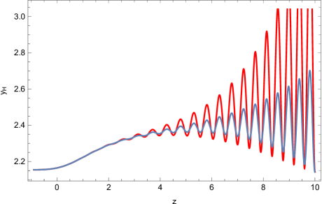
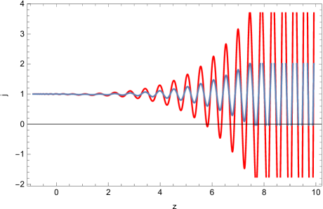
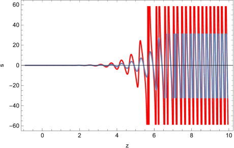
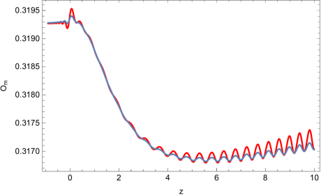
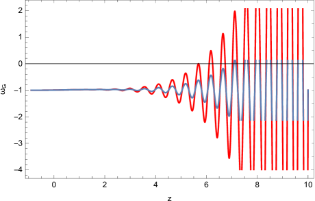
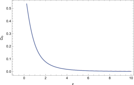
where $z_{f}$ denotes the final redshift $z_{f}=10$. The results of our analysis indicated that the thermal terms effects are significant only for extremely large values of the dimensionless parameter $\alpha$, and specifically for $\alpha\geq 10^{98}$. This can be seen in several statefinder parameters, for example in Fig. 6 we plot the behavior of the statefinder $y_{H}(z)$ as a function of the redshift for the ordinary $f(R)$ gravity (blue curve) and for the thermally corrected $f(R)$ gravity (red curve), for $\alpha=10^{98}$. It is apparent that the dark energy oscillations are more pronounced for large redshifts, for these large $\alpha$ values. The same results are obtained by studying other statefinder quantities, for example in Fig. 7 we present the plots of the deceleration parameter (upper left), the jerk (upper right), the snap (bottom left) and $Om(z)$ (bottom right) as a function of the redshift for the ordinary $f(R)$ gravity (blue curves) and for the thermally corrected $f(R)$ gravity (red curves), for $\alpha=10^{98}$. Finally, differences between the ordinary $f(R)$ gravity (blue curve) and for the thermally corrected $f(R)$ gravity (red curve) can be found by studying the behavior of the dark energy EoS parameter, as it can be seen in Fig. 8. Finally, the only cosmological parameter for which no differences occur between the ordinary $f(R)$ gravity and the thermally corrected $f(R)$ gravity, is the dark energy density parameter $\Omega_{G}$, as it can be seen in Fig. 9.

Figure 9: Plot of the behavior of the dark energy density parameter as a function of the redshift, for the ordinary $f(R)$ gravity (blue curve) and for the thermally corrected $f(R)$ gravity (red curve), for $\alpha=10^{98}$.

In conclusions, the results of our analysis indicate that the ordinary $f(R)$ gravity and the thermally corrected $f(R)$ gravity have differences only when the coefficient $\alpha$ of the thermal corrections takes quite large values, and the differences can be spotted in statefinders only for redshifts $z\geq 5$.

VI Quantitative Discussion on the Results Obtained and Concluding Remarks

In this paper we examined quantitatively the effects of a thermal term $\sim\alpha H^{4}$ in the phase space of $f(R)$ gravity, in the presence or not of perfect matter fluids. In order to perform our quantitative analysis of the phase space, we have formulated the theory as a dynamical system of four variables (vacuum case) with respect to the $e$-foldings number. This system is similar to the one proposed in Ref. Odintsov:2018uaw , where the authors dealt with the plain $f(R)$ theory. Our main difference is that an additional dynamic variable exists representing the effects of the thermal term $\sim\alpha H^{4}$. Our purpose, in comparison to Ref. Odintsov:2018uaw , was to unveil the difference this term may bring up in the phase space behavior of trajectories.

Choosing the Hubble rate such as to mimic the most important cosmological eras, namely the de Sitter (or quasi-de Sitter) accelerating expansion and the matter-dominated and radiation dominated decelerating expansions, we ended up to an autonomous dynamical system that was able to be studied qualitatively. Basically, by focusing on these distinct cosmological eras, we essentially studied the subspaces of the total phase space, corresponding to these cosmological eras. Subsequently, we proceeded by locating the equilibrium points for each of the three cosmological eras, and thoroughly examined their stability properties. Then, we numerically integrated the dynamical system and we plotted the phase space trajectories to validate our results. Notably, the (quasi-)de Sitter phase is dominated by centre manifolds, however they can be isolated and the stability of the equilibria can be addressed by means of the Hartman-Grobman theorem. For the other two cosmological eras, the fixed points were found to be hyperbolic, thus no such problem arose.

While in the (quasi-)de Sitter phase, the system reaches a stable fixed point that is identical to the plain vacuum theory, meaning that the extra thermal term does not play any crucial role during this era. In that case, we reached viable cosmological solutions with,

$$R=12H_{0}^{2}\,,$$ (66)

in the de Sitter case, where $H(t)=H_{0}$, or

$$R=12H_{0}^{2}-24H_{0}H_{1}t+12H_{1}^{2}t^{2}\,,$$ (67)

in the quasi-de Sitter case, where $H(t)=H_{0}-H_{1}t$, while,

$$x_{4}=0\,,$$ (68)

hence, the effect of the thermal fluid term is asymptotically zero for all the stable trajectories.

However, when the Universe is described by either matter- or radiation-dominated eras, the fixed points of the vacuum $f(R)$ theory become unstable and the extra thermal term has non-trivial effects. In other words, the additional thermal term which was added by hand in order to examine these eras, can cause dramatic effects during the classical eras of the standard cosmological model and the viable cosmological solutions are characterized by a non-trivial thermal effects. In this case, for $m=-\dfrac{9}{2}$, meaning that $H(t)=\dfrac{2}{3t}$, we have

$$R=\dfrac{28}{3t^{2}}\,,$$ (69)

and for $m=-8$ and thus $H(t)=\dfrac{1}{2t}$, we have

$$R=\dfrac{6}{t^{2}}\,,$$ (70)

so curvature decreases rapidly over time. As for the additional thermal term, it increases rapidly over time as

$$\alpha H^{4}=\dfrac{27}{2\kappa^{2}}t^{4}\,,$$ (71)

so it becomes more and more important as the viable solution-trajectory in the phase space is attained. Thus clearly, the thermal effects should not be present during the (quasi) de-Sitter, matter and radiation domination eras, as we expected. The effects of the thermal terms though, cause severe instabilities to the dynamical system near a Big Rip singularity, as we expected.

Introducing two typical perfect fluids, relativistic (radiation) and non-relativistic (dust) matter as in the standard cosmological model, the situation does not change. The two further dynamic variables included are rapidly attracted to zero, hence the fixed points of the vacuum theory are basically the same and the above analysis holds true in this case too.

Choosing a different type of Hubble rate, of the type that models the four types of finite-time singularities, we reach a non-autonomous dynamical system, which cannot be analyzed qualitatively in the same manner, mostly due to possessing no invariant sets per se. In this case, we attempted to reduce the system and derive analytical solutions. Indeed, for the case of the “Big Rip” singularity, an analytical solution is obtained that matches the numerical solutions; these cannot asymptotically reach the (quasi-)de Sitter fixed points as the $e$-foldings number tends to infinity, since for any initial value of $N_{c}$, the trajectories are repelled away as the singularity is approached. Thus, as we already mentioned, the dynamical system of $f(R)$ gravity has strong instabilities when it is studied near a Big Rip singularity, as we actually expected.

Moreover, we examined quantitatively the effects of a thermal term of the form $\sim\alpha H^{4}$ on the late-time era, by analyzing several observable quantities related directly to the late-time era. As we showed by using a numerical analysis approach, the ordinary $f(R)$ gravity and the thermally corrected $f(R)$ gravity have differences only when the coefficient $\alpha$ of the thermal corrections takes quite large values, and the differences can be spotted in statefinders only for redshifts $z\geq 5$, where the dark energy oscillations are more pronounced in the thermally corrected $f(R)$ gravity.

Before ending, we need to further clarify some issues. Firstly, the effect of the thermal terms on the matter and radiation domination eras. In theory this term should not have any quantitative role during the matter and radiation domination eras, since there is no horizon related to these eras. So our strategy was to add this term by hand and see, just from curiosity, its effects explicitly. Our results demonstrated that this term, if it was actually present, it would destroy the phase space structure of the matter and radiation domination eras, in the context of $f(R)$ gravity. Thus our analysis showed that indeed, the presence of the thermal radiation term should not be present during the matter and radiation domination eras. Initially we thought that it would not affect at all the dynamical system, but contrary to our expectation, adopting an unquestionable formal and mathematically rigorous approach, this term utterly affects the matter and radiation eras, thus it should not be present during the matter and radiation domination eras at all.

Another issue is related to the interesting question of having finite-time singularities related for example in some subspace of the total phase space, for example in the de Sitter subspace of trajectories. This question was also addressed by us in Ref. Odintsov:2018uaw , but not for $f(R)$ gravity phase space and its subspaces. The finite-time singularity analysis of Ref. Odintsov:2018uaw was focused on perfect fluid-related dynamical systems. But the original question of examining finite-time singularities in the framework of $f(R)$ gravity phase space subspaces, is quite deep in its essence. We believe that the two concepts, namely the finite-time singularities and the fixed points are not necessarily related, at least at the fundamental level of the dynamical systems analysis. In a dynamical system, the phase space and its subspaces are studied, so the presence of a fixed point means that there is attraction, or repulsion for this fixed point. A finite time singularity always leads to blow-ups in the trajectory belonging to the total phase space and in some specific phase space describing a class of trajectories.

But as we mentioned, the above question is deeper and insightful. This question was addressed in Ref. Odintsov:2018uaw for perfect fluid dynamical systems, and to our opinion, it might be possible that a trajectory belonging to a de Sitter, for instance, subspace of the total phase space, might end up to a sudden blow-up values for the parameters that quantify the phase space, if the de Sitter fixed point is unstable for instance. We aim to formally address this issue in a future work.

References

- (1) A. G. Riess et al. [Supernova Search Team], Astron. J. 116 (1998), 1009-1038 doi:10.1086/300499 [arXiv:astro-ph/9805201 [astro-ph]].
- (2) S. Nojiri, S. D. Odintsov and V. K. Oikonomou, Phys. Rept. 692 (2017) 1 doi:10.1016/j.physrep.2017.06.001 [arXiv:1705.11098 [gr-qc]].
- (3) S. Nojiri, S.D. Odintsov, Phys. Rept. 505, 59 (2011);
- (4) S. Nojiri, S.D. Odintsov, eConf C0602061, 06 (2006) [Int. J. Geom. Meth. Mod. Phys. 4, 115 (2007)]. [arXiv:hep-th/0601213];
- (5) S. Capozziello, M. De Laurentis, Phys. Rept. 509, 167 (2011) [arXiv:1108.6266 [gr-qc]]. V. Faraoni and S. Capozziello, Fundam. Theor. Phys. 170 (2010). doi:10.1007/978-94-007-0165-6
- (6) A. de la Cruz-Dombriz and D. Saez-Gomez, Entropy 14 (2012) 1717 doi:10.3390/e14091717 [arXiv:1207.2663 [gr-qc]].
- (7) G. J. Olmo, Int. J. Mod. Phys. D 20 (2011) 413 doi:10.1142/S0218271811018925 [arXiv:1101.3864 [gr-qc]].
- (8) S. D. Odintsov and V. K. Oikonomou, Phys. Rev. D 101 (2020) no.4, 044009 doi:10.1103/PhysRevD.101.044009 [arXiv:2001.06830 [gr-qc]].
- (9) S. Nojiri and S. D. Odintsov, Phys. Rev. D 68 (2003), 123512 doi:10.1103/PhysRevD.68.123512 [arXiv:hep-th/0307288 [hep-th]].
- (10) S. Nojiri and S. D. Odintsov, Phys. Dark Univ. 30 (2020), 100695 doi:10.1016/j.dark.2020.100695 [arXiv:2006.03946 [gr-qc]].
- (11) S. Bahamonde, C. G. Boehmer, S. Carloni, E. J. Copeland, W. Fang and N. Tamanini, Phys. Rept. 775-777 (2018), 1-122 doi:10.1016/j.physrep.2018.09.001 [arXiv:1712.03107 [gr-qc]].
- (12) V. K. Oikonomou and N. Chatzarakis, arXiv:1905.01904 [gr-qc].
- (13) V. K. Oikonomou, arXiv:1907.02600 [gr-qc].
- (14) S. D. Odintsov and V. K. Oikonomou, Phys. Rev. D 98 (2018) no.2, 024013 doi:10.1103/PhysRevD.98.024013 [arXiv:1806.07295 [gr-qc]].
- (15) S. D. Odintsov and V. K. Oikonomou, Phys. Rev. D 97 (2018) no.12, 124042 doi:10.1103/PhysRevD.97.124042 [arXiv:1806.01588 [gr-qc]].
- (16) C. G. Boehmer and N. Chan, doi:10.1142/9781786341044.0004 arXiv:1409.5585 [gr-qc].
- (17) C. G. Boehmer, T. Harko and S. V. Sabau, Adv. Theor. Math. Phys. 16 (2012) no.4, 1145 doi:10.4310/ATMP.2012.v16.n4.a2 [arXiv:1010.5464 [math-ph]].
- (18) N. Goheer, J. A. Leach and P. K. S. Dunsby, Class. Quant. Grav. 24 (2007) 5689 doi:10.1088/0264-9381/24/22/026 [arXiv:0710.0814 [gr-qc]].
- (19) G. Leon and E. N. Saridakis, JCAP 1504 (2015) no.04, 031 doi:10.1088/1475-7516/2015/04/031 [arXiv:1501.00488 [gr-qc]].
- (20) J. Q. Guo and A. V. Frolov, Phys. Rev. D 88 (2013) no.12, 124036 doi:10.1103/PhysRevD.88.124036 [arXiv:1305.7290 [astro-ph.CO]].
- (21) G. Leon and E. N. Saridakis, Class. Quant. Grav. 28 (2011) 065008 doi:10.1088/0264-9381/28/6/065008 [arXiv:1007.3956 [gr-qc]].
- (22) J. C. C. de Souza and V. Faraoni, Class. Quant. Grav. 24 (2007) 3637 doi:10.1088/0264-9381/24/14/006 [arXiv:0706.1223 [gr-qc]].
- (23) A. Giacomini, S. Jamal, G. Leon, A. Paliathanasis and J. Saavedra, Phys. Rev. D 95 (2017) no.12, 124060 doi:10.1103/PhysRevD.95.124060 [arXiv:1703.05860 [gr-qc]].
- (24) G. Kofinas, G. Leon and E. N. Saridakis, Class. Quant. Grav. 31 (2014) 175011 doi:10.1088/0264-9381/31/17/175011 [arXiv:1404.7100 [gr-qc]].
- (25) G. Leon and E. N. Saridakis, JCAP 1303 (2013) 025 doi:10.1088/1475-7516/2013/03/025 [arXiv:1211.3088 [astro-ph.CO]].
- (26) T. Gonzalez, G. Leon and I. Quiros, Class. Quant. Grav. 23 (2006) 3165 doi:10.1088/0264-9381/23/9/025 [astro-ph/0702227].
- (27) A. Alho, S. Carloni and C. Uggla, JCAP 1608 (2016) no.08, 064 doi:10.1088/1475-7516/2016/08/064 [arXiv:1607.05715 [gr-qc]].
- (28) S. K. Biswas and S. Chakraborty, Int. J. Mod. Phys. D 24 (2015) no.07, 1550046 doi:10.1142/S0218271815500467 [arXiv:1504.02431 [gr-qc]].
- (29) D. Muller, V. C. de Andrade, C. Maia, M. J. Reboucas and A. F. F. Teixeira, Eur. Phys. J. C 75 (2015) no.1, 13 doi:10.1140/epjc/s10052-014-3227-2 [arXiv:1405.0768 [astro-ph.CO]].
- (30) B. Mirza and F. Oboudiat, Int. J. Geom. Meth. Mod. Phys. 13 (2016) no.09, 1650108 doi:10.1142/S0219887816501085 [arXiv:1412.6640 [gr-qc]].
- (31) S. Rippl, H. van Elst, R. K. Tavakol and D. Taylor, Gen. Rel. Grav. 28 (1996) 193 doi:10.1007/BF02105423 [gr-qc/9511010].
- (32) M. M. Ivanov and A. V. Toporensky, Grav. Cosmol. 18 (2012) 43 doi:10.1134/S0202289312010100 [arXiv:1106.5179 [gr-qc]].
- (33) M. Khurshudyan, Int. J. Geom. Meth. Mod. Phys. 14 (2016) no.03, 1750041. doi:10.1142/S0219887817500414
- (34) R. D. Boko, M. J. S. Houndjo and J. Tossa, Int. J. Mod. Phys. D 25 (2016) no.10, 1650098 doi:10.1142/S021827181650098X [arXiv:1605.03404 [gr-qc]].
- (35) S. D. Odintsov, V. K. Oikonomou and P. V. Tretyakov, Phys. Rev. D 96 (2017) no.4, 044022 doi:10.1103/PhysRevD.96.044022 [arXiv:1707.08661 [gr-qc]].
- (36) L. N. Granda and D. F. Jimenez, arXiv:1710.07273 [gr-qc].
- (37) F. F. Bernardi and R. G. Landim, Eur. Phys. J. C 77 (2017) no.5, 290 doi:10.1140/epjc/s10052-017-4858-x [arXiv:1607.03506 [gr-qc]].
- (38) R. C. G. Landim, Eur. Phys. J. C 76 (2016) no.1, 31 doi:10.1140/epjc/s10052-016-3894-2 [arXiv:1507.00902 [gr-qc]].
- (39) R. C. G. Landim, Eur. Phys. J. C 76 (2016) no.9, 480 doi:10.1140/epjc/s10052-016-4328-x [arXiv:1605.03550 [hep-th]].
- (40) P. Bari, K. Bhattacharya and S. Chakraborty, arXiv:1805.06673 [gr-qc].
- (41) M. G. Ganiou, P. H. Logbo, M. J. S. Houndjo and J. Tossa, arXiv:1805.00332 [gr-qc].
- (42) P. Shah, G. C. Samanta and S. Capozziello, arXiv:1803.09247 [gr-qc].
- (43) V. K. Oikonomou, Int. J. Mod. Phys. D 27 (2018) no.05, 1850059 doi:10.1142/S0218271818500591 [arXiv:1711.03389 [gr-qc]].
- (44) S. D. Odintsov and V. K. Oikonomou, Phys. Rev. D 96 (2017) no.10, 104049 doi:10.1103/PhysRevD.96.104049 [arXiv:1711.02230 [gr-qc]].
- (45) J. Dutta, W. Khyllep, E. N. Saridakis, N. Tamanini and S. Vagnozzi, JCAP 1802 (2018) 041 doi:10.1088/1475-7516/2018/02/041 [arXiv:1711.07290 [gr-qc]].
- (46) S. D. Odintsov and V. K. Oikonomou, Phys. Rev. D 93 (2016) no.2, 023517 doi:10.1103/PhysRevD.93.023517 [arXiv:1511.04559 [gr-qc]].
- (47) K. Kleidis and V. K. Oikonomou, arXiv:1808.04674 [gr-qc].
- (48) V. K. Oikonomou, Phys. Rev. D 99 (2019) no.10, 104042 doi:10.1103/PhysRevD.99.104042 [arXiv:1905.00826 [gr-qc]].
- (49) N. Chatzarakis and V. K. Oikonomou, Annals Phys. 419 (2020), 168216 doi:10.1016/j.aop.2020.168216 [arXiv:1908.08141 [gr-qc]].
- (50) S. Nojiri, S. D. Odintsov and S. Tsujikawa, Phys. Rev. D 71 (2005), 063004 doi:10.1103/PhysRevD.71.063004 [arXiv:hep-th/0501025 [hep-th]].
- (51) S. D. Odintsov, V. K. Oikonomou and F. P. Fronimos, Phys. Dark Univ. 29 (2020), 100563 doi:10.1016/j.dark.2020.100563 [arXiv:2004.08884 [gr-qc]].
- (52) N. Aghanim et al. [Planck], [arXiv:1807.06209 [astro-ph.CO]].
- (53) K. Bamba, A. Lopez-Revelles, R. Myrzakulov, S. D. Odintsov and L. Sebastiani, Class. Quant. Grav. 30 (2013), 015008 doi:10.1088/0264-9381/30/1/015008 [arXiv:1207.1009 [gr-qc]].