1 Introduction

Supersymmetry (Susy) is one of the prime candidates for physics Beyond the Standard Model (BSM). A particularly well motivated Susy model is the so-called $\mu$-from-$\nu$ Supersymmetric Standard Model ($\mu\nu$SSM) [1, 2]. Beyond the usual benefits of low-scale Susy, i.e., providing a solution to the hierarchy problem and allowing for the unification of the three Standard Model (SM) gauge couplings, the $\mu\nu$SSM incorporates an electroweak seesaw mechanism. Without introducing any scales beyond the Susy-breaking scale $M_{S}$, the tiny neutrino masses and their mixing pattern can be accommodated assuming neutrino Yukawa couplings $Y^{\nu}$ of the order of the electron Yukawa coupling. Furthermore, the superpotential is scale invariant and the $\mu$-term of the superpotential of the Minimal Supersymmetric Standard Model (MSSM) is generated dynamically during Electroweak Symmetry Breaking (EWSB). Apart from the Higgs doublets, also the scalar partners of the neutrinos (called sneutrinos) obtain a Vacuum Expectation Value (vev) during EWSB. The tree-level mass of the SM-like Higgs boson receives additional contributions stemming from portal couplings between the Higgs doublet fields and the right-handed sneutrinos. Thus, compared to the MSSM, a value of $\sim 125\ \mathrm{GeV}$ can be achieved with fewer radiative corrections.

The $\mu\nu$SSM is especially interesting in view of EWSB. In this model the stability of the proton is assured by forbidding operators breaking baryon number [2]. However, it does not assume $R$-parity conservation and the breaking of lepton number is induced via terms proportional to $Y^{\nu}$ by construction. Thus, the left- and right-handed sneutrinos mix with the neutral scalar components of the Higgs doublet superfields. Apart from that, the scalar partners of the leptons (called sleptons) mix with the charged scalar components of the Higgs doublet superfields. Neglecting CP violation, as we will do throughout this paper, the Higgs sector of the $\mu\nu$SSM consists of a total of 8 CP-even, 7 CP-odd, and ${2\times 7}$ charged scalars. In addition, there are the usual pseudoscalar and charged Goldstone bosons $G^{0}$ and $G^{\pm}$. During EWSB all of the 8 neutral scalar fields obtain a vev. While the mixing of the doublet Higgs bosons and the gauge-singlet right-handed sneutrinos can in principle be arbitrarily large, the mixing between the left-handed sneutrinos and the Higgs doublets is suppressed by the small values of $Y^{\nu}$. This decoupling is also reflected in a large hierarchy between the vevs. The vevs of the Higgs doublets $v_{u}$ and $v_{d}$ and the vevs of the right-handed sneutrinos $v_{iR}$ ($i=1,2,3$) are related to the breaking scale of the EW symmetry and Susy. The vevs of the left-handed sneutrinos $v_{iL}$, on the other hand, are related to the breaking of lepton number, and therefore suppressed by a factor of $Y^{\nu}$ compared to $v_{d}$, $v_{u}$ and $v_{iR}$.

These unique features motivated the precise analysis of the Higgs sector of the model, including the radiative corrections at full one-loop level. At first, we studied a simplified version of the $\mu\nu$SSM with a single right-handed neutrino superfield [3]. Later on, we extended the calculation to the complete model with three right-handed neutrino superfields [4]. In the latter, three non-zero left-handed neutrino masses can already be accommodated at tree level. It was found that for the SM-like Higgs-boson mass the mixing effects between doublet fields and right-handed sneutrinos are important at loop level and have to be taken into account, while the tiny mixing with the left-handed sneutrinos does not play a role. However, the left-handed sneutrinos themselves are subject to potentially large corrections proportional to $Y^{\nu}A_{t}Y_{t}/v_{iL}$, in which the suppression of the factors $Y^{\nu}$ is compensated by the left-handed vevs in the denominator and a factor of the soft scalar top (called stop) mixing parameter $A_{t}$ times the top Yukawa coupling $Y_{t}$.

It is known from the MSSM that corrections to the Higgs-boson mass beyond one-loop level are sizable and have to be taken into account [5, 6, 7]. These higher-order contributions should be included in an approximate form also in the $\mu\nu$SSM in order to obtain an accurate prediction. Combining the higher-order effects with the full one-loop result, it was shown that the $\mu\nu$SSM can easily accommodate a Higgs boson at $\sim 125\ \mathrm{GeV}$ that reproduces the measured signal rates within the current experimental uncertainties [4]. Apart from that, interesting new Higgs physics can be realized at relatively low masses, since the right- and the left-handed sneutrinos could have escaped discovery so far even for masses below $125\ \mathrm{GeV}$ [4]. Note that the right-handed sneutrinos are gauge singlets, such that they naturally have reduced couplings to the SM particles. In fact, they only couple to the SM via the mixing with the doublet fields, for instance the SM-like Higgs boson. Such a scenario is particularly interesting, as it can be probed not only by directly searching for additional Higgs bosons, but also indirectly by measuring possible deviations from the SM predictions of the couplings of the Higgs boson at $125\ \mathrm{GeV}$ [4, 8]. A possible detection of light left-handed sneutrinos requires dedicated searches when they are the lightest Susy particle, since their decay must proceed via $R$-parity violating couplings [9, 10, 11].

In this paper we present the tool munuSSM for the phenomenological study of the $\mu\nu$SSM. In contrast to the already existing public codes SARAH/SPheno [12, 13, 14, 15, 16, 17] and FlexibleSUSY [18, 19, 20], which are designed to be generically applicable to various different (Susy) extensions of the SM, the code munuSSM is targeted specifically at the $\mu\nu$SSM. First and foremost, it makes the one-loop corrections to the Higgs potential publicly available in terms of the momentum-dependent renormalized scalar self energies. These are used in combination with leading higher-order corrections from the public code FeynHiggs [21, 7, 22, 23, 24, 25, 26, 27] to accurately predict the particle masses of the neutral scalars, in particular the SM-like Higgs-boson mass. In addition, the radiative corrections to the mixing matrix elements are used to obtain effective couplings of the scalars to the SM particles. Furthermore, the calculation of the branching ratios of the neutral and charged scalars is implemented. For decays into SM particles, the branching ratios are obtained by rescaling the SM predictions [28, 29] by the effective couplings. For decays to BSM final states, the branching ratios are calculated from scratch at leading order, however including radiative corrections by rotating the tree-level couplings into the loop-corrected mass eigenstate basis. The effective couplings and branching ratios can be directly interfaced to the public codes HiggsBounds [30, 31, 32, 33, 34, 35] and HiggsSignals [36, 37, 38, 39] to test a benchmark point against collider constraints. The interface to HiggsBounds also provides the LHC cross sections normalized to the SM prediction, which are extracted from the effective couplings.

The paper is organized as follows. We start by briefly introducing the model in Sect. 2. The overall structure of the code munuSSM and its subpackages are described in Sect. 3, paying special attention to the links to other public codes in Sect. 3.1. Afterwards, we explain the installation process and the basic user instructions in Sect. 3.2 and Sect. 3.3. A simple example analysis is described in Sect. 4. We conclude in Sect. 5.

2 The $\mu$-from-$\nu$ Supersymmetric Standard Model

In this section we provide the basic definitions and conventions under which the model predictions were implemented. A more detailed motivation and a review of the $\mu\nu$SSM can be found in Ref. [40]. The calculation of the radiative corrections to the Higgs potential are described in detail in Refs. [3, 4].

The superpotential of the $\mu\nu$SSM is written as

$$W=\; \epsilon_{ab}\left(Y^{e}_{ij}\,\hat{H}_{d}^{a}\,\hat{L}^{b}_{i}\,\hat{e}_{j}^{c}+Y^{d}_{ij}\,\hat{H}_{d}^{a}\,\hat{Q}^{b}_{i}\,\hat{d}_{j}^{c}+Y^{u}_{ij}\,\hat{H}_{u}^{b}\,\hat{Q}^{a}_{i}\,\hat{u}_{j}^{c}\right)$$

$$+\; \epsilon_{ab}\left(Y^{\nu}_{ij}\,\hat{H}_{u}^{b}\,\hat{L}^{a}_{i}\,\hat{\nu}^{c}_{j}-\lambda_{i}\,\hat{\nu}^{c}_{i}\,\hat{H}_{u}^{b}\hat{H}_{d}^{a}\right)+\frac{1}{3}\kappa{{}_{ijk}}\hat{\nu}^{c}_{i}\hat{\nu}^{c}_{j}\hat{\nu}^{c}_{k}\ ,$$ (1)

where $\hat{H}_{d}^{T}=(\hat{H}_{d}^{0},\hat{H}_{d}^{-})$ and $\hat{H}_{u}^{T}=(\hat{H}_{u}^{+},\hat{H}_{u}^{0})$ are the Higgs doublet superfields, $\hat{Q}_{i}^{T}=(\hat{u}_{i},\hat{d}_{i})$ and $\hat{L}_{i}^{T}=(\hat{\nu}_{i},\hat{e}_{i})$ are the left-chiral quark and lepton superfields, and $\hat{u}_{j}^{c}$, $\hat{d}_{j}^{c}$, $\hat{e}_{j}^{c}$ and $\hat{\nu}^{c}$ are the right-chiral quark and lepton superfields. $i,j=1,2,3$ are the family indices, and $a,b=1,2$ are indices of the fundamental representation of SU(2) with $\epsilon_{ab}=1$. The colour indices are not written out.

In the framework of low-energy Susy breaking, the soft Lagrangian of the $\mu\nu$SSM is given by [41]

$$-\mathcal{L}_{\text{soft}} =\;\epsilon_{ab}\left(T^{e}_{ij}\,H_{d}^{a}\,\widetilde{L}^{b}_{iL}\,\widetilde{e}_{jR}^{*}+T^{d}_{ij}\,H_{d}^{a}\,\widetilde{Q}^{b}_{iL}\,\widetilde{d}_{jR}^{*}+T^{u}_{ij}\,H_{u}^{b}\widetilde{Q}^{a}_{iL}\widetilde{u}_{jR}^{*}+\text{h.c.}\right)$$

$$+\; \epsilon_{ab}\left(T^{\nu}_{ij}\,H_{u}^{b}\,\widetilde{L}^{a}_{iL}\widetilde{\nu}_{jR}^{*}-T^{\lambda}_{i}\,\widetilde{\nu}_{iR}^{*}\,H_{d}^{a}H_{u}^{b}+\frac{1}{3}T^{\kappa}_{ijk}\,\widetilde{\nu}_{iR}^{*}\widetilde{\nu}_{jR}^{*}\widetilde{\nu}_{kR}^{*}\ +\text{h.c.}\right)$$

$$+\; \left(m_{\widetilde{Q}}^{2}\right)_{ij}\widetilde{Q}_{iL}^{a*}\widetilde{Q}^{a}_{jL}+\left(m_{\widetilde{u}}^{2}\right)_{ij}\widetilde{u}_{iR}^{*}\widetilde{u}_{jR}+\left(m_{\widetilde{d}}^{2}\right)_{ij}\widetilde{d}_{iR}^{*}\widetilde{d}_{jR}+\left(m_{\widetilde{L}}^{2}\right)_{ij}\widetilde{L}_{iL}^{a*}\widetilde{L}^{a}_{jL}$$

$$+\; \left(m_{\widetilde{\nu}}^{2}\right)_{ij}\widetilde{\nu}_{iR}^{*}\widetilde{\nu}_{jR}+\left(m_{\widetilde{e}}^{2}\right)_{ij}\widetilde{e}_{iR}^{*}\widetilde{e}_{jR}+m_{H_{d}}^{2}{H^{a}_{d}}^{*}H^{a}_{d}+m_{H_{u}}^{2}{H^{a}_{u}}^{*}H^{a}_{u}$$ (2)

$$+\; \left(\left(m_{H_{d}\widetilde{L}}^{2}\right)_{i}H_{d}^{a*}\widetilde{L}_{iL}^{a}+\text{h.c.}\right)$$

$$+\; \frac{1}{2}\,\left(M_{3}\,{\widetilde{g}}\,{\widetilde{g}}+M_{2}\,{\widetilde{W}}\,{\widetilde{W}}+M_{1}\,{\widetilde{B}}^{0}\,{\widetilde{B}}^{0}+\text{h.c.}\right)\ .$$ (3)

The parameters $m_{H_{d}\widetilde{L}}^{2}$ are absent at tree level, as they are non-diagonal in field space. However, in the code the terms are taken into account, because they are required for the renormalization of the Higgs potential (see Refs. [3, 4] for details). In addition, flavour mixing is neglected in the quark and the squark sector, such that the corresponding soft mass parameters only have diagonal non-zero entries $m_{\widetilde{Q}_{i}}^{2}$, $m_{\widetilde{u}_{i}}^{2}$ and $m_{\widetilde{d}_{i}}^{2}$. The soft trilinear couplings are written as $T^{u}_{i}=A^{u}_{i}Y^{u}_{i}$, $T^{d}_{i}=A^{d}_{i}Y^{d}_{i}$, where $Y^{u}_{i}$ and $Y^{d}_{i}$ are the diagonal entries of the Yukawa couplings of the up- and down-type quarks and no summation over repeated indices is implied. In the lepton sector, the flavour symmetries are broken automatically after EWSB. Thus, we decompose the soft trilinear couplings as $T^{e}_{ij}=A^{e}_{ij}Y^{e}_{ij}$ and $T^{\nu}_{ij}=A^{\nu}_{ij}Y^{\nu}_{ij}$, again without summation over repeated indices. The lepton-flavour mixing is suppressed by factors of $Y^{\nu}_{ij}$ and therefore only sizable for the light left-handed neutrinos. Finally, we write the portal coupling and the self coupling of the right-handed sneutrinos as $T^{\lambda}_{i}=A^{\lambda}_{i}\lambda_{i}$ and $T^{\kappa}_{ijk}=A^{\kappa}_{ijk}\kappa_{ijk}$, noting that both $\kappa_{ijk}$ and $A^{\kappa}_{ijk}$ are symmetric under the exchange of indices.

The soft terms together with the $D$-term and $F$-term contributions from the superpotential define the tree-level neutral scalar potential

$$V^{(0)}=V_{\text{soft}}+V_{F}+V_{D}\ ,$$ (4)

with

$$V_{\text{soft}}=\; \left(T^{\nu}_{ij}\,H_{u}^{0}\,\widetilde{\nu}_{iL}\,\widetilde{\nu}_{jR}^{*}-T^{\lambda}_{i}\,\widetilde{\nu}_{iR}^{*}\,H_{d}^{0}H_{u}^{0}+\frac{1}{3}T^{\kappa}_{ijk}\,\widetilde{\nu}_{iR}^{*}\widetilde{\nu}_{jR}^{*}\widetilde{\nu}_{kR}^{*}\ +\text{h.c.}\right)$$

$$+\; \left(m_{\widetilde{L}}^{2}\right)_{ij}\widetilde{\nu}_{iL}^{*}\widetilde{\nu}_{jL}+\left(m_{\widetilde{\nu}}^{2}\right)_{ij}\widetilde{\nu}_{iR}^{*}\widetilde{\nu}_{jR}+m_{H_{d}}^{2}{H^{0}_{d}}^{*}H^{0}_{d}+m_{H_{u}}^{2}{H^{0}_{u}}^{*}H^{0}_{u}\ ,$$ (5)

$$V_{F}=\; \lambda_{j}\lambda_{j}H^{0}_{d}H_{d}^{0}{{}^{{}^{*}}}H^{0}_{u}H_{u}^{0}{{}^{{}^{*}}}+\lambda_{i}\lambda_{j}\tilde{\nu}^{*}_{iR}\tilde{\nu}_{jR}H^{0}_{d}H_{d}^{0}{{}^{*}}+\lambda_{i}\lambda_{j}\tilde{\nu}^{*}_{iR}\tilde{\nu}_{jR}H^{0}_{u}H_{u}^{0}{{}^{*}}$$

$$+\; \kappa_{ijk}\kappa_{ljm}\tilde{\nu}^{*}_{iR}\tilde{\nu}_{lR}\tilde{\nu}^{*}_{kR}\tilde{\nu}_{mR}-\left(\kappa_{ijk}\lambda_{j}\tilde{\nu}^{*}_{iR}\tilde{\nu}^{*}_{kR}H_{d}^{0*}H_{u}^{0*}-Y^{\nu}_{ij}\kappa_{ljk}\tilde{\nu}_{iL}\tilde{\nu}_{lR}\tilde{\nu}_{kR}H^{0}_{u}\right.$$

$$+\; \left.Y^{\nu}_{ij}\lambda_{j}\tilde{\nu}_{iL}H_{d}^{0*}H_{u}^{0*}H^{0}_{u}+{Y^{\nu}_{ij}}\lambda_{k}\tilde{\nu}_{iL}^{*}\tilde{\nu}_{jR}\tilde{\nu}_{kR}^{*}H^{0}_{d}+\text{h.c.}\right)$$

$$+\; Y^{\nu}_{ij}{Y^{\nu}_{ik}}\tilde{\nu}^{*}_{jR}\tilde{\nu}_{kR}H^{0}_{u}H_{u}^{0}{{}^{*}}+Y^{\nu}_{ij}{Y^{\nu}_{lk}}\tilde{\nu}_{iL}\tilde{\nu}_{lL}^{*}\tilde{\nu}_{jR}^{*}\tilde{\nu}_{kR}+Y^{\nu}_{ji}{Y^{\nu}_{ki}}\tilde{\nu}_{jL}\tilde{\nu}_{kL}^{*}H^{0}_{u}H_{u}^{0*}\,,$$ (6)

$$V_{D}=\; \frac{1}{8}\left(g_{1}^{2}+g_{2}^{2}\right)\left(\widetilde{\nu}_{iL}\widetilde{\nu}_{iL}^{*}+H^{0}_{d}{H^{0}_{d}}^{*}-H^{0}_{u}{H^{0}_{u}}^{*}\right)^{2}\,.$$ (7)

During EWSB the neutral scalar fields acquire a vev. We use the decomposition

$$H_{d}^{0} =\frac{1}{\sqrt{2}}\left(H_{d}^{\mathcal{R}}+v_{d}+\text{i}\,H_{d}^{\mathcal{I}}\right)\ ,$$ (8)

$$H^{0}_{u} =\frac{1}{\sqrt{2}}\left(H_{u}^{\mathcal{R}}+v_{u}+\text{i}\,H_{u}^{\mathcal{I}}\right)\ ,$$ (9)

$$\widetilde{\nu}_{iR} =\frac{1}{\sqrt{2}}\left(\widetilde{\nu}^{\mathcal{R}}_{iR}+v_{iR}+\text{i}\,\widetilde{\nu}^{\mathcal{I}}_{iR}\right)\ ,$$ (10)

$$\widetilde{\nu}_{iL} =\frac{1}{\sqrt{2}}\left(\widetilde{\nu}_{iL}^{\mathcal{R}}+v_{iL}+\text{i}\,\widetilde{\nu}_{iL}^{\mathcal{I}}\right)\ ,$$ (11)

such that the vevs are given by

$$\langle H_{d}^{0}\rangle=\frac{v_{d}}{\sqrt{2}}\ ,\,\quad\langle H_{u}^{0}\rangle=\frac{v_{u}}{\sqrt{2}}\ ,\,\quad\langle\widetilde{\nu}_{iR}\rangle=\frac{v_{iR}}{\sqrt{2}}\ ,\,\quad\langle\widetilde{\nu}_{iL}\rangle=\frac{v_{iL}}{\sqrt{2}}\;.$$ (12)

The subscripts ^R and ^I denote CP-even and -odd components of each scalar field, respectively. To make a connection to the SM and the MSSM, we define the parameters

$$v^{2}=v_{u}^{2}+v_{d}^{2}+v_{iL}v_{iL}\sim 246\ \mathrm{GeV}\quad\text{and}\quad\tan\beta=\frac{v_{u}}{v_{d}}\ .$$ (13)

As already mentioned in Sect. 1, the size of the left-handed vevs $v_{iL}$ is suppressed by factors of $Y^{\nu}_{ij}$ compared to the other vevs. Hence, they are of the order of $\sim 10^{-5}$ to $10^{-4}\ \mathrm{GeV}$. The minimization or tadpole equations relate the soft mass parameters to the vevs. For numerical reasons it is most convenient to use the vevs as input parameters and solve the tadpole equations for the soft masses squared $m_{H_{d}}^{2}$, $m_{H_{u}}^{2}$, $(m_{\widetilde{L}}^{2})_{ii}$ and $(m_{\widetilde{\nu}}^{2})_{ii}$. The precise form of the tadpole equations can be found in Ref. [4].

The expressions for the tree-level masses of all particles of the model in terms of the parameters defined above can be found in Ref. [42]. Since they are rather lengthy we do not repeat them here. The expressions for the tree-level couplings of the particles are even larger due to the complicated mixing in the scalar sector, such that we do not state them either. Instead, we provide a FeynArts [43] modelfile upon request that contains the couplings in the ’t Hooft-Feynman gauge in Mathematica syntax. The modelfile was initially created with the public tool SARAH [17], but further modified by hand to allow the usage of the tool FormCalc [46], which by default cannot process the huge expressions for the couplings produced by SARAH.

In the code munuSSM, the calculation of the tree-level spectrum and the corresponding mixing matrices, as well as the tree-level couplings, are evaluated in Fortran subroutines. This allows for a larger floating-point precision, which is necessary due to the tiny $R$-parity violating mixing effects and the large hierarchy between the masses in the neutral fermion sector. Apart from that, the usage of Fortran vastly improves the running time compared to an implementation in python. We note that the running time is currently dominated by the calculation of the complete set of tree-level couplings.

2.1 Radiative corrections in the Higgs sector

The scalar sector of the $\mu\nu$SSM is subject to sizable radiative corrections that have to be taken into account in each phenomenologically viable analysis. Making these corrections available to the public is (so far) the core idea of this project. The objects that contain the corrections are the renormalized scalar self energies $\hat{\Sigma}_{\phi_{i}\phi_{j}}(p^{2})$, which enter the renormalized inverse propagator matrix of the fields $\phi_{i}$,

$$\hat{\Gamma}_{ij}=\text{i}\left[\delta_{ij}(p^{2}-m_{i}^{2})-\hat{\Sigma}_{\phi_{i}\phi_{j}}(p^{2})\right]\ .$$ (14)

In this expression the indices $i$ and $j$ run over the number of fields that mix with each other, $p$ is the momentum and $m_{i}^{2}$ are the eigenvalues of the corresponding tree-level mass matrix. Implemented in the code are the corrections to the CP-even and CP-odd neutral scalars $h_{i}$ and $A_{i}$. These are given by

$$\hat{\Sigma}_{h_{i}h_{j}} =\hat{\Sigma}_{h_{i}h_{j}}^{(1)}(p^{2})+\hat{\Sigma}_{h_{i}h_{j}}^{(2^{\prime})}+\hat{\Sigma}_{h_{i}h_{j}}^{\mathrm{resum.}}$$ (15)

$$\hat{\Sigma}_{A_{i}A_{j}} =\hat{\Sigma}_{A_{i}A_{j}}^{(1)}(p^{2})\ .$$ (16)

Here, $\hat{\Sigma}_{h_{i}h_{j}}^{(1)}$ and $\hat{\Sigma}_{A_{i}A_{j}}^{(1)}$ contain the full one-loop corrections, including the momentum dependence. In addition, leading two-loop corrections for the CP-even fields $h_{i}$ are included in terms of $\hat{\Sigma}_{h_{i}h_{j}}^{(2^{\prime})}$. Finally, higher-order corrections arising from the resummation of logarithmic contributions are taken into account in $\hat{\Sigma}_{h_{i}h_{j}}^{\mathrm{resum.}}$. The corrections beyond one-loop level are taken from the public code FeynHiggs. They are crucial to obtain a precise prediction for the SM-like Higgs-boson mass. $\hat{\Sigma}_{h_{i}h_{j}}^{(2^{\prime})}$ contains the fixed-order corrections of $\mathcal{O}(\alpha_{t}\alpha_{s},\alpha_{b}\alpha_{s},\alpha_{t}^{2},\alpha_{t}\alpha_{b},\alpha_{b}^{2})$ in the approximation of vanishing electroweak gauge couplings and ${p^{2}=0}$. $\hat{\Sigma}_{h_{i}h_{j}}^{\mathrm{resum.}}$ contains terms from the full resummation of leading and next-to-leading logarithms and next-to-next-to-leading logarithms of $\mathcal{O}(\alpha_{s}\alpha_{t})$, obtained from an effective theory calculation [27].

The one-loop pieces were calculated in Ref. [4] in a mixed $\smash{\overline{\mathrm{DR}}}$-On Shell (OS) scheme that is consistent with the one of FeynHiggs. For generic scalar fields $\phi_{i}$, they can be written as

$$\hat{\Sigma}_{\phi_{i}\phi_{j}}^{(1)}(p^{2}) =\Sigma_{\phi_{i}\phi_{j}}^{(1)}(p^{2})+\frac{1}{2}p^{2}\left(\delta Z_{\phi_{j}\phi_{i}}+\delta Z_{\phi_{i}\phi_{j}}\right)$$

$$-\frac{1}{2}\left(m_{\phi_{k}\phi_{j}}^{2}\delta Z_{\phi_{k}\phi_{i}}+m_{\phi_{i}\phi_{k}}^{2}\delta Z_{\phi_{k}\phi_{j}}\right)-\delta m_{\phi_{i}\phi_{j}}^{2}\ .$$ (17)

$\Sigma_{\phi_{i}\phi_{j}}^{(1)}$ denotes the unrenormalized self energies, extracted from the one-particle irreducible scalar two-point functions. The field-renormalization counterterms $\delta Z_{\phi_{j}\phi_{i}}$ and the mass counterterms $\delta m_{\phi_{i}\phi_{j}}^{2}$ are defined in a way to cancel all ultraviolet divergences appearing in $\Sigma_{\phi_{i}\phi_{j}}^{(1)}$. The finite pieces of the counterterms are defined by the chosen renormalization scheme. The field-renormalization constants are defined as $\smash{\overline{\mathrm{DR}}}$ parameters, such that they do not contain finite terms. The mass counterterms, on the other hand, are defined in a mixed OS-$\smash{\overline{\mathrm{DR}}}$ scheme. The gauge-boson masses $M_{W}$ and $M_{Z}$ and the tadpole coefficients are renormalized applying OS conditions, such that $\delta m_{\phi_{i}\phi_{j}}^{2}$ contains finite contributions from the corresponding counterterms [4].

Without going into too much detail, we summarize the numerical impact of the radiative corrections on the Higgs-boson masses of the $\mu\nu$SSM in the following. Schematically, a rough approximation of the SM-like Higgs-boson mass is given by

$$m_{h^{\rm SM}}^{2}\sim M_{Z}^{2}\cos^{2}(2\beta)+\frac{1}{2}\lambda_{i}\lambda_{i}v^{2}\sin^{2}(2\beta)+\Delta^{\rm MSSM}_{\rm(s)top}+\Delta^{\widetilde{\nu}_{iR}^{\mathcal{R}}}_{\lambda_{i}^{2}}\ ,$$ (18)

where the second term provides the enhancement of the tree-level contribution compared to the MSSM mentioned in Sect. 1. The third term consists of the usual MSSM-like corrections from the stop and the top sector (see Ref. [47] for a review). In the gauge basis, these terms are practically unchanged in the $\mu\nu$SSM. However, the mixing with the right-handed sneutrinos modifies how much of $\Delta^{\rm MSSM}_{\rm(s)top}$ is finally attributed to the mass eigenstate of the SM-like Higgs boson. The last term mainly arises from the mixing of the doublet fields with the right-handed sneutrinos. It was already observed in the next-to MSSM (NMSSM) that, in contrast to the tree-level term dependent on $\lambda_{i}$, the loop-corrections contained in $\Delta^{\widetilde{\nu}_{iR}^{\mathcal{R}}}_{\lambda_{i}^{2}}$ are usually negative and can, depending on the size of the mixing, the value of $\tan\beta$ and the self couplings $\kappa_{ijk}$, substantially decrease the prediction for the SM Higgs-boson mass [48]. Due to the presence of three gauge singlet scalars in the $\mu\nu$SSM instead of only one in the NMSSM, the analytic form of $\Delta^{\widetilde{\nu}_{iR}^{\mathcal{R}}}_{\lambda_{i}^{2}}$ is much more complicated. However, the numerical analysis of such corrections has shown that it is crucial to take into account independently the contributions from all three right-handed sneutrino for a precise prediction of the SM-like Higgs-boson mass [42].

The radiative corrections to the right-handed sneutrinos themselves are sizable only for small masses in the vicinity of $125\ \mathrm{GeV}$ or below [3, 4]. Otherwise, the tree-level mass is already a good estimate. This is due to the fact that the right-handed sneutrinos are gauge singlets and only couple to the SM particle content via a mixing with the Higgs doublet fields. If such mixing exists, the corresponding right-handed sneutrino acquires additional contributions to its mass from $\Delta^{\rm MSSM}_{\rm(s)top}$.

Finally, the most interesting radiative corrections are the ones obtained by the left-handed sneutrinos. They are caused by genuine effects of the $\mu\nu$SSM without a correspondence in the (N)MSSM. It was shown that the dominant contributions arise from the counterterms of the tadpoles, which enter the mass counterterm in Eq. (17) with an inverse factor of the vev of the scalar field under consideration [3]. For the left-handed sneutrinos this means that they are enhanced by the inverse of the small values of $v_{iL}$. This enhancement can compensate the suppression of factors of $Y^{\nu}_{ij}$ present in lepton-number violating couplings. Here, the corrections are mainly given by the tadpole diagrams with the stops in the loop. The stops are coupled to the left-handed sneutrinos via an $F$-term tree-level coupling between $\widetilde{t}_{L}$, $\widetilde{t}_{R}$, $\widetilde{\nu}_{iL}$ and $\widetilde{\nu}_{iR}$, after replacing $\widetilde{\nu}_{iR}$ with the corresponding vev $v_{iR}$. Expanding the complete renormalized self energy in powers of $A^{u}_{3}=A_{t}$ and $1/v_{iL}$, one finds the very good approximation

$$\hat{\Sigma}_{\widetilde{\nu}_{iL}^{\mathcal{R}}\widetilde{\nu}_{iL}^{\mathcal{R}}}^{(1)} \approx\left.\hat{\Sigma}_{\widetilde{\nu}_{iL}^{\mathcal{R}}\widetilde{\nu}_{iL}^{\mathcal{R}}}^{(1)}\right|_{\frac{A_{t}}{v_{iL}}}=$$

$$\frac{3}{16\pi^{2}}\frac{v_{u}v_{iR}}{\sqrt{2}v_{iL}}A_{t}Y_{t}^{2}Y^{\nu}_{ii}\left(\frac{\log{(\frac{m_{\widetilde{t}_{1}}^{2}}{\mu_{R}^{2}})}m_{\widetilde{t}_{1}}^{2}-\log{(\frac{m_{\widetilde{t}_{2}}^{2}}{\mu_{R}^{2}})}m_{\widetilde{t}_{2}}^{2}}{m_{\widetilde{t}_{1}}^{2}-m_{\widetilde{t}_{2}}^{2}}-1\right)\ ,$$ (19)

where $m_{\widetilde{t}_{1}}^{2}$ and $m_{\widetilde{t}_{2}}^{2}$ are the squared stop masses and $\mu_{R}$ is the renormalization scale. These terms have to be added to the tree-level mass, which is approximately given by

$$\left(m_{\widetilde{\nu}_{iL}^{\mathcal{R}}\widetilde{\nu}_{iL}^{\mathcal{R}}}^{(0)}\right)^{2}\approx\frac{Y^{\nu}_{ii}v_{u}v_{iR}}{\sqrt{2}v_{iL}}\left(-\frac{1}{\sqrt{2}}\kappa_{iii}v_{iR}-A^{\nu}_{ii}\right)\ .$$ (20)

This expression is subject to a renormalization-scale dependence induced by the scale dependence of the $\smash{\overline{\mathrm{DR}}}$ parameters. The numerically most sizable contribution can be formulated approximately by the scale dependence of $A^{\nu}_{ii}$, whose dominant piece is given by

$$A^{\nu}_{ii}(\mu_{R},\mu_{0})\approx A^{\nu}_{ii}(\mu_{0})+\frac{3}{16\pi^{2}}Y_{t}^{2}A_{t}\log\frac{\mu_{R}^{2}}{\mu_{0}^{2}}\ ,$$ (21)

that can be extracted from the $\smash{\overline{\mathrm{DR}}}$ counterterm of $A^{\nu}_{ii}$ as given in Ref. [4], and where $\mu_{0}$ is the scale at which the value of $A^{\nu}_{ii}$ is given initially. Combining all this, we find that the one-loop mass is given by

$$\left(m_{\widetilde{\nu}_{iL}^{\mathcal{R}}\widetilde{\nu}_{iL}^{\mathcal{R}}}^{(1)}\right)^{2} \approx\frac{Y^{\nu}_{ii}v_{u}v_{iR}}{\sqrt{2}v_{iL}}\Bigg{(}-\frac{1}{\sqrt{2}}\kappa_{iii}v_{iR}-A^{\nu}_{ii}(\mu_{0})$$

$$\qquad\qquad-\frac{3}{16\pi^{2}}A_{t}Y_{t}^{2}\Bigg{(}\frac{\log{\big{(}\frac{m_{\widetilde{t}_{1}}^{2}}{\mu_{0}^{2}}\big{)}}m_{\widetilde{t}_{1}}^{2}-\log{\big{(}\frac{m_{\widetilde{t}_{2}}^{2}}{\mu_{0}^{2}}}\big{)}m_{\widetilde{t}_{2}}^{2}}{m_{\widetilde{t}_{1}}^{2}-m_{\widetilde{t}_{2}}^{2}}-1\Bigg{)}\Bigg{)}\ .$$ (22)

The logarithmic terms can be further simplified under the assumption that

$$m_{\widetilde{t}_{1}}^{2}-m_{\widetilde{t}_{2}}^{2}\ll M_{S}^{2}\approx m_{\widetilde{t}_{1}}^{2}\approx m_{\widetilde{t}_{2}}^{2}\ ,$$ (23)

with $M_{S}$ being the Susy-breaking scale, such that

$$\left(m_{\widetilde{\nu}_{iL}^{\mathcal{R}}\widetilde{\nu}_{iL}^{\mathcal{R}}}^{(1)}\right)^{2} \approx\frac{Y^{\nu}_{ii}v_{u}v_{iR}}{\sqrt{2}v_{iL}}\Bigg{(}-\frac{1}{\sqrt{2}}\kappa_{iii}v_{iR}-A^{\nu}_{ii}(\mu_{0})-\frac{3}{16\pi^{2}}A_{t}Y_{t}^{2}\log\big{(}\frac{M_{S}^{2}}{\mu_{0}^{2}}\big{)}\Bigg{)}\ .$$ (24)

Note that the renormalization-scale dependence of the radiative corrections given in Eq. (19) drops out once the scale dependence of $A^{\nu}_{ii}$ is considered. Instead, the size of the corrections depends on the input scale of the $\smash{\overline{\mathrm{DR}}}$ parameters $\mu_{0}$. The corrections vanish if $\mu_{0}$ is chosen to be close to the stop masses. Furthermore, it is convenient to choose the renormalization scale $\mu_{R}$ to be equal to the input scale $\mu_{0}$, so that the logarithmic term in Eq. (21) vanishes, and the tree-level expectation for the left-handed sneutrino mass given in Eq. (20) is unchanged. This is why in the code presented here the scales are fixed by default to be

$$\mu_{0}=\mu_{R}=M_{S}\ ,$$ (25)

such that

$$\left(m_{\widetilde{\nu}_{iL}^{\mathcal{R}}\widetilde{\nu}_{iL}^{\mathcal{R}}}^{(1)}\right)^{2}\approx\left(m_{\widetilde{\nu}_{iL}^{\mathcal{R}}\widetilde{\nu}_{iL}^{\mathcal{R}}}^{(0)}\right)^{2}\approx\frac{Y^{\nu}_{ii}v_{u}v_{iR}}{\sqrt{2}v_{iL}}\left(-\frac{1}{\sqrt{2}}\kappa_{iii}v_{iR}-A^{\nu}_{ii}(M_{S})\right)\ .$$ (26)

Even though in principle any choice for the scales would be equally valid (within a physically reasonable range), the choice given above is highly recommended as long as the calculation of radiative corrections to the slepton masses has not been carried out. The reason is that large loop corrections to the left-handed sneutrinos could artificially change the mass ordering of the left-handed sneutrinos and sleptons, just because they are treated at different orders of perturbation theory, and therefore modify the phenomenology of a benchmark point completely. However, due to the different $D$-term contributions it is known that a left-handed sneutrino of a certain flavour cannot be heavier than the corresponding left-handed slepton, such that these artificial effects are unphysical and must be avoided.

3 The python package munuSSM

In this section we present the general structure of the code, which is also depicted in Fig. 1. The main package is called munuSSM and it contains the subpackages crossSections, decays, effectiveCouplings, higgsBounds and standardModel. Note that some of the modules are written in Fortran and compiled to python libraries using the compiler f2py from NumPy [49].

Figure 1: General structure of the code. Packages are indicated with the squared boxes, and the vertical lines indicate to which package each module belongs. Modules written in Fortran are marked with an [F].

The usage of Fortran has several advantages. Firstly, numerical calculations are much faster in a statically typed language like Fortran. In addition, the numerical precision of floating-point numbers can be enhanced to quadruple precision in Fortran. In the context of the $\mu\nu$SSM, this turned out to be necessary due to the hierarchical structure of particle masses and mixing patterns. In particular, the seesaw mechanism leads to a mass matrix for the neutral fermions whose eigenvalues range from sub-eV to the TeV values, which is numerically challenging to diagonalize. Finally, the codes that are interfaced are all written in Fortran, such that it is much easier to use their libraries within a Fortran routine that is subsequently compiled to python. For the user of the package munuSSM the usage of Fortran is largely irrelevant. The only thing that is important is that the parameters of the model are not saved as usual python float objects and NumPy arrays, but as numberQP and arrayQP objects, that are defined in the module dataObjects. To obtain the values as floats or float arrays, the user just has to type a.float in case of a being an instance of numberQP or arrayQP.

The user interface is defined in the class BenchmarkPointFromFile. This class inherits the methods of the class BenchmarkPoint to construct and analyze a benchmark point. In addition, it reads the input parameters from a file during the initialization. Within this class, the subpackages are utilized to calculate the branching ratios and cross sections of the scalar particles, while the modules of the main package munuSSM perform the calculation of the radiatively corrected particle spectrum. Before explaining the methods of the BenchmarkPoint class and how the user can call them, we briefly explain the role of each subpackage and give some details on the implementation.

BenchmarkPoint
calc_tree_level_spectrum( self)	Calculates the particle spectrum at tree level.
calc_tree_level_couplings( self)	Calculates the complete set of couplings at tree level.
calc_one_loop_counterterms( self)	Calculates the counterterms used in the renormalized one-loop self energies.
calc_one_loop_self_energies( self, even, odd, p2_Re, p2_Im)	Calculates the values of the renormalized one-loop self energies for the CP-even scalars if even=1 and for the CP-odd scalars if odd=1 for a given momentum $p$, where $\texttt{p2\_Re}=\mathrm{Re}(p^{2})$ and $\texttt{p2\_Im}=\mathrm{Im}(p^{2})$.
calc_two_loop_self_energies( self, p2_Re, p2_Im)	Calculates the values of the renormalized self energies with the full one-loop and partial higher-order corrections for the CP-even scalars, with p2_Re and p2_Im as defined before.
calc_loop_masses( self, even=2, odd=1, accu=1.e-5, momentum_mode=1)	Calculates the loop corrected scalar masses. even=0,1,2 selects the loop level for the CP-even scalars (2 includes all higher-order corrections). odd=0,1 selects the loop level for the CP-odd scalars. momentum_mode=0,1 selects the treatment of finite momenta (see text). accu is the numerical precision of the matrix diagonalization.
calc_effective_couplings( self)	Calculates the effective couplings of the CP-even and the CP-odd scalars
calc_branching_ratios( self)	Calculates the decay widths and branching ratios of the CP-even, the CP-odd and the charged scalars.

Table 1: Class methods of the class BenchmarkPoint as defined in the module benchmarkPoint.

• crossSections contains the calculation of cross sections of particles at the LHC or any other future collider. So far the only cross section implemented is the charged Higgs-boson production in the $pp\rightarrow H^{\pm}tb$ channel, which is however only relevant for the charged scalar of the $\mu\nu$SSM corresponding to the charged Higgs boson of the MSSM. For the remaining sleptons, the couplings to quarks are suppressed by the smallness of lepton-number violation, as is their mixing with the MSSM-like charged Higgs boson. The above mentioned cross section is implemented in the form of a spline interpolation as a function of $\tan\beta$ and the charged Higgs-boson mass in the 2HDM limit [29], therefore lacking subdominant Susy-QCD corrections. For the charged scalars corresponding to the sleptons, the main production channel is the production in pairs, which is currently not yet implemented. The cross sections of the neutral scalars are obtained via the interface to HiggsBounds, based on the effective couplings calculated in the supackage effectiveCouplings (see below).

• decays calculates the decay widths and branching ratios of all neutral and charged Higgs bosons. The decay widths of decays into SM particles are implemented via a rescaling of the SM prediction for a Higgs boson of the same mass, again utilizing the effective couplings calculated in the effectiveCouplings package. The SM predictions are implemented in the form of cubic spline interpolations of data tables published in Refs. [28, 29], based on the results obtained with the codes HDECAY [50, 51, 52] and PROPHECY4F [53, 54]. The decays into BSM particle final states are considered at leading order, however using the Higgs-boson couplings rotated into the radiatively corrected mass eigenstate basis, therefore taking into account the propagator corrections calculated in the main package munuSSM. The implementation of these decays follows the general approach of Ref. [55]. Using the couplings in the loop-corrected basis corresponds to taking into account the finite wave-function renormalization factors (or $Z$-factors) in the limit of vanishing momentum [23, 55]. For the accurate prediction of the Higgs-boson masses, it is recommended to include the momentum dependence of the radiative corrections. Strictly speaking, this leads to the fact that the mixing matrices will not be unitary anymore. Fortunately, these effects are numerically negligible except for extreme cases. So far, the only three-body decays considered are the decays into off-shell vector bosons, whose corresponding decay widths are included in the SM prediction for the decays into a pair of massive gauge bosons.

• effectiveCouplings calculates the effective couplings of the neutral scalars, defined as the coupling strength normalized to the one of a hypothetical SM Higgs boson having the same mass. The precise definition of these coefficients can be found in Ref. [35]. Loop-induced couplings, as the ones to photons or gluons, are calculated using the general expressions for the form factors as can be found in Ref. [56]. Resummed higher-order corrections proportional to $\tan\beta$ are implemented for couplings to the third generation of down-type fermions in terms of the quantities $\Delta_{b}$ and $\Delta_{\tau}$ following Ref. [56]. As already mentioned before, the effective couplings are used to calculate decays into SM particles. Apart from that, they are given as input to the code HiggsBounds, which uses them to calculate the production cross sections at LEP, Tevatron and the LHC.

• higgsBounds constructs the input arrays for the interface to HiggsBounds and HiggsSignals. In addition, it provides a wrapper class to directly call both codes from within python. Since we interact with both external codes via their Fortran libraries, we can save additional results beyond the usual output, such as cross sections. Via the higgsBounds subpackage, a given set of benchmark points of the $\mu\nu$SSM can easily be tested against constraints from collider searches and the signal rates of the SM-like Higgs boson.

• standardModel contains the data tables of the SM predictions for decay widths of the Higgs boson as given in Refs. [28, 29]. The data is given for different mass intervals. The subpackage constructs spline interpolations of the data and provides functions taking the Higgs-boson mass as input to extract the data. The maximum value for the particle mass of the data tables is at around $1\ \mathrm{TeV}$. If within the decay subpackage larger masses appear, the values are extrapolated based on the known leading mass dependence [56].

Having explained the role of the subpackages, we now turn to the main package munuSSM. Therein, basically all calculations are performed within Fortran modules. During the initialization of a benchmark point, the Fortran modules CalcDepParas and TLTPsolver set up the complete set of model parameters. The latter solves the tadpole equations for the diagnoal soft mass parameters given the vevs as input. The module FHgetMTMB calls FeynHiggs to extract the top-quark and bottom-quark masses used in the scalar self energies (see Sect. 3.1.1 for details). The tree-level spectrum and the couplings are calculated in the modules TLspec and TLcpls. These are then used for the calculation of the renormalized self energies. They are implemented in the form as shown in Eq. (17). The counterterms are independent of the momentum, so that they are calculated only once in the module OneLoopcntrs. Once they are available, the one-loop part of the self energies of the CP-even and the CP-odd scalars are calculated in the modules SelfEnergies and SelfEnergiesAA. The contributions beyond one-loop level are extracted from FeynHiggs in the module FHselfenergies. Finally, the loop-corrected scalar spectrum is calculated in the module CalcLoopMasses by finding the zeros of the determinant of the inverse propagator matrix shown in Eq. (14).

The user interface is defined via the methods of the python class BenchmarkPoint, such that the Fortran modules described before do not have to be called directly by the user. The complete list of public routines is listed in Tab. 1. Note that an instance of this class should be created via its subclass BenchmarkPointFromFile, which contains additional routines to read the parameter values from an input file. Because of potentially large corrections to the masses of the left-handed sneutrinos (see Sect. 2.1), the renormalization scale $\mu_{R}$ at which the radiative corrections are evaluated is set to be equal to the Susy-breaking scale $M_{S}$ at which the $\smash{\overline{\mathrm{DR}}}$ Susy parameters are defined. While these are given as input by the user, the SM parameters are set to default values in the module constants. In this module, also the value for $M_{S}$ is fixed to $1\ \mathrm{TeV}$ by default. This value should only be changed by the user if the stop masses are much heavier than $1\ \mathrm{TeV}$. Note, however, that in such a situation the Feynman-diagrammatic fixed-order calculation applied in this code is not the most accurate one and a hybrid approach (as is implemented in FeynHiggs) incorporating effective field theory calculations is required.

For a phenomenological study of a benchmark point, the most interesting routines for the user are calc_loop_masses to obtain a precise prediction for the particle spectrum and calc_branching_ratios to obtain the branching ratios of the scalars. The remaining functions can be called directly by the user, but will usually be called only internally, as they provide the required quantities for the above mentioned functions. For instance, if the user calls

⬇

pt.calc_loop_masses(2, 1, momentum_mode=1)

with pt being an instance of BenchmarkPointFromFile, it is internally checked if the tree-level masses and couplings are already available. If they are not, the functions calc_tree_level_spectrum and calc_tree_level_couplings are automatically called before calculating the radiative corrections. With momentum_mode=1 we choose to take into account the momentum dependence of the radiative corrections. momentum_mode=0 selects the limit of vanishing external momentum. This options is less precise but faster, because the inverse propagator matrix has to be diagonalized only once, while an iterative procedure is applied for momentum_mode=1. In the same manner, if

⬇

pt.calc_branching_ratios()

is called, the effective couplings are required for the rescaling of the SM predictions, such that internally calc_effective_couplings is called if it has not already been called before. In B we state the exact form of the return values and class attributes set by each function shown in Tab. 1. Basic user instructions are given in Sect. 3.3. Before that we provide some details on the interfaces to the other public codes.

3.1 Interfaces

The package munuSSM makes use of other public codes for some of the model predictions. This codes are downloaded and installed automatically during the installation of the main package (see Sect. 3.2). The interfaces utilize the Fortran libraries of the codes. In the following we briefly describe the information provided by the codes and how they are called internally.

3.1.1 FeynHiggs

For the accurate prediction of the SM-like Higgs-boson mass, a pure one-loop calculation is not sufficient. Fortunately, the dominant higher-order corrections can be taken over in approximate form from the MSSM. However, one has to take care of a consistent combination of the one-loop corrections calculated in the full $\mu\nu$SSM and the higher-order corrections known from the MSSM. This is why in Refs. [3, 4] the renormalization prescription of the one-loop calculation in the $\mu\nu$SSM was closely based on the one implemented in the public MSSM code FeynHiggs, such that the higher-order corrections could be supplement from there.

The radiative corrections to the scalar masses and mixings are given by the renormalized self energies $\hat{\Sigma}(p^{2})$ that enter the inverse propagator matrix as shown in Eq. (14). Schematically, the self energies of the CP-even Higgs bosons are implemented as

$$\hat{\Sigma}=\hat{\Sigma}^{(1)}_{\mu\nu\rm SSM}-\hat{\Sigma}^{(1)}_{\rm FeynHiggs}+\hat{\Sigma}^{(1)+(2^{\prime})+\rm resum.}_{\rm FeynHiggs}\ .$$ (27)

The piece $\hat{\Sigma}^{(1)}_{\mu\nu\rm SSM}$ is the full one-loop result including all couplings of the $\mu\nu$SSM, and renormalized according to Eq. (17). The numerical evaluation of the loop functions appearing in $\hat{\Sigma}^{(1)}_{\mu\nu\rm SSM}$ is achieved via a link to the public code LoopTools [46]. Imaginary parts of the loop momentum $p^{2}$ are considered via a Taylor expansion with respect to $\mathrm{Im}(p^{2})$ up to first order. To this piece we add the full FeynHiggs v.2.16.1 result including the approximate two-loop contributions and the contributions obtained from the resummation of logarithmic contributions denoted by the term $\hat{\Sigma}^{(1)+(2^{\prime})+\rm resum.}_{\rm FeynHiggs}$. Since this piece also contains the MSSM one-loop result, these terms have to be subtracted again to avoid a double counting. This is done by calling FeynHiggs a second time with the flag looplevel set to 1, yielding $\hat{\Sigma}^{(1)}_{\rm FeynHiggs}$, which is then subtracted from the sum.

For this procedure to be consistent, it is crucial that the one-loop piece of the $\mu\nu$SSM is calculated using the same set of parameters as is used in FeynHiggs. In particular, this concerns the values of the top-quark mass and the bottom-quark mass, from which the corresponding Yukawa couplings $Y_{t}$ and $Y_{b}$ are derived. This is achieved by a slightly modified version of the FeynHiggs routine FHGetPara, which is called during the initialization of an instance of BenchmarkPointFromFile. For the top quark, the pole mass $M_{t}$ is given as input and FHGetPara returns the $\smash{\overline{\mathrm{MS}}}$ value of the top-quark mass at the scale $M_{t}$ in the SM at NNLO $\overline{m}_{t}^{\smash{\overline{\mathrm{MS}}},\rm SM}(M_{t})$, which is used in FeynHiggs for the calculation of $\hat{\Sigma}^{(1)+(2^{\prime})+\rm resum.}_{\rm FeynHiggs}$. In principle, the value is different when the log resummation is switched off with loglevel=0, such that the value of $\overline{m}_{t}^{\smash{\overline{\mathrm{MS}}},\rm SM}(M_{t})$ would be different in $\hat{\Sigma}^{(1)}_{\rm FeynHiggs}$, yielding a mismatch compared to $\hat{\Sigma}^{(1)}_{\mu\nu\rm SSM}$. To avoid that, we set by hand the flag loglevelmt=3 in the FeynHiggs routine FHSetFlags, so that the same value of $\overline{m}_{t}^{\smash{\overline{\mathrm{MS}}},\rm SM}(M_{t})$ is used independently of the flag loglevel.

In a similar way, we obtain $\overline{m}_{b}^{\smash{\overline{\mathrm{DR}}},\rm MSSM}(M_{S})$, i.e., the MSSM $\smash{\overline{\mathrm{DR}}}$-renormalized value of the bottom-quark mass at the scale $M_{S}$, in the modified routine FHGetPara. We extract the value used by FeynHiggs when called with looplevel=1. In contrast to $\overline{m}_{t}^{\smash{\overline{\mathrm{MS}}},\rm SM}(M_{t})$, which is given by SM RGEs, the precise value of $\overline{m}_{b}^{\smash{\overline{\mathrm{DR}}},\rm MSSM}(M_{S})$ depends also on the Susy parameters, mainly via the so-called $\Delta_{b}$-corrections. Apart from that, it is different when called with looplevel=2. However, for the prescription in Eq. (27) to be consistent, this is not a problem as long as we assure that the value of the quark masses in $\hat{\Sigma}^{(1)}_{\mu\nu\rm SSM}$ and $\hat{\Sigma}^{(1)}_{\rm FeynHiggs}$ are identical.

For the remaining MSSM one-loop contributions, arising from loop diagrams with particles inserted in the loop that are not (s)tops or (s)bottoms, the double-counting is automatically avoided due to the cancellation between $\hat{\Sigma}^{(1)}_{\rm FeynHiggs}$ and $\hat{\Sigma}^{(1)+(2^{\prime})+\rm resum.}_{\rm FeynHiggs}$, because they do not depend on the flags looplevel or loglevel. Thus, only the one-loop result in the full model contained in $\hat{\Sigma}^{(1)}_{\mu\nu\rm SSM}$ contributes for these sectors. This is important because they might be substantially modified compared to the MSSM. For instance, due to the presence of the portal couplings $\lambda_{i}$, the tree-level masses of the doublet-like Higgs bosons receive additional contributions, so that loop diagrams with Higgs bosons in the loop have to be accounted for in $\hat{\Sigma}^{(1)}_{\mu\nu\rm SSM}$, while the corresponding diagrams from the MSSM should drop out.

Our approach using FeynHiggs does not capture the modifications of the tree-level Higgs sector of the $\mu\nu$SSM compared to the MSSM proportional to $\lambda_{i}$ within the contributions beyond one-loop level. They would enter in the approximate two-loop result via the fixed-order terms of $\mathcal{O}(\alpha_{t}^{2},\alpha_{b}^{2},\alpha_{b}\alpha_{t})$, in which the Higgs bosons appear as internal particles in the corresponding loop diagrams. However, this is a subleading effect as long as the corrections to the doublet fields are dominant. Also, it is the best possible approximation while the calculation of the two-loop contributions in the full model is not carried out. Nevertheless, for small values of $\tan\beta$ and large values of $\lambda_{i}$ this leads to a potential source of theory uncertainty for the prediction of the SM-like Higgs-boson mass. In comparison to neglecting the contributions beyond one-loop level entirely, our numerical results of Refs. [3, 4] showed that even in these cases the prediction for the Higgs-boson mass improves when taking the approximate MSSM contributions into account. The same conclusion was drawn in other analyses using FeynHiggs for similar extensions of the MSSM [57, 58, 59].

Once the renormalized self energies are constructed, the inverse propagator matrix is diagonalized using the public Fortran library Diag [60]. If the momentum dependence is taken into account, the loop-corrected pole masses are given by the zeros of the determinant of the inverse propagator matrix, which are calculated by an iterative procedure.

3.1.2 HiggsBounds

self.HiggsBounds
result	(23, )	The first element is the global HiggsBounds result with 1=allowed and 0=forbidden. The following 22 elements are the results for each CP-even, CP-odd and charged scalar, in this order with ascending masses.
chan	(23, )	As before, but each element gives the channel number of the most sensitive search, as listed in the file Key.dat that HiggsBounds produces.
obsratio	(23, )	As before, but each element gives the ratio of predicted and observed channel rate.
ncombined	(23, )	As before, but each element gives the number of scalars whose signal rates were combined and assumed to be contributing to the search channel.
XSsingleH	(15, 4)	Hadronic inclusive single-Higgs production cross section at the Tevatron with $2\ \mathrm{TeV}$ and the LHC with 7, 8 and $13\ \mathrm{TeV}$ center-of-mass energy for each CP-even and CP-odd scalar, normalized to the SM prediction.
XSggH	(15, 4)	As before, but for gluon fusion production.
XSbbH	(15, 4)	As before, but for $b\bar{b}$ associated production.
XSVBF	(15, 4)	As before, but for vector boson fusion production.
XSWH	(15, 4)	As before, but for production in association with a $W$.
XSZH	(15, 4)	As before, but for production in association with a $Z$.
XSttH	(15, 4)	As before, but for $t\bar{t}$ associated production.
XStH_tchan	(15, 4)	As before, but for single $t$ associated production through $t$-channel exchange.
XStH_schan	(15, 4)	As before, but for single $t$ associated production through $s$-channel exchange.
XSqqZH	(15, 4)	As before, but for quark-initiated production in association with a $Z$ boson.
XSggZH	(15, 4)	As before, but for gluon-initiated production in association with a $Z$ boson.

Table 2: Form of the dictionary HiggsBounds containing the results of the HiggsBounds routine as set by the function check_higgsbounds. The first column lists the keys of the dictionary. The items of each key are NumPy arrays with the shape given in the second column. The third column explains the meaning of each entry.

To test a set of benchmark points against collider constraints from searches for BSM scalars, an interface to the public code HiggsBounds v. 5.9.0 is implemented. With pts being a single instance or a list of instances of the class BenchmarkPoint, the user can call the function

⬇

check_higgsbounds(pts)

defined in the module util of the subpackage higgsBounds. This function first calls the method _setup_higgsbounds for each instance of BenchmarkPoint in pts, which will subsequently call calc_effective_couplings and calc_branching_ratios (see Tab. 1) in case they have not been called before. Based on the effective couplings and the branching ratios, check_higgsbounds will then construct the input for HiggsBounds for the whole set of points. Finally, the HiggsBounds library is accessed via the Fortran module HBmixed. This module is called within the wrapper class Mixed defined in the subpackage higgsBounds.

The results are saved as dictionaries which are set as class attributes to each benchmark point contained in pts. If pt is an instance of BenchmarkPoint, the results are saved in:

⬇

pt.HiggsBounds

This dictionary has the elements listed in Tab. 2. The meaning of each entry of the dictionary corresponds to the original definitions within HiggsBounds [35]. The user can check if the benchmark point is excluded depending on the value:

⬇

pt.HiggsBounds[’result’][0]

It is 1 if the point is allowed and 0 if any of the scalars is excluded. With the remaining elements of this array, the user can verify which of the scalars are excluded. The experimental search responsible for the exclusion can be obtained by comparing the channel number saved under the key chan with the list of applied experimental searches saved in the file Key.dat that HiggsBounds creates automatically. The cross sections for the neutral scalars that are calculated by HiggsBounds rely on the effective couplings calculated before.

3.1.3 HiggsSignals

In addition to the test against cross-section limits using HiggsBounds, it is possible to verify whether a benchmark point contains a Higgs boson at $\sim 125\ \mathrm{GeV}$ that correctly accommodates the measured signal rates of the SM-like Higgs boson. This is done via an interface to the public code HiggsSignals v. 2.5.1. Since HiggsSignals relies on the HiggsBounds subroutines to read the theoretical input, it is reasonable to combine both tests into a single function call. We provide the function

⬇

check_higgsbounds_higgssignals(pts)

defined in the module util of the subpackage higgsBounds. As before, pts can be a single instance or a list of instances of the class BenchmarkPoint. Executing the above command will call both HiggsBounds and HiggsSignals via the Fortran module HBHSmixed. For a better interpretation of the $\chi^{2}$ test performed by HiggsSignals, HiggsSignals is called a second time via the Fortran module HSSMhadr, providing a reference $\chi^{2}_{\rm SM}$ value based on the SM predictions using the same set of experimental measurements.

self.HiggsSignals
Chisq_mu	The $\chi^{2}_{\mu}$ result regarding the signal-rate measurements.
Chisq_mh	The $\chi^{2}_{m_{h}}$ result regarding the mass measurements.
Chisq	The total $\chi^{2}$ result, i.e., $\chi^{2}=\chi^{2}_{\mu}+\chi^{2}_{m_{h}}$.
nobs	The total number of observables considered in the $\chi^{2}$ test.
Pvalue	The $p$ value derived from the $\chi^{2}$ result assuming one free parameter.
Delta_Chisq_mu	The difference $\chi^{2}_{\mu}-\chi^{2}_{\mu,\rm SM}$, where $\chi^{2}_{\mu,\rm SM}$ is the Standard Model reference $\chi^{2}$ evaluated using the same set of signal-rate measurements.
Delta_Chisq_mh	As before, but for the difference $\chi^{2}_{m_{h}}-\chi^{2}_{m_{h},\rm SM}$ using the same set of mass measurements.
Delta_Chisq	As before, but for the difference $\chi^{2}-\chi^{2}_{\rm SM}$, where $\chi^{2}_{\rm SM}=\chi^{2}_{\mu,\rm SM}+\chi^{2}_{m_{h},\rm SM}$.

Table 3: Form of the dictionary HiggsSignals containing the results of the HiggsSignals routine as set by the function check_higgsbounds_higgssignals. The first column lists the keys of the dictionary. The second column explains the meaning of each entry.

The complete result of the function check_higgsbounds_higgssignals is saved as dictionaries in the class attributes:

⬇

pt.HiggsBounds

pt.HiggsSignals

As already mentioned before, pt is an instance of the class BenchmarkPoint contained in pts. The dictionary pt.HiggsBounds was already introduced in Sect. 3.1.2 (see also Tab. 2). The dictionary pt.HiggsSignals contains the HiggsSignals results. The whole list of entries is given in Tab. 3. For the interpretation of the fit, the most valuable information is provided by the global $\chi^{2}$ value contained in

⬇

pt.HiggsSignals[’Chisq’]

and the difference of this value to the SM reference value contained in:

⬇

pt.HiggsSignals[’Delta_Chisq’]

We leave it to the user to decide which values are considered to represent an accurate fit to the experimental data. For more information about the interpretation of the HiggsSignals results we refer to Ref. [38]. We recommend to define a criteria based on the difference between the $\chi^{2}$ value and the SM reference value $\chi^{2}_{\rm SM}$, instead of only taking into account the $\chi^{2}$ value of the benchmark point alone.

3.2 Installation

To install the package munuSSM you need the version control system git, working compilers for Fortran, c and c++ (recommended gfortran and gcc), and cmake for the installation of HiggsBounds and HiggsSignals. All of this is already installed on a regular unix machine. You can clone the repository with SSH by typing:

    git clone git@gitlab.com:thomas.biekoetter/munussm.git

Alternatively, you can clone the repository with HTTPS by typing:

    git clone https://gitlab.com/thomas.biekoetter/munussm.git

Then the package can be installed by entering the directory and executing the makefile:

    cd munussm
    make all

You can specify the python version used for the installation by typing, for instance:

    make all PC=python3.6

We stress that python version 2 is not supported. Furthermore, if you wish to specify the gnu compiler versions, you can type, for instance:

    make all FC=gfrotran-10 CC=gcc-10 CXX=g++-10

During the installation process, the external libraries Diag, LoopTools, FeynHiggs, HiggsBounds and HiggsSignals are installed in the directory external. Once the installation process terminated, the package is installed in your python environment and can be imported with:

    import munuSSM

3.3 Usage

Only basic knowledge of the python programming language is required to use the package munuSSM. So far, the only possibility to create an instance of the class BenchmarkPoint is via the subclass BenchmarkPointFromFile. A benchmark point is initialized by doing:

⬇

from munuSSM.benchmarkPointFromFile import \ BenchmarkPointFromFile

pt = BenchmarkPointFromFile(file=FILENAME)

Here, FILENAME is the path to the input file containing the values of the free parameters. The format of the input file is depicted in Listing (1) in A. Example input files can also be found in the folder example. In the input files it is important that the order of the lines remains unchanged and that the parameter values start with the first character of each line. Every character beyond the # sign is treated as a comment. As already explained in Sect. 3, the Susy parameters are $\smash{\overline{\mathrm{DR}}}$ parameters assumed to be given at the Susy-breaking scale $M_{S}$, which is by default set to $1\ \mathrm{TeV}$ in the module constants.

Once the benchmark point pt is initialized, the methods defined in Tab. 1 can be called. For example, the tree-level spectrum and the complete set of couplings can be obtained with:

⬇

pt.calc_tree_level_spectrum()

pt.calc_tree_level_couplings()

Strictly speaking, only the second line would have been sufficient, since the couplings need the mixing matrices as input, which are calculated when calling calc_tree_level_spectrum. Therefore, this function is called automatically when calc_tree_level_couplings is called in case the mixing matrices are not yet available. We can obtain the loop-corrected scalar masses by typing:

⬇

pt.calc_loop_masses(

even=2,

odd=1,

momentum_mode=1)

Here, we explicitly set the loop order for the neutral CP-even scalars to 2 and for the CP-odd scalars to 1. The loop order even=2 includes also the contributions from the resummation of logarithmic terms (see Sect. 2.1). In addition, we choose to take into account the momentum dependence of the radiative corrections by setting momentum_mode=1, which is the recommended value. The values of the arguments shown above correspond to the default values of the arguments, such that in this case it would have been sufficient to call:

⬇

pt.calc_loop_masses()

The loop corrected scalar masses are saved in the class attributes pt.Masshh_2L and pt.MassAh_L. The latter also contains the mass of the unphysical Goldstone boson with a mass of $\sim M_{Z}$.

The branching ratios of the neutral and charged Higgs bosons can be obtained by calling:

⬇

pt.calc_branching_ratios()

This will save the various branching ratios of the neutral CP-even and CP-odd scalars and the charged scalars in the objects:

⬇

pt.BranchingRatiosh

pt.BranchingRatiosA

pt.BranchingRatiosX

The corresponding decay widths and also the total decay widths are stored in the objects:

⬇

pt.Gammash

pt.GammasA

pt.GammasX

These objects are lists of dictionaries for each scalar particle. In the dictionaries, the different final states are labeled by the keys, and the value corresponding to each key is a NumPy array in which each index corresponds to a family index of the final state particles (see Tab. LABEL:bpbrsatt in B for the definition of each entry). For instance, the branching ratio for the decay $h_{8}\rightarrow h_{1}\ h_{2}$ is saved in pt.BranchingRatiosh[7][’hhh’][0,1]. It is important to note that the same decay with the family indices in the final state switched, i.e., $h_{8}\rightarrow h_{2}\ h_{1}$, is saved separately in pt.BranchingRatiosh[7][’hhh’][1,0], so that the full branching ratio for the decay into this final state is given by the sum. The reason for this definition is that this allows to calculate the total decay widths by simply summing over all elements of each array contained in the dictionary corresponding to each particle. The program calculates the branching ratios using the neutral scalar masses and mixing matrices at the highest loop level available. It will warn the user during the calculation if only the tree-level spectrum is used. To avoid these warnings, the user should call calc_loop_masses before calling calc_branching_ratios.

Finally, the collider constraints can be checked by calling HiggsBounds and HiggsSignals:

⬇

from munuSSM.higgsBounds.util import \

check_higgsbounds_higgssignals

check_higgsbounds_higgssignals(pt)

One restriction is that the HiggsBounds libraries can only be called once within a python session. If one wants to check several benchmark points in the same python session, one has to initialize them first, save them in a list, and call the function with this list as argument:

⬇

pt_1 = BenchmarkPointFromFile(file=FILENAME_1)

pt_2 = BenchmarkPointFromFile(file=FILENAME_2)

...

pt_N = BenchmarkPointFromFile(file=FILENAME_N)

...

pts = [pt1, pt2, ..., ptN]

check_higgsbounds_higgssignals(pts)

To only obtain the HiggsBounds result, one can call:

⬇

from munuSSM.higgsBounds.util import \

check_higgsbounds

check_higgsbounds(pts)

An example script can be found in the file example.py in the folder example.

4 Numerical results: An example study for intermediate $\tan\beta$

To demonstrate the analysis of the Higgs sector of the $\mu\nu$SSM using our code, we show the results of a small parameter scan. The parameter values correspond to the ones given in the example input file depicted in A, except for the value of $\tan\beta$ and the values of the portal couplings $\lambda_{i}\equiv\lambda$. We varied these two parameters in the range $\tan\beta=5\dots 20$ and $\lambda=0.02\dots 0.12$. They are particularly relevant for the phenomenology of the Higgs sector and the SM-like Higgs-boson mass $m_{h_{1}}$.

For large values of $\tan\beta$, the radiative corrections to $m_{h_{1}}$ stemming from the (s)top sector become larger, making it easier to accommodate a mass of $m_{h_{1}}\sim 125\ \mathrm{GeV}$. On the other hand, the couplings of the heavy MSSM-like Higgs boson (in this scenario $h_{8}$) to down-type fermions scale roughly with $\tan\beta$. Therefore, the $b\bar{b}$ associated LHC cross sections are enhanced for large values of $\tan\beta$, such that the heavy Higgs boson cannot be too light.

The value of $\lambda$ also impacts the results in two ways. Firstly, larger values of $\lambda$ increase the singlet-component of the SM-like Higgs boson $h_{1}$. For the range of $\tan\beta$ investigated here, this yields a reduction of the Higgs-boson mass prediction and possibly modifies the couplings of $h_{1}$ to the SM fermions and gauge bosons. Secondly, the $\mu$-term of the MSSM is related to $\lambda$ in the $\mu\nu$SSM. For fixed values of the singlet vevs $v_{iR}\equiv v_{R}=1\ \mathrm{TeV}$, we find $\mu$-values in the range $\mu=3v_{R}\lambda/\sqrt{2}\sim 42\dots 254\ \mathrm{GeV}$. The mass of one neutral fermion (usually called Higgsino) is roughly given by $\mu$, such that for low values of $\lambda$ the decay $h_{1}\rightarrow\chi^{0}_{4}\chi^{0}_{4}$, with $\chi^{0}_{4}$ being the Higgsino in this scan, becomes relevant. Furthermore, the masses of the heavy doublet-like scalars roughly scale with $\mu/\sin 2\beta$, such that these masses will vary over a substantial range in this scan.

To analyze the parameter region described above, we created input files for each benchmark point with $\tan\beta$ varying in steps of $0.2$ and $\lambda$ in steps of $0.002$. Then, the benchmark points were initialized by creating an instance of BenchmarkPointFromFile for each point. Afterwards, we called calc_loop_masses() to obtain the radiatively corrected neutral scalar spectrum. We used the default options, such that the CP-even scalar masses were calculated including the full set of higher-order corrections. Apart from that, the default settings include the momentum-dependence of the fixed-order corrections at one-loop level. Finally, we called check_higgsbounds_higgssignals() to confront the parameter points with the current experimental constraints. The functions mentioned above save all relevant observables and further information in class attributes of the instances of BenchmarkPointFromFile (see Sect. 3). This information can then be easily saved to data files using python packages like pandas [61] or graphically represented using, for instance, the package matplotlib [62].

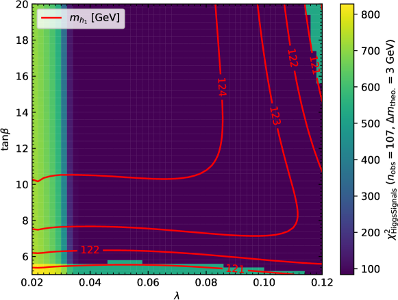
Figure 2: Result of the $\chi^{2}$-test regarding the signal rates of the SM Higgs boson using HiggsSignals. The colour coding indicates the value of $\chi^{2}$. The reference value of the SM regarding the same set of observables is $\chi^{2}_{\rm SM}=84$. The red lines are contour lines indicating the value of the SM-like Higgs-boson mass $m_{h_{1}}$.

In Fig. 2 we summary the results related to the SM-like Higgs boson $h_{1}$. We indicate the mass $m_{h_{1}}$ with the red contours. Assuming a theoretical uncertainty of $\sim 3\ \mathrm{GeV}$, one can see that a large fraction of the parameter space accommodates the Higgs-boson mass accurately. Only for values of $\tan\beta<6$ and $\lambda\sim 0.12$ we find points for which $m_{h_{1}}$ drops below $122\ \mathrm{GeV}$. The corrections to $m_{h_{1}}$ stemming from contributions beyond one-loop level are roughly of the size of $\sim 10\ \mathrm{GeV}$ in this scan. This demonstrates the importances of supplementing these corrections via the link to FeynHiggs. We can also see in Fig. 2 that the HiggsSignals test returns low values of $\chi^{2}<100$ for $n_{\rm obs}=107$ observables in the region where $m_{h_{1}}$ lies in the range $125\pm 3\ \mathrm{GeV}$. The reference value assuming the SM prediction is $\chi^{2}_{\rm SM}=84$, which roughly coincides with the values of $\chi^{2}$ obtained for the $\mu\nu$SSM in the parameter space coloured in blue. The large values of $\chi^{2}$ for $\lambda<0.03$ are caused by the decay $h_{1}\rightarrow\chi^{0}_{4}\chi^{0}_{4}$, which becomes kinematically allowed there, spoiling the SM-like behaviour of $h_{1}$.

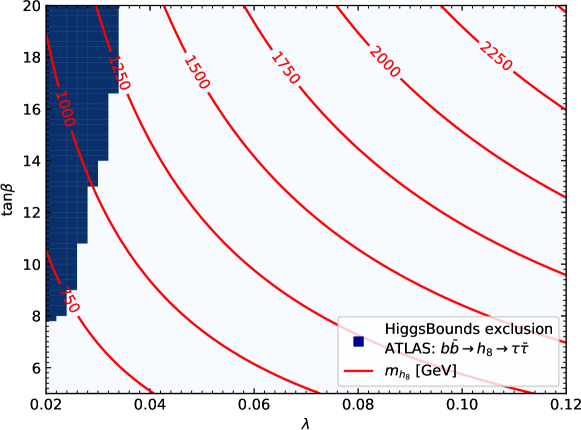
Figure 3: Result of the test against collider searches for additional Higgs bosons using HiggsBounds. The blue region is excluded at $95\%$ CL due to the search for additional Higgs bosons decaying into a pair of $\tau$ leptons of ATLAS [63]. The red lines are contour lines indicating the value of the heavy Higgs-boson mass $m_{h_{8}}$.

In Fig. 3 we depict the results of the HiggsBounds analysis. In this scenario, we find one experimental search that excludes a fraction of the parameter space for low $\lambda$ at the 95% confidence level. This is related to the fact that, as explained before, small values of $\lambda$ yield a small effective $\mu$-parameter. This reduces also the mass of the MSSM-like heavy Higgs boson $h_{8}$ (usually denoted $H$ in the MSSM). The mass $m_{h_{8}}$ is indicated by the red contours in Fig. 3. The relevant experimental search is the one for heavy Higgs bosons decaying into a pair of $\tau$ leptons using the LHC Run II data, corresponding to an integrated luminosity of $139\ \text{fb}^{-1}$, performed by ATLAS [63]. Both the $b\bar{b}$ associated production cross section as well as the decay width of $h_{8}$ into a pair of $\tau$ leptons roughly scale with $\tan^{2}\beta$. Thus, larger values of $\tan\beta$ exclude parameter points even when $m_{h_{8}}$ is considerably larger than $\sim 1\ \mathrm{TeV}$. For larger values of $\lambda$, the most sensitive experimental searches, as selected by HiggsBounds, are measurements regarding the cross section limits of the Higgs boson $h_{1}$ at $\sim 125\ \mathrm{GeV}$. This indicates that the predicted signal rates of the other Higgs bosons of the $\mu\nu$SSM are substantially below the experimental limits in most parts of the white region of Fig. 3.

5 Conclusion and outlook

In this paper we present the public code munuSSM: A flexible python package for the phenomenological analysis of the $\mu$-from-$\nu$ Supersymmetric Standard Model. The code incorporates a calculation of the radiatively corrected Higgs-boson masses. The precision of the prediction for the SM-like Higgs-boson mass is at a comparable level to the ones of spectrum generators for the MSSM. This is achieved by a full one-loop renormalization of the Higgs potential and consistently supplementing higher-order corrections known from the MSSM via an interface to the public code FeynHiggs. For obvious reasons, this approach does not capture effects beyond one-loop level genuine to the $\mu\nu$SSM. For the SM-like Higgs-boson mass, these contributions are expected to be substantially smaller than the MSSM-like contributions considered here for phenomenologically viable points. Nevertheless, for an estimate of the theory uncertainty this fact should be kept in mind.

In addition, the package munuSSM provides a calculation of effective couplings and branching ratios of the abundant scalars, pseudoscalars and sleptons of the model. Based on these quantities, a set of benchmark points can easily be checked against collider constraints from the Tevatron, LEP and the LHC via a user-friendly interface to the public code HiggsBounds. Furthermore, the presence in the spectrum of a Higgs boson reproducing the measured signal rates of the SM Higgs boson at $\sim 125\ \mathrm{GeV}$ can be verified via an interface to the public code HiggsSignals. Since both codes are accessed via their Fortran libraries, they can be utilized to extract other useful quantities which would not be directly accessible via the simpler command-line or SLHA-file input methods. For instance, we obtain the LHC cross sections for the neutral scalars as they are derived within HiggsBounds from the effective couplings. For a better interpretation of the HiggsSignals results, we provide a SM reference $\chi^{2}$ that can be taken into account when deciding whether a benchmark point is excluded or not.

The package munuSSM is a suitable framework for the implementation of further calculations and predictions related to the $\mu\nu$SSM. The modular structure of the code permits its extension without having to know the details of the already available features. In many cases, basic ingredients for the implementation of new features, such as the couplings and the mixing matrices, are already available, providing a starting point for the exploration of other sectors of the model (see also Tabs. LABEL:bpinitatt–LABEL:bpbrsatt for more details on the model definitions).

Appendix A Example input file

Listing 1: Example input file with random parameter values

⬇

# munuSSM SUSY PARAMETERS ###############################

15.0 # TanBe

0.0005 # vL_1

0.0005 # vL_2

0.0005 # vL_3

1000.0 # vR_1

1000.0 # vR_2

1000.0 # vR_3

0.08 # lam_1

0.08 # lam_2

0.08 # lam_3

0.3 # kap_111

0.0 # kap_112

0.0 # kap_113

0.0 # kap_122

0.0 # kap_123

0.0 # kap_133

0.3 # kap_222

0.0 # kap_223

0.0 # kap_233

0.3 # kap_333

1.0e-07 # Yv_11

0.0 # Yv_12

0.0 # Yv_13

0.0 # Yv_21

1.0e-07 # Yv_22

0.0 # Yv_23

0.0 # Yv_31

0.0 # Yv_32

1.0e-07 # Yv_33

# munuSSM SOFT PARAMETERS ###############################

0.0 # ml2_12

0.0 # ml2_13

0.0 # ml2_23

0.0 # mlHd2_1

0.0 # mlHd2_2

0.0 # mlHd2_3

0.0 # mv2_12

0.0 # mv2_13

0.0 # mv2_23

2250000.0 # mq2_11

2250000.0 # mq2_22

2250000.0 # mq2_33

2250000.0 # mu2_11

2250000.0 # mu2_22

2250000.0 # mu2_33

2250000.0 # md2_11

2250000.0 # md2_22

2250000.0 # md2_33

2250000.0 # me2_11

0.0 # me2_12

0.0 # me2_13

2250000.0 # me2_22

0.0 # me2_23

2250000.0 # me2_33

1000.0 # Au_11

1000.0 # Au_22

2800.0 # Au_33

1000.0 # Ad_11

1000.0 # Ad_22

1000.0 # Ad_33

1000.0 # Ae_11

0.0 # Ae_12

0.0 # Ae_13

0.0 # Ae_21

1000.0 # Ae_22

0.0 # Ae_23

0.0 # Ae_31

0.0 # Ae_32

1000.0 # Ae_33

-1000.0 # Av_11

0.0 # Av_12

0.0 # Av_13

0.0 # Av_21

-1000.0 # Av_22

0.0 # Av_23

0.0 # Av_31

0.0 # Av_32

-1000.0 # Av_33

1000.0 # Alam_1

1000.0 # Alam_2

1000.0 # Alam_3

-100.0 # Akap_111

0.0 # Akap_112

0.0 # Akap_113

0.0 # Akap_122

0.0 # Akap_123

0.0 # Akap_133

-100.0 # Akap_222

0.0 # Akap_223

0.0 # Akap_233

-100.0 # Akap_333

300.0 # M1

500.0 # M2

1700.0 # M3

Appendix B Return values and class attributes

In the following tables we list the attributes that are set for an instance of the class BenchmarkPoint and the return values for each method defined in the class. In most cases the objects listed in the tables are of type NumberQP or ArrayQP, as defined in the module dataObjects (see Sect. 3). We remind the reader that the values can be obtained in terms of regular floats or NumPy float arrays by typing a.float if a is of type NumberQP or ArrayQP.

Table 4: Class attributes set for an instance of the class BenchmarkPointFromFile during initialization. The second column shows the shape of the objects of the type arrayQP. If no shape is shown the object is of type numberQP.

self.__init__(file)
Delta		Value of the UV divergent piece of loop integrals $\Delta=1/\varepsilon^{\mathrm{UV}}$
MT_POLE		Top quark pole mass $M_{t}$
MB_MB		Bottom quark mass at the scale $\overline{m}_{b}(m_{b})$
ScaleFac		Renormalization scale in powers of $M_{t}$: $\mu_{R}/M_{t}$
DRbarScale		Input scale of $\smash{\overline{\mathrm{DR}}}$ parameters $\mu_{0}$
MW		Mass of the $W$ boson $M_{W}$
MZ		Mass of the $Z$ boson $M_{Z}$
GF		Fermi constant $G_{F}$
AlfaS		Strong QCD coupling constant $\alpha_{S}(M_{Z})$
MC		Charme quark mass $m_{c}$
MS		Strange quark mass $m_{s}$
MU		Up quark mass $m_{u}$
MD		Down quark mass $m_{d}$
ML		Tauon mass $m_{\tau}$
MM		Muon mass $m_{\mu}$
ME		Electron mass $m_{e}$
MT		SM-$\smash{\overline{\mathrm{MS}}}$ top quark mass $\overline{m}_{t}^{\smash{\overline{\mathrm{MS}}},\rm SM}(M_{t})$
MB		MSSM-$\smash{\overline{\mathrm{DR}}}$ bottom quark mass $\overline{m}_{b}^{\smash{\overline{\mathrm{DR}}},\rm MSSM}(M_{S})$
TB		Ratio of doublet vevs $\tan\beta$
vL	(3, )	Left-handed sneutrino vevs $v_{iL}$
vR	(3, )	Right-handed sneutrino vevs $v_{iR}$
lam	(3, )	Superpotential couplings $\lambda_{i}$
kap	(3, 3, 3)	Superpotential couplings $\kappa_{ijk}$
Yv	(3, 3)	Neutrino Yukawa couplings $Y^{\nu}_{ij}$
mlHd2	(3, )	Soft mass parameters $(m_{H_{d}\widetilde{L}}^{2})_{i}$
mq2	(3, 3)	Soft mass parameters $(m_{\widetilde{Q}}^{2})_{ij}$
mu2	(3, 3)	Soft mass parameters $(m_{\widetilde{u}}^{2})_{ij}$
md2	(3, 3)	Soft mass parameters $(m_{\widetilde{d}}^{2})_{ij}$
me2	(3, 3)	Soft mass parameters $(m_{\widetilde{e}}^{2})_{ij}$
Au	(3, 3)	Soft trilinear parameters $A^{u}_{ij}$
Ad	(3, 3)	Soft trilinear parameters $A^{d}_{ij}$
Ae	(3, 3)	Soft trilinear parameters $A^{e}_{ij}$
Av	(3, 3)	Soft trilinear parameters $A^{\nu}_{ij}$
Alam	(3, )	Soft trilinear parameters $A^{\lambda}_{i}$
Ak	(3, 3, 3)	Soft trilinear parameters $A^{\kappa}_{ijk}$
M1		Gaugino mass parameter $M_{1}$
M2		Gaugino mass parameter $M_{2}$
M3		Gaugino mass parameter $M_{3}$
CTW		Cosine of weak mixing angle $c_{w}$
STW		Sine of weak mixing angle $s_{w}$
g1		$\mathrm{U}(1)_{Y}$ gauge coupling $g_{1}$
g2		$\mathrm{SU}(2)_{L}$ gauge coupling $g_{2}$
g3		$\mathrm{SU}(3)_{c}$ gauge coupling $g_{3}$
v		SM vev $v$
vd		Down-type vev $v_{d}$
vu		Up-type vev $v_{u}$
Yu	(3, 3)	Up-type quark Yukawa couplings $Y^{u}_{ij}$
Yd	(3, 3)	Down-type quark Yukawa couplings $Y^{d}_{ij}$
Ye	(3, 3)	Charged lepton Yukawa couplings $Y^{e}_{ij}$
Tlam	(3, )	Soft trilinear couplings $T^{\lambda}_{i}$
Tk	(3, 3, 3)	Soft trilinear couplings $T^{\kappa}_{ijk}$
Tu	(3, 3)	Soft trilinear couplings $T^{u}_{ij}$
Td	(3, 3)	Soft trilinear couplings $T^{d}_{ij}$
Te	(3, 3)	Soft trilinear couplings $T^{e}_{ij}$
Tv	(3, 3)	Soft trilinear couplings $T^{\nu}_{ij}$
MuDimSq		Squared renormalization scale $\mu_{R}^{2}$
MUE		Effective $\mu$ parameter: $\mu=\lambda_{i}v_{iR}/\sqrt{2}$
mHd2		Down-type Higgs mass parameter $m_{H_{d}}^{2}$
mHu2		Up-type Higgs mass parameter $m_{H_{u}}^{2}$
mv2	(3, 3)	Right-handed sneutrino mass parameters $(m_{\widetilde{\nu}}^{2})_{ij}$
ml2	(3, 3)	Left-handed sneutrino and slepton mass parameters $(m_{\widetilde{L}}^{2})_{ij}$

Table 5: Class attributes set for an instance of the class BenchmarkPointFromFile by the method calc_tree_level_spectrum. The second column shows the shape of the objects of the type arrayQP.

self.calc_tree_level_spectrum()
MassSt	(2, )	Stop masses $m_{\widetilde{t}_{i}}$
ZT	(2, 2)	Stop mixing matrix $Z^{\widetilde{t}}_{ij}$
MassSc	(2, )	Scalar charme quark masses $m_{\widetilde{c}_{i}}$
ZC	(2, 2)	Scalar charme quark mixing matrix $Z^{\widetilde{c}}_{ij}$
MassSu	(2, )	Scalar up quark masses $m_{\widetilde{u}_{i}}$
ZU	(2, 2)	Scalar up quark mixing matrix $Z^{\widetilde{u}}_{ij}$
MassSb	(2, )	Sbottom masses $m_{\widetilde{b}_{i}}$
ZB	(2, 2)	Sbottom mixing matrix $Z^{\widetilde{b}}_{ij}$
MassSs	(2, )	Scalar strange quark masses $m_{\widetilde{s}_{i}}$
ZS	(2, 2)	Scalar strange quark mixing matrix $Z^{\widetilde{s}}_{ij}$
MassSd	(2, )	Scalar down quark masses $m_{\widetilde{d}_{i}}$
ZD	(2, 2)	Scalar down quark mixing matrix $Z^{\widetilde{d}}_{ij}$
Masshh	(8, )	Neutral CP-even scalar masses $m_{h_{i}}$
ZH	(8, 8)	Neutral CP-even scalar mixing matrix $Z^{h}_{ij}$
MassAh	(8, )	Neutral CP-odd scalar masses $m_{A_{i}}$ (including the Goldstone boson)
ZA	(8, 8)	Neutral CP-odd scalar mixing matrix $Z^{A}_{ij}$
MassHpm	(8, )	Charged scalar masses $m_{H^{\pm}_{i}}$ (including the Goldstone boson)
ZP	(8, 8)	Charged scalar mixing matrix $Z^{H^{\pm}}_{ij}$
MassCha	(5, )	Charged fermion masses $m_{\chi^{\pm}_{i}}$
ZEL	(5, 5)	Left-handed charged fermion mixing matrix $Z^{\chi^{\pm}_{L}}_{ij}$
ZER	(5, 5)	Right-handed charged fermion mixing matrix $Z^{\chi^{\pm}_{R}}_{ij}$
MassChi	(10, )	Neutral fermion masses $m_{\chi^{0}_{i}}$
UV_Re	(10, 10)	Real part of the neutral fermion mixing matrix $Z^{\chi^{0}}_{ij}$
UV_Im	(10, 10)	Imaginary part of the neutral fermion mixing matrix $Z^{\chi^{0}}_{ij}$

Table 6: Class attributes set for an instance of the class BenchmarkPointFromFile by the method calc_tree_level_couplings. The name of each attribute is given by cpl_[1]_[2] with [1] being the string given in the first column and [2] being Re for the real part and Im for the imaginary part of the couplings. The second column shows the shape of the objects of the type arrayQP. The couplings of fermions to scalars are decomposed as $\Gamma=\Gamma^{-}\omega^{-}+\Gamma^{+}\omega^{+}$ with $\omega^{\pm}=(1\pm\gamma_{5})/2$. The couplings of fermions to vector bosons are decomposed as $\Gamma_{\mu}=\Gamma^{-}\gamma_{\mu}\omega^{-}+\Gamma^{+}\gamma_{\mu}\omega^{+}$.

self.calc_tree_level_couplings()
hhhh	(8, 8, 8, 8)	$\Gamma_{h_{i}h_{j}h_{k}h_{l}}$	hhh	(8, 8, 8)	$\Gamma_{h_{i}h_{j}h_{k}}$
AAh	(8, 8, 8)	$\Gamma_{A_{i}A_{j}h_{k}}$	AAAA	(8, 8, 8, 8)	$\Gamma_{A_{i}A_{j}A_{k}A_{l}}$
AAhh	(8, 8, 8, 8)	$\Gamma_{A_{i}A_{j}h_{k}h_{l}}$	AXX	(8, 8, 8)	$\Gamma_{A_{i}H^{\pm}_{j}H^{\mp}_{k}}$
hXX	(8, 8, 8)	$\Gamma_{h_{i}H^{\pm}_{j}H^{\mp}_{k}}$	AAXX	(8, 8, 8, 8)	$\Gamma_{A_{i}A_{j}H^{\pm}_{k}H^{\mp}_{l}}$
AhXX	(8, 8, 8, 8)	$\Gamma_{A_{i}h_{j}H^{\pm}_{k}H^{\mp}_{l}}$	XXXX	(8, 8, 8, 8)	$\Gamma_{H^{\pm}_{i}H^{\mp}_{j}H^{\pm}_{k}H^{\mp}_{l}}$
hhXX	(8, 8, 8, 8)	$\Gamma_{h_{i}h_{j}H^{\pm}_{k}H^{\mp}_{l}}$
ChaChaA1	(5, 5, 8)	$\Gamma^{-}_{\chi^{\pm}_{i}\chi^{\mp}_{j}A_{k}}$	ChaChaA2	(5, 5, 8)	$\Gamma^{+}_{\chi^{\pm}_{i}\chi^{\mp}_{j}A_{k}}$
ChaChah1	(5, 5, 8)	$\Gamma^{-}_{\chi^{\pm}_{i}\chi^{\mp}_{j}h_{k}}$	ChaChah2	(5, 5, 8)	$\Gamma^{+}_{\chi^{\pm}_{i}\chi^{\mp}_{j}h_{k}}$
ChaChiX1	(5, 10, 8)	$\Gamma^{-}_{\chi^{\pm}_{i}\chi^{0}_{j}H^{\mp}_{k}}$	ChaChiX2	(5, 10, 8)	$\Gamma^{+}_{\chi^{\pm}_{i}\chi^{0}_{j}H^{\mp}_{k}}$
ChiChaX1	(10, 5, 8)	$\Gamma^{-}_{\chi^{0}_{i}\chi^{\mp}_{j}H^{\pm}_{k}}$	ChiChaX2	(10, 5, 8)	$\Gamma^{+}_{\chi^{0}_{i}\chi^{\mp}_{j}H^{\pm}_{k}}$
ChiChiA1	(10, 10, 8)	$\Gamma^{-}_{\chi^{0}_{i}\chi^{0}_{j}A_{k}}$	ChiChiA2	(10, 10, 8)	$\Gamma^{+}_{\chi^{0}_{i}\chi^{0}_{j}A_{k}}$
ChiChih1	(10, 10, 8)	$\Gamma^{-}_{\chi^{0}_{i}\chi^{0}_{j}h_{k}}$	ChiChih2	(10, 10, 8)	$\Gamma^{+}_{\chi^{0}_{i}\chi^{0}_{j}h_{k}}$
ChaChay1	(5, 5)	$\Gamma^{-}_{\chi^{\pm}_{i}\chi^{\mp}_{j}\gamma}$	ChaChay2	(5, 5)	$\Gamma^{+}_{\chi^{\pm}_{i}\chi^{\mp}_{j}\gamma}$
ChaChaZ1	(5, 5)	$\Gamma^{-}_{\chi^{\pm}_{i}\chi^{\mp}_{j}Z}$	ChaChaZ2	(5, 5)	$\Gamma^{+}_{\chi^{\pm}_{i}\chi^{\mp}_{j}Z}$
ChaChiW1	(5, 10)	$\Gamma^{-}_{\chi^{\pm}_{i}\chi^{0}_{j}W^{\mp}}$	ChaChiW2	(5, 10)	$\Gamma^{+}_{\chi^{\pm}_{i}\chi^{0}_{j}W^{\mp}}$
ChiChaW1	(10, 5)	$\Gamma^{-}_{\chi^{0}_{i}\chi^{\mp}_{j}W^{\pm}}$	ChiChaW2	(10, 5)	$\Gamma^{+}_{\chi^{0}_{i}\chi^{\pm}_{j}W^{\pm}}$
ChiChiZ1	(10, 10)	$\Gamma^{-}_{\chi^{0}_{i}\chi^{0}_{j}Z}$	ChiChiZ2	(10, 10)	$\Gamma^{+}_{\chi^{0}_{i}\chi^{0}_{j}Z}$
ASbSb	(8, 2, 2)	$2\Gamma_{A_{i}\widetilde{b}_{j}\widetilde{\overline{b}}_{k}}$	ASsSs	(8, 2, 2)	$2\Gamma_{A_{i}\widetilde{s}_{j}\widetilde{\overline{s}}_{k}}$
ASdSd	(8, 2, 2)	$2\Gamma_{A_{i}\widetilde{d}_{j}\widetilde{\overline{d}}_{k}}$	AStSt	(8, 2, 2)	$2\Gamma_{A_{i}\widetilde{t}_{j}\widetilde{\overline{t}}_{k}}$
AScSc	(8, 2, 2)	$2\Gamma_{A_{i}\widetilde{c}_{j}\widetilde{\overline{c}}_{k}}$	ASuSu	(8, 2, 2)	$2\Gamma_{A_{i}\widetilde{u}_{j}\widetilde{\overline{u}}_{k}}$
hSbSb	(8, 2, 2)	$12\Gamma_{h_{i}\widetilde{b}_{j}\widetilde{\overline{b}}_{k}}$	hSsSs	(8, 2, 2)	$12\Gamma_{h_{i}\widetilde{s}_{j}\widetilde{\overline{s}}_{k}}$
hSdSd	(8, 2, 2)	$12\Gamma_{h_{i}\widetilde{d}_{j}\widetilde{\overline{d}}_{k}}$	hStSt	(8, 2, 2)	$12\Gamma_{h_{i}\widetilde{t}_{j}\widetilde{\overline{t}}_{k}}$
hScSc	(8, 2, 2)	$12\Gamma_{h_{i}\widetilde{c}_{j}\widetilde{\overline{c}}_{k}}$	hSuSu	(8, 2, 2)	$12\Gamma_{h_{i}\widetilde{u}_{j}\widetilde{\overline{u}}_{k}}$
AASbSb	(8, 8, 2, 2)	$12\Gamma_{A_{i}A_{j}\widetilde{b}_{k}\widetilde{\overline{b}}_{l}}$	AASsSs	(8, 8, 2, 2)	$12\Gamma_{A_{i}A_{j}\widetilde{s}_{k}\widetilde{\overline{s}}_{l}}$
AASdSd	(8, 8, 2, 2)	$12\Gamma_{A_{i}A_{j}\widetilde{d}_{k}\widetilde{\overline{d}}_{l}}$	AAStSt	(8, 8, 2, 2)	$12\Gamma_{A_{i}A_{j}\widetilde{t}_{k}\widetilde{\overline{t}}_{l}}$
AAScSc	(8, 8, 2, 2)	$12\Gamma_{A_{i}A_{j}\widetilde{c}_{k}\widetilde{\overline{c}}_{l}}$	AASuSu	(8, 8, 2, 2)	$12\Gamma_{A_{i}A_{j}\widetilde{u}_{k}\widetilde{\overline{u}}_{l}}$
hhSbSb	(8, 8, 2, 2)	$12\Gamma_{h_{i}h_{j}\widetilde{b}_{k}\widetilde{\overline{b}}_{l}}$	hhSsSs	(8, 8, 2, 2)	$12\Gamma_{h_{i}h_{j}\widetilde{s}_{k}\widetilde{\overline{s}}_{l}}$
hhSdSd	(8, 8, 2, 2)	$12\Gamma_{h_{i}h_{j}\widetilde{d}_{k}\widetilde{\overline{d}}_{l}}$	hhStSt	(8, 8, 2, 2)	$12\Gamma_{h_{i}h_{j}\widetilde{t}_{k}\widetilde{\overline{t}}_{l}}$
hhScSc	(8, 8, 2, 2)	$12\Gamma_{h_{i}h_{j}\widetilde{c}_{k}\widetilde{\overline{c}}_{l}}$	hhSuSu	(8, 8, 2, 2)	$12\Gamma_{h_{i}h_{j}\widetilde{u}_{k}\widetilde{\overline{u}}_{l}}$
XXZ	(8, 8)	$\Gamma_{H^{\pm}_{i}H^{\mp}_{j}Z}$	XXy	(8, 8)	$\Gamma_{H^{\pm}_{i}H^{\mp}_{j}\gamma}$
XXZZ	(8, 8)	$\Gamma_{H^{\pm}_{i}H^{\mp}_{j}ZZ}$	XXyZ	(8, 8)	$\Gamma_{H^{\pm}_{i}H^{\mp}_{j}\gamma Z}$
XStSb	(8, 2, 2)	$4\Gamma_{H^{\pm}_{i}\widetilde{\overline{t}}_{j}\widetilde{b}_{k}}$	XScSs	(8, 2, 2)	$4\Gamma_{H^{\pm}_{i}\widetilde{\overline{c}}_{j}\widetilde{s}_{k}}$
XSuSd	(8, 2, 2)	$4\Gamma_{H^{\pm}_{i}\widetilde{\overline{u}}_{j}\widetilde{d}_{j}}$

Table 7: Class attributes set for an instance of the class BenchmarkPointFromFile by the method calc_one_loop_counterterms. The second column shows the shape of the objects of the type arrayQP. If no shape is shown the object is of the type numberQP. The counterterms are calculated including the UV divergent piece proportional to $\Delta=1/\varepsilon^{\rm UV}$ (see Tab. LABEL:bpinitatt) The exact definitions of the counterterms can be found in Ref. [4].

self.calc_one_loop_counterterms()
dZhh	(8, 8)	Field renormalization counterterms $\delta Z_{h_{i}h_{j}}$
dZAA	(8, 8)	Field renormalization counterterms $\delta Z_{A_{i}A_{j}}$
dTphi_Re	(8, )	Real part of the tadpole counterterms in the gauge basis $\mathrm{Re}(\delta T_{\phi_{i}})$
dTphi_Im	(8, )	Imaginary part of the tadpole counterterms in the gauge basis $\mathrm{Im}(\delta T_{\phi_{i}})$
dMW2		$W$-boson mass counterterm $\delta M_{W}^{2}$
dMZ2		$Z$-boson mass counterterm $\delta M_{Z}^{2}$
dmlHd2	(3, )	Soft mass parameter counterterms $(\delta m_{H_{d}\widetilde{L}}^{2})_{i}$
dml2Sum12		Soft mass parameter counterterm $\delta(m_{\widetilde{L}}^{2})_{12}$
dml2Sum13		Soft mass parameter counterterm $\delta(m_{\widetilde{L}}^{2})_{13}$
dml2Sum23		Soft mass parameter counterterm $\delta(m_{\widetilde{L}}^{2})_{23}$
dmv2Sum12		Soft mass parameter counterterm $\delta(m_{\widetilde{\nu}}^{2})_{12}$
dmv2Sum13		Soft mass parameter counterterm $\delta(m_{\widetilde{\nu}}^{2})_{13}$
dmv2Sum23		Soft mass parameter counterterm $\delta(m_{\widetilde{\nu}}^{2})_{23}$
dvL2	(3, )	Vev counterterms $\delta v_{iL}^{2}$
dvR2	(3, )	Vev counterterms $\delta v_{iR}^{2}$
dv2		Vev counterterm $\delta v^{2}$
dTanBe		Parameter counterterm $\delta\tan\beta$
dlam	(3, )	Superpotential parameter counterterms $\delta\lambda_{i}$
dkap	(3, 3, 3)	Superpotential parameter counterterms $\delta\kappa_{ijk}$
dYv	(3, 3)	Superpotential parameter counterterms $\delta Y^{\nu}_{ij}$
dTlam	(3, )	Soft parameter counterterms $\delta T^{\lambda}_{i}$
dTk	(3, 3, 3)	Soft parameter counterterms $\delta T^{\kappa}_{ijk}$
dM1		Gaugino mass parameter counterterm $\delta M_{1}$
dM2		Gaugino mass parameter counterterm $\delta M_{2}$
dM2phiphi_Re	(8, 8)	Real part of neutral CP-even scalar mass matrix counterterms in gauge basis $\mathrm{Re}(\delta M^{2}_{\phi_{i}\phi_{j}})$
dM2phiphi_Im	(8, 8)	Imaginary part of neutral CP-even scalar mass matrix counterterms in gauge basis $\mathrm{Im}(\delta M^{2}_{\phi_{i}\phi_{j}})$
dM2sigsig_Re	(8, 8)	Real part of neutral CP-odd scalar mass matrix counterterms in gauge basis $\mathrm{Re}(\delta M^{2}_{\sigma_{i}\sigma_{j}})$
dM2sigsig_Im	(8, 8)	Imaginary part of neutral CP-odd scalar mass matrix counterterms in gauge basis $\mathrm{Im}(\delta M^{2}_{\sigma_{i}\sigma_{j}})$
dM2hh_Re	(8, 8)	Real part of neutral CP-even scalar mass matrix counterterms in tree-level mass eigenstate basis $\mathrm{Re}(\delta M^{2}_{h_{i}h_{j}})$
dM2hh_Im	(8, 8)	Imaginary part of neutral CP-even scalar mass matrix counterterms in tree-level mass eigenstate basis $\mathrm{Im}(\delta M^{2}_{h_{i}h_{j}})$
dM2AA_Re	(8, 8)	Real part of neutral CP-odd scalar mass matrix counterterms in tree-level mass eigenstate basis $\mathrm{Re}(\delta M^{2}_{A_{i}A_{j}})$
dM2AA_Im	(8, 8)	Imaginary part of neutral CP-odd scalar mass matrix counterterms in tree-level mass eigenstate basis $\mathrm{Im}(\delta M^{2}_{A_{i}A_{j}})$

Table 8: The method calc_one_loop_self_energies of the class BenchmarkPointFromFile returns the values of the renormalized neutral scalar one-loop self energies at the given momentum. The returned object is a dictionary with the keys given in the first column. The first two keys are present if even=1 is chosen and the latter two keys are present if odd=1 is chosen. The values belonging to each key are objects of type arrayQP with the shape given in the second column.

self.calc_one_loop_self_energies(even,odd,p2_Re,p2_Im)
hhSERen_Re	(8, 8)	Real part of renormalized one-loop neutral CP-even self energies $\mathrm{Re}(\hat{\Sigma}_{h_{i}h_{j}}(p^{2}))$ with $\mathrm{Re}(p^{2})$ given as p2_Re and $\mathrm{Im}(p^{2})$ given as p2_Im
hhSERen_Im	(8, 8)	See above, but the imaginary part $\mathrm{Im}(\hat{\Sigma}_{h_{i}h_{j}}(p^{2}))$
AASERen_Re	(8, 8)	Real part of renormalized one-loop neutral CP-odd self energies $\mathrm{Re}(\hat{\Sigma}_{A_{i}A_{j}}(p^{2}))$ with $\mathrm{Re}(p^{2})$ given as p2_Re and $\mathrm{Im}(p^{2})$ given as p2_Im
AASERen_Im	(8, 8)	See above, but the imaginary part $\mathrm{Im}(\hat{\Sigma}_{h_{i}h_{j}}(p^{2}))$

Table 9: The method calc_two_loop_self_energies of the class BenchmarkPointFromFile returns the values of the renormalized neutral scalar self energies at the given momentum including higher-order corrections beyond one-loop level. The returned object is a dictionary with the keys given in the first column. The values belonging to each key are objects of type arrayQP with the shape given in the second column.

self.calc_two_loop_self_energies(p2_Re,p2_Im)
hhSERen_Re	(8, 8)	Real part of renormalized neutral CP-even self energies including corrections beyon one-loop level $\mathrm{Re}(\hat{\Sigma}_{h_{i}h_{j}}(p^{2}))$ with $\mathrm{Re}(p^{2})$ given as p2_Re and $\mathrm{Im}(p^{2})$ given as p2_Im
hhSERen_Im	(8, 8)	See above, but the imaginary part $\mathrm{Im}(\hat{\Sigma}_{h_{i}h_{j}}(p^{2}))$

Table 10: The method calc_loop_masses calculates the loop-corrected neutral scalar spectrum. For even=1 the attributes Masshh_L, ZH_L_Re and ZH_L_Im are set. For even=2 the attributes Masshh_2L_Re, ZH_2L_Re and ZH_2L_Im are set. For odd=1 the attributes MassAh_L, ZA_L_Re and ZA_L_Im are set. The values of each attribute are objects of type arrayQP with the shape given in the second column.

self.calc_loop_masses(even=2,odd=1,accu=1.e-5,momentum_mode=1)
Masshh_L	(8, )	Loop-corrected CP-even scalar masses at one-loop level $m_{h_{i}}^{(1)}$
ZH_L_Re	(8, 8)	Real part of loop-corrected CP-even scalar mixing matrix at one-loop level $\mathrm{Re}(Z^{h,(1)}_{ij})$
ZH_L_Im	(8, 8)	Imaginary part of loop-corrected CP-even scalar mixing matrix at one-loop level $\mathrm{Im}(Z^{h,(1)}_{ij})$
Masshh_2L	(8, )	Loop-corrected CP-even scalar masses including one-loop and higher-order corrections $m_{h_{i}}^{(2^{\prime})}$
ZH_2L_Re	(8, 8)	Real part of loop-corrected CP-even scalar mixing matrix including one-loop and higher-order corrections $\mathrm{Re}(Z^{h,(2^{\prime})}_{ij})$
ZH_L_Im	(8, 8)	Imaginary part of loop-corrected CP-even scalar mixing matrix including one-loop and higher-order corrections $\mathrm{Im}(Z^{h,(2^{\prime})}_{ij})$
MassAh_L	(8, )	Loop-corrected CP-odd scalar masses at one-loop level $m_{A_{i}}^{(1)}$ (including the goldstone boson)
ZA_L_Re	(8, 8)	Real part of loop-corrected CP-odd scalar mixing matrix at one-loop level $\mathrm{Re}(Z^{A,(1)}_{ij})$
ZA_L_Im	(8, 8)	Imaginary part of loop-corrected CP-odd scalar mixing matrix at one-loop level $\mathrm{Im}(Z^{A,(1)}_{ij})$

Table 11: The method calc_effective_couplings calculates the effective coupling coefficients, i.e., the couplings normalized to the SM prediction, for the neutral scalars. The couplings between $h_{i}A_{j}Z$, $h_{i}H^{\pm}_{j}W^{\mp}$ and $A_{i}H^{\pm}W^{\mp}$ do not have an analogue in the SM. Instead, $c_{h_{i}A_{j}Z}$ is given in factors of $e/(2s_{w}c_{w})$, and $c_{h_{i}H^{\pm}_{j}W^{\mp}}$ and $c_{A_{i}H^{\pm}_{j}W^{\mp}}$ in factors of $e/(2s_{w})$. The objects ScalarCpls and PseudoscalarCpls are set as attributes of the instance of BenchmarkPointFromFile. They are themselves instances of the classes Scalars and Pseudoscalars defined in the modules scalars and pseudoscalars of the subpackage effectiveCouplings. Thus, the first column shows the attributes of the instance of BenchmarkPointFromFile. They are NumPy arrays containing floats, with the shape given in the second column.

self.calc_effective_couplings()
ScalarCpls.chuu	(8, )	$c_{h_{i}u\bar{u}}$
ScalarCpls.chdd	(8, )	$c_{h_{i}d\bar{d}}$
ScalarCpls.chbb	(8, )	$c_{h_{i}b\bar{b}}$
ScalarCpls.chll	(8, )	$c_{h_{i}l\bar{l}}$
ScalarCpls.chtautau	(8, )	$c_{h_{i}\tau\bar{\tau}}$
ScalarCpls.chVV	(8, )	$c_{h_{i}VV}$
ScalarCpls.chgg	(8, )	$c_{h_{i}gg}$
ScalarCpls.chyy	(8, )	$c_{h_{i}\gamma\gamma}$
ScalarCpls.chAZ	(8, 8)	$c_{h_{i}A_{j}Z}$
Scalarcpls.chXW	(8, 8)	$c_{h_{i}H^{\pm}_{j}W^{\mp}}$
PseudoscalarCpls.cAuu	(8, )	$c_{A_{i}u\bar{u}}$
PseudoscalarCpls.cAdd	(8, )	$c_{A_{i}d\bar{d}}$
PseudoscalarCpls.cAbb	(8, )	$c_{A_{i}b\bar{b}}$
PseudoscalarCpls.cAll	(8, )	$c_{A_{i}l\bar{l}}$
PseudoscalarCpls.cAtautau	(8, )	$c_{A_{i}\tau\bar{\tau}}$
PseudoscalarCpls.cAVV	(8, )	$c_{A_{i}VV}$
PseudoscalarCpls.cAgg	(8, )	$c_{A_{i}gg}$
PseudoscalarCpls.cAyy	(8, )	$c_{A_{i}\gamma\gamma}$
Pseudocalarcpls.cAXW	(8, 8)	$c_{A_{i}H^{\pm}_{j}W^{\mp}}$

Table 12: The method calc_branching_ratios calculates the decay widths and the branching ratios of the neutral and charged scalars. The results are set as attributes Gammah, BranchingRatioh, GammaA, BranchingRatioA, GammaX and BranchingRatiosX, which are lists of dictionaries, to the instance of the class BenchmarkPointFromFile. Each dictionary contains the decay widths or branching ratios of a particle $h_{i}$, $A_{i}$ or $H^{\pm}_{i}$, where $i=1,8$ for the CP-even scalars and $i=1,7$ for the pseudoscalars and the charged scalars. The different final states of the decays as given in the fourth column correspond to the key values of the dictionaries given in the second column. The values corresponding to each key are floats if no shape is shown in the third column, and NumPy arrays with the given shape otherwise.

self.calc_branching_ratios()
Gammash[i]	hChiChi	(10, 10)	$\Gamma(h_{i}\rightarrow\chi^{0}_{j}\chi^{0}_{k})$
	hChaCha	(5, 5)	$\Gamma(h_{i}\rightarrow\chi^{\pm}_{j}\chi^{\mp}_{k})$
	hbb		$\Gamma(h_{i}\rightarrow b\bar{b})$
	htt		$\Gamma(h_{i}\rightarrow t\bar{t})$
	hcc		$\Gamma(h_{i}\rightarrow c\bar{c})$
	hss		$\Gamma(h_{i}\rightarrow s\bar{s})$
	hgg		$\Gamma(h_{i}\rightarrow gg)$
	hyy		$\Gamma(h_{i}\rightarrow\gamma\gamma)$
	hZZ		$\Gamma(h_{i}\rightarrow ZZ)$
	hWW		$\Gamma(h_{i}\rightarrow W^{\pm}W^{\mp})$
	hhh	(8, 8)	$\Gamma(h_{i}\rightarrow h_{j}h_{k})$
	hAA	(7, 7)	$\Gamma(h_{i}\rightarrow A_{j}A_{k})$
	hAZ	(7, )	$\Gamma(h_{i}\rightarrow A_{j}Z)$
	hXW	(7, 2)	$\Gamma(h_{i}\rightarrow H^{\pm,\mp}_{j}W^{\pm,\mp})$
	hXX	(7, 7)	$\Gamma(h_{i}\rightarrow H^{\pm}_{j}H^{\mp}_{k})$
	hStSt	(2, 2)	$\Gamma(h_{i}\rightarrow\widetilde{t}_{j}\widetilde{\bar{t}}_{k})$
	hScSc	(2, 2)	$\Gamma(h_{i}\rightarrow\widetilde{c}_{j}\widetilde{\bar{c}}_{k})$
	hSuSu	(2, 2)	$\Gamma(h_{i}\rightarrow\widetilde{u}_{j}\widetilde{\bar{u}}_{k})$
	hSbSb	(2, 2)	$\Gamma(h_{i}\rightarrow\widetilde{b}_{j}\widetilde{\bar{b}}_{k})$
	hSsSs	(2, 2)	$\Gamma(h_{i}\rightarrow\widetilde{s}_{j}\widetilde{\bar{s}}_{k})$
	hSdSd	(2, 2)	$\Gamma(h_{i}\rightarrow\widetilde{d}_{j}\widetilde{\bar{d}}_{k})$
	Tot		$\Gamma^{\rm Tot}_{h_{i}}$
BranchingRatiosh[i]	hChiChi	(10, 10)	$\mathrm{Br}(h_{i}\rightarrow\chi^{0}_{j}\chi^{0}_{k})$
	hChaCha	(5, 5)	$\mathrm{Br}(h_{i}\rightarrow\chi^{\pm}_{j}\chi^{\mp}_{k})$
	hbb		$\mathrm{Br}(h_{i}\rightarrow b\bar{b})$
	htt		$\mathrm{Br}(h_{i}\rightarrow t\bar{t})$
	hcc		$\mathrm{Br}(h_{i}\rightarrow c\bar{c})$
	hss		$\mathrm{Br}(h_{i}\rightarrow s\bar{s})$
	hgg		$\mathrm{Br}(h_{i}\rightarrow gg)$
	hyy		$\mathrm{Br}(h_{i}\rightarrow\gamma\gamma)$
	hZZ		$\mathrm{Br}(h_{i}\rightarrow ZZ)$
	hWW		$\mathrm{Br}(h_{i}\rightarrow W^{\pm}W^{\mp})$
	hhh	(8, 8)	$\mathrm{Br}(h_{i}\rightarrow h_{j}h_{k})$
	hAA	(7, 7)	$\mathrm{Br}(h_{i}\rightarrow A_{j}A_{k})$
	hAZ	(7, )	$\mathrm{Br}(h_{i}\rightarrow A_{j}Z)$
	hXW	(7, 2)	$\mathrm{Br}(h_{i}\rightarrow H^{\pm,\mp}_{j}W^{\pm,\mp})$
	hXX	(7, 7)	$\mathrm{Br}(h_{i}\rightarrow H^{\pm}_{j}H^{\mp}_{k})$
	hStSt	(2, 2)	$\mathrm{Br}(h_{i}\rightarrow\widetilde{t}_{j}\widetilde{\bar{t}}_{k})$
	hScSc	(2, 2)	$\mathrm{Br}(h_{i}\rightarrow\widetilde{c}_{j}\widetilde{\bar{c}}_{k})$
	hSuSu	(2, 2)	$\mathrm{Br}(h_{i}\rightarrow\widetilde{u}_{j}\widetilde{\bar{u}}_{k})$
	hSbSb	(2, 2)	$\mathrm{Br}(h_{i}\rightarrow\widetilde{b}_{j}\widetilde{\bar{b}}_{k})$
	hSsSs	(2, 2)	$\mathrm{Br}(h_{i}\rightarrow\widetilde{s}_{j}\widetilde{\bar{s}}_{k})$
	hSdSd	(2, 2)	$\mathrm{Br}(h_{i}\rightarrow\widetilde{d}_{j}\widetilde{\bar{d}}_{k})$
GammasA[i]	AChiChi	(10, 10)	$\Gamma(A_{i}\rightarrow\chi^{0}_{j}\chi^{0}_{k})$
	AChaCha	(5, 5)	$\Gamma(A_{i}\rightarrow\chi^{\pm}_{j}\chi^{\mp}_{k})$
	Abb		$\Gamma(A_{i}\rightarrow b\bar{b})$
	Att		$\Gamma(A_{i}\rightarrow t\bar{t})$
	Acc		$\Gamma(A_{i}\rightarrow c\bar{c})$
	Ass		$\Gamma(A_{i}\rightarrow s\bar{s})$
	Agg		$\Gamma(A_{i}\rightarrow gg)$
	Ayy		$\Gamma(A_{i}\rightarrow\gamma\gamma)$
	AAh	(7, 8)	$\Gamma(A_{i}\rightarrow A_{j}h_{k})$
	AhZ	(8, )	$\Gamma(A_{i}\rightarrow h_{h}Z)$
	AXW	(7, 2)	$\Gamma(A_{i}\rightarrow H^{\pm,\mp}_{j}W^{\pm,\mp})$
	AXX	(7, 7)	$\Gamma(A_{i}\rightarrow H^{\pm}_{j}H^{\mp}_{k})$
	AStSt	(2, 2)	$\Gamma(A_{i}\rightarrow\widetilde{t}_{j}\widetilde{\bar{t}}_{k})$
	AScSc	(2, 2)	$\Gamma(A_{i}\rightarrow\widetilde{c}_{j}\widetilde{\bar{c}}_{k})$
	ASuSu	(2, 2)	$\Gamma(A_{i}\rightarrow\widetilde{u}_{j}\widetilde{\bar{u}}_{k})$
	ASbSb	(2, 2)	$\Gamma(A_{i}\rightarrow\widetilde{b}_{j}\widetilde{\bar{b}}_{k})$
	ASsSs	(2, 2)	$\Gamma(A_{i}\rightarrow\widetilde{s}_{j}\widetilde{\bar{s}}_{k})$
	ASdSd	(2, 2)	$\Gamma(A_{i}\rightarrow\widetilde{d}_{j}\widetilde{\bar{d}}_{k})$
	Tot		$\Gamma^{\rm Tot}_{A_{i}}$
BranchingRatiosA[i]	AChiChi	(10, 10)	$\mathrm{Br}(A_{i}\rightarrow\chi^{0}_{j}\chi^{0}_{k})$
	AChaCha	(5, 5)	$\mathrm{Br}(A_{i}\rightarrow\chi^{\pm}_{j}\chi^{\mp}_{k})$
	Abb		$\mathrm{Br}(A_{i}\rightarrow b\bar{b})$
	Att		$\mathrm{Br}(A_{i}\rightarrow t\bar{t})$
	Acc		$\mathrm{Br}(A_{i}\rightarrow c\bar{c})$
	Ass		$\mathrm{Br}(A_{i}\rightarrow s\bar{s})$
	Agg		$\mathrm{Br}(A_{i}\rightarrow gg)$
	Ayy		$\mathrm{Br}(A_{i}\rightarrow\gamma\gamma)$
	AAh	(7, 8)	$\mathrm{Br}(A_{i}\rightarrow A_{j}h_{k})$
	AhZ	(8, )	$\mathrm{Br}(A_{i}\rightarrow h_{h}Z)$
	AXW	(7, 2)	$\mathrm{Br}(A_{i}\rightarrow H^{\pm,\mp}_{j}W^{\pm,\mp})$
	AXX	(7, 7)	$\mathrm{Br}(A_{i}\rightarrow H^{\pm}_{j}H^{\mp}_{k})$
	AStSt	(2, 2)	$\mathrm{Br}(A_{i}\rightarrow\widetilde{t}_{j}\widetilde{\bar{t}}_{k})$
	AScSc	(2, 2)	$\mathrm{Br}(A_{i}\rightarrow\widetilde{c}_{j}\widetilde{\bar{c}}_{k})$
	ASuSu	(2, 2)	$\mathrm{Br}(A_{i}\rightarrow\widetilde{u}_{j}\widetilde{\bar{u}}_{k})$
	ASbSb	(2, 2)	$\mathrm{Br}(A_{i}\rightarrow\widetilde{b}_{j}\widetilde{\bar{b}}_{k})$
	ASsSs	(2, 2)	$\mathrm{Br}(A_{i}\rightarrow\widetilde{s}_{j}\widetilde{\bar{s}}_{k})$
	ASdSd	(2, 2)	$\mathrm{Br}(A_{i}\rightarrow\widetilde{d}_{j}\widetilde{\bar{d}}_{k})$
GammasX[i]	XhX	(8, 7)	$\Gamma(H^{\pm}_{i}\rightarrow h_{j}H^{\pm}_{k})$
	XAX	(7, 7)	$\Gamma(H^{\pm}_{i}\rightarrow A_{j}H^{\pm}_{k})$
	XStSb	(2, 2)	$\Gamma(H^{\pm}_{i}\rightarrow\widetilde{t}_{j}\widetilde{\bar{b}}_{k})$
	XScSs	(2, 2)	$\Gamma(H^{\pm}_{i}\rightarrow\widetilde{c}_{j}\widetilde{\bar{s}}_{k})$
	XSuSd	(2, 2)	$\Gamma(H^{\pm}_{i}\rightarrow\widetilde{u}_{j}\widetilde{\bar{d}}_{k})$
	XhW	(8, )	$\Gamma(H^{\pm}_{i}\rightarrow h_{j}W^{\pm})$
	XAW	(7, )	$\Gamma(H^{\pm}_{i}\rightarrow A_{j}W^{\pm})$
	XChaChi	(5, 10)	$\Gamma(H^{\pm}_{i}\rightarrow\chi^{\pm}_{j}\chi^{0}_{k})$
	Xtb		$\Gamma(H^{\pm}_{i}\rightarrow t\bar{b})$
	Xcs		$\Gamma(H^{\pm}_{i}\rightarrow c\bar{s})$
	Tot		$\Gamma^{\rm Tot}_{H^{\pm}_{i}}$

References

- Lopez-Fogliani and Muñoz [2006] D. Lopez-Fogliani and C. Muñoz, “Proposal for a Supersymmetric Standard Model”, Phys. Rev. Lett. 97 (2006) 041801, hep-ph/0508297.
- Muñoz [2010] C. Muñoz, “Phenomenology of a New Supersymmetric Standard Model: The mu nu SSM”, AIP Conf. Proc. 1200 (2010), no. 1, 413–416, arXiv:0909.5140.
- Biekötter et al. [2018] T. Biekötter, S. Heinemeyer, and C. Muñoz, “Precise prediction for the Higgs-boson masses in the SSM”, Eur. Phys. J. C 78 (2018), no. 6, 504, arXiv:1712.07475.
- Biekötter et al. [2019] T. Biekötter, S. Heinemeyer, and C. Muñoz, “Precise prediction for the Higgs-Boson masses in the SSM with three right-handed neutrino superfields”, Eur. Phys. J. C 79 (2019), no. 8, 667, arXiv:1906.06173.
- Zhang [1999] R.-J. Zhang, “Two loop effective potential calculation of the lightest CP even Higgs boson mass in the MSSM”, Phys. Lett. B 447 (1999) 89–97, hep-ph/9808299.
- Espinosa and Zhang [2000] J. R. Espinosa and R.-J. Zhang, “MSSM lightest CP even Higgs boson mass to O(alpha(s) alpha(t)): The Effective potential approach”, JHEP 03 (2000) 026, hep-ph/9912236.
- Heinemeyer et al. [1999] S. Heinemeyer, W. Hollik, and G. Weiglein, “The Masses of the neutral CP - even Higgs bosons in the MSSM: Accurate analysis at the two loop level”, Eur. Phys. J. C 9 (1999) 343–366, hep-ph/9812472.
- Kpatcha et al. [2020] E. Kpatcha, R. Ruiz de Austri, D. E. López-Fogliani, and C. Muñoz, “Impact of Higgs physics on the parameter space of the ”, Eur. Phys. J. C 80 (2020), no. 4, 336, arXiv:1910.08062.
- Ghosh et al. [2018] P. Ghosh, I. Lara, D. E. Lopez-Fogliani, C. Muñoz, and R. Ruiz de Austri, “Searching for left sneutrino LSP at the LHC”, Int. J. Mod. Phys. A 33 (2018), no. 18n19, 1850110, arXiv:1707.02471.
- Lara et al. [2018] I. Lara, D. E. López-Fogliani, C. Muñoz, N. Nagata, H. Otono, and R. Ruiz De Austri, “Looking for the left sneutrino LSP with displaced-vertex searches”, Phys. Rev. D 98 (2018), no. 7, 075004, arXiv:1804.00067.
- Kpatcha et al. [2019] E. Kpatcha, I. Lara, D. E. López-Fogliani, C. Muñoz, N. Nagata, H. Otono, and R. Ruiz De Austri, “Sampling the SSM for displaced decays of the tau left sneutrino LSP at the LHC”, Eur. Phys. J. C 79 (2019), no. 11, 934, arXiv:1907.02092.
- Porod [2003] W. Porod, “SPheno, a program for calculating supersymmetric spectra, SUSY particle decays and SUSY particle production at e+ e- colliders”, Comput. Phys. Commun. 153 (2003) 275–315, hep-ph/0301101.
- Porod and Staub [2012] W. Porod and F. Staub, “SPheno 3.1: Extensions including flavour, CP-phases and models beyond the MSSM”, Comput. Phys. Commun. 183 (2012) 2458–2469, arXiv:1104.1573.
- Staub [2010] F. Staub, “From Superpotential to Model Files for FeynArts and CalcHep/CompHep”, Comput. Phys. Commun. 181 (2010) 1077–1086, arXiv:0909.2863.
- Staub [2011] F. Staub, “Automatic Calculation of supersymmetric Renormalization Group Equations and Self Energies”, Comput. Phys. Commun. 182 (2011) 808–833, arXiv:1002.0840.
- Staub [2013] F. Staub, “SARAH 3.2: Dirac Gauginos, UFO output, and more”, Comput. Phys. Commun. 184 (2013) 1792–1809, arXiv:1207.0906.
- Staub [2014] F. Staub, “SARAH 4 : A tool for (not only SUSY) model builders”, Comput. Phys. Commun. 185 (2014) 1773–1790, arXiv:1309.7223.
- Athron et al. [2015] P. Athron, J.-h. Park, D. Stöckinger, and A. Voigt, “FlexibleSUSY—A spectrum generator generator for supersymmetric models”, Comput. Phys. Commun. 190 (2015) 139–172, arXiv:1406.2319.
- Athron et al. [2017] P. Athron, J.-h. Park, T. Steudtner, D. Stöckinger, and A. Voigt, “Precise Higgs mass calculations in (non-)minimal supersymmetry at both high and low scales”, JHEP 01 (2017) 079, arXiv:1609.00371.
- Athron et al. [2018] P. Athron, M. Bach, D. Harries, T. Kwasnitza, J.-h. Park, D. Stöckinger, A. Voigt, and J. Ziebell, “FlexibleSUSY 2.0: Extensions to investigate the phenomenology of SUSY and non-SUSY models”, Comput. Phys. Commun. 230 (2018) 145–217, arXiv:1710.03760.
- Heinemeyer et al. [2000] S. Heinemeyer, W. Hollik, and G. Weiglein, “FeynHiggs: A Program for the calculation of the masses of the neutral CP even Higgs bosons in the MSSM”, Comput. Phys. Commun. 124 (2000) 76–89, hep-ph/9812320.
- Degrassi et al. [2003] G. Degrassi, S. Heinemeyer, W. Hollik, P. Slavich, and G. Weiglein, “Towards high precision predictions for the MSSM Higgs sector”, Eur. Phys. J. C 28 (2003) 133–143, hep-ph/0212020.
- Frank et al. [2007] M. Frank, T. Hahn, S. Heinemeyer, W. Hollik, H. Rzehak, and G. Weiglein, “The Higgs Boson Masses and Mixings of the Complex MSSM in the Feynman-Diagrammatic Approach”, JHEP 02 (2007) 047, hep-ph/0611326.
- Hahn et al. [2014] T. Hahn, S. Heinemeyer, W. Hollik, H. Rzehak, and G. Weiglein, “High-Precision Predictions for the Light CP -Even Higgs Boson Mass of the Minimal Supersymmetric Standard Model”, Phys. Rev. Lett. 112 (2014), no. 14, 141801, arXiv:1312.4937.
- Bahl and Hollik [2016] H. Bahl and W. Hollik, “Precise prediction for the light MSSM Higgs boson mass combining effective field theory and fixed-order calculations”, Eur. Phys. J. C 76 (2016), no. 9, 499, arXiv:1608.01880.
- Bahl et al. [2018] H. Bahl, S. Heinemeyer, W. Hollik, and G. Weiglein, “Reconciling EFT and hybrid calculations of the light MSSM Higgs-boson mass”, Eur. Phys. J. C 78 (2018), no. 1, 57, arXiv:1706.00346.
- Bahl et al. [2020] H. Bahl, T. Hahn, S. Heinemeyer, W. Hollik, S. Paßehr, H. Rzehak, and G. Weiglein, “Precision calculations in the MSSM Higgs-boson sector with FeynHiggs 2.14”, Comput. Phys. Commun. 249 (2020) 107099, arXiv:1811.09073.
- Heinemeyer et al. [2013] LHC Higgs Cross Section Working Group Collaboration, S. Heinemeyer, C. Mariotti, G. Passarino, R. Tanaka, et al., “Handbook of LHC Higgs Cross Sections: 3. Higgs Properties”, arXiv:1307.1347.
- de Florian et al. [2016] LHC Higgs Cross Section Working Group Collaboration, D. de Florian et al., “Handbook of LHC Higgs Cross Sections: 4. Deciphering the Nature of the Higgs Sector”, arXiv:1610.07922.
- Bechtle et al. [2010] P. Bechtle, O. Brein, S. Heinemeyer, G. Weiglein, and K. E. Williams, “HiggsBounds: Confronting Arbitrary Higgs Sectors with Exclusion Bounds from LEP and the Tevatron”, Comput. Phys. Commun. 181 (2010) 138–167, arXiv:0811.4169.
- Bechtle et al. [2011] P. Bechtle, O. Brein, S. Heinemeyer, G. Weiglein, and K. E. Williams, “HiggsBounds 2.0.0: Confronting Neutral and Charged Higgs Sector Predictions with Exclusion Bounds from LEP and the Tevatron”, Comput. Phys. Commun. 182 (2011) 2605–2631, arXiv:1102.1898.
- Bechtle et al. [2012] P. Bechtle, O. Brein, S. Heinemeyer, O. Stal, T. Stefaniak, G. Weiglein, and K. Williams, “Recent Developments in HiggsBounds and a Preview of HiggsSignals”, PoS CHARGED2012 (2012) 024, arXiv:1301.2345.
- Bechtle et al. [2014] P. Bechtle, O. Brein, S. Heinemeyer, O. Stål, T. Stefaniak, G. Weiglein, and K. E. Williams, “: Improved Tests of Extended Higgs Sectors against Exclusion Bounds from LEP, the Tevatron and the LHC”, Eur. Phys. J. C 74 (2014), no. 3, 2693, arXiv:1311.0055.
- Bechtle et al. [2015] P. Bechtle, S. Heinemeyer, O. Stal, T. Stefaniak, and G. Weiglein, “Applying Exclusion Likelihoods from LHC Searches to Extended Higgs Sectors”, Eur. Phys. J. C 75 (2015), no. 9, 421, arXiv:1507.06706.
- Bechtle et al. [2020] P. Bechtle, D. Dercks, S. Heinemeyer, T. Klingl, T. Stefaniak, G. Weiglein, and J. Wittbrodt, “HiggsBounds-5: Testing Higgs Sectors in the LHC 13 TeV Era”, arXiv:2006.06007.
- Bechtle et al. [2014] P. Bechtle, S. Heinemeyer, O. Stål, T. Stefaniak, and G. Weiglein, “: Confronting arbitrary Higgs sectors with measurements at the Tevatron and the LHC”, Eur. Phys. J. C 74 (2014), no. 2, 2711, arXiv:1305.1933.
- Stål and Stefaniak [2013] O. Stål and T. Stefaniak, “Constraining extended Higgs sectors with HiggsSignals”, PoS EPS-HEP2013 (2013) 314, arXiv:1310.4039.
- Bechtle et al. [2014] P. Bechtle, S. Heinemeyer, O. Stål, T. Stefaniak, and G. Weiglein, “Probing the Standard Model with Higgs signal rates from the Tevatron, the LHC and a future ILC”, JHEP 11 (2014) 039, arXiv:1403.1582.
- Bechtle et al. [2020] P. Bechtle, S. Heinemeyer, T. Klingl, T. Stefaniak, G. Weiglein, and J. Wittbrodt, “HiggsSignals-2: Probing new physics with precision Higgs measurements in the LHC 13 TeV era”, arXiv:2012.09197.
- Lopez-Fogliani and Muñoz [2020] D. E. Lopez-Fogliani and C. Muñoz, “Searching for Supersymmetry: The SSM”, arXiv:2009.01380.
- Brignole et al. [1998] A. Brignole, L. E. Ibanez, and C. Muñoz, “Soft supersymmetry breaking terms from supergravity and superstring models”, Adv. Ser. Direct. High Energy Phys. 18 (1998) 125–148, arXiv:hep-ph/9707209.
- Biekötter [2019] T. Biekötter, “Phenomenology of the Higgs sectors of the SSM and the N2HDM”, PhD thesis, U. Autonoma, Madrid (main), 2019.
- Hahn [2001] T. Hahn, “Generating Feynman diagrams and amplitudes with FeynArts 3”, Comput. Phys. Commun. 140 (2001) 418–431, arXiv:hep-ph/0012260.
- Gómez-Vargas et al. [2020] G. A. Gómez-Vargas, D. E. López-Fogliani, C. Muñoz, and A. D. Perez, “MeV-GeV -ray telescopes probing axino LSP/gravitino NLSP as dark matter in the SSM”, JCAP 01 (2020) 058, arXiv:1911.03191.
- Gómez-Vargas et al. [2019] G. A. Gómez-Vargas, D. E. López-Fogliani, C. Muñoz, and A. D. Perez, “MeV-GeV -ray telescopes probing gravitino LSP with coexisting axino NLSP as dark matter in the SSM”, arXiv:1911.08550.
- Hahn and Perez-Victoria [1999] T. Hahn and M. Perez-Victoria, “Automatized one loop calculations in four-dimensions and D-dimensions”, Comput. Phys. Commun. 118 (1999) 153–165, hep-ph/9807565.
- Draper and Rzehak [2016] P. Draper and H. Rzehak, “A Review of Higgs Mass Calculations in Supersymmetric Models”, Phys. Rept. 619 (2016) 1–24, arXiv:1601.01890.
- Ellwanger et al. [2010] U. Ellwanger, C. Hugonie, and A. M. Teixeira, “The Next-to-Minimal Supersymmetric Standard Model”, Phys. Rept. 496 (2010) 1–77, arXiv:0910.1785.
- Harris et al. [2020] C. R. Harris et al., “Array programming with NumPy”, Nature 585 (2020), no. 7825, 357–362, arXiv:2006.10256.
- Djouadi et al. [1998] A. Djouadi, J. Kalinowski, and M. Spira, “HDECAY: A Program for Higgs boson decays in the standard model and its supersymmetric extension”, Comput. Phys. Commun. 108 (1998) 56–74, hep-ph/9704448.
- Spira [1998] M. Spira, “QCD effects in Higgs physics”, Fortsch. Phys. 46 (1998) 203–284, hep-ph/9705337.
- Butterworth et al. [2010] J. Butterworth et al., “THE TOOLS AND MONTE CARLO WORKING GROUP Summary Report from the Les Houches 2009 Workshop on TeV Colliders”, in “6th Les Houches Workshop on Physics at TeV Colliders”. 3 2010. arXiv:1003.1643.
- Bredenstein et al. [2006] A. Bredenstein, A. Denner, S. Dittmaier, and M. Weber, “Precise predictions for the Higgs-boson decay H WW/ZZ 4 leptons”, Phys. Rev. D 74 (2006) 013004, hep-ph/0604011.
- Bredenstein et al. [2007] A. Bredenstein, A. Denner, S. Dittmaier, and M. Weber, “Radiative corrections to the semileptonic and hadronic Higgs-boson decays H W W / Z Z 4 fermions”, JHEP 02 (2007) 080, hep-ph/0611234.
- Goodsell et al. [2017] M. D. Goodsell, S. Liebler, and F. Staub, “Generic calculation of two-body partial decay widths at the full one-loop level”, Eur. Phys. J. C 77 (2017), no. 11, 758, arXiv:1703.09237.
- Spira [2017] M. Spira, “Higgs Boson Production and Decay at Hadron Colliders”, Prog. Part. Nucl. Phys. 95 (2017) 98–159, arXiv:1612.07651.
- Drechsel et al. [2017] P. Drechsel, R. Gröber, S. Heinemeyer, M. M. Muhlleitner, H. Rzehak, and G. Weiglein, “Higgs-Boson Masses and Mixing Matrices in the NMSSM: Analysis of On-Shell Calculations”, Eur. Phys. J. C 77 (2017), no. 6, 366, arXiv:1612.07681.
- Hollik et al. [2019a] W. G. Hollik, S. Liebler, G. Moortgat-Pick, S. Paßehr, and G. Weiglein, “Phenomenology of the inflation-inspired NMSSM at the electroweak scale”, Eur. Phys. J. C 79 (2019)a, no. 1, 75, arXiv:1809.07371.
- Hollik et al. [2019b] W. G. Hollik, S. Liebler, G. Moortgat-Pick, S. Paßehr, and G. Weiglein, “Phenomenological consequences of Higgs inflation in the NMSSM at the electroweak scale”, PoS ICHEP2018 (2019)b 455, arXiv:1811.12838.
- Hahn [2006] T. Hahn, “Routines for the diagonalization of complex matrices”, physics/0607103.
- Wes McKinney [2010] Wes McKinney, “Data Structures for Statistical Computing in Python”, in “Proceedings of the 9th Python in Science Conference”, Stéfan van der Walt and Jarrod Millman, eds., pp. 56 – 61. 2010.
- Hunter [2007] J. D. Hunter, “Matplotlib: A 2d graphics environment”, Computing in Science & Engineering 9 (2007), no. 3, 90–95.
- Aad et al. [2020] ATLAS Collaboration, G. Aad et al., “Search for heavy Higgs bosons decaying into two tau leptons with the ATLAS detector using collisions at TeV”, Phys. Rev. Lett. 125 (2020), no. 5, 051801, arXiv:2002.12223.