Predicting Sim-to-Real Transfer of RL Policies
with Probabilistic Dynamics Models

Abstract

We propose a method to predict the sim-to-real transfer performance of RL policies. Our transfer metric simplifies the selection of training setups (such as algorithm, hyperparameters, randomizations) and policies in simulation, without the need for extensive and time-consuming real-world rollouts. A probabilistic dynamics model is trained alongside the policy and evaluated on a fixed set of real-world trajectories to obtain the transfer metric. Experiments show that the transfer metric is highly correlated with policy performance in both simulated and real-world robotic environments for complex manipulation tasks. We further show that the transfer metric can predict the effect of training setups on policy transfer performance.

1 Introduction

Many recent advances in deep reinforcement learning (RL) for robotics have been achieved by training in simulation and zero (or few) shot transfer to a real environment (Tan et al., 2018; Peng et al., 2018; Golemo et al., 2018; OpenAI et al., 2018; Hwangbo et al., 2019; OpenAI et al., 2019). The key advantage of this approach is the availability of efficient and scalable environment interactions in simulation and is well-suited to powerful deep RL algorithms (Schulman et al., 2017; Haarnoja et al., 2018b). However, policies trained in simulation often do not achieve the same level of performance in the real environment. This is known as the sim-to-real transfer problem.

Domain randomization (DR) (Tobin et al., 2017; Sadeghi & Levine, 2017; Peng et al., 2018) is a promising technique which helps to resolve the sim-to-real transfer problem. In DR, a policy is trained using data generated from a diverse set of environments. The environments are sampled from a distribution defined by a set of manually tuned parameters (Tobin et al., 2017; Sadeghi & Levine, 2017; Peng et al., 2018; OpenAI et al., 2018). Success of DR depends on the parameter tuning, which involves iterating between policy training and real-world deployment. This iterative process is slow, prone to failures, and human dependent.

Automatic domain randomization (ADR) (OpenAI et al., 2019) improves on DR by automatically adjusting the environment distribution based on policy performance. However, ADR suffers from a similar iterative process as DR, since it is difficult to know when the environment distribution is sufficient to produce good transfer.

In this work, we introduce a method to predict the transfer performance of policies trained in simulation, using only a fixed set of real-world trajectories. We show that the proposed transfer metric strongly correlates with policy transfer performance. For DR training, we show that the transfer metric can predict the transfer performance of policies trained using different environment distribution parameters. For ADR training, we show that the transfer metric can predict relative changes in transfer performance as training progresses and can be used as an effective indicator for stopping ADR.

2 Related Works

A number of methods that use real-world data to improve sim-to-real performance have been proposed. Neural networks were trained to predict and compensate for discrepancies between simulated and real-world trajectories (Golemo et al., 2018; Hwangbo et al., 2019). An inverse dynamics model was trained using real-world rollouts and used to adjust policy outputs during deployment (Christiano et al., 2016). A policy network was trained in simulation then progressively modified in the real-world environment to improve performance (Rusu et al., 2016). These methods rely on a large amount of real-world trajectories to train neural networks, limiting their scope of application.

Works on predicting transfer performance have been suggested for evolution strategies (Koos et al., 2010) with evaluation on a fixed set of real-world trajectories (Farchy et al., 2013; Hanna & Stone, 2017). The grounded simulation learning (GSL) technique proposed in (Hanna & Stone, 2017) optimizes the simulator based on its predictions on real-world trajectories. Our work implements a similar idea by using a more flexible (and differentiable) dynamics model.

For deep RL policies trained under DR, (Muratore et al., 2018) proposed a method of assessing transfer performance based on upper-confidence bounds with significant computational requirements. (Chebotar et al., 2018) defined a discrepancy between simulation and real-world trajectories then tuned DR probability distribution based on the discrepancy. In (Mehta et al., 2019), a discriminator was trained to distinguish between simulated and real trajectories and used to tune the DR probability distribution. Similar methods have also been used to improve transfer performance of vision models (Prakash et al., 2018; Pashevich et al., 2019).

More recently, (Irpan et al., 2019) used a learned value function and real-world trajectories to predict transfer performance of deterministic policies in binary reward, deterministic environments.

3 Method

3.1 Definitions

We define a environment to be a Markov decision processes (MDP) specified by a tuple $(S,A,R,p,p_{0},\gamma)$, where $S$ is the state space, $A$ is the action space, $R:S\times A\mapsto\mathbf{R}$ is the reward function, $p(s_{t+1}|s_{t},a_{t}):S\times S\times A\mapsto\mathbf{R}^{+}$ are the state transition probabilities with initial state distribution $p_{0}:S\mapsto\mathbf{R}^{+}$, and $\gamma\in[0,1]$ is the discount factor.

If an MDP is partially-observable (POMDP), the above definitions are modified by an additional observation function $o:S\mapsto O$ used to map states to observations. Our method extends naturally to an POMDP and we refer to observations $o_{t}$ in a POMDP as states denoted by $s_{t}$ to avoid unnecessary notation.

A source environment is an environment that is used to train a policy. Under DR and ADR, a distribution of source environments is used. All source environments in this work are simulations based on the MuJoCo simulator (Todorov et al., 2012).

A target environment is an environment in which a policy is deployed after training. When a target environment is simulated and different from source environments, it is referred to as a held-out environment. We also consider real-world target environments, such as the Shadow robotic hand (OpenAI et al., 2018) in this work.

A trajectory is a discrete-time sequence of states, actions, and rewards

$$\tau\triangleq(s_{0},a_{0},r_{0},\dots,s_{T-1},a_{T-1},r_{T-1},s_{T}),$$

where $T$ is the terminal time step.

3.2 Transfer Metric Definition

We first train a prediction model in the same source environment (or environments) used to train our policy. We then evaluate its prediction accuracy on a fixed set of trajectories from the target environment. The transfer metric is defined as the resulting prediction accuracy.

A key assumption is that the model prediction accuracy in the target environment correlates strongly with the performance of our policy in the same environment. To make this more likely, we enforced the same architecture, hyperparameters, and training data when training both networks. Experiments in Sec. 4 show that such strong correlations indeed exist.

A key benefit of the transfer metric is that it does not require expensive rollouts of the trained policy in the target environment. It does require a set of pre-recorded trajectories from the target environment, which can be recorded using a sub-optimal behavioral policy.

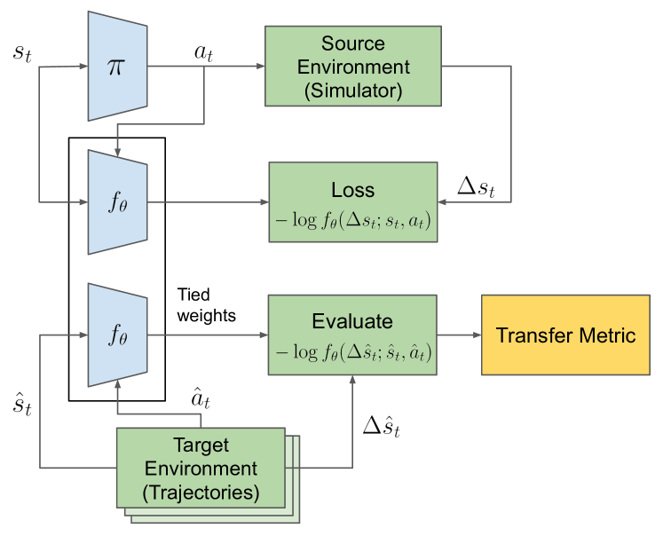
Figure 1: Transfer metric architecture. A probabilistic dynamics model is trained in the same source environment as the policy. The transfer metric is the average negative log-likelihood of the relative next state given by the model for trajectories from the target environment.

Several aspects of an environment may be predicted by the model: state, action, reward, and return (Irpan et al., 2019). We chose to predict the relative next state $\Delta s_{t}\triangleq s_{t+1}-s_{t}\in S^{\prime}$ from current state and action. We found relative state prediction to work better than absolute state prediction, which is consistent with prior work on training forward dynamics models (Deisenroth et al., 2015; Chua et al., 2018). A top-level diagram of the transfer metric is shown in Fig. 1.

We used a probabilistic forward dynamics model $f_{\theta}(\Delta s_{t};s_{t},a_{t})=P(\Delta s_{t}|s_{t},a_{t})$, where $\theta$ were the model parameters. For POMDPs, the inputs to the model were sequences of states and actions.

The prediction space $S^{\prime}$ was quantized to a set of discrete values. We found this helped model training significantly. The forward dynamics model was trained in the source environment using a negative log-likelihood (NLL) loss.

The transfer metric is the average NLL of the forward dynamics model evaluated on a set of pre-recorded trajectories from the target environment.

4 Experiments

4.1 Training Setup and Benchmark Tasks

Our experiments used the same policy and value function architectures as in (OpenAI et al., 2019). Each consisted of input embeddings, feed-forward layers, an LSTM core, and an output layer. PPO (Schulman et al., 2017) or SAC (Haarnoja et al., 2018a) with hindsight experience replay (HER) (Andrychowicz et al., 2017) was used for policy training.

We used the following benchmark dexterous in-hand manipulation tasks:

Block reorientation task

(OpenAI et al., 2018, 2019) requires the robot hand to orient a solid cube to match a goal orientation. Once the orientation matches, a successful rotation is declared and a new goal orientation is obtained. An episode continues until the robot hand either drops the cube or achieves 50 successful rotations.

Rubik’s cube task

(OpenAI et al., 2019) requires the robot to either rotate the top face of a Rubik’s cube by 90 degrees to match a goal face orientation or orient the entire Rubik’s cube to match a goal cube orientation. Here, we do not distinguish between face and cube rotations and declare a successful rotation when either occurs. The same episode termination conditions apply.

4.2 Simulator Randomizations

Domain randomization was used for policy training in simulation. The randomizations fall into two categories:

We apply parameter randomizations to environment parameters in the simulator. A calibration value is specified for a parameter, along with a fixed (in DR) or adjusted (in ADR) range centered at the calibration value. At the start of an episode, every randomized parameter is sampled uniformly from its range.

We additionally apply custom physics randomizations to incorporate real-world effects (such as motor backlash or action latency) into the simulation environment. We focus on five custom physics randomizations in particular: freezing cube, backlash, wind, action latency, and action noise.

Freezing cube randomly prevents the cube from being moved and is intended to model the dynamics of a cube stuck in some parts of the hand. Backlash models the motor backlash effect, as described in detail in (OpenAI et al., 2018). Wind models air flow around the cube. Action latency and noise are modifies how an action command from a policy is executed in simulation.

Each customs physics randomization involves some custom implementation of the physical dynamics with a set of parameters. A subset of these parameters are then randomized in a similar fashion as parameter randomization. For more details, see (OpenAI et al., 2018, 2019).

4.3 Sim-to-sim Transfer

In these experiments:

• Source Env: randomized simulation environments

• Target Env: held-out simulation environments

We used three parameter randomization methods in the held-out simulation environments:

• cal: always use the calibration value

• ext: uniformly sample the upper or lower limit of the parameter range

• rand: uniformly sample within the parameter range

We additionally used three different sets of custom physics randomizations in the held-out simulation environments:

• none: no custom physics

• partial: action latency, action noise

• all: freezing cube, backlash, wind, action latency, action noise

The set of all nine possible held-out environments given by is $\{\texttt{cal},\texttt{ext},\texttt{rand}\}\times\{\texttt{none},\texttt{partial},\texttt{all}\}$. We focused on the block reorientation task in these experiments. The source environments used for policy training is (rand, partial). Policy optimization was based on SAC with HER. We evaluated the prediction model on held-out environments directly to obtained the transfer metric. Fig. 2 shows a plot of the transfer metric and held-out performance.

The results show that the transfer metric predicts policy performance in a diverse set of held-out environments with strong linear correlation. It was also able to predict the effect of progressively adding more custom physics randomizations, for example the transfer metric increases quickly between (ext, none), (ext, partial), and (ext, all).

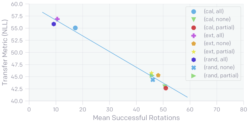
Figure 2: Transfer metric (NLL, lower is better) vs. performance in held-out environments. Training was performed in environments with (rand, partial) randomizations. The legend refers to the parameter and custom physics randomizations used in the held-out environment. The linear best-fit line has coefficient of determination of $R^{2}=-0.99$. Transfer metric strongly correlates with policy performance in held-out environments.

4.4 Sim-to-Real Transfer

In these experiments:

• Source Env: randomized simulation environments

• Target Env: physical Shadow robotic hand

We performed real-world deployments of policies for both the block reorientation task and the Rubik’s cube task. For block reorientation, we evaluated transfer metrics on a fixed set of trajectories recorded from Shadow robotic hands. They contains approximately 500 trajectories ranging from 20 to 3000 time steps. See Sec. 4.4.2 for details of the recorded trajectories used to evaluate the transfer metrics for the Rubik’s cube task.

4.4.1 Block Reorientation Policies

We picked three policies at different checkpoints of an ADR training run (‘Run 1’) for the block reorientation task. Fig. 3 shows the transfer metric and ADR entropy throughout the ADR training run. ADR entropy is the differential entropy of the environment distribution normalized by the number of environment parameters. It has been shown to correlate with real-world performance, where a higher ADR entropy is associated with better performance (OpenAI et al., 2019). As we show below, this is not true in general.

We picked the policies so that there is a large change in both transfer metric and ADR entropy between policies 1 and 2 but a nearly constant transfer metric between policies 2 and 3 while ADR entropy continues to increase.

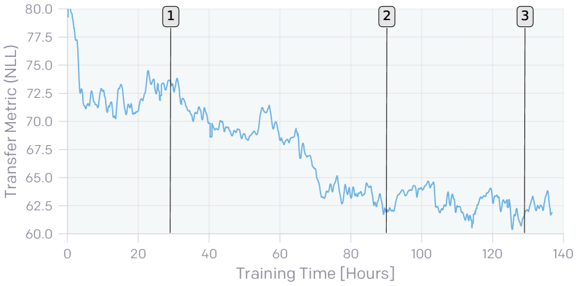
(a) Transfer Metric

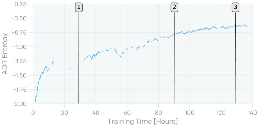
(b) ADR Entropy

Figure 3: Transfer metric and ADR entropy of ADR Run 1 for block reorientation. Policies were taken at the marked training times and deployed on a real robot. Missing segments in ADR entropy are due to an entropy value of -$\infty$. Note the decrease and flattening out of the transfer metric across the three policies in contrast to the constantly increasing ADR entropy.

We deployed the policies on a robotic hand by interleaving 5 episodes of each policy until 20 episodes have been collected for every policy. This procedure ensures that the robot condition is consistent across all policies. The results are shown in Table 1. For each ADR run (first column), the p-value is calculated using the two-sided, two-sample unequal variance t-test between the means of consecutive policies (with wrap-around), with the null hypothesis being equal means.

As expected, the results show a significant improvement in performance between policies 1 and 2. This is not surprising since both the transfer metric and ADR entropy changed significantly between these policies (not to mention the longer training time).

More interesting result is the small change in performance between policies 2 and 3. This is surprising when judged by ADR entropy or training time, which both increased between policies 2 and 3 and at the same rate as between policies 1 and 2. The transfer metric correctly predicted that performance will not continue to improve.

Table 1: Performance of block reorientation policies on robotic hand. Policies were trained under ADR with SAC. An ADR entropy of $-\infty$ corresponds to one or more components of the environment distribution being set to zero, see (OpenAI et al., 2019). ADR entropy is in units of nats-per-dimension (npd). For run 1, policy checkpoints refer to the markers in Fig. 3

			Number of successful rotations
Run	Policy Checkpoint	Time (days)	Transfer metric	ADR entropy	Mean	p-value
1	1	0.74	80.7	$-\infty$ npd	1.55	0.022
	2	3.8	61.6	$-0.78$ npd	3.35	0.54
	3	5.4	59.4	$-0.65$ npd	3.95	0.006
2	1	4.3	58.6	$-\infty$ npd	3.75	0.96
	2	5.5	58.8	$-0.51$ npd	3.70	0.96
3	1	2.5	73.7	$-\infty$ npd	1.90	0.094
	2	5.2	59.0	$-0.81$ npd	3.15	0.43
	3	5.8	63.0	$-0.73$ npd	2.55	0.26

As shown in Table 1, we repeated the above experiment for two additional ADR training runs: ‘Run 2’ and ‘Run 3’. The policies for ‘Run 2’ were picked to have essentially the same transfer metric ($58.6$ and $58.8$) but different ADR entropy. They are also separated in training time by more than a day. Performance of these policies on the robot were virtually identical.

The policies for ‘Run 3’ selected with a similar intention as ‘Run 1’. The difference here is that the transfer metric between policies 2 and 3 predicts a performance decrease while ADR entropy continues to increase. The results show that indeed, performance decreased from $3.15$ to $2.55$ mean successful rotations.

In summary, we showed in these experiments that the transfer metric is predictive of the block reorientation policy performance on a real-world robot. We further showed that the predictions cannot be explained by longer training times and are more accurate than ADR entropy.

4.4.2 Rubik’s Cube Policies

In these experiments, we study the sensitivity of the transfer metric to changes on the real-world robot. We performed 8 deployments of the same policy for the Rubik’s cube task. The policy was trained under ADR with PPO.

Deployments were performed on three different robotic hands, in two different state sensing setups (‘cages’) (OpenAI et al., 2019) and with varying amounts of mechanical and calibration degradation. The mean number of successful rotations of these deployments ranged from $4.3$ to $20.3$. Each deployment was recorded to be used for the transfer metric.

We evaluated a transfer metric for each deployment using its recorded trajectory. The results are shown in Fig. 4. We see that the transfer metric is able to predict the ordering of the performance on the robot.

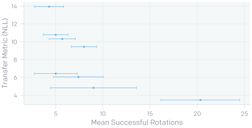
Figure 4: Performance and transfer metric of a single Rubik’s cube policy on different robotic hand setups (with different state-sensing setups and varying amounts of mechanical and calibration degradation). Error bars mark the standard error of the mean.

In summary, we showed in these experiments that the transfer metric is sensitive to changes in the robotic hand. We have shown this for the Rubik’s cube task, a much harder manipulation task than block reorientation.

4.4.3 Transfer Metrics of Existing Policies

In these experiments, we evaluated the transfer metric for policies that were deployed on the robotic hand and have available performance data. For each existing policy, we added a prediction model and performed rollouts in simulation. We optimized only the prediction model parameters using the rollout data. If ADR was used to train the policy, we also froze the ADR updates.

Table 2 shows the transfer metrics for existing block reorientation policies. The policies were originally trained under ADR with PPO or SAC. The transfer metrics were evaluated on the same block reorientation recordings as in the previous sections.

Table 2: Transfer metrics for existing block reorientation policies. The data contains a mix of policies trained with PPO or SAC under ADR. Different prediction architectures were used when training using PPO or SAC.

Policy	Algorithm	Transfer metric	Mean successful rotations
1	SAC	59.5	16.5
2	SAC	68.8	4.4
3	SAC	68.5	2.6
4	SAC	55.4	17.3
5	SAC	59.4	30.7
1	PPO	46.3	17.2
2	PPO	43.6	15.7
3	PPO	42.3	20.4

Good correlation is seen between the transfer metric and performance of existing block reorientation policies for the same algorithm.

Table 3 shows the transfer metrics for existing Rubik’s cube policies (OpenAI et al., 2019). These policies were trained using PPO under ADR. The transfer metrics were evaluated on the same Rubik’s cube recordings as in the previous sections.

Table 3: Transfer metrics for existing Rubik’s cube policies. ADR entropy is in units of nats-per-dimension (npd).

Policy	ADR entropy	Transfer metric	Mean successful rotations
1	$-0.054$ npd	73.6	3.8
2	$0.467$ npd	68.0	17.8
3	$0.479$ npd	67.2	26.8

Again, good correlation is seen between the transfer metric and performance of existing Rubik’s cube policies.

In summary, we showed in these experiments that it is not necessary to train the prediction model alongside the policy and that the transfer metric can be evaluated for existing policies. We also showed good correlation between the evaluate transfer metrics for existing both block reorientation and Rubik’s cube policies.

4.5 Transfer Metric and Domain Randomization

In these experiments:

• Source Env: randomized simulation environments

• Target Env: physical Shadow robotic hand

Here, we study the ability of the transfer metric to predict the effect of different levels of (fixed or automatic) domain randomization on policy transfer performance.

We trained block reorientation policies in Cal, DR, and ADR source environments. In the notation introduced in Sec. 4.3, the Cal source environment is (cal, full), where each parameter is fixed to a calibration value and all custom physics randomization are applied. The DR source environment is (rand, full), where each parameter is sampled uniformly from a fixed distribution and all custom physics randomizations are applied. The ADR source environment is the same as introduced in (OpenAI et al., 2019).

We evaluated the transfer metric on the set of trajectories given in Sec. 4.4. In these rollouts, the average performance of policies trained under Cal source environments is 2.5 mean successful rotations. Average performance for policies trained under DR source environments is 5.6 and under ADR source environments is 25.0. Therefore, the rollout data indicate that training under ADR is much better in terms of transfer performance than DR, which is still better than Cal.

Fig. 5 shows the transfer metric values for the three different sets of source environments. The transfer metric accurately predicts the relative ordering of average transfer performance of the resulting policies: $\texttt{ADR}>\texttt{DR}>\texttt{Cal}$.

We note that the initial dip in the ADR transfer metric is also present in the other two cases (only their time-averages are shown in Fig. 5). This is likely due to the initial randomly initialized policy does not change the observation state too much, hence the next state is trivial to predict.

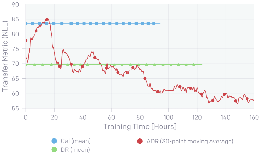
Figure 5: Transfer metric (NLL, lower is better) of different source environments. Transfer metrics for Cal and DR are averaged over the entire training run. Transfer metrics for ADR are smoothed by 30-point moving average. The transfer metric predicts the correct ordering of transfer performance: $\texttt{ADR}>\texttt{DR}>\texttt{Cal}$.

We also find that the ADR transfer metric evolves to first match the mean Cal transfer metric (after 18 hours of training), followed by the mean DR transfer metric (after 40 hours of training), then improves beyond both with additional training time. An explanation of this behaviour is that the environment distribution for ADR is initialized at the calibration environment, then automatically expands to approximate the manual DR distribution and beyond.

5 Conclusion

In this work, we proposed a method of predicting the real-world performance of policies trained in simulation, using only a fixed set of real-world trajectories. Our experiments showed that our transfer metric can successfully predict transfer performance in:

• Held-out simulation environments

• Real-world block reorientation with robotic hand

• Real-world Rubik’s cube with robotic hand

• Existing policies for block reorientation and Rubik’s cube

We also showed that our transfer metric can be used to select levels of domain randomization for best transfer performance and is an effective criterion for stopping ADR training.

References

- Andrychowicz et al. (2017) Andrychowicz, M., Wolski, F., Ray, A., Schneider, J., Fong, R., Welinder, P., McGrew, B., Tobin, J., Abbeel, P., and Zaremba, W. Hindsight Experience Replay. (NeurIPS), 2017. URL http://arxiv.org/abs/1707.01495.
- Chebotar et al. (2018) Chebotar, Y., Handa, A., Makoviychuk, V., Macklin, M., Issac, J., Ratliff, N., and Fox, D. Closing the Sim-to-Real Loop: Adapting Simulation Randomization with Real World Experience. CoRR, 2018. URL http://arxiv.org/abs/1810.05687.
- Christiano et al. (2016) Christiano, P., Shah, Z., Mordatch, I., Schneider, J., Blackwell, T., Tobin, J., Abbeel, P., and Zaremba, W. Transfer from Simulation to Real World through Learning Deep Inverse Dynamics Model. CoRR, 2016. URL https://arxiv.org/pdf/1610.03518.pdf.
- Chua et al. (2018) Chua, K., Calandra, R., McAllister, R., and Levine, S. Deep Reinforcement Learning in a Handful of Trials using Probabilistic Dynamics Models. (NeurIPS), 2018. URL http://arxiv.org/abs/1805.12114.
- Deisenroth et al. (2015) Deisenroth, M. P., Fox, D., and Rasmussen, C. E. Gaussian processes for data-efficient learning in robotics and control. IEEE Transactions on Pattern Analysis and Machine Intelligence, 37(2):408–423, 2015. ISSN 01628828.
- Farchy et al. (2013) Farchy, A., Barrett, S., MacAlpine, P., and Stone, P. Humanoid robots learning to walk faster: From the real world to simulation and back. International Conference on Autonomous Agents and Multi-Agent Systems (AAMAS’2013), (May):39–46, 2013. URL http://dl.acm.org/citation.cfm?id=2484930.
- Golemo et al. (2018) Golemo, F., Taïga, A. A., Oudeyer, P.-Y., and Courville, A. Sim-to-Real Transfer with Neural-Augmented Robot Simulation. In 2nd Conference on Robot Learning (CoRL18), Zurich, 2018. URL http://proceedings.mlr.press/v87/golemo18a/golemo18a.pdf.
- Haarnoja et al. (2018a) Haarnoja, T., Zhou, A., Abbeel, P., and Levine, S. Soft Actor-Critic: Off-Policy Maximum Entropy Deep Reinforcement Learning with a Stochastic Actor. CoRR, 2018a. URL http://arxiv.org/abs/1801.01290.
- Haarnoja et al. (2018b) Haarnoja, T., Zhou, A., Hartikainen, K., Tucker, G., Ha, S., Tan, J., Kumar, V., Zhu, H., Gupta, A., Abbeel, P., and Levine, S. Soft Actor-Critic Algorithms and Applications. CoRR, 2018b. URL http://arxiv.org/abs/1812.05905.
- Hanna & Stone (2017) Hanna, J. P. and Stone, P. Grounded Action Transformation for Robot Learning in Simulation. Conference on Artificial Intelligence (AAAI), (February):3834–3840, 2017.
- Hwangbo et al. (2019) Hwangbo, J., Koltun, V., Tsounis, V., Hutter, M., Bellicoso, D., Lee, J., and Dosovitskiy, A. Learning agile and dynamic motor skills for legged robots. Science Robotics, 4(26), 2019.
- Irpan et al. (2019) Irpan, A., Rao, K., Bousmalis, K., Harris, C., Ibarz, J., and Levine, S. Off-Policy Evaluation via Off-Policy Classification. CoRR, Jun 2019. URL http://arxiv.org/abs/1906.01624.
- Koos et al. (2010) Koos, S., Mouret, J.-B., and Doncieux, S. Crossing the Reality Gap in Evolutionary Robotics by Promoting Transferable Controllers. In GECCO10, Portland, 2010. ACM. URL http://www.isir.upmc.fr/files/2010ACTI1527.pdf.
- Mehta et al. (2019) Mehta, B., Diaz, M., Golemo, F., Pal, C. J., and Paull, L. Active Domain Randomization. In 3rd Conference on Robot Learning (CoRL19), 2019. URL http://arxiv.org/abs/1904.04762.
- Muratore et al. (2018) Muratore, F., Treede, F., Gienger, M., and Peters, J. Domain Randomization for Simulation-Based Policy Optimization with Transferability Assessment. In 2nd Conference on Robot Learning (CoRL 2018), Zurich, 2018.
- OpenAI et al. (2018) OpenAI, Andrychowicz, M., Baker, B., Chociej, M., Józefowicz, R., McGrew, B., Pachocki, J., Petron, A., Plappert, M., Powell, G., Ray, A., Schneider, J., Sidor, S., Tobin, J., Welinder, P., Weng, L., and Zaremba, W. Learning Dexterous In-Hand Manipulation. CoRR, 2018. URL https://arxiv.org/pdf/1808.00177.pdf.
- OpenAI et al. (2019) OpenAI, Akkaya, I., Andrychowicz, M., Chociej, M., Litwin, M., McGrew, B., Petron, A., Paino, A., Plappert, M., Powell, G., Ribas, R., Schneider, J., Tezak, N., Tworek, J., Welinder, P., Weng, L., Yuan, Q., Zaremba, W., and Zhang, L. Solving Rubik’s Cube with a Robot Hand. CoRR, 2019. URL https://arxiv.org/pdf/1910.07113.pdf.
- Pashevich et al. (2019) Pashevich, A., Strudel, R. A. M., Kalevatykh, I., Laptev, I., and Schmid, C. Learning to Augment Synthetic Images for Sim2Real Policy Transfer. CoRR, 2019. URL http://arxiv.org/abs/1903.07740.
- Peng et al. (2018) Peng, X. B., Andrychowicz, M., Zaremba, W., and Abbeel, P. Sim-to-Real Transfer of Robotic Control with Dynamics Randomization. 2018. URL https://arxiv.org/pdf/1710.06537.pdf.
- Prakash et al. (2018) Prakash, A., Boochoon, S., Brophy, M., Acuna, D., Cameracci, E., State, G., Shapira, O., and Birchfield, S. Structured Domain Randomization: Bridging the Reality Gap by Context-Aware Synthetic Data. CoRR, Oct 2018. URL http://arxiv.org/abs/1810.10093.
- Rusu et al. (2016) Rusu, A. A., Vecerik, M., Rothörl, T., Heess, N., Pascanu, R., and Hadsell, R. Sim-to-Real Robot Learning from Pixels with Progressive Nets. CoRR, 2016. URL http://arxiv.org/abs/1610.04286.
- Sadeghi & Levine (2017) Sadeghi, F. and Levine, S. CAD2RL: Real Single-Image Flight without a Single Real Image. CoRR, 2017. URL http://arxiv.org/abs/1611.04201.
- Schulman et al. (2017) Schulman, J., Wolski, F., Dhariwal, P., Radford, A., and Klimov, O. Proximal Policy Optimization Algorithms. CoRR, Jul 2017. URL https://arxiv.org/abs/1707.06347.
- Tan et al. (2018) Tan, J., Zhang, T., Coumans, E., Iscen, A., Bai, Y., Hafner, D., Bohez, S., and Vanhoucke, V. Sim-to-Real: Learning Agile Locomotion For Quadruped Robots. CoRR, 2018. URL http://arxiv.org/abs/1804.10332.
- Tobin et al. (2017) Tobin, J., Fong, R., Ray, A., Schneider, J., Zaremba, W., and Abbeel, P. Domain Randomization for Transferring Deep Neural Networks from Simulation to the Real World. CoRR, 2017. URL https://arxiv.org/pdf/1703.06907.pdf.
- Todorov et al. (2012) Todorov, E., Erez, T., and Tassa, Y. MuJoCo: A physics engine for model-based control. 2012 IEEE/RSJ International Conference on Intelligent Robots and Systems, pp. 5026–5033, 2012.