Radially and azimuthally excited states of a soliton system of vortex and Q-ball

Abstract

In the present paper, we continue to study the two-dimensional soliton system that is composed of vortex and Q-ball components interacting with each other through an Abelian gauge field. This vortex-Q-ball system is electrically neutral as a whole, nevertheless it possesses a nonzero electric field. Moreover, the vortex-Q-ball system has a quantized magnetic flux and a nonzero angular momentum, and combines properties of topological and nontopological solitons. We investigate radially and azimuthally excited states of the vortex-Q-ball system along with the unexcited vortex-Q-ball system at different values of gauge coupling constants. We also ascertain the behaviour of the vortex-Q-ball system in several extreme regimes, including thin-wall and thick-wall regimes.

1 Introduction

It is known that $(1+1)$-dimensional gauge models and $(2+1)$-dimensional gauge models without the Chern-Simons term do not allow the existence of electrically charged solitons because any electrically charged compact object will have infinite energy in these models. The reason for this is simple: at large distances, the electric field of a one-dimensional object does not depend on the distance and that of a two-dimensional object is inversely proportional to the distance. As a result, with increasing distance, the energy of the electric field diverges linearly in the one-dimensional case and logarithmically in the two-dimensional case.

The electrically charged solitons appear only in $(3+1)$-dimensional gauge models (e.g. the three-dimensional electrically charged dyon julia_zee or Q-ball rosen ; klee ; anag ; ardoz_2009 ; tamaki_2014 ; gulamov_2014 ). Note, however, that the Chern-Simons term can be added to the Lagrangian of a $(2+1)$-dimensional gauge model. Moreover, $(2+1)$-dimensional gauge models may be pure Chern-Simons, and hence have no Maxwell gauge term. Such $(2+1)$-dimensional gauge models may admit the existence of electrically charged solitons. Indeed, electrically charged vortices were found in both the pure Chern-Simons hong ; jw1 ; jw2 ; bazeia_1991 ; ghosh and the Maxwell-Chern-Simons paul ; khare_rao_227 ; khare_255 ; loginov_plb_784 gauge models. In addition, one-dimensional domain walls may exist in Chern-Simons gauge models dsantos ; losano . These Chern-Simons domain walls possess finite linear densities of energy, magnetic flux, and electric charge.

Thus, in $(1+1)$ and $(2+1)$-dimensional pure Maxwell gauge models, solitons should be electrically neutral. The neutrality, however, does not mean the absence of electric field. In Refs. loginov_plb_777 ; loginov_epj_79 , one and two-dimensional soliton systems composed of topological and nontopological components were described. The components interact with each other through an Abelian gauge field and possess opposite electric charges, so the soliton systems are neutral as a whole. Despite electrical neutrality, these soliton systems possess a nonzero electric field that tends to zero exponentially at spatial infinity, resulting in finite electrostatic energy.

The characteristic feature of nontopological solitons is the presence of radially and azimuthally excited states FLS_1976 ; volkov_prd_66 ; kunz_prd_72 ; mai_prd_86 ; loginov_prd_102 . The Q-ball components of compound soliton systems may also be radially or azimuthally excited. The corresponding excited compound soliton systems will have some new features compared to unexcited systems. In the present paper, we study radially and azimuthally excited states of the vortex-Q-ball soliton system described in loginov_plb_777 . We also study the unexcited vortex-Q-ball system using different values of gauge coupling constants.

The paper is structured as follows. In Sect. 2, we describe the Lagrangian, the symmetries, the field equations, and the energy-momentum tensor of the gauge model under consideration. In Sect. 3, we list some properties of the vortex-Q-ball system; among them, the basic differential relation, the asymptotic behaviour of fields at small and large distances, some properties of the gauge potential, the virial relation, and the Laue condition for the vortex-Q-ball system. In Sect. 4, we study properties of the vortex-Q-ball system at extreme values of parameters. In Sect. 5, we present and discuss the numerical results for the unexcited vortex-Q-ball system at different values of gauge coupling constants, the radially excited vortex-Q-ball system, and the azimuthally excited vortex-Q-ball system. In all three cases, we present dependences of the vortex-Q-ball energy on the phase frequency and on the Noether charge along with radial dependences of the vortex-Q-ball ansatz functions.

Throughout the paper, we use the natural units $\hbar=c=1$.

2 The gauge model

The Lagrangian density of the $\left(2+1\right)$-dimensional gauge model under consideration has the form

$$\mathcal{L} = -\frac{1}{4}F_{\mu\nu}F^{\mu\nu}+\left(D_{\mu}\phi\right)^{\ast}D^{\mu}\phi-V\left(\left|\phi\right|\right)$$ (1)

$$+\left(D_{\mu}\chi\right)^{\ast}D^{\mu}\chi-U\left(\left|\chi\right|\right).$$

The model describes the two complex scalar fields $\phi$ and $\chi$ that minimally interact with the Abelian gauge field $A_{\mu}$ through the covariant derivatives

$$D_{\mu}\phi=\partial_{\mu}\phi+ieA_{\mu}\phi,\quad D_{\mu}\chi=\partial_{\mu}\chi+iqA_{\mu}\chi.$$ (2)

The scalar fields $\phi$ and $\chi$ are self-interacting ones. The self-interaction of $\phi$ and $\chi$ is described by the fourth- and sixth-order potentials, respectively

$$V\left(\left|\phi\right|\right) = \frac{\lambda}{2}\left(\left|\phi\right|^{2}-v^{2}\right)^{2},$$ (3a)

$$U\left(\left|\chi\right|\right) = m^{2}\left|\chi\right|^{2}-\frac{g}{2}\left|\chi\right|^{4}+\frac{h}{3}\left|\chi\right|^{6},$$ (3b)

where $\left|\phi\right|^{2}=\phi^{\ast}\phi$ and $\left|\chi\right|^{2}=\chi^{\ast}\chi$. In Eqs. (3a) and (3b), $\lambda$, $g$, and $h$ are positive self-interaction constants, $m$ is the mass of the scalar $\chi$-particle, and $v$ is the vacuum average of the amplitude of the complex scalar field $\phi$. From Eq. (3a) it follows that the potential $V\left(\left|\phi\right|\right)$ possesses the continuous family of minima lying on the circle $\left|\phi\right|=v$. At the same time, we suppose that the potential $U\left(\left|\chi\right|\right)$ has a global isolated minimum at $\chi=0$. For this to hold, the parameters of $U\left(\left|\chi\right|\right)$ must satisfy the inequality $3g^{2}<16m^{2}h$.

The invariance of the Lagrangian density (1) under local gauge transformations

$$\phi\left(x\right) \rightarrow \phi^{\prime}\left(x\right)=\exp\left(-ie\Lambda\left(x\right)\right)\phi\left(x\right),$$

$$\chi\left(x\right) \rightarrow \chi^{\prime}\left(x\right)=\exp\left(-iq\Lambda\left(x\right)\right)\chi\left(x\right),$$

$$A_{\mu}\left(x\right) \rightarrow A_{\mu}^{\prime}\left(x\right)=A_{\mu}\left(x\right)+\partial_{\mu}\Lambda\left(x\right)$$ (4)

and the electrical neutrality of the Abelian gauge field $A_{\mu}$ lead to the invariance of the model under the two independent global gauge transformations

$$\phi\left(x\right) \rightarrow \phi^{\prime}\left(x\right)=\exp\left(-i\alpha\right)\phi\left(x\right),$$

$$\chi\left(x\right) \rightarrow \chi^{\prime}\left(x\right)=\exp\left(-i\beta\right)\chi\left(x\right).$$ (5)

The invariance of the Lagrangian density under global transformations (5) results in the existence of the two conserved Noether currents

$$j_{\phi}^{\mu} = i\left[\phi^{\ast}D^{\mu}\phi-\left(D^{\mu}\phi\right)^{\ast}\phi\right],$$

$$j_{\chi}^{\mu} = i\left[\chi^{\ast}D^{\mu}\chi-\left(D^{\mu}\chi\right)^{\ast}\chi\right].$$ (6)

The field equations for the model have the form

$$D_{\mu}D^{\mu}\phi+\lambda\left(\left|\phi\right|^{2}-v^{2}\right)\phi = 0,$$ (7)

$$D_{\mu}D^{\mu}\chi+m^{2}\chi-g\left|\chi\right|^{2}\chi+h\left|\chi\right|^{4}\chi = 0,$$ (8)

$$\partial_{\mu}F^{\mu\nu} = j^{\nu},$$ (9)

where the electromagnetic current $j^{\nu}$ is

$$j^{\nu} = ej_{\phi}^{\mu}+qj_{\chi}^{\mu}$$

$$= ie\phi^{\ast}\overleftrightarrow{\partial^{\nu}}\phi-2e^{2}A^{\nu}\phi^{\ast}\phi+iq\chi^{\ast}\overleftrightarrow{\partial^{\nu}}\chi-2q^{2}A^{\nu}\chi^{\ast}\chi.$$

In Sect. 3, we shall need the form of the symmetric energy-momentum tensor $T_{\mu\nu}$ of the model

$$T_{\mu\nu} = 2\partial\mathcal{L}/\partial g^{\mu\nu}-g_{\mu\nu}\mathcal{L}$$ (11)

$$=-F_{\mu\lambda}F_{\nu}^{\;\lambda}+\frac{1}{4}g_{\mu\nu}F_{\lambda\rho}F^{\lambda\rho}$$

$$+\left(D_{\mu}\phi\right)^{\ast}D_{\nu}\phi+\left(D_{\nu}\phi\right)^{\ast}D_{\mu}\phi$$

$$-g_{\mu\nu}\left(\left(D_{\mu}\phi\right)^{\ast}D^{\mu}\phi-V\left(\left|\phi\right|\right)\right)$$

$$+\left(D_{\mu}\chi\right)^{\ast}D_{\nu}\chi+\left(D_{\nu}\chi\right)^{\ast}D_{\mu}\chi$$

$$-g_{\mu\nu}\left(\left(D_{\mu}\chi\right)^{\ast}D^{\mu}\chi-U\left(\left|\chi\right|\right)\right).$$

In particular, we shall need the expression for the energy density $\mathcal{E}=T_{00}$ of a field configuration of the model

$$\mathcal{E} = \frac{1}{2}E_{i}E_{i}+\frac{1}{2}B^{2}$$ (12)

$$+\left(D_{0}\phi\right)^{\ast}D_{0}\phi+\left(D_{i}\phi\right)^{\ast}D_{i}\phi+V\left(\left|\phi\right|\right)$$

$$+\left(D_{0}\chi\right)^{\ast}D_{0}\chi+\left(D_{i}\chi\right)^{\ast}D_{i}\chi+U\left(\left|\chi\right|\right),$$

where $E_{i}=F_{0i}$ and $B=F_{21}$ are the electric field strength and the magnetic field strength, respectively.

3 The vortex-Q-ball soliton system and some of its properties

When the gauge coupling constant $q$ is equal to zero, model (1) possesses both the ANO vortex solution abrikosov ; nielsen formed of the complex scalar field $\phi$ and the gauge field $A_{\mu}$ and the two-dimensional nongauged $Q$-ball solution formed of the complex scalar field $\chi$. The ANO vortex and the two-dimensional $Q$-ball are electrically neutral, thus they do not interact with each other. The situation changes drastically if the gauge coupling constant $q$ is different from zero. It was shown in Ref. loginov_plb_777 that in this case, the soliton system consists of interacting vortex and $Q$-ball components. This two-dimensional vortex-Q-ball system is electrically neutral as a whole, because its vortex and $Q$-ball components have opposite electrical charges. Nevertheless, the vortex-Q-ball system possesses a nonzero radial electric field in its interior.

Using the Hamilton formalism and Lagrange’s method of multipliers FLS_1976_2 ; FLS_1976_3 , it was shown in Ref. loginov_plb_777 that there exists a gauge in which only the complex scalar field $\chi$ has nontrivial time dependence $\propto\exp\left[-i\omega t\right]$, while the complex scalar field $\phi$ and the Abelian gauge field $A_{\mu}$ do not depend on time. It was also shown that the vortex-Q-ball system satisfies the important differential relation

$$\frac{dE}{dQ_{\chi}}=\omega,$$ (13)

where $E=\int\mathcal{E}d^{2}x$ and $Q_{\chi}=\int j_{\chi}^{0}d^{2}x$ are the energy and the Noether charge of the vortex-Q-ball system, respectively, and $\omega$ is the phase frequency of the complex scalar field $\chi$. Note that in Eq. (13), the phase frequency $\omega$ is treated as a function of the Noether charge $Q_{\chi}$. Eq. (13) is a consequence of the fact that the vortex-Q-ball system is an extremum of the energy functional $E=\int\mathcal{E}d^{2}x$ at a fixed value of the Noether charge $Q_{\chi}=\int j_{\chi}^{0}d^{2}x$.

To describe the vortex-Q-ball system, we shall use the following ansatz

$$\phi\left(r,\theta\right) = v\exp\left(iN\theta\right)F\left(r\right),$$ (14a)

$$\chi\left(r,\theta,t\right) = \exp\left[-i\left(\omega t-K\theta\right)\right]\sigma\left(r\right),$$ (14b)

$$A^{\mu}\left(r,\theta\right) = \left(\frac{a_{0}\left(r\right)}{er},\frac{1}{er}\epsilon_{ij}n_{j}a\left(r\right)\right),$$ (14c)

where $K$ and $N$ are integers, $\epsilon^{ij}$ are the components of the two-dimensional antisymmetric tensor ($\epsilon^{12}=1$) and $n_{j}$ are those of the two-dimensional radial unit vector $\mathbf{n}=(\cos(\theta),\sin(\theta))$. The ansatz functions $a_{0}\left(r\right)$, $a\left(r\right)$, $F\left(r\right)$, and $\sigma\left(r\right)$ satisfy the system of nonlinear differential equations

$$a_{0}^{\prime\prime}(r)-\frac{a_{0}^{\prime}(r)}{r}+\frac{a_{0}(r)}{r^{2}}-2e^{2}v^{2}F\left(r\right)^{2}a_{0}(r)$$

$$+2eqr\left[\omega-\frac{q}{e}\frac{a_{0}(r)}{r}\right]\sigma\left(r\right)^{2}=0,$$ (15)

$$a^{\prime\prime}(r)-\frac{a^{\prime}(r)}{r}-2e^{2}v^{2}\left(N+a(r)\right)F\left(r\right)^{2}$$

$$-2eq\left[K+\frac{q}{e}a\left(r\right)\right]\sigma\left(r\right)^{2}=0,$$ (16)

$$F^{\prime\prime}(r)+\frac{F^{\prime}(r)}{r}-\frac{\left((N+a(r))^{2}-a_{0}(r)^{2}\right)}{r^{2}}F(r)$$

$$+\lambda v^{2}\left(1-F(r)^{2}\right)F(r)=0,$$ (17)

$$\sigma^{\prime\prime}(r)+\frac{\sigma^{\prime}(r)}{r}+\left[\left(\omega-\frac{q}{e}\frac{a_{0}\left(r\right)}{r}\right)^{2}\right.$$

$$-\left.\left(\frac{K}{r}+\frac{q}{e}\frac{a\left(r\right)}{r}\right)^{2}\right]\sigma\left(r\right)$$

$$-\left(m^{2}-g\sigma\left(r\right)^{2}+h\sigma\left(r\right)^{4}\right)\sigma\left(r\right)=0.$$ (18)

The energy density of the vortex-Q-ball system can also be expressed in terms of the ansatz functions

$$\mathcal{E} \mathcal{=} \frac{1}{2}\frac{a^{\prime}{}^{2}}{e^{2}r^{2}}+\frac{1}{2}\left[\left(\frac{a_{0}}{er}\right)^{\prime}\right]^{2}$$ (19)

$$+v^{2}F^{\prime}{}^{2}+\frac{\left((N+a)^{2}+a_{0}{}^{2}\right)}{r^{2}}v^{2}F^{2}$$

$$+\frac{\lambda}{2}v^{4}\left(F^{2}-1\right)^{2}+\sigma^{\prime}{}^{2}$$

$$+\left(\omega-\frac{q}{e}\frac{a_{0}}{r}\right)^{2}\sigma^{2}+\left(\frac{K}{r}+\frac{q}{e}\frac{a}{r}\right)^{2}\sigma^{2}$$

$$+m^{2}\sigma^{2}-\frac{g}{2}\sigma^{4}+\frac{h}{3}\sigma^{6}.$$

The regularity of the vortex-Q-ball solution at $r=0$ and the finiteness of the energy $E=2\pi\int\nolimits_{0}^{\infty}\mathcal{E}\left(r\right)rdr$ lead to the boundary conditions for the ansatz functions

$$\;a_{0}(0)=0,\;\underset{r\rightarrow\infty}{\lim}a_{0}(r)=0,$$ (20a)

$$\;a(0)=0,\;\underset{r\rightarrow\infty}{\lim}a(r)=-N,$$ (20b)

$$\;F(0)=0,\;\underset{r\rightarrow\infty}{\lim}F(r)=1,$$ (20c)

$$\;\delta_{K0}\sigma^{\prime}(0)+\left(1-\delta_{K0}\right)\sigma(0)=0,\;\underset{r\rightarrow\infty}{\lim}\sigma(r)=0,$$ (20d)

where $\delta_{K0}$ is the Kronecker symbol.

Substituting the power expansions for the ansatz functions in Eqs. (15)–(18) and taking into account boundary conditions (20), we obtain the power expansion at the origin of the vortex-Q-ball solution with $N=1$. The power expansion of the ansatz function $a_{0}\left(r\right)$ has the form

$$a_{0}\left(r\right)=a_{1}r+\frac{a_{p}}{p!}r^{p}+O\left(r^{p+2}\right),$$ (21)

where

$$p=3\delta_{K0}+5\left(1-\delta_{K0}\right)$$ (22)

and

$$a_{3} = 3qd_{0}^{2}\left(a_{1}q-e\omega\right),$$ (23a)

$$a_{5} = 15e^{2}v^{2}a_{1}c_{1}^{2}+15\delta_{\left|K\right|\,1}\left(d_{1}^{2}q\left(a_{1}q-e\omega\right)\right).$$ (23b)

The power expansions of the ansatz functions $a\left(r\right)$ and $F\left(r\right)$ are written as

$$a\left(r\right) = \frac{b_{2}}{2!}r^{2}+\frac{b_{4}}{4!}r^{4}+O\left(r^{6}\right),$$ (24)

$$F\left(r\right) = c_{1}r+\frac{c_{3}}{3!}r^{3}+O\left(r^{5}\right),$$ (25)

where the next-to-leading order coefficients are

$$b_{4} = 6e^{2}v^{2}c_{1}^{2}+3\delta_{K0}q^{2}b_{2}d_{0}^{2}+6\text{sgn}\left(K\right)\delta_{\left|K\right|\,1}eqd_{1}^{2},$$ (26)

$$c_{3} = -\frac{3}{4}c_{1}\left(a_{1}^{2}-b_{2}+\lambda v^{2}\right).$$ (27)

Finally, the power expansion of the ansatz function $\sigma\left(r\right)$ is

$$\sigma\left(r\right)=\frac{d_{\left|K\right|}}{\left|K\right|!}r^{\left|K\right|}+\frac{d_{\left|K\right|+2}}{\left(\left|K\right|+2\right)!}r^{\left|K\right|+2}+O\left(r^{\left|K\right|+4}\right),$$ (28)

where the next-to-leading order coefficient is

$$d_{\left|K\right|+2} = \frac{\left|K\right|+2}{4e^{2}}\left[\left(e\left(m+\omega\right)-qa_{1}\right)\right.$$ (29)

$$\times\left.\left(e\left(m-\omega\right)+qa_{1}\right)+\tau_{K}\right]d_{\left|K\right|}$$

and the term $\tau_{K}$ is

$$\tau_{K}=-e^{2}d_{0}^{2}\left(2g-3hd_{0}^{2}\right)\delta_{K0}+eqKb_{2}\left(1-\delta_{K0}\right).$$ (30)

To obtain the asymptotic form of the vortex-Q-ball solution as $r\rightarrow\infty$, we linearize Eqs. (15)–(18) and use boundary conditions (20). As a result, we obtain the expressions

$$a_{0}\left(r\right) \sim a_{\infty}\sqrt{m_{A}r}\exp\left(-m_{A}r\right)$$ (31)

$$\times\left(1-\frac{1}{8m_{A}r}+O\left[\left(\frac{1}{m_{A}r}\right)^{2}\right]\right),$$

$$a\left(r\right) \sim N+b_{\infty}\sqrt{m_{A}r}\exp\left(-m_{A}r\right)$$ (32)

$$\times\left(1+\frac{3}{8m_{A}r}+O\left[\left(\frac{1}{m_{A}r}\right)^{2}\right]\right),$$

$$F\left(r\right) \sim 1+c_{\infty}\frac{\exp\left(-m_{\phi}r\right)}{\sqrt{m_{\phi}r}}$$ (33)

$$\times\left(1-\frac{1}{8m_{\phi}r}+O\left[\left(\frac{1}{m_{\phi}r}\right)^{2}\right]\right),$$

$$\sigma\left(r\right) \sim d_{\infty}\frac{\exp\left(-\Delta_{\omega}r\right)}{\sqrt{\Delta_{\omega}r}}\left(1+\frac{4\left(K-qN/e\right)^{2}-1}{8\Delta_{\omega}r}\right.$$ (34)

$$\left.+O\left[\left(\frac{1}{\Delta_{\omega}r}\right)^{2}\right]\right),$$

where $m_{A}=\sqrt{2}ev$ and $m_{\phi}=\sqrt{2\lambda}v$ are the masses of the gauge boson and the scalar $\phi$-particle, respectively, and $\Delta_{\omega}=\sqrt{m^{2}-\omega^{2}}$ is the mass parameter that defines the asymptotic behaviour of the scalar field $\chi$. Note that the asymptotic forms (31)–(34) are valid only if the mass of any of the three particles (gauge boson, $\phi$-particle, and $\chi$-particle) does not exceed the sum of the mass of the two remaining particles, with the mass parameter $\Delta_{\omega}$ playing the role of the $\chi$-particle’s mass. Only if this condition is met, can Eqs. (15)–(18) be linearised.

From Eqs. (21)–(30), it follows that the behaviour of the vortex-Q-ball solution in the neighbourhood of $r=0$ is determined by four independent parameters: $a_{1}$, $b_{2}$, $c_{1}$, and $d_{K}$. At the same time, Eqs. (31)–(34) tell us that the behaviour of the vortex-Q-ball solution at spatial infinity is also determined by four independent parameters: $a_{\infty}$, $b_{\infty}$, $c_{\infty}$, and $d_{\infty}$. The coincidence of the numbers of parameters that define the behaviour of the solution at the origin and at infinity makes the existence of a solution of the boundary value problem in Eqs. (15)–(18) and (20) possible.

Having boundary conditions (20), we can obtain the constraint on the Noether charges $Q_{\phi}$ and $Q_{\chi}$ of the vortex-Q-ball system. To do this, we rewrite Eq. (15) (Gauss’s law) in compact form

$$\left[r\left(\frac{a_{0}(r)}{er}\right)^{\prime}\right]^{\prime}=-rj_{0}\left(r\right),$$ (35)

where $j_{0}\left(r\right)$ is the electric charge density expressed in terms of the ansatz functions

$$j_{0} = 2q\omega\sigma\left(r\right)^{2}-\frac{2a_{0}\left(r\right)}{er}\left(q^{2}\sigma\left(r\right)^{2}+e^{2}v^{2}F\left(r\right)^{2}\right)\!.$$ (36)

Then, we integrate both sides of Eq. (35) with respect to $r$ from zero to infinity. Using boundary conditions (20) and asymptotic expressions (21)–(30) and (31)–(34) of the vortex-Q-ball solution, it is easily shown that the integral of the left-hand side of Eq. (35) vanishes. At the same time, the integral of the right-hand side of Eq. (35) is proportional to the electric charge of the vortex-Q-ball system. It follows that the electric charge of the vortex-Q-ball system vanishes. Combining this fact and Eq. (2), we obtain the constraint on the Noether charges $Q_{\phi}$ and $Q_{\chi}$ of the vortex-Q-ball system

$$Q=eQ_{\phi}+qQ_{\chi}=0,$$ (37)

where the Noether charges are expressed in terms of the ansatz functions

$$Q_{\phi} = -4\pi v^{2}\int\limits_{0}^{\infty}a_{0}\left(r\right)F\left(r\right)^{2}dr,$$ (38a)

$$Q_{\chi} = 4\pi\int\limits_{0}^{\infty}\left(\omega-\frac{q}{e}\frac{a_{0}\left(r\right)}{r}\right)\sigma\left(r\right)^{2}rdr.$$ (38b)

Gauss’s law (15) allows us to ascertain some global properties of the time component of the gauge potential $A_{0}(r)=a_{0}(r)/(er)$. To do this, we rewrite Eq. (15) in the form

$$\left(r\Omega^{\prime}\left(r\right)\right)^{\prime}=2r\left[q^{2}\sigma\left(r\right)^{2}\Omega\left(r\right)-e^{2}v^{2}F\left(r\right)^{2}\left(\omega-\Omega\left(r\right)\right)\right],$$ (39)

where the function

$$\Omega\left(r\right)=\omega-qA_{0}(r)=\omega-\frac{q}{e}\frac{a_{0}\left(r\right)}{r}.$$ (40)

According to Eq. (20a), the function $\Omega\left(r\right)\rightarrow\omega$ as $r\rightarrow\infty$. Let the phase frequency $\omega$ be positive, then from Eq. (39) it follows that $0<\Omega\left(r\right)<\omega$. Indeed, if $\Omega\left(r\right)<0$ $\left(\Omega\left(r\right)>\omega\right)$ at some $r=\bar{r}$, then $\Omega^{\prime}\left(r\right)$ will be negative (positive) at $r>\bar{r}$, and thus the boundary condition $\Omega\left(r\right)\underset{r\rightarrow\infty}{\rightarrow}\omega$ cannot be satisfied. If the phase frequency $\omega$ is negative, then $\omega<\Omega\left(r\right)<0$. Thus, we have the global conditions on $\Omega\left(r\right)$

$$0 < \Omega\left(r\right)<\omega\;\text{if}\;\omega>0,$$

$$\omega < \Omega\left(r\right)<0\;\text{if}\;\omega<0,$$ (41)

which can be rewritten in terms of the gauge potential $A_{0}(r)=a_{0}(r)/(er)$ as

$$0 < A_{0}\left(r\right)<\frac{\omega}{q}\;\text{if}\;\omega>0,$$

$$\frac{\omega}{q} < A_{0}\left(r\right)<0\;\text{if}\;\omega<0.$$ (42)

Eq. (20b) tells us that the boundary conditions for the ansatz function $a\left(r\right)$ are the same as those for the ANO vortex. It follows that the magnetic flux of the vortex-Q-ball system is quantized as it is for the ANO vortex

$$\Phi=2\pi\int\limits_{0}^{\infty}B\left(r\right)rdr=\frac{2\pi}{e}N,$$ (43)

where $B(r)=-a^{\prime}(r)/(er)$ is the magnetic field strength. In particular, the magnetic flux of the vortex-Q-ball system does not depend on the gauge coupling constant $q$ that determines the strength of interaction between the gauge field $A_{\mu}$ and the complex scalar field $\chi$.

Having the symmetric energy-momentum tensor (11), we can form the angular momentum tensor

$$J^{\lambda\mu\nu}=x^{\mu}T^{\lambda\nu}-x^{\nu}T^{\lambda\mu}.$$ (44)

Use of Eqs. (11), (14), and (44) results in the angular momentum density $\mathcal{J}=\frac{1}{2}\epsilon_{ij}J^{0ij}=J^{012}$ expressed in terms of the ansatz functions

$$\mathcal{J} = -rBE_{r}+2\left(K+\frac{q}{e}a\right)\left(\omega-\frac{q}{e}\frac{a_{0}}{r}\right)\sigma^{2}$$ (45)

$$-2\frac{a_{0}\left(N+a\right)}{r}v^{2}F^{2},$$

where $E_{r}(r)=-\left(a_{0}\left(r\right)/\left(er\right)\right)^{\prime}$ is the radial electric field strength. Next, we integrate the term $-rBE_{r}=-e^{-2}a^{\prime}\left(a_{0}/r\right)^{\prime}$ by parts, taking into account boundary conditions (20) and using Gauss’s law (15) to eliminate $a_{0}^{\prime\prime}$. As a result, the expression for the angular momentum $J=2\pi\int\nolimits_{0}^{\infty}\mathcal{J}\left(r\right)rdr$ of the vortex-Q-ball system takes the form

$$J = -4\pi N\int\limits_{0}^{\infty}v^{2}a_{0}\left(r\right)F\left(r\right)^{2}dr$$ (46)

$$+4\pi K\int\limits_{0}^{\infty}r\left(\omega-\frac{q}{e}\frac{a_{0}\left(r\right)}{r}\right)\sigma\left(r\right)^{2}dr$$

$$= NQ_{\phi}+KQ_{\chi},$$

where the last line in Eq. (46) follows from Eqs. (38a) and (38b). Using Eq. (37), we can rewrite Eq. (46) in two equivalent forms

$$J=\left(K-\frac{q}{e}N\right)Q_{\chi}=\left(N-\frac{e}{q}K\right)Q_{\phi}.$$ (47)

Let suppose that the gauge coupling constants $e$ and $q$ are multiples of some minimal gauge coupling constant, then the ratio $q/e$ is a rational number. Eq. (47) tells us that in this case, the angular momentum of the vortex-Q-ball system vanishes when the ratio $K/N$ is equal to $q/e$. Conversely, the ratio $q/e$ is a rational number if there exists a vortex-Q-ball system possessing zero angular momentum. Note that if $K/N=q/e$ then field configuration (14) is invariant under an axial rotation modulo the corresponding gauge transformation, as it should be for a gauged soliton system possessing zero angular momentum.

Using Eqs. (15)–(19), (38), and (46), one can easily ascertain properties of the vortex-Q-ball system under the change of sign of the phase frequency

$$E\left(\omega\right) = E\left(-\omega\right),$$ (48a)

$$Q_{\phi,\chi}\left(\omega\right) = -Q_{\phi,\chi}\left(-\omega\right),$$ (48b)

$$J\left(\omega\right) = -J\left(-\omega\right),$$ (48c)

and under the change of signs of the winding numbers $N$ and $K$

$$E\left(N,K\right) = E\left(-N,-K\right),$$ (49a)

$$Q_{\phi,\chi}\left(N,K\right) = Q_{\phi,\chi}\left(-N,-K\right),\;$$ (49b)

$$J\left(N,K\right) = -J\left(-N,-K\right).$$ (49c)

From Eq. (19) it follows that the energy of the vortex-Q-ball system can be presented as the sum of five terms

$$E=E^{\left(E\right)}+E^{\left(B\right)}+E^{(G)}+E^{(T)}+E^{\left(P\right)},$$ (50)

where

$$E^{\left(E\right)}=\frac{1}{2}\int E_{i}E_{i}d^{2}x=2\pi\int\limits_{0}^{\infty}\frac{1}{2}\left[\left(\frac{a_{0}}{er}\right)^{\prime}\right]^{2}rdr$$ (51)

is the energy of the electric field,

$$E^{\left(B\right)}=\frac{1}{2}\int B^{2}d^{2}x=2\pi\int\limits_{0}^{\infty}\frac{1}{2}\left(\frac{a^{\prime}{}}{er}\right)^{2}rdr$$ (52)

is the energy of the magnetic field,

$$E^{\left(P\right)}=\int\limits_{0}^{\infty}\left[V\left(\left|\phi\right|\right)+U\left(\left|\chi\right|\right)\right]d^{2}x$$ (53)

is the potential part of the energy,

$$E^{\left(G\right)} = 2\pi\int\limits_{0}^{\infty}\left[v^{2}F^{\prime}{}^{2}+\frac{(N+a)^{2}}{r^{2}}v^{2}F^{2}\right.$$ (54)

$$\left.+\sigma^{\prime}{}^{2}+\left(\frac{K}{r}+\frac{q}{e}\frac{a}{r}\right)^{2}\sigma^{2}\right]rdr$$

is the gradient part of the energy, and

$$E^{\left(T\right)}=2\pi\int\limits_{0}^{\infty}\left[\left(\omega-\frac{q}{e}\frac{a_{0}}{r}\right)^{2}\sigma^{2}+\frac{a_{0}{}^{2}}{r^{2}}v^{2}F^{2}\right]rdr$$ (55)

is the kinetic part of the energy. In Ref. loginov_plb_777 , it was shown that the parts of the energy of the vortex-Q-ball system satisfy the virial relation

$$2\left(E^{\left(E\right)}-E^{\left(B\right)}+E^{\left(P\right)}\right)-\omega Q_{\chi}=0.$$ (56)

The energy of the vortex-Q-ball system can be written in several equivalent forms. For this, we integrate the energy density of the electric field $\left[\left(A_{0}/(er)\right)^{\prime}\right]^{2}$ by parts using Gauss’s law (15) and taking into account the boundary conditions (20a). As a result, we obtain the following expression for the energy of the vortex-Q-ball system

$$E=\frac{\omega}{2}Q_{\chi}+E^{\left(B\right)}+E^{(G)}+E^{(P)}.$$ (57)

Combining Eqs. (50) and (57), we obtain the expression for the Noether charge $Q_{\chi}$ in terms of $E^{\left(E\right)}$ and $E^{\left(T\right)}$

$$Q_{\chi}=2\omega^{-1}\left(E^{(E)}+E^{(T)}\right).$$ (58)

Next, Eqs. (56) and (58) result in the linear relation between the parts of the energy of the vortex-Q-ball system

$$E^{(T)}+E^{\left(B\right)}-E^{(P)}=0.$$ (59)

Eqs. (56) and (58) form a system of two linear equations. Using this system, we can express the pairs of variables $(E^{(E)},E^{(B)})$, $(E^{(E)},E^{(P)})$, $(E^{(T)},E^{(B)})$, and $(E^{(T)},E^{(P)})$ in terms of corresponding remaining variables. Substituting these expressions in Eq. (50), we obtain four more expressions for the energy of the vortex-Q-ball system

$$E = \frac{\omega}{2}Q_{\chi}+E^{(G)}+2E^{(P)}-E^{\left(T\right)}$$ (60a)

$$= \frac{\omega}{2}Q_{\chi}+2E^{\left(B\right)}+E^{(G)}+E^{(T)}$$ (60b)

$$= E^{\left(E\right)}+E^{(G)}+2E^{(P)}$$ (60c)

$$= \omega Q_{\chi}-E^{\left(E\right)}+E^{(G)}+2E^{(B)}.$$ (60d)

The spatial components of the energy-momentum tensor are expressed in terms of the ansatz functions as follows:

$$T_{ij}=\left(\frac{x_{i}x_{j}}{r^{2}}-\frac{1}{2}\delta_{ij}\right)s\left(r\right)+\delta_{ij}p\left(r\right),$$ (61)

where the radial functions

$$s\left(r\right) = -\left[\left(\frac{a_{0}}{er}\right)^{\prime}\right]^{2}-2\frac{(N+a)^{2}}{r^{2}}v^{2}F^{2}$$ (62)

$$-2\left(\frac{K}{r}+\frac{q}{e}\frac{a}{r}\right)^{2}\sigma^{2}+2\left(v^{2}F^{\prime}{}^{2}+\sigma^{\prime}{}^{2}\right)$$

and

$$p\left(r\right) = \frac{1}{2}\frac{a^{\prime}{}^{2}}{e^{2}r^{2}}+\left(\omega-\frac{q}{e}\frac{a_{0}}{r}\right)^{2}\sigma^{2}$$ (63)

$$+\frac{a_{0}{}^{2}}{r^{2}}v^{2}F^{2}-V\left(vF\right)-U\left(\sigma\right)$$

are the distribution of shear force and pressure, respectively. The conservation of the energy-momentum tensor $\partial_{i}T^{ik}=0$ results in the differential relation between the shear force $s\left(r\right)$ and the pressure $p\left(r\right)$

$$s^{\prime}(r)+\frac{2}{r}s(r)+2p^{\prime}(r)=0.$$ (64)

To obtain the Laue condition laue ; birula for the pressure distribution

$$\int\nolimits_{0}^{\infty}rp(r)dr=0,$$ (65)

we multiply Eq. (64) by $r^{2}$ and integrate by parts over $r$ from zero to infinity. It can be shown that the Laue condition (65) is equivalent to virial relation (56).

4 Extreme regimes of the vortex-Q-ball system

In this section, we ascertain the properties of the vortex-Q-ball system in several extreme regimes. First, we consider the behaviour of the vortex-Q-ball system at extreme values of gauge coupling constants, then we discuss the vortex-Q-ball system at extreme values of phase frequency $\omega$ (thick-wall and thin-wall regimes).

The two scalar fields $\phi$ and $\chi$ of the vortex-Q-ball system interact with the Abelian gauge field $A_{\mu}$. The intensity of this interaction is determined by the two gauge coupling constants $e$ and $q$. Note that in the natural units $\hbar=c=1$, the electric charges of the scalar $\phi$ and $\chi$-particles also equal $e$ and $q$, respectively. We suppose that the group associated with the gauge symmetry of model (1) is the compact Abelian group $U(1)$. In this case, the electric charges (gauge coupling constants) $e$ and $q$ are commensurable and thus the ratio $\tau=q/e$ is a rational number. This means that some minimal elementary electric charge exists and that all others charges are multiples of this elementary charge.

Let us consider the extreme regime in which both $e$ and $q$ tend to zero, while the ratio $\tau=q/e$ remains finite. It can be ascertained both analytically and numerically that as $q=e\tau\rightarrow 0$, the time component of gauge potential

$$A_{0}\left(r\right)=\frac{a_{0}\left(r\right)}{er}\rightarrow\alpha_{0}\left(r\right)e=\alpha_{0}\left(r\right)\tau^{-1}q,$$ (66)

where $\alpha_{0}\left(r\right)$ is some function of $r$ that remains finite as $q=e\tau\rightarrow 0$. It follows from Eq. (66) that $a_{0}(r)/(er)$ uniformly tends to zero in the limit $q=e\tau\rightarrow 0$. Hence, the energy of the electric field (51) also tends to zero ($E^{(E)}\propto e^{2}$). Next, after the change of radial variable $r=\rho/m_{A}=\rho/(\sqrt{2}ev)$, Eq. (16) will not explicitly depend on the infinitesimal parameters $e$ and $q$. Instead, it will depend only on the ratio $\tau=q/e$, which is finite. On the other hand, after the change of radial variable $r=\rho/m_{A}=\rho/(\sqrt{2}ev)$, variations in the ansatz functions $\tilde{F}(\rho)\equiv F(\rho/(\sqrt{2}ev))$ and $\tilde{\sigma}(\rho)\equiv\sigma(\rho/(\sqrt{2}ev))$ will concentrate in a small neighbourhood of $\rho=0$. Hence, in the limit $q=\tau e\rightarrow 0$, the ansatz functions $\tilde{F}(\rho)$ and $\tilde{\sigma}(\rho)$ in Eq. (16) can be replaced by their limiting values of $1$ and $0$, respectively. After that, Eq. (16) takes the simple form

$$\tilde{a}^{\prime\prime}(\rho)-\frac{\tilde{a}^{\prime}(\rho)}{\rho}-\left(N+\tilde{a}(\rho)\right)=0,$$ (67)

where $\tilde{a}(\rho)\equiv a(\rho/(\sqrt{2}ev))=a(r)$. The solution of Eq. (67) satisfying boundary condition (20b) can be written as

$$\tilde{a}(\rho) = N\left(\rho K_{1}\left(\rho\right)-1\right)$$ (68)

$$= N\left[\sqrt{2}evrK_{1}\left(\sqrt{2}evr\right)-1\right],$$

where $K_{1}\left(\rho\right)$ is the modified Bessel function of the second kind. From Eq. (68) it follows that in terms of the initial variable $r$, the ansatz function $a(r)$ spreads out over the interval $r\in\left[0,\infty\right)$ as $q=\tau e\rightarrow 0$. Specifically, for any finite $r=\bar{r}$, $a\left(\bar{r}\right)\rightarrow 0$ in this limit. At the same time, the ansatz functions $F(r)$ and $\sigma(r)$ remain concentrated in a finite neighbourhood of the origin as $q=\tau e\rightarrow 0$ because Eq. (17) does not explicitly depend on the gauge coupling constants, and Eq. (18) depends on them only through the combination $\tau=q/e$, which is finite. These facts and Eq. (66) lead us to conclude that the gauge field $A_{\mu}$ decouples from the Q-ball component of the vortex-Q-ball system, and thus the Q-ball component tends to the nongauged Q-ball solution as $q=\tau e\rightarrow 0$. Hence, the energy of the Q-ball component tends to the finite energy of the two-dimensional nongauged Q-ball in the limit $q=\tau e\rightarrow 0$.

The situation is different for the vortex component, which is topologically nontrivial. The topological nontriviality prevents decoupling of the gauge field from the complex scalar field $\phi$ as $q=\tau e\rightarrow 0$. Indeed, it follows from Eqs. (52) and (68) that the energy of the magnetic field remains finite and tends to $\pi v^{2}N^{2}$ as $q=\tau e\rightarrow 0$. Moreover, it follows from Eq. (43) that the magnetic flux diverges as $e^{-1}$ in the limit $q=\tau e\rightarrow 0$. Nevertheless, the scalar field $\phi$ of the vortex component tends to the nongauged global vortex solution neu because in the limit $q=\tau e\rightarrow 0$, the ansatz function $a(r)$ uniformly tends to zero in the region where the ansatz function $F(r)$ differs appreciably from the limiting value of $1$.

According to Derrick’s theorem derrick , the energy of the global vortex is infinite, hence the energy of the vortex component of the vortex-Q-ball system tends to infinity in the limit $q=\tau e\rightarrow 0$. Indeed, let us integrate the term $(N+a)^{2}v^{2}F^{2}r^{-2}$ in gradient energy (54) over the region $r\gtrsim m_{\phi}$, where the ansatz function $F(r)$ is close to $1$. Using Eq. (68) for the ansatz function $a(r)$, we obtain the expression $2\pi^{2}N^{2}v^{2}\ln\left(m_{\phi}/m_{A}\right)\propto\ln\left(e^{-1}\right)$, which diverges logarithmically as $e\rightarrow 0$.

Now we consider another extreme regime in which both gauge coupling constants $e$ and $q$ tend to infinity: $q=\tau e\rightarrow\infty$. In this regime, the gauge field $A_{\mu}$ ceases to be dynamic. Instead, it is expressed in terms of the complex scalar fields $\phi$ and $\chi$ in the whole space, except for the infinitesimal neighbourhood of the origin. Indeed, the Lagrangian density (1) is written in terms of ansatz functions (14) as

$$\mathcal{L} = \frac{1}{2}\left[\left(\frac{a_{0}}{er}\right)^{\prime}\right]^{2}-\frac{1}{2}\frac{a^{\prime}{}^{2}}{e^{2}r^{2}}$$ (69)

$$-v^{2}F^{\prime}{}^{2}+\frac{\left(a_{0}{}^{2}-(N+a)^{2}\right)}{r^{2}}v^{2}F^{2}$$

$$-\frac{\lambda}{2}v^{4}\left(F^{2}-1\right)^{2}-\sigma^{\prime}{}^{2}$$

$$+\left(\omega-\frac{q}{e}\frac{a_{0}}{r}\right)^{2}\sigma^{2}-\left(\frac{K}{r}+\frac{q}{e}\frac{a}{r}\right)^{2}\sigma^{2}$$

$$-m^{2}\sigma^{2}+\frac{g}{2}\sigma^{4}-\frac{h}{3}\sigma^{6}.$$

We see that as $q=\tau e\rightarrow\infty$, the first two terms in Eq. (69) tend to zero (provided that the corresponding derivatives in Eq. (69) are finite) and thus can be neglected. In this case, the field equations for the ansatz functions $a_{0}(r)$ and $a(r)$ become purely algebraic (terms with derivatives can be neglected in Eqs. (15) and (16)), so $a_{0}(r)$ and $a(r)$ are expressed in terms of $F(r)$, $\sigma(r)$, and the model’s parameters

$$a_{0}\left(r\right) \underset{e\rightarrow\infty}{\longrightarrow} r\omega\tau\frac{\sigma\left(r\right)^{2}}{v^{2}F\left(r\right)^{2}+\tau^{2}\sigma\left(r\right)^{2}},$$ (70a)

$$a\left(r\right) \underset{e\rightarrow\infty}{\longrightarrow} -\frac{Nv^{2}F\left(r\right)^{2}+K\tau\sigma\left(r\right)^{2}}{v^{2}F\left(r\right)^{2}+\tau^{2}\sigma\left(r\right)^{2}}.$$ (70b)

For $K=0$, the ansatz functions $a_{0}(r)$ and $a(r)$ uniformly tend to their limiting values (70) on the interval $r\in\left[0,\infty\right)$. At the same time, Eq. (70) cannot be used in the infinitesimal neighbourhood of the origin (where $r\lesssim m_{A}^{-1}\propto e^{-1}$) for nonzero $K$. Indeed, it follows from Eq. (70b) that $a(0)=-N$ if $K\neq 0$ ($\sigma(0)=0$ in this case), but this contradicts boundary condition (20b).

It was found that the behaviour of the vortex-Q-ball system differs substantially for zero and nonzero $K$. From Eq. (70b) it follows that for $K=0$, the ansatz function $a(r)$ varies from $0$ to the vicinity of $-N$ on the interval $\Delta r_{A}\sim e^{0}$, which does not depend on $e$. Hence, we obtain the sequence of relations: $a\sim-b_{2}r^{2}/2$, $B=-a^{\prime}/(er)\sim b_{2}/e$, and $E^{\left(B\right)}=\int\left(B^{2}/2\right)d^{2}x\propto e^{-2}$, where Eq. (24) is used. It follows that for zero $K$, the energy of the magnetic field tends to zero as $q=\tau e\rightarrow\infty$.

On the other hand, for nonzero $K$, the ansatz function $a(r)$ varies from $0$ to the vicinity of $-N$ on the interval $\Delta r_{A}\sim m_{A}^{-1}\propto e^{-1}$, which shrinks to the origin as $e\rightarrow\infty$. Thus we have the chain of relations: $a\sim-m_{A}^{2}r^{2}=-2e^{2}v^{2}r^{2}$, $B=-a^{\prime}/(er)\sim 4ev^{2}$, and $E^{\left(B\right)}=\int\left(B^{2}/2\right)d^{2}x\sim 16\pi e^{2}v^{4}\int\nolimits_{0}^{\Delta r_{A}}rdr\propto e^{0}$. We see that unlike the previous case, the energy of the magnetic field tends to a finite value as $q=\tau e\rightarrow\infty$. This is because the magnetic field strength $B$ increases indefinitely ($\propto e$) in the infinitesimal neighbourhood ($\Delta r_{A}\propto e^{-1}$) of the origin. At the same time, magnetic flux (43) of the vortex-Q-ball system tends to zero as $e^{-1}$ for both $K=0$ and $K\neq 0$.

From Eq. (70a) it follows that for all values of $K$, the time component $a_{0}/(er)$ of the gauge potential $A_{\mu}$ uniformly tends to zero ($\propto e^{-1}$) in the limit of large $e$. Furthermore, the major part of variation of the ansatz function $a_{0}(r)$ happens on the interval that does not depend on $e$. Thus it follows that the energy of the electric field (51) also tends to zero ($E^{(E)}\propto e^{-2}$) in the limit $q=\tau e\rightarrow\infty$.

Substituting Eqs. (70a) and (70b) in Eq. (36), we find that the electromagnetic current vanishes as $q=\tau e\rightarrow\infty$

$$j^{\mu}=e\left(j_{\phi}^{\mu}+\tau j_{\chi}^{\mu}\right)\underset{e\rightarrow\infty}{\longrightarrow}0.$$ (71)

For $K=0$, Eq. (71) is valid for all $r\in\left[0,\infty\right)$, while for nonzero $K$, it is valid only on the interval $\left(\Delta r_{A},\infty\right)$, where $\Delta r_{A}\sim m_{A}^{-1}\propto e^{-1}$.

Next, let us consider the thick-wall regime of the vortex-Q-ball system. In this extreme regime, the modulus of the phase frequency tends to the mass of the scalar $\chi$-particle: $\left|\omega\right|\rightarrow m$. In this case, the Q-ball component of the vortex-Q-ball system spreads over the two-dimensional space, so the amplitude $\sigma$ of the complex scalar field $\chi$ uniformly tends to zero. The time component $A_{0}=a_{0}/(er)$ of the gauge potential also uniformly tends to zero in the thick-wall regime. From Eqs. (16) and (17) it follows that the influence of the Q-ball component on the vortex component of the vortex-Q-ball system can be neglected in the thick-wall regime. Hence, the vortex component of the vortex-Q-ball system tends to the ANO vortex solution as $\left|\omega\right|\rightarrow m$. At the same time, the energy and the Noether charge of the Q-ball component tend to finite values in the thick-wall regime as they do for the corresponding nongauged two-dimensional Q-ball lee_pang ; paccetti .

To ascertain the behaviour of the vortex-Q-ball system in the thick-wall regime, we rescale the ansatz functions $A_{0}(r)=a_{0}(r)/(er)$, $\sigma(r)$, and the radial variable $r$ as follows:

$$\sigma(r)=m^{-1/2}\Delta_{\omega}\bar{\sigma}(\bar{r}),\;A_{0}(r)=m^{-3/2}\Delta_{\omega}^{2}\bar{A}_{0}(\bar{r}),$$ (72)

where $r=\Delta_{\omega}^{-1}\bar{r}$ and $\Delta_{\omega}=\left[m^{2}-\omega^{2}\right]^{1/2}$. Next we introduce a new functional $F$ that is related to the energy functional $E=\int\mathcal{E}d^{2}x$ by the Legendre transformation

$$F\left(\omega\right)=E\left(Q_{\chi}\right)-\omega Q_{\chi}.$$ (73)

It can be shown that $-F\left(\omega\right)$ is equal to the Lagrangian $L=2\pi\int\nolimits_{0}^{\infty}\mathcal{L}rdr$ on field configurations that satisfy Gauss’s law (15). Next, using Eq. (72), we write the functional $F(\omega)$ as the sum of the three terms

$$F(\omega)=F_{0}+\Delta_{\omega}^{2}F_{2}+\Delta_{\omega}^{4}F_{4}.$$ (74)

In Eq. (74), $F_{0}$, $F_{2}$, and $F_{4}$ are written as the integrals of the corresponding densities: $F_{0}=2\pi\int\mathcal{F}_{0}rdr$, $F_{2}=2\pi\int\mathcal{F}_{2}\bar{r}d\bar{r}$, and $F_{4}=2\pi\int\mathcal{F}_{4}\bar{r}d\bar{r}$, where

$$\mathcal{F}_{0} = \frac{1}{2}\frac{a^{\prime}{}^{2}}{e^{2}r^{2}}+v^{2}F^{\prime}{}^{2}$$ (75)

$$+\frac{(N+a)^{2}}{r^{2}}v^{2}F^{2}+\frac{\lambda}{2}v^{4}\left(F^{2}-1\right)^{2},$$

$$\mathcal{F}_{2} = m^{-1}\bar{\sigma}^{\prime}{}^{2}+m^{-1}\bar{\sigma}{}^{2}-2^{-1}m^{-2}g\bar{\sigma}{}^{4}$$ (76)

$$+2m^{-5/2}\omega q\bar{A}_{0}\bar{\sigma}{}^{2}-m^{-3}e^{2}v^{2}\bar{A}_{0}^{2}$$

$$+m^{-1}\bar{r}^{-2}\left(K-\tau N\right)^{2}\bar{\sigma}^{2},$$

and

$$\mathcal{F}_{4}=-2^{-1}m^{-3}\bar{A}_{0}^{\prime 2}-m^{-4}q^{2}\bar{A}_{0}^{2}\bar{\sigma}{}^{2}+3^{-1}m^{-3}h\bar{\sigma}{}^{6}.$$ (77)

Note that in Eq. (75), the prime means the differentiation with respect to the radial variable $r$, while in Eqs. (76) and (77), it means the differentiation with respect to the rescaled radial variable $\bar{r}=\Delta_{\omega}r$. Note also that as $\Delta_{\omega}\rightarrow 0$, we have replaced the ansatz functions $a\left(r\right)=a\left(\Delta_{\omega}^{-1}\bar{r}\right)\equiv\bar{a}\left(\bar{r}\right)$ and $F\left(r\right)=F\left(\Delta_{\omega}^{-1}\bar{r}\right)\equiv\bar{F}\left(\bar{r}\right)$ by their limiting values $-N$ and $1$, respectively.

Eq. (76) does not contain the derivative of $\bar{A}_{0}$, and thus $\bar{A}_{0}$ can be expressed in terms of the ansatz function $\bar{\sigma}$ and the model’s parameters

$$\frac{\partial\mathcal{F}_{2}}{\partial\bar{A}_{0}}=0\Rightarrow\bar{A}_{0}\left(\bar{r}\right)=\frac{m^{1/2}\omega q}{e^{2}v^{2}}\bar{\sigma}^{2}\left(\bar{r}\right).$$ (78)

Substituting Eq. (78) into Eq. (76), we obtain the new expression for $\mathcal{F}_{2}$

$$\mathcal{F}_{2} = m^{-1}\bar{\sigma}^{\prime}{}^{2}+m^{-1}\bar{\sigma}{}^{2}+m^{-1}\bar{r}^{-2}\left(K-\tau N\right)^{2}\bar{\sigma}{}^{2}$$

$$-\left(2^{-1}m^{-2}g-\tau^{2}v^{-2}\right)\bar{\sigma}{}^{4}-\Delta_{\omega}^{2}\tau^{2}\bar{\sigma}{}^{4}\left(m^{2}v^{2}\right)^{-1}.$$

We see that $\mathcal{F}_{2}$ is explicitly dependent on the small parameter $\Delta_{\omega}$. Hence, Eq. (74) can be rewritten as

$$F(\omega)=F_{0}+\Delta_{\omega}^{2}\bar{F}_{2}+\Delta_{\omega}^{4}\bar{F}_{4},$$ (80)

where $F_{0}$ is the same as in Eq. (74), $\bar{F}_{2}=2\pi\int\mathcal{\bar{F}}_{2}\bar{r}d\bar{r}$, $\bar{F}_{4}=2\pi\int\mathcal{\bar{F}}_{4}\bar{r}d\bar{r}$, and the corresponding densities are

$$\mathcal{\bar{F}}_{2} = m^{-1}\bar{\sigma}^{\prime}{}^{2}+\left(m^{-1}+m^{-1}\bar{r}^{-2}\left(K-\tau N\right)^{2}\right)\bar{\sigma}{}^{2}$$ (81)

$$-\left(2^{-1}m^{-2}g-\tau^{2}v^{-2}\right)\bar{\sigma}{}^{4},$$

$$\mathcal{\bar{F}}_{4} = -2^{-1}m^{-3}\bar{A}_{0}^{\prime 2}-m^{-4}q^{2}\bar{A}_{0}^{2}\bar{\sigma}{}^{2}$$ (82)

$$-\tau^{2}\left(m^{2}v^{2}\right)^{-1}\bar{\sigma}{}^{4}+3^{-1}m^{-3}h\bar{\sigma}{}^{6}.$$

We see that none of $F_{0}$, $\bar{F}_{2}$, and $\bar{F}_{4}$ depend on the phase frequency $\omega$.

Using the known properties of the Legendre transformation, we obtain the Noether charge $Q_{\chi}$ and the energy $E$ of the vortex-Q-ball system as functions of the phase frequency $\omega$

$$Q_{\chi}\left(\omega\right)=-\frac{dF\left(\omega\right)}{d\omega}=2\bar{F}_{2}\omega+4\bar{F}_{4}\omega\Delta_{\omega}^{2},$$ (83)

and

$$E\left(\omega\right) = F\left(\omega\right)-\omega\frac{dF\left(\omega\right)}{d\omega}$$

$$= F_{0}+\Delta_{\omega}^{2}\left(\bar{F}_{2}+\bar{F}_{4}\Delta_{\omega}^{2}\right)+2\omega^{2}\left(\bar{F}_{2}+2\bar{F}_{4}\Delta_{\omega}^{2}\right).$$

From Eqs. (83) and (4) it follows that the energy and the Noether charge of the vortex-Q-ball system tend to the finite values $E_{\text{tk}}=F_{0}+2\omega_{\text{tk}}^{2}\bar{F}_{2}$ and $Q_{\chi\text{tk}}=2\omega_{\text{tk}}\bar{F}_{2}$, respectively, as $\omega\rightarrow\omega_{\text{tk}}=\pm m$. Moreover, Eqs. (83) and (4) make it possible to obtain the dependence of the energy on the Noether charge, which is valid for both signs of $Q_{\chi}$ in the thick-wall regime

$$E\left(Q_{\chi}\right)=E_{\text{tk}}-m\Delta Q_{\chi}+O\left[\Delta Q_{\chi}^{2}\right],$$ (85)

where $\Delta Q_{\chi}=\left|Q_{\chi\text{tk}}\right|-\left|Q_{\chi}\right|$.

Although the influence of the Q-ball component on the vortex component is negligible in the thick-wall regime, but the reverse is not true. Indeed, by varying the functional $\bar{F}_{2}=2\pi\int\mathcal{\bar{F}}_{2}\bar{r}d\bar{r}$ in $\bar{\sigma}$, we obtain the differential equation for $\bar{\sigma}$, which is valid in the thick-wall regime

$$\bar{\sigma}^{\prime\prime}+\frac{\bar{\sigma}^{\prime}}{\bar{r}}-\left(1+\bar{r}^{-2}\left(K-\tau N\right)^{2}\right)\bar{\sigma}{}$$

$$+\left(m^{-1}g-2m\tau^{2}v^{-2}\right)\bar{\sigma}^{3}=0.$$ (86)

We see that Eq. (86) depends on the parameters $N$ and $v$ of the vortex component, hence, the influence of the vortex component on the Q-ball component can not be neglected in the thick-wall regime.

Eq. (81) tells us that the functional $\bar{F}_{2}=2\pi\int\mathcal{\bar{F}}_{2}\bar{r}d\bar{r}$ depends on the gauge coupling constants $e$ and $q$ only through the combination $\tau=q/e$. Hence, the limiting value $Q_{\chi\text{tk}}=2\omega_{\text{tk}}\bar{F}_{2}$ depends on $e$ and $q$ only through the combination $\tau=q/e$. At the same time, we see from Eq. (75) that the functional $F_{0}=2\pi\int\mathcal{F}_{0}rdr$ (the energy of the ANO vortex for given $e$, $\lambda$, $v$, and $N$) depends solely on the gauge coupling constant $e$. Hence, the limiting energy $E_{\text{tk}}=F_{0}+2m^{2}\bar{F}_{2}$ of the vortex-Q-ball system depends on $e$ and $q$ separately. In particular, it diverges logarithmically ($\propto\ln(e^{-1})$) when $e$ tends to zero and $\tau$ remains fixed.

Finally, we consider the thin-wall regime of the vortex-Q-ball system. This extreme regime occurs when the absolute value $\left|\omega\right|$ of the phase frequency tends to the minimum possible value $\omega_{\text{tn}}$. As a result, the energy $E=2\pi\int\nolimits_{0}^{\infty}\mathcal{E}rdr$ and the Noether charge $Q_{\chi}=2\pi\int\nolimits_{0}^{\infty}j_{\chi}^{0}rdr$ increase indefinitely as $\omega\rightarrow\omega_{\text{tn}}$. In the thin-wall regime, the field configuration of the vortex-Q-ball system can be divided into three regions: the central transitional region, the basic interior region, and the exterior transitional region. The spatial size of the internal region increases indefinitely as the vortex-Q-ball system approaches the thin-wall limit. The characteristic feature of the thin-wall regime is that the ansatz functions $\sigma(r)$, $\Omega(r)=\omega-\tau a_{0}(r)/r$, and $F(r)$ tends to constant values in the internal region as $\omega\rightarrow\omega_{\text{tn}}$. Equating the derivatives in Eqs. (15), (17), and (18) to zero (Eq. (15) should be rewritten in terms of $\Omega(r)$ as it is in Eq. (39)), we obtain a system of three algebraic equations

$$\Omega^{2}-m^{2}+g\sigma^{2}-h\sigma^{4} = 0,$$ (87)

$$\tau^{2}\sigma^{2}\Omega-v^{2}F^{2}(\omega-\Omega) = 0,$$ (88)

$$(\omega-\Omega)^{2}+\tau^{2}\lambda v^{2}\left(1-F^{2}\right) = 0.$$ (89)

One more equation can be obtained from Eq. (59). Indeed, in the thin-wall regime, the energy of the magnetic field tends to zero, while the potential and kinetic parts of energy increase indefinitely. Hence, the term $E^{(B)}$ can be neglected in the thin-wall regime and Eq. (59) takes the form $E^{(T)}-E^{(P)}=0$. This fact and Eqs. (53) and (55) result in the fourth algebraic equation

$$\Omega^{2}\sigma^{2}+\tau^{-2}v^{2}(\omega-\Omega)^{2}F^{2}$$ (90)

$$=2^{-1}\lambda v^{4}\left(1-F^{2}\right)^{2}+m^{2}\sigma^{2}-2^{-1}g\sigma^{4}+3^{-1}h\sigma^{6}.$$

Before we go any further, let us ascertain the behaviour of the ansatz function $a(r)$ in the internal region of the vortex-Q-ball system in the thin-wall regime. From Eq. (16) it follows that in this case, the behaviour of $a(r)$ is described by the differential equation

$$a^{\prime\prime}(r)-\frac{a^{\prime}(r)}{r}-\beta a(r)-\gamma=0,$$ (91)

where

$$\beta = 2e^{2}\left(v^{2}F_{\text{tn}}^{2}+\tau^{2}\sigma_{\text{tn}}^{2}\right),$$

$$\gamma = 2e^{2}\left(Nv^{2}F_{\text{tn}}^{2}+K\tau\sigma_{\text{tn}}^{2}\right),$$ (92)

and $F_{\text{tn}}$ and $\sigma_{\text{tn}}$ are the limiting values of the corresponding ansatz functions in the thin-wall regime. The appropriate solution of Eq. (91) is

$$a(r)=Cr\text{K}_{1}\left(\sqrt{\beta}r\right)-\beta^{-1}\gamma,$$ (93)

where $K_{1}\left(\sqrt{\beta}r\right)$ is the modified Bessel function of the second kind and $C$ is a positive constant. We see that in the internal region of the vortex-Q-ball system, $a(r)$ tends to the constant value

$$a_{\text{tn}}=-\frac{\gamma}{\beta}=-N-\tau K\frac{\sigma_{\text{tn}}^{2}}{v^{2}F_{\text{tn}}^{2}}+\tau^{2}N\frac{\sigma_{\text{tn}}^{2}}{v^{2}F_{\text{tn}}^{2}}+O\left[\tau^{3}\right].$$ (94)

Note that the limiting value (94) does not equal the boundary value $-N$ of $a(r)$ at spatial infinity.

It follows from Eq. (94) that the behaviour of $a(r)$ is determined by the thin-wall background values $F_{\text{tn}}$ and $\sigma_{\text{tn}}$ of $F(r)$ and $\sigma(r)$, respectively. At the same time, Eqs. (17) and (18) tell us that in the thin-wall regime, the backward influence of $a(r)$ on $F(r)$ and $\sigma(r)$ can be neglected in the internal region of the vortex-Q-ball system. Indeed, the ansatz functions $a_{0}(r)$ and $\Omega(r)$ are connected by the relation $a_{0}=\tau^{-1}r\left(\omega-\Omega\right)$, and the constancy of $\Omega$ in the internal region of the vortex-Q-ball system results in the linear growth of $a_{0}$ in $r$ there. Conversely, the ansatz function $a(r)$ is bounded in the internal region of the vortex-Q-ball system and the ratio $a(r)/a_{0}(r)$ tends to zero there, because the size of the internal region increases indefinitely in the thin-wall regime.

Thus, we have the system of four algebraic equations (87)–(90), which are valid in the thin-wall regime. These equations allow us to determine the limiting thin-wall values $\Omega_{\text{tn}}$, $\sigma_{\text{tn}}$, and $F_{\text{tn}}$ of the corresponding ansatz functions and the limiting thin-wall value $\omega_{\text{ tn}}$ of the phase frequency. The solution of system (87)–(90) cannot be obtained analytically, in general. However, this solution can be obtained as series in the parameter $\tau=q/e$, provided it is small enough

$$\omega_{\text{tn}} = \omega_{\text{tn}0}\left(1+\frac{3}{8}\frac{g}{hv^{2}}\tau^{2}+O\left[\tau^{4}\right]\right),$$ (95a)

$$\Omega_{\text{tn}} = \omega_{\text{tn}0}\left(1-\frac{3}{8}\frac{g}{hv^{2}}\tau^{2}+O\left[\tau^{4}\right]\right),$$ (95b)

$$\sigma_{\text{tn}} = \sigma_{\text{tn}0}\left(1-\frac{\omega_{\text{tn}0}^{2}}{gv^{2}}\tau^{2}+O\left[\tau^{4}\right]\right),$$ (95c)

$$F_{\text{tn}} = 1+\frac{9}{32}\frac{g^{2}\omega_{\text{tn}0}^{2}}{\lambda h^{2}v^{6}}\tau^{2}+O\left[\tau^{4}\right],$$ (95d)

where

$$\sigma_{\text{tn}0}=\frac{\sqrt{3}}{2}\sqrt{\frac{g}{h}}\quad\text{and}\quad\omega_{\text{tn}0}=m\sqrt{1-\frac{3}{16}\frac{g^{2}}{hm^{2}}}$$ (96)

are the limiting thin-wall values of $\sigma(r)$ and $\omega$ for the nongauged Q-ball. Note that the system (87)–(90) does not depend on the integers $K$ and $N$, hence the thin-wall values $\Omega_{\text{tn}}$, $\sigma_{\text{tn}}$, $F_{\text{tn}}$, and $\omega_{\text{tn}}$ also does not depend on $K$ and $N$. Furthermore, the system (87)–(90), and consequently, $\Omega_{\text{tn}}$, $\sigma_{\text{tn}}$, $F_{\text{tn}}$, and $\omega_{\text{tn}}$ depends on the gauge coupling constants $e$ and $q$ only through the combination $\tau=q/e$.

Using Eqs. (95a)–(95d), we can obtain the thin-wall values of the energy, Noether charge, and angular momentum density

$$\mathcal{E}_{\text{tn}} = \mathcal{E}_{\text{tn}0}\left(1-2\frac{\omega_{\text{tn}0}^{2}}{gv^{2}}\tau^{2}+O\left[\tau^{4}\right]\right),$$ (97a)

$$j_{\chi\text{tn}}^{0} = j_{\chi\text{tn}0}^{0}\left(1-2\frac{m^{2}}{gv^{2}}\tau^{2}+O\left[\tau^{4}\right]\right),$$ (97b)

$$j_{\phi\,\text{tn}}^{0} = -\tau j_{\chi\text{tn}0}^{0}\left(1+O\left[\tau^{2}\right]\right),$$ (97c)

$$\mathcal{J}_{\text{tn}} = Nj_{\phi\,\text{tn}}^{0}+Kj_{\chi\,\text{tn}}^{0},$$ (97d)

where

$$\mathcal{E}_{\text{tn}0}=2\omega_{\text{tn}0}^{2}\sigma_{\text{tn}0}^{2}\quad\text{and}\quad j_{\chi\text{tn}0}^{0}=2\omega_{\text{tn}0}\sigma_{\text{tn}0}^{2}$$ (98)

are the corresponding densities for the nongauged Q-ball. It follows from Eqs. (95a), (97a), and (97b) that the ratio

$$\frac{\mathcal{E}_{\text{tn}}}{j_{\chi\text{tn}}^{0}}=\omega_{\text{tn}0}\left(1+\frac{3}{8}\frac{g}{hv^{2}}\tau^{2}+O\left[\tau^{4}\right]\right)=\omega_{\text{tn}}$$ (99)

as it should be in the thin-wall regime.

5 Numerical results

The system of differential equations (15)–(18) with boundary conditions (20) is a mixed boundary value problem on the semi-infinite interval $r\in\left[0,\infty\right)$. It is obviously that this problem can be solved only by numerical methods. To solve this problem, we use the boundary value problem solver provided in the Maple package maple . The correctness of numerical results is controlled with the help of Eq. (13) and the Laue condition (65).

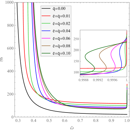
Figure 1: Dependence of the energy $\tilde{E}$ of the vortex-Q-ball system on the phase frequency $\tilde{\omega}$ for different values of gauge coupling constants. The curves correspond to parameters $\tilde{m}=1$, $\tilde{g}=1$, $\tilde{h}=0.2$, $\tilde{\lambda}=0.125$, $\tilde{v}=2$, $N=1$, and $K=0$

The mixed boundary value problem (15)–(18), and (20) depends on the eight parameters: $m$, $g$, $h$, $\lambda$, $v$, $e$, $q$, and $\omega$. Without loss of generality, the number of the parameters can be reduced, if we rescale the radial variable $r$ and the ansatz function $\sigma$ as follows:

$$r=m^{-1}\tilde{r},\;\sigma=mg^{-1/2}\tilde{\sigma}.$$ (100)

After rescaling, the vortex-Q-ball system will be described solely by the six dimensionless parameters: $\tilde{h}=m^{2}g^{-2}h$, $\tilde{\lambda}=gv^{4}m^{-4}\lambda$, $\tilde{v}=g^{1/2}m^{-1}v$, $\tilde{e}=g^{-1/2}e$, $\tilde{q}=g^{-1/2}q$, and $\tilde{\omega}=m^{-1}\omega$, whereas the two dimensionless parameters $\tilde{m}$ and $\tilde{g}$ will be equal to 1. In most numerical calculations, we use the following values for the nongauged dimensionless parameters: $\tilde{h}=0.2$, $\tilde{\lambda}=0.125$, $\tilde{v}=2$. The dimensionless gauge coupling constants $\tilde{e}$ and $\tilde{q}$ are taken to be equal ($\tau=\tilde{q}/\tilde{e}=1$), and may vary in some interval. In addition to these parameters, the mixed boundary value problem (15)–(18), and (20) also depends on the two integers: $N$ (topological winding number of the vortex component) and $K$ (nontopological winding number of the Q-ball component). We shall consider the vortex-Q-ball systems with the vortex winding number $N=1$, while the Q-ball winding number $K$ may take a range of values.

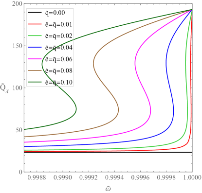
Figure 2: Dependence of the Noether charge $\tilde{Q}_{\chi}$ of the vortex-Q-ball system on the dimensionless phase frequency $\tilde{\omega}$ in the vicinity of $\tilde{\omega}=1$. The parameters of the vortex-Q-ball system are the same as in Fig. 1

Figure 1 shows the dependence of the dimensionless energy $\tilde{E}=gm^{-2}E$ of the vortex-Q-ball system on the dimensionless phase frequency $\tilde{\omega}=m^{-1}\omega$. The presented curves correspond to the vortex-Q-ball system at six different values of the gauge coupling constants and to the nongauged two-dimensional Q-ball. We see that with decreasing $\tilde{\omega}$, the system passes into the thin-wall regime in which the energy and the Noether charge increase indefinitely. When $\tilde{\omega}\rightarrow 1$, the vortex-Q-ball system passes into the thick-wall regime. In this regime, the behaviour of the vortex-Q-ball system differs considerably from that of the nongauged two-dimensional Q-ball. In particular, the energy of the Q-ball decreases monotonically as $\tilde{\omega}\rightarrow 1$, whereas the behaviour of the energy of the vortex-Q-ball system is more complicated, as follows from the subplot in Fig. 1. We see that for the vortex-Q-ball system, the curves $\tilde{E}(\tilde{\omega})$ are $s$-shaped in the vicinity of $\tilde{\omega}=1$. This fact is due to the nontrivial interaction between the vortex and Q-ball components of the soliton system. Note that in Ref. loginov_plb_777 , we have not managed to obtain, by numerical methods, the $s$-shaped parts of the $\tilde{E}(\tilde{\omega})$ and $\tilde{Q}_{\chi}(\tilde{\omega})$ curves.

It follows from the subplot in Fig. 1 that the limit value $\tilde{E}(1)$ is not a constant for the vortex-Q-ball system, but increases with a decrease of $\tilde{e}$. It was found numerically that for small values of $\tilde{e}$, the value $\tilde{E}(1)\approx a+b\ln(\tilde{e}^{-1})$, where $a$ and $b$ depend on the gauge coupling constants through the ratio $\tau=\tilde{q}/\tilde{e}$ in accordance with the conclusion of Sect. 4.

Beyond the neighbourhood of $\tilde{\omega}=1$, the rescaled Noether charge $\tilde{Q}_{\chi}=gm^{-1}Q_{\chi}$ depends on $\tilde{\omega}$ similar to the dimensionless energy $\tilde{E}=gm^{-2}E$ in Fig. 1. However, the behaviour of the curves $\tilde{Q}_{\chi}(\tilde{\omega})$ and $\tilde{E}(\tilde{\omega})$ is different in the neighbourhood of $\tilde{\omega}=1$. Indeed, Figs. 2 and 3 show the curves $\tilde{Q}_{\chi}(\tilde{\omega})$ in neighbourhoods of $\tilde{\omega}=1$ for different values of the gauge coupling constants. The curves in Fig. 2 correspond to the same values of the gauge coupling constant as in Fig. 1, while those in Fig. 3 correspond to larger values of the gauge coupling constants. We see that unlike the curves $\tilde{E}(\tilde{\omega})$ in the subplot in Fig. 1, the curves $\tilde{Q}_{\chi}(\tilde{\omega})$ end at the same point. It follows that the limiting thick-wall value $\tilde{Q}_{\chi}(1)$ does not depend on the gauge coupling constants $\tilde{e}$ and $\tilde{q}$ separately. Instead, it depends only on their ratio $\tau=\tilde{q}/\tilde{e}$ in accordance with the conclusion of Sect. 4.

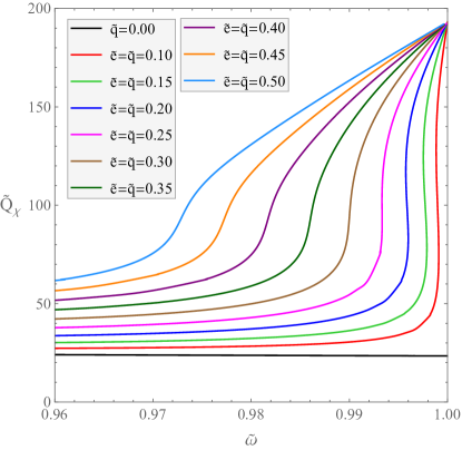
Figure 3: The same as in Fig. 2, but for large values of the gauge coupling constants

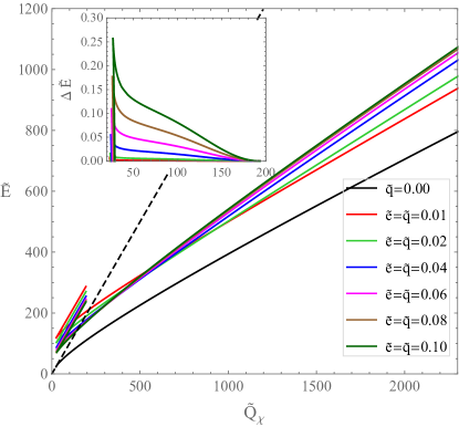
Figure 4: Dependence of the energy $\tilde{E}$ of the vortex-Q-ball system on the Noether charge $\tilde{Q}_{\chi}$ for different values of the gauge coupling constants. The straight dashed line corresponds to the linear dependence $\tilde{E}=\tilde{Q}_{\chi}$. The subplot presents the dependence of the difference $\Delta\tilde{E}=\tilde{E}-\tilde{Q}_{\chi}-\tilde{E}_{\text{v }}$ on $\tilde{Q}_{\chi}$ in the neighbourhood of cuspidal points

Figures 2 and 3 show that the form of the curves $\tilde{Q}_{\chi}(\tilde{\omega})$ changed with the increase in the gauge coupling constants. In Fig. 2, the curves $\tilde{Q}_{\chi}(\tilde{\omega})$ are $s$-shaped similar to the curves $\tilde{E}(\tilde{\omega})$ in the subplot in Fig. 1. At the same time, it follows from Fig. 3 that by increasing the gauge coupling constants, the curves $\tilde{Q}_{\chi}(\tilde{\omega})$ cease to be $s$-shaped, and the turning points of $s$-shaped $\tilde{Q}_{\chi}(\tilde{\omega})$ curves turn into a single inflection point of monotonically increasing $\tilde{Q}_{\chi}(\tilde{\omega})$ curves.

Figure 4 presents the energy $\tilde{E}$ of the vortex-Q-ball system as a function of its Noether charge $\tilde{Q}_{\chi}$ for the same values of the gauge coupling constants as in Fig. 1. We see that all the curves $\tilde{E}(\tilde{Q}_{\chi})$ that correspond to the vortex-Q-ball system have one cuspidal point, whereas there is no cuspidal point on the curve $\tilde{E}(\tilde{Q}_{\chi})$ for the two-dimensional nongauged Q-ball. The next characteristic feature is that the $\tilde{Q}_{\chi}$-coordinates for the rightmost points of the upper branches of the curves $\tilde{E}(\tilde{Q}_{\chi})$ coincide. Of course, this is a consequence of the fact that the value $\tilde{Q}_{\chi}(1)$ depends on $\tilde{e}$ and $\tilde{q}$ only through the ratio $\tau=\tilde{q}/\tilde{e}$, which is the same for all vortex-Q-ball curves in Fig. 4.

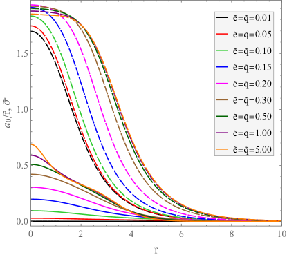
Figure 5: Profile functions $a_{0}/\tilde{r}$ (solid curves) and $\tilde{\sigma}$ (dashed curves) of the vortex-Q-ball system for different values of the gauge coupling constants. The curves correspond to parameters $\tilde{\omega}=0.7$, $\tilde{m}=1$, $\tilde{g}=1$, $\tilde{h}=0.2$, $\tilde{\lambda}=0.125$, $\tilde{v}=2$, $N=1$, and $K=0$

In Fig. 4, the dashed straight line corresponds to the plane-wave field configuration of the complex scalar field $\chi$. We see that the energy of the two-dimensional nongauged $Q$-ball is less than that of the plane-wave field configuration, except for the point of contact, at which they are equal. Hence, the two-dimensional nongauged $Q$-ball is stable against decay into massive scalar $\chi$-bosons. It follows from Fig. 4 that except for the neighbourhood of cuspidal points, the energy of the vortex-Q-ball system is less than that of the plane-wave field configuration. Hence, the Q-ball component of the vortex-Q-ball system is stable against decay into massive scalar $\chi$-bosons provided that $\tilde{E}<\tilde{Q}_{\chi}$.

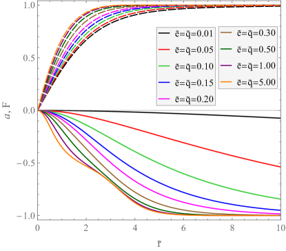
Figure 6: Profile functions $a$ (solid curves) and $F$ (dashed curves) of the vortex-Q-ball system for different values of the gauge coupling constants. The parameters of the vortex-Q-ball system are the same as in Fig. 5

To ascertain the possibility of decay of the Q-ball component of the vortex-Q-ball system, we introduce the value $\Delta\tilde{E}=\tilde{E}-\tilde{Q}_{\chi}-\tilde{E}_{\text{v}}$, where $\tilde{E}_{\text{v}}$ is the energy of the vortex component of the system. We define $\tilde{E}_{\text{v}}$ as the energy of the ANO vortex at a given value of the gauge coupling constant $\tilde{e}$. The curves $\tilde{E}_{\text{v}}(\tilde{Q}_{\chi})$ are presented in the subplot in Fig. 4. It is obvious that decay of the $Q$-ball component into scalar $\chi$-bosons is possible only if $\Delta\tilde{E}$ is positive. It follows from the subplot in Fig. 4 that for all gauge coupling constants, $\Delta\tilde{E}$ is positive on the upper branches of curves $\tilde{E}(\tilde{Q}_{\chi})$. Furthermore, $\Delta\tilde{E}$ is also positive on the lower branches of $\tilde{E}(\tilde{Q}_{\chi})$ curves in neighbourhoods of their cuspidal points. Hence, the vortex-Q-ball system is unstable in the area presented in the subplot in Fig. 4. The instability, however, can be either classical (the presence of one or more unstable modes in the functional neighbourhood of the soliton system) or quantum-mechanical (the possibility of quantum tunneling of the soliton system to another state). It was shown in Refs. lee_pang ; fried_lee that the appearance of a cusp on the energy-Noether charge curve indicates the onset of a mode of instability. Hence, the Q-ball components of the soliton systems lying on the upper branches of the $\tilde{E}(\tilde{Q}_{\chi})$ curves are classically unstable.

Next we present the ansatz functions of the vortex-Q-ball system for different values of gauge coupling constants. Figure 5 presents the ansatz functions $a_{0}(\tilde{r})/\tilde{r}$ and $\tilde{\sigma}(\tilde{r})$, and Figure 6 presents the ansatz functions $a(\tilde{r})$ and $F(\tilde{r})$. It follows from Fig. 5 that $\left.a_{0}\left(\tilde{r}\right)/\tilde{r}\right|_{\tilde{r}=0}$ increases monotonically and $a_{0}\left(\tilde{r}\right)/\tilde{r}$ tends to limiting form (70a) as $\tilde{e}$ and $\tilde{q}$ increase. In particular, $\left.a_{0}\left(\tilde{r}\right)/\tilde{r}\right|_{\tilde{r}=0}$ reaches the maximum limit value $\tilde{\omega}/\tau=0.7$ as $\tilde{e}=\tilde{q}\rightarrow\infty$, which is consistent with Eqs. (42) and (70a). The ansatz function $\tilde{\sigma}(\tilde{r})$ also tends to a limiting form as the gauge coupling constants increase indefinitely. Figure 6 shows that similar to $a_{0}(\tilde{r})/\tilde{r}$, the ansatz function $a(\tilde{r})$ is sensitive to the magnitude of $\tilde{e}$ and $\tilde{q}$. In particular, it tends to zero at any finite $\tilde{r}$ as $\tilde{e}=\tilde{q}\rightarrow 0$ and tends to limiting form (70b) as $\tilde{e}=\tilde{q}\rightarrow\infty$. The dependence of $F(\tilde{r})$ on the the gauge coupling constants is not as strong as that of $a(r)$. It follows from Fig. 6 that $F(\tilde{r})$ tends to a limiting form as $\tilde{e}=\tilde{q}\rightarrow\infty$ and to the global vortex solution as $\tilde{e}=\tilde{q}\rightarrow 0$.

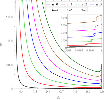
Figure 7: Dependence of the energy $\tilde{E}$ of the vortex-Q-ball system on the phase frequency $\tilde{\omega}$ for the first few radially excited states. The curves correspond to parameters $\tilde{m}=1$, $\tilde{g}=1$, $\tilde{h}=0.2$, $\tilde{\lambda}=0.125$, $\tilde{v}=2$, $\tilde{e}=\tilde{q}=0.1$, $N=1$, and $K=0$

Like two and three-dimensional nongauged Q-balls, radially excited states in the vortex-Q-ball system exist. In Fig. 7, we can see the curves $\tilde{E}(\tilde{\omega})$ for the unexcited ($n=0$) and the first six ($n=1,\ldots,6$) radially excited states of the vortex-Q-ball system. As in the previous (unexcited) case, the radially excited system passes into the thin-wall regime as $\tilde{\omega}\rightarrow\tilde{\omega}_{\text{tn}}$ and into the thick-wall regime as $\tilde{\omega}\rightarrow 1$. Like curves in Fig. 1, the curves $\tilde{E}(\tilde{\omega})$ of radially excited vortex-Q-ball systems are $s$-shaped in the vicinity of $\tilde{\omega}=1$. Next, we see that at fixed $\tilde{\omega}$, the energy of the the vortex-Q-ball system increases with an increase in $n$. It was found numerically that at fixed $\tilde{\omega}$, the energy and Noether charge increase quadratically in $n$ starting with $n=2$:

$$\tilde{E}\approx a+bn^{2},\;\tilde{Q}_{\chi}\approx c+dn^{2},$$ (101)

where $a$ and $b$ are positive constants, whereas the signs of constants $c$ and $d$ coincide with that of $\tilde{\omega}$. The behaviour of $\tilde{Q}_{\chi}(\tilde{\omega})$ curves is similar to that of $\tilde{E}(\tilde{\omega})$ curves in Fig. 7. In particular, the values $\tilde{Q}_{\chi}(1)$ are different for different $n$.

Figure 8 presents the curves $\tilde{E}(\tilde{Q}_{\chi})$ for the unexcited and the first six radially excited states of the vortex-Q-ball system. All curves $\tilde{E}(\tilde{Q}_{\chi})$ have cuspidal points in which $\tilde{E}$ and $\tilde{Q}_{\chi}$ reach minimum values. Numerically, we found that starting with $n=2$, the minimum values of $\tilde{Q}_{\chi}$ in the cusp points are well described by a quadratic dependence: $Q_{\chi\text{c}}=a_{\text{c}}+b_{\text{c}}n^{2}$. It follows that at a given $\tilde{Q}_{\chi}$, the number of radially excited states of the vortex-Q-ball system does not exceed

$$n_{\max}=\left\lfloor b_{\text{c}}^{-1/2}\left(\tilde{Q}_{\chi}-a_{\text{c}}\right)^{1/2}\right\rfloor,$$ (102)

where $\lfloor x\rfloor$ denotes the floor of $x$ (the greatest integer less than or equal to $x$). We see that at large $\tilde{Q}_{\chi}$, the number of radially excited states rises $\propto\tilde{Q}_{\chi}^{1/2}$.

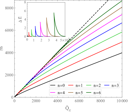
Figure 8: Dependence of the energy $\tilde{E}$ of the vortex-Q-ball system on the Noether charge $\tilde{Q}_{\chi}$ for the first few radially excited states. The straight dashed line corresponds to the linear dependence $\tilde{E}=\tilde{Q}_{\chi}$. The subplot presents the dependence of the difference $\Delta\tilde{E}=\tilde{E}-\tilde{Q}_{\chi}-\tilde{E}_{\text{v}}$ on $\tilde{Q}_{\chi}$ in neighbourhoods of cuspidal points

It follows from Fig. 8 that at a given $\tilde{Q}_{\chi}$, the lower-branch energy $\tilde{E}$ increases with $n$. Hence, radially excited vortex-Q-ball states lying on lower branches of $\tilde{E}(\tilde{Q}_{\chi})$ curves are unstable with respect to the transition into less excited states. Furthermore, we can see from the subplot in Fig. 8 that the Q-ball components of radially excited vortex-Q-ball states are unstable with respect to decay into scalar $\chi$-bosons in neighbourhoods of cuspidal points (the upper branches and small parts of the lower branches of $\tilde{E}(\tilde{Q}_{\chi})$ curves).

Figures 9 and 10 present ansatz functions for the first 10 radially excited states of the vortex-Q-ball system. We see from Fig. 9 that oscillations of the $\tilde{\sigma}(\tilde{r})$ curves are inharmonious. In particular, amplitudes of peaks and valleys of $\tilde{\sigma}(\tilde{r})$ curves are decreased with the increase in the number of oscillations, whereas the distances between adjacent peaks and valleys of $\tilde{\sigma}(\tilde{r})$ curves are increased. As seen in Fig. 10, the ansatz functions $\tilde{a}_{0}(\tilde{r})/\tilde{r}$ and $a(\tilde{r})$ also oscillate. In particular, the positions of local maxima of $\tilde{a}_{0}(\tilde{r})/\tilde{r}$ and $a(\tilde{r})$ approximately coincide with those of peaks and valleys of $\tilde{\sigma}(\tilde{r})$, whereas the positions of local minima of $\tilde{a}_{0}(\tilde{r})/\tilde{r}$ and $a(\tilde{r})$ are approximately the same as those of nodes (zeros) of $\tilde{\sigma}(\tilde{r})$.

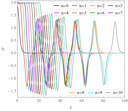
Figure 9: Profile functions $\tilde{\sigma}$ for the first 10 radially excited states of the vortex-Q-ball system. The curves correspond to parameters $\tilde{\omega}=0.7$, $\tilde{m}=1$, $\tilde{g}=1$, $\tilde{h}=0.2$, $\tilde{\lambda}=0.125$, $\tilde{v}=2$, $\tilde{e}=\tilde{q}=0.1$, $N=1$, and $K=0$

It was shown in Ref. loginov_prd_102 that the number of radially excited states of the three-dimensional gauged Q-ball is finite. At the same time, we found no indication of the finiteness of the number of radially excited states for the vortex-Q-ball system. Of course, the reason for this difference is that the three-dimensional gauged Q-ball possesses an electrical charge, whereas the two-dimensional vortex-Q-ball system is electrically neutral. As a result, the electric charge density of the three-dimensional gauged Q-ball is always either positive or negative, whereas that for the vortex-Q-ball system is alternating. This difference is apparent in the behaviour of the ansatz function $\Omega(r)$ defined in Eq. (40). Indeed, it is shown in Ref. klee that in the case of the three-dimensional gauged Q-ball, $\Omega(r)$ is a bounded ($0<\Omega(r)<\omega$) and monotonically increasing function of $r$. For the vortex-Q-ball system, the ansatz function $\Omega(r)$ is also bounded in the interval $(0,\omega)$ as it is seen from Eq. (41). However, $\Omega(r)$ need not be monotonic in this case. Indeed, the oscillating behaviour of $\tilde{a}_{0}(\tilde{r})/\tilde{r}$ shown in Fig. 10 results in the oscillating behaviour of $\Omega(\tilde{r})=\omega-\tau\tilde{a}_{0}(\tilde{r})/\tilde{r}$. The monotonic increase of $\Omega(r)$ leads to the restriction of the number of radially excited states for the three-dimensional gauged Q-ball, because in this case, $\Omega(r)$ reaches its maximum value $\omega$ for a finite number of oscillations of $\sigma(r)$. In contrast, the nonmonotonic oscillating behaviour of $\Omega(r)$ makes it possible for vortex-Q-ball systems with an arbitrarily large number of oscillations (and hence nodes) of $\sigma(r)$ to exist; thus, there are no restrictions on the number of radially excited states of the vortex-Q-ball system.

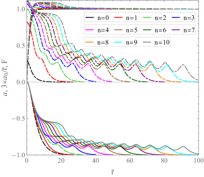
Figure 10: Ansatz functions $a$, $3a_{0}/\tilde{r}$, and $F$ for the first 10 radially excited states of the vortex-Q-ball system. The parameters of the vortex-Q-ball system are the same as in Fig. 9

Now we turn to a description of the vortex-Q-ball’s states with nonzero integer-valued parameter $K$. Figure 11 shows the curves $\tilde{E}(\tilde{\omega})$ for the first few states with nonzero $K$. It follows from Fig. 11 that any two $\tilde{E}(\tilde{\omega})$ curves whose parameters $K^{\prime}$ and $K^{\prime\prime}$ satisfy the condition $K^{\prime}+K^{\prime\prime}=2$ tend to the same limit in the thick-wall regime when $\tilde{\omega}\rightarrow 1$. A similar statement is valid for the $\tilde{Q}_{\chi}(\tilde{\omega})$ curves. This facts can be explained as follows. In the thick-wall regime, the limiting energy of the vortex-Q-ball system is written as $E_{\text{tk}}=F_{0}+2m^{2}\bar{F}_{2}$, where $F_{0}$ is the energy of the ANO vortex with a given $e$, and $2m^{2}\bar{F}_{2}$ is the energy of the Q-ball component. It follows from Eq. (81) that $\bar{F}_{2}$ is expressed solely in terms of the rescaled ansatz function $\bar{\sigma}$. Next, the rescaled ansatz function $\bar{\sigma}$ satisfies differential equation (86). We see that Eq. (86) depends on the integer-valued parameters $K$ and $N$ only through the combination $\varkappa=(K-\tau N)^{2}$. It follows that the parameters $K^{\prime}$ and $K^{\prime\prime}$, which satisfy the relation $K^{\prime}+K^{\prime\prime}=2\tau N$, lead to the same value of $\varkappa$. Because both $K^{\prime}$ and $K^{\prime\prime}$ are integers, the value of $2\tau N$ is also an integer, thus the parameter $\tau=e/q$ is an integer or half-integer. If $2\tau N$ is a noninteger, then $\tilde{E}(\tilde{\omega})$ curves corresponding to different $K$ will not tend to the same limit as $\tilde{\omega}\rightarrow 1$. In our case, the parameters $N$ and $\tau$ are equal to one, so $2\tau N=2$. Thus, differential equation (86) will have the same form for any two vortex-Q-ball systems whose parameters satisfy the condition $K^{\prime}+K^{\prime\prime}=2$.

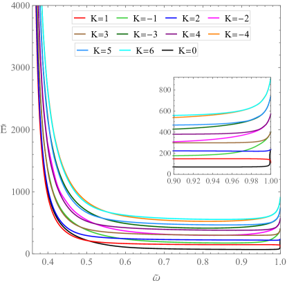
Figure 11: Dependence of the energy $\tilde{E}$ of the vortex-Q-ball system on the phase frequency $\tilde{\omega}$ for the first few azimuthally excited states. The curves correspond to parameters $\tilde{m}=1$, $\tilde{g}=1$, $\tilde{h}=0.2$, $\tilde{\lambda}=0.125$, $\tilde{v}=2$, $\tilde{e}=\tilde{q}=0.1$, and $N=1$

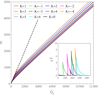
Figure 12: Dependence of the energy $\tilde{E}$ of the vortex-Q-ball system on the Noether charge $\tilde{Q}_{\chi}$ for the first few azimuthally excited states. The straight dashed line corresponds to the linear dependence $\tilde{E}=\tilde{Q}_{\chi}$. The subplot presents the dependence of the difference $\Delta\tilde{E}=\tilde{E}-\tilde{Q}_{\chi}-\tilde{E}_{\text{v}}$ on $\tilde{Q}_{\chi}$ in neighbourhoods of cuspidal points

Eq. (86) is valid for all $\bar{r}$ except those in the interval $0\leq\bar{r}\lesssim\Delta_{\omega}m_{A,\phi}^{-1}$ whose width tends to zero in the thick-wall regime. This is because the rescaled ansatz functions $\bar{a}(\bar{r})\equiv a(\Delta_{\omega}^{-1}\bar{r})$ and $\bar{F}(\bar{r})\equiv F(\Delta_{\omega}^{-1}\bar{r})$ are different from their limiting values in this infinitesimal interval of $\bar{r}$. Next, the ansatz functions $\bar{\sigma}_{K^{\prime}}(\bar{r})$ and $\bar{\sigma}_{K^{\prime\prime}}(\bar{r})$ (the dependence of $\bar{\sigma}$ on $K$ is shown explicitly) satisfy the same boundary conditions: $\bar{\sigma}(0)=0$ and $\bar{\sigma}(\infty)=0$. The only exception is in the case $K=0$ for which the left boundary condition is $\bar{\sigma}^{\prime}(0)=0$. However, it was found numerically that in this case, $\bar{\sigma}(0)\rightarrow 0$ as $\Delta_{\omega}\rightarrow 0$, and the left boundary condition for $K^{\prime}=0$ becomes essentially the same as that for the complementary case $K^{\prime\prime}=2$. It follows that the ansatz functions $\bar{\sigma}_{K^{\prime}}(\bar{r})$ and $\bar{\sigma}_{K^{\prime\prime}}(\bar{r})$ that satisfy the condition $K^{\prime}+K^{\prime\prime}=2$ tend to the same limit in the thick-wall regime and so do the corresponding functionals $\bar{F}_{2K^{\prime}}$ and $\bar{F}_{2K^{\prime\prime}}$. Hence, the energies (Noether charges) of the two vortex-Q-ball systems with $K^{\prime}+K^{\prime\prime}=2$ tend to the same value in the thick-wall regime. Note that there is no complementary vortex-Q-ball system for the system with $K=1$. Indeed, in this case the parameters $K^{\prime}$ and $K^{\prime\prime}$ are the same: $K^{\prime}=1,K^{\prime\prime}=1\Rightarrow K^{\prime}+K^{\prime\prime}=2$.

It follows from Eq. (47) that the two vortex-Q-ball systems with the same Noether charges and with integer parameters $K^{\prime}$ and $K^{\prime\prime}$ such that $K^{\prime}+K^{\prime\prime}=2\tau N$ possess the opposite angular momenta. Hence, the angular momenta of two vortex-Q-ball systems with $K^{\prime}+K^{\prime\prime}=2$ tend to the opposite values in the thick-wall regime, whereas the angular momentum of the state with $K=1$ vanishes.

Figure 12 presents the $\tilde{E}({\tilde{Q}_{\chi}})$ curves for the same $K$ as in Fig. 11. We see that just as in Figs. 4 and 8, the curves $\tilde{E}({\tilde{Q}_{\chi}})$ have cuspidal points. The only exception is the $\tilde{E}({\tilde{Q}_{\chi}})$ curve for $K=1$; in this case, the absence of a cuspidal point follows from the monotonicity of the corresponding $\tilde{E}({\tilde{\omega}})$ curve in Fig. 11. The conservation of the Noether charge and the angular momentum leads to the conclusion that the parts of $\tilde{E}({\tilde{Q}_{\chi}})$ curves lying below the line $\tilde{E}=\tilde{E}_{\text{v}}+\tilde{Q}_{\chi}$ correspond to stable vortex-Q-ball systems. In the subplot in Fig. 12, we can see the parts of $\tilde{E}({\tilde{Q}_{\chi}})$ curves that lie above the line $\tilde{E}=\tilde{E}_{\text{v}}+\tilde{Q}_{\chi}$ and thus correspond to unstable vortex-Q-ball systems.

It follows from Fig. 12 that the curves $\tilde{E}_{K^{{}^{\prime}}}(\tilde{Q_{\chi}})$ and $\tilde{E}_{K^{{}^{\prime\prime}}}(\tilde{Q_{\chi}})$ with $K^{\prime}+K^{\prime\prime}=2\tau N=2$ approximately coincide starting with $\left(K^{\prime},K^{\prime\prime}\right)=(4,-2)$. Hence, the energies of the two vortex-Q-ball systems that correspond to coincident curves $\tilde{E}_{K^{{}^{\prime}}}(\tilde{Q_{\chi}})$ and $\tilde{E}_{K^{{}^{\prime\prime}}}(\tilde{Q_{\chi}})$ are approximately the same at given $Q_{\chi}$. Note that the parameter $K-\tau N$ has opposite values for the curves $\tilde{E}_{K^{{}^{\prime}}}(\tilde{Q_{\chi}})$ and $\tilde{E}_{K^{{}^{\prime\prime}}}(\tilde{Q_{\chi}})$ with $K^{\prime}+K^{\prime\prime}=2\tau N$. Hence, the angular momenta $\tilde{J}_{K^{{}^{\prime}}}(\tilde{Q_{\chi}})$ and $\tilde{J}_{K^{{}^{\prime\prime}}}(\tilde{Q_{\chi}})$ are opposite as it follows from Eq. (47). It follows from Eqs. (49a)–(49c) that under the reverse $(K,N)\rightarrow(-K,-N)$, the angular momentum of the vortex-Q-ball system changes the sign, whereas the energy and the Noether charge remains the same. The parameter $K-\tau N$ also changes the sign under the reverse $(K,N)\rightarrow(-K,-N)$. Hence, the functions $E(N,K)$, $Q_{\chi}(N,K)$, and $J(N,K)$ in essence become functions of one argument $K-\tau N$ when the parameter $\left|K-\tau N\right|\gtrsim 3$.

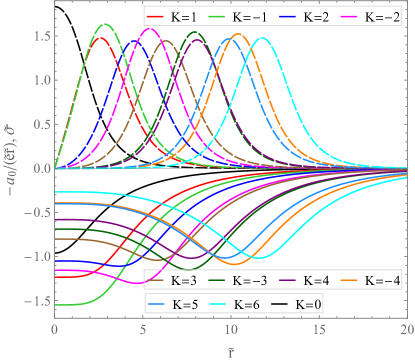
Figure 13: Profile functions -$a_{0}/(\tilde{e}\tilde{r})$ (solid curves) and $\tilde{\sigma}$ (dashed curves) of the vortex-Q-ball system for the first few azimutally excited states. The curves correspond to parameters $\tilde{\omega}=0.7$, $\tilde{m}=1$, $\tilde{g}=1$, $\tilde{h}=0.2$, $\tilde{\lambda}=0.125$, $\tilde{v}=2$, $\tilde{e}=\tilde{q}=0.1$, and $N=1$

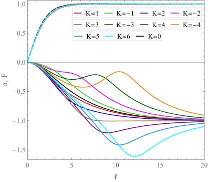
Figure 14: Ansatz functions $a$ (solid curves) and $F$ (dashed curves) of the vortex-Q-ball system for the first few azimuthally excited states. The parameters of the vortex-Q-ball system are the same as in Fig. 13

The reason for this is the presence of the centrifugal term $-r^{-2}\left(K+\tau a\left(r\right)\right)^{2}\sigma\left(r\right)$ in Eq. (18). The contribution of this term is proportional to $r^{-2}\left(K-\tau N\right)^{2}$ when $a(r)$ is in the vicinity of the limiting value of $-N$. The growth of $\left|K-\tau N\right|$ leads to the growth of the factor $\varkappa=\left(K-\tau N\right)^{2}$ in the centrifugal term. The growth of $\varkappa$ must be compensated, otherwise, the solution of mixed boundary value problem (15)–(18) and (20) will not exist. Such compensation is achieved through the shift of the ansatz function $\sigma(r)$ towards higher values of $r$. The shift results in reducing the factor $r^{-2}$ in the centrifugal term which compensates for the growth of the factor $\varkappa$. With increasing $r$, it is convenient to pass to the new ansatz function $\Delta a(r)=N+a(r)$. Then the system (15)–(18) will depend on the parameters $K$ and $N$ only through the combination $K-\tau N$.

Figures 13 and 14 show the ansatz functions for the same $K$ as in Fig. 11. We see that for $K\neq 0$, the ansatz functions $\tilde{\sigma}(\tilde{r})$ have a slightly asymmetric bell-shaped form. Numerically, we found that the radial positions of maxima of the $\tilde{\sigma}(\tilde{r})$ curves increase approximately linearly with $\left|K-\tau N\right|$. It follows from Fig. 13 that with an increase in $\left|K-\tau N\right|$, the ansatz functions $a_{0}(\tilde{r})/(\tilde{e}\tilde{r})$ also form maxima whose radial positions are approximately the same as those of the corresponding $\tilde{\sigma}(\tilde{r})$ curves. Next, we see from Fig. 14 that the forms of $a(\tilde{r})$ curves strongly depend on $K-\tau N$. In particular, with an increase in $\left|K-\tau N\right|$, the minimum of $a(\tilde{r})$ appears for positive $K$ and the maximum (together with the left adjacent minimum) of $a(\tilde{r})$ appears for negative $K$. The radial positions of these extremes of $a(\tilde{r})$ approximately coincide with those of the maxima of the corresponding $\tilde{\sigma}(\tilde{r})$. Such a difference in the behaviour of the $a(\tilde{r})$ curves with positive and negative $K$ is explained by the fact that the driving term $-2eq(K-\tau N)\sigma(r)^{2}$ in Eq. (16) has the opposite sign in these cases. Finally, it follows from Fig. 14 that the forms of the $F(\tilde{r})$ curves weakly depend on $K$.

6 Conclusion

In the present paper, we continued the study of the vortex-Q-ball systems started in Ref. loginov_plb_777 . We investigated properties of the unexcited vortex-Q-ball systems at different values of gauge coupling constants and properties of radially excited vortex-Q-ball systems. We also investigated properties of azimuthally excited vortex-Q-ball systems. The vortex-Q-ball system is composed of a vortex (topological soliton) and a Q-ball (nontopological soliton), thus it combines properties of both topological and nontopological solitons. In particular, the vortex-Q-ball possesses a quantized magnetic flux and satisfies basic relation (13) for nontopological solitons.

The electromagnetic interaction between the vortex and Q-ball components results in significant changes in their properties. Firstly, the vortex and Q-ball components of the vortex-Q-ball system acquire opposite electrical charges, so the system remains electrically neutral as a whole. At the same time, neither ANO vortex nor two-dimensional Q-ball possess electrical charge because in gauge models without the Chern-Simons term, any two-dimensional electrically charged object will have infinite energy. Secondly, the vortex-Q-ball system possesses nonzero angular momentum despite the fact that both the ANO vortex and the two-dimensional axially symmetric Q-ball have zero angular momenta. Thirdly, the interaction between the vortex and Q-ball components leads to substantial change in the $E(\omega)$ and $E(Q_{\chi})$ curves for the vortex-Q-ball system in comparison with that of the two-dimensional nongauged Q-ball. In particular, in the case of the vortex-Q-ball system, some of $E(\omega)$ curves are $s$-shaped in the vicinity of $\omega=m$ and the $E(Q_{\chi})$ curves have cuspidal points, whereas none of these features hold for the two-dimensional nongauged Q-ball.

There exist several extreme regimes for the vortex-Q-ball system. We investigated four of them: the thick-wall regime in which the phase frequency $\omega$ tends to the maximum value, the thin-wall regime in which $\omega$ tends to the minimum value, and regimes of small and large gauge coupling constants. In particular, we found that the limiting thick-wall value of the Noether charge depends on the gauge coupling constants $e$ and $q$ only through the ratio $\tau=q/e$. We also found that the limiting thick-wall energies of two vortex-Q-ball systems whose azimuthal parameters $K^{\prime}$ and $K^{\prime\prime}$ satisfy the condition $K^{\prime}+K^{\prime\prime}=2\tau N$ are the same. As for extreme values of gauge coupling constants, the gauge field $A_{\mu}$ is decoupled from the vortex and Q-ball components as $q=\tau e\rightarrow 0$ and is expressed in terms of the scalar fields $\phi$ and $\chi$ as $q=\tau e\rightarrow\infty$. The latter means that the gauge field $A_{\mu}$ ceases to be a dynamic object as $q=\tau e\rightarrow\infty$.

Note that the very possibility of the existence of radially excited vortex-Q-ball states results from the nonlinear character of mixed boundary value problem (15)–(18) and (20). Indeed, a linear homogeneous boundary value problem is the Sturm–Liouville problem. Solutions with different numbers of nodes correspond to different eigenvalues of the Sturm–Liouville problem. It follows that these solutions satisfy different differential equations because the eigenvalue is a parameter of differential equation. In contrast, a nonlinear boundary value problem with fixed parameters may have more than one solution, as it is in the case of the vortex-Q-ball system. In this case, the second and subsequent solutions of the mixed nonlinear boundary value problem correspond to the radially excited states of the vortex-Q-ball system.

- (1) B. Julia, A. Zee, Phys. Rev. D 11, 2227 (1975). https://doi.org/10.1103/PhysRevD.11.2227
- (2) G. Rosen, J. Math. Phys. (N.Y.) 9, 999 (1968). https://doi.org/10.1063/1.1664694
- (3) K. Lee, J.A. Stein-Schabes, R. Watkins, L.M. Widrow, Phys. Rev. D 39, 1665 (1989). https://doi.org/10.1103/PhysRevD.39.1665
- (4) K.N. Anagnostopoulos, M. Axenides, E.G. Floratos, N. Tetradis, Phys. Rev. D 64, 125006 (2001). https://doi.org/10.1103/PhysRevD.64.125006
- (5) H. Arodz, J. Lis, Phys. Rev. D 79, 045002 (2009). https://doi.org/10.1103/PhysRevD.79.045002
- (6) T. Tamaki, N. Sakai, Phys. Rev. D 90, 085022 (2014). https://doi.org/10.1103/PhysRevD.90.085022
- (7) I.E. Gulamov, E.Ya. Nugaev, M.N. Smolyakov, Phys. Rev. D 89, 085006 (2014). https://doi.org/10.1103/PhysRevD.89.085006
- (8) J. Hong, Y. Kim, P.Y. Pac, Phys. Rev. Lett. 64, 2230 (1990). https://doi.org/10.1103/PhysRevLett.64.2230
- (9) R. Jackiw, E.J. Weinberg, Phys. Rev. Lett. 64, 2234 (1990). https://doi.org/10.1103/PhysRevLett.64.2234
- (10) R. Jackiw, K. Lee, E.J. Weinberg, Phys. Rev. D 42, 3488 (1990). https://doi.org/10.1103/PhysRevD.42.3488
- (11) D. Bazeia, G. Lozano, Phys. Rev. D 44, 3348 (1991). https://doi.org/10.1103/PhysRevD.44.3348
- (12) P.K. Ghosh, S.K. Ghosh, Phys. Lett. B 366, 199 (1996). https://doi.org/10.1016/0370-2693(95)01365-2
- (13) S.K. Paul, A. Khare, Phys. Lett. B 174, 420 (1986) https://doi.org/10.1016/0370-2693(86)91028-2
- (14) A. Khare, S. Rao, Phys. Lett. B 227, 424 (1989) https://doi.org/10.1016/0370-2693(89)90954-4
- (15) A. Khare, Phys. Lett. B 255, 393 (1991) https://doi.org/10.1016/0370-2693(91)90784-N
- (16) A.Yu. Loginov, V.V. Gauzshtein, Phys. Lett. B 784, 112 (2018). https://doi.org/10.1016/j.physletb.2018.07.044
- (17) C. dos Santos, E. da Hora, Eur. Phys. J. C 70, 1145 (2010). https://doi.org/10.1140/epjc/s10052-010-1490-4
- (18) L. Losano, J.M.C. Malbouisson, D. Rubiera-Garcia, C. dos Santos, EPL 101, 31001 (2013). https://doi.org/10.1209/0295-5075/101/31001
- (19) A.Yu. Loginov, Phys. Lett. B 777, 340 (2018). https://doi.org/10.1016/j.physletb.2017.12.054
- (20) A.Yu. Loginov, V.V. Gauzshtein, Eur. Phys. J. C 79, 780 (2019). https://doi.org/10.1140/epjc/s10052-019-7302-6
- (21) R. Friedberg, T.D. Lee, A. Sirlin, Phys. Rev. D 13, 2739 (1976). https://doi.org/10.1103/PhysRevD.13.2739
- (22) M.S. Volkov, E. Wöhnert, Phys. Rev. D 66, 085003 (2002). https://doi.org/10.1103/PhysRevD.66.085003
- (23) B. Kleihaus, J. Kunz, M. List, Phys. Rev. D 72, 064002 (2005). https://doi.org/10.1103/PhysRevD.72.064002
- (24) M. Mai, P. Schweitzer, Phys. Rev. D 86, 096002 (2012). https://doi.org/10.1103/PhysRevD.86.096002
- (25) A.Yu. Loginov, V.V. Gauzshtein, Phys. Rev. D 102, 025010 (2020). https://doi.org/10.1103/PhysRevD.102.025010
- (26) A.A. Abrikosov, Sov. Phys. JETP 5, 1174 (1957)
- (27) H.B. Nielsen, P. Olesen, Nucl. Phys. B 61, 45 (1973). https://doi.org/10.1016/0550-3213(73)90350-7
- (28) R. Friedberg, T.D. Lee, A. Sirlin, Nucl. Phys. B 115, 1 (1976). https://doi.org/10.1016/0550-3213(76)90274-1
- (29) R. Friedberg, T.D. Lee, A. Sirlin, Nucl. Phys. B 115, 32 (1976). https://doi.org/10.1016/0550-3213(76)90275-3
- (30) M. von Laue, Ann. Phys. (Leipzig) 340, 524 (1911). https://doi.org/10.1002/andp.19113400808
- (31) I. Bialynicki-Birula, Phys. Lett. A 182, 346 (1993). https://doi.org/10.1016/0375-9601(93)90406-P
- (32) J. Neu, Physica D 43, 385 (1990). https://doi.org/10.1016/0167-2789(90)90143-D
- (33) G.H. Derrick, J. Math. Phys. (N.Y.) 5, 1252 (1964). https://doi.org/10.1063/1.1704233
- (34) T.D. Lee, Y. Pang, Phys. Rep. 221, 251 (1992). https://doi.org/10.1016/0370-1573(92)90064-7
- (35) F. Paccetti Correia, M.G. Schmidt, Eur. Phys. J. C 21, 181 (2001). http://doi.org/10.1007/s100520100710
- (36) Maple User Manual, (Maplesoft, Waterloo, Canada, 2019), https://www.maplesoft.com
- (37) R. Friedberg, T.D. Lee, Phys. Rev. D 15, 1694 (1977). https://doi.org/10.1103/PhysRevD.15.1694