Rank/Select Queries over Mutable Bitmaps

Abstract.

The problem of answering rank/select queries over a bitmap is of utmost importance for many succinct data structures. When the bitmap does not change, many solutions exist in the theoretical and practical side. In this work we consider the case where one is allowed to modify the bitmap via a $\mbox{{flip}}(i)$ operation that toggles its $i$-th bit. By adapting and properly extending some results concerning prefix-sum data structures, we present a practical solution to the problem, tailored for modern CPU instruction sets. Compared to the state-of-the-art, our solution improves runtime with no space degradation. Moreover, it does not incur in a significant runtime penalty when compared to the fastest immutable indexes, while providing even lower space overhead.

1. Introduction

Given a bitmap $\mathcal{B}$ of $u$ bits where $n$ are set, the query $\mbox{{rank}}(i)$ asks for the number of bits set in $\mathcal{B}[0..i]$, for an index $0\leq i<u$; the query $\mbox{{select}}(i)$ asks for the position of the $i$-th bit set, for $0\leq i<n$ (in our formulation and throughout the paper, all indexes start from 0 so that if $\mbox{{select}}(i)=k$, then $\mbox{{rank}}(k)=i+1$). These queries are at the core of more complicated succinct data structures (Jacobson, 1988), whose objective is to support efficient operations on theoretically-optimal compressed data, i.e., within lower order terms from the theoretic minimum space. Important applications of succinct data structures include string dictionaries (Martínez-Prieto et al., 2016; Kanda et al., 2017), orthogonal range querying (Brisaboa et al., 2013) and filtering (Zhang et al., 2018), Web graphs representation (Brisaboa et al., 2014), text indexes (Ferragina et al., 2009), inverted indexes (Pibiri and Venturini, 2020b), just to name a few. For this reason, many solutions were proposed in both theory and practice to answer these queries efficiently with small extra space. It is intuitive that a data structure built on top of $\mathcal{B}$ – hereafter, named the index – helps in answering both queries faster, thus indicating that many space/time trade-offs are possible.

On the theoretical side, each of the two queries can be answered in $O(1)$ time with a separate index that just takes $o(u)$ extra bits (Clark, 1996; Jacobson, 1988). When both queries are to be supported using the same $o(u)$-bit index instead, it is not possible to do better than $O(\log u/\log w)$, where $w$ is the machine word size in bits (Fredman and Saks, 1989). The $o(u)$ term in space occupancy is also almost optimal (Miltersen, 2005; Golynski, 2007). Despite their elegance, these results are of little usefulness in practice because their corresponding indexes are either too complicated (i.e., with high constant factors and unpredictable memory accesses that impair efficiency) or take much space. Instead, practical solutions have now reached a mature state-of-the-art: depending on the size of the bitmap and the design of the index, both queries can be answered in (roughly speaking) tens of nanoseconds with $3-28\%$ of extra space.

Known solutions assume that the bitmap $\mathcal{B}$ is immutable. In this work we consider an extension to the problem defined above, where one is allowed to modify $\mathcal{B}$ with a $\mbox{{flip}}(i)$ operation that toggles $\mathcal{B}[i]$, the $i$-th bit of $\mathcal{B}$: the bit is set to 1 if it was 0 and vice versa, i.e., $\mathcal{B}[i]=\textsf{XOR}(\mathcal{B}[i],\mbox{{1}})$. We call this problem: rank/select queries over mutable bitmaps. We leave the bitmap uncompressed and we do not take into account compressed representations.

For example, suppose $\mathcal{B}$ is [01101101010101110], with $u=17$ and $n=10$. Then, $\mbox{{rank}}(7)=5$ and $\mbox{{select}}(7)=13$. If we perform $\mbox{{flip}}(3)$ and $\mbox{{flip}}(6)$, then $\mathcal{B}$ becomes [01111111010101110], so that now $\mbox{{rank}}(7)=7$ and $\mbox{{select}}(7)=9$.

Clearly, the index data structure should reflect the changes made on $\mathcal{B}$ and this complicates the problem compared to the immutable setting. We cannot hope of doing better than, again, $O(\log u/\log w)$ time for this problem, due to a lower bound by Fredman and Saks (1989). However, it is not clear what can be achieved in practice, which is our concern with this work. The problem is relevant for succinct dynamic data structures (Prezza, 2017), and other applications such as counting transpositions in an array and generating graphs by preferential attachment (Marchini and Vigna, 2020).

Our Contribution. Our solution to the problem builds on two main ingredients: (1) a space-efficient bitmap index that leverages SIMD instructions (Corporation, 2020) and other optimizations for fast query evaluation, and (2) efficient algorithms to solve the problem of rank/select over small, immutable, bitmaps. Regarding point (1), we adapt and extend a recent result (Pibiri and Venturini, 2020a) about the $b$-ary Segment-Tree, and show that SIMD is very effective to search and update the data structure. We describe two variants of the data structure, tailored for both the widespread AVX2 instruction set and the new AVX-512 one. As per point (2), we review, extend, and compare all existing approaches to perform rank/select over small bitmaps (e.g., 256 and 512 bits). These approaches include broadword techniques, intrinsics, SIMD instructions, or a combination of them. The results of the comparison may be of independent interest and relevant to other problems.

The best results for the two previous points are then combined to tune a mutable bitmap data structure with support for rank/select queries, with the aim of establishing new reference trade-offs. Compared to the state-of-the-art (Marchini and Vigna, 2020) (available as part of the Sux library (Vigna, 2020)), our solution is faster and consumes a negligible amount of extra space. We also compare the data structure against several other solutions for the immutable setting, implemented in popular libraries such as Sdsl (Gog et al., 2014; Gog and Petri, 2014), Succinct (Grossi and Ottaviano, 2013), and Poppy (Zhou et al., 2013). Our data structure is competitive with the fastest indexes and takes less space, while allowing clients to alter the bitmap as needed.

We publicly release the C++ implementation of the solutions proposed in this article at https://github.com/jermp/mutable_rank_select.

2. Related Work

In this section we review solutions devised to solve the problem of ranking and selection over mutable and immutable bitmaps.

2.1. Mutable Bitmaps

To the best of our knowledge, only Marchini and Vigna (2020) addressed the problem of rank/select over mutable bitmaps, providing a solution that uses a (compressed) Fenwick tree (Fenwick, 1994) as index. Therefore, this will be our direct competitor for this work. (To be fair, also the Dynamic library by Prezza (2017) contains a solution based on a B-tree but it is several times slower than the solution by Marchini and Vigna (2020), so we excluded it from our experimental analysis.)

Table 1. Summary of data structures. A space overhead indicated with $x-y\%$ is achieved by varying the density of the bitmap from 0.1 to 0.9.

Method	Index Design	Space Overhead	Reference
Rank9	2-level	25%	(Vigna, 2008, Sect. 3)
Rank9.v2	2-level	6.3%	(Gog and Petri, 2014, Sect. 3)
IL	1-level	12.5%	(Gog and Petri, 2014, Sect. 3)
Poppy	3-level	3%	(Zhou et al., 2013, Sect. 3.1)

(a) rank

Method	Index Design	Space Overhead	Reference
Rank9+Hinted	3-level	28%	(Grossi and Ottaviano, 2013, Sect. 3.3)
Clark’s	3-level	60%	(Clark, 1996)
MCL	2-level	$3-20\%$	(Gog and Petri, 2014, Sect. 4)
DArray	2-level	$6-51\%$	(Okanohara and Sadakane, 2007)
CS-Poppy	4-level	3.4%	(Zhou et al., 2013, Sect 3.2)

(b) select

2.2. Immutable Bitmaps

Solutions devised for the problem in the immutable setting abound in the literature. We summarize the main different approached in Table 1b.

Rank. The first data structure for constant-time rank was introduced by Jacobson (1988), and consists of a two-level index taking $O(u\log\log u/\log u)=o(u)$ bits of extra space. The index stores precomputed rank values for blocks of the bitmap, so that a query is resolved by accessing a proper value in each of the two levels. Vigna (2008) provided a seminal implementation of this data structure for blocks of 512 bits – known as Rank9 – by interleaving the data of the two levels to improve locality of reference. The data structure consumes 25% extra space. Gog and Petri (2014) presented two variants of Rank9: one consumes less space by resorting on larger block sizes; ($\approx$6% extra space); the other is more cache-friendly and interleaves the index with the bitmap itself. We refer to the former as Rank9.v2 and to the latter as IL.

Zhou et al. (2013) developed Poppy, a similar data structure to the space-efficient variant of Rank9 by Gog and Petri (2014). The main difference is that Poppy uses an additional level for the index, therefore allowing to design the two-level index using 32-bit integers, instead of 64-bit values. The extra space of Poppy is just 3%.

Select. The solutions developed for select can be broadly classified into two categories: rank-based and position-based. A rank-based solution answers queries by binary-searching an index developed for rank queries. The advantage is that the same index can be reused for both queries, so that select can be performed with no (or small) additional space to that of rank. Instead, position-based solutions are able to only answer select queries, thus, these take significant more space than rank-based approaches.

Vigna (2008) accelerated the binary search in the Rank9 index with an additional level that can quickly find the area to be searched, hence performing a hinted binary search. The original implementation requires 12% space overhead in addition to that of Rank9, that is, a total space overhead of 37%. Grossi and Ottaviano (2013) also implemented the hinted binary search with only 3% extra space, thus, the total space overhead becomes 28%.

A position-based solution builds an index storing sampled select results. The first data structure for constant-time queries was introduced by Clark (1996) and consists of a three-level index taking $3u/\lceil{\log\log u}\rceil+O(\sqrt{u}\log u\log\log u)$ bits of space in addition to the bitmap. However, a straightforward implementation consumes a lot of space, i.e., 60% (González et al., 2005). Gog and Petri (2014) simplified the implementation to reduce the space overhead (which can be up to 20%), and called it MCL. Okanohara and Sadakane (2007) proposed the DArray data structure, that essentially is Clark’s solution with 2 levels instead of 3.

Vigna (2008) proposed two data structures called Select9 and Simple. The Select9 data structure adds selection capabilities on top of Rank9. The space overhead depends on the density of the bits set in the bitmap (e.g., $25-32\%$ as reported by Vigna in his experimentation). Although the space overhead is larger than 25%, Select9 answers both queries. Instead, Simple does not depend on Rank9 and builds a two-level index following a similar idea to that of the DArray. The space overhead also depends on the density (e.g., $9-46\%$).

Zhou et al. (2013) proposed CS-Poppy that adds selection capabilities on top of Poppy, using the idea of combined sampling (Navarro and Providel, 2012). Since the additional index requires only 0.4% of extra space, the space overhead of Poppy is still very low, while also supporting select queries.

Compressed Layouts. Although in this work we do not aim at compressing the bitmap $\mathcal{B}$ nor its index, it is important to remark that a separate line of research studied the problem of Rank/Select queries over compressed bitmaps.

Okanohara and Sadakane (2007) proposed the first practical data structure that approaches $uH_{0}(\mathcal{B})+o(u)$ bits of space, where $H_{0}(\mathcal{B})\leq 1$ is the zero-th order empirical entropy of $\mathcal{B}$. However, the $o(u)$ term can be very large, except for very sparse bitmaps with densities below 5%. Navarro and Providel (2012) proposed a practical implementation of the compression scheme by Raman et al. (2007). The data structure has a space overhead of around 10% of $u$, on top of the entropy-compressed bitmap.

Of particular intrest for this work are the compressed solutions proposed by Grabowski and Raniszewski (2018), whose main concern is fast query support. We briefly sketch their data structures. In general, the bitmap is divided into blocks, and blocks are grouped into superblocks. For each block, a fixed-size header stores rank or select results. Depending on how headers and blocks are compressed, different layouts are derived and named: basic (no compression); basic with compressed header or bch (headers written differentially with respect to the first one); mono-pair elimination or mpe (a “mono-pair” is a block of $\mathcal{B}$ consisting in all 1s or 0s, thus not stored); cache-friendly or cf (results and offsets interleaved in a contiguous memory area). When the indexes are built for select, two parameters are used: a sampling value $\ell$ so that the result of $\mbox{{select}}(i\ell)$ is stored directly and a threshold value $T$ which determines the sparseness of the blocks. A block is considered to be sparse when $\mbox{{select}}((i+1)\ell)-\mbox{{select}}(i\ell)>T$, or dense otherwise. For a sparse block, all the results of $\mbox{{select}}(j)$ for $i\ell<j<(i+1)\ell$ are stored directly; for a dense block, the range of bits $\mathcal{B}[\mbox{{select}}(i\ell)+1..\mbox{{select}}((i+1)\ell)-1]$ is stored.

Experiments using real-world datasets show that the query time of their compressed layouts is competitive with that of the uncompressed counterparts.

3. Experimental Setup

Throughout the paper we discuss experimental results, so in this section we report the details of our setup and methodology. All the experiments were run on a single core of an Intel i9-9940X processor, clocked at 3.30 GHz. The processor has two private levels of cache memory per core: $2\times 32$ KiB $L_{1}$ cache (32 KiB for instructions and 32 KiB for data); 1 MiB for $L_{2}$ cache. The third level of cache, $L_{3}$, is shared among all cores and spans $\approx$19 MiB. All cache lines are 64-byte long. The processor has proper support for SSE, AVX, AVX2, and AVX-512, instruction sets.

Runtimes are reported in nanoseconds, measured by averaging among $1,000,000$ random queries. (In the plots, the minimum and maximum runtimes draw a “pipe”, with the marked line inside representing the average time.) Prior to measurement, an untimed run of queries is executed to warm-up the cache of the processor.

The whole codebase used for the experiments is written in C++ and available at https://github.com/jermp/mutable_rank_select. The code was tested under different UNIX platforms and compilers. For the experiments reported in the paper, the code was compiled with gcc 9.2.1 under Ubuntu 19.10 (Linux kernel 5.3.0, 64 bits), using the flags -std=c++17 -O3 -march=native.

4. Overview

⬇

template <typename SearchablePrefixSums, typename BlockType>

struct mutable_bitmap {

static const uint64_t block_size = BlockType::block_size;

static const uint64_t words_in_block = block_size / 64;

void build(uint64_t const* in, uint64_t num_64bit_words) {

uint64_t num_blocks = ceil(static_cast< double>(num_64bit_words) / words_in_block);

vector<uint16_t> counts;

counts.reserve(num_blocks);

bits.resize(words_in_block * num_blocks, 0);

memcpy(bits.data(), in, num_64bit_words * sizeof(uint64_t));

for (uint64_t i = 0; i != bits.size(); i += words_in_block) {

uint16_t val = 0;

for (uint64_t j = 0; j != words_in_block; ++j) {

val += __builtin_popcountll(bits[i + j]); // number of bits set in bits[i + j]

}

counts.push_back(val);

}

index.build(counts.data(), counts.size());

}

inline bool access(uint64_t i) const; // returns the i-th bit

void flip(uint64_t i) {

bool bit = access(i);

uint64_t word = i / 64, offset = i % 64, block = i / block_size;

bits[word] ^= 1ULL << offset;

index.update(block, bit);

}

uint64_t rank(uint64_t i) const {

uint64_t block = i / block_size, offset = i % block_size;

return (block ? index.sum(block - 1) : 0) +

BlockType::rank(&bits[words_in_block * block], offset);

}

uint64_t select(uint64_t i) const {

auto [block, sum] = index.search(i);

uint64_t offset = i - sum; // i - index.sum(block - 1);

return block_size * block + BlockType::select(&bits[words_in_block * block], offset);

}

private:

SearchablePrefixSums index;

vector<uint64_t> bits;

};

Figure 1. The C++ implementation of a mutable bitmap with flip/rank/select capabilities.

An elegant way to solve the problem of Rank/Select over a mutable bitmap is to divide the bitmap into blocks and use, as index, a searchable prefix-sum data structure that maintains the number of bits set into each block. It follows that operations rank/select can be implemented by first reading/searching the counters of the index and, then, concluding the query locally inside a block. The flip operation is instead supported by “adjusting” some counters of the index and toggling a bit of the bitmap. Therefore, the problem actually reduces to two distinct sub-problems:

1. The searchable prefix-sum problem, defined as follows. Given an array $A$ of $m$ integers, we are asked to support the following operations on $A$: $\mbox{{sum}}(i)$ returns the quantity $\sum_{k=0}^{i}A[k]$, $\mbox{{update}}(i,\Delta)$ sets $A[i]$ to $A[i]+\Delta$, and $\mbox{{search}}(x)$ returns the smallest $0\leq i<m$ such that $\mbox{{sum}}(i)>x$. (As explained shortly, we are only interested in the special case where $\Delta\in\{-1,+1\}$.)

2. Rank/Select over “small” bitmaps (i.e., the blocks) without auxiliary space.

We address these sub-problems in Section 5 and 6 respectively. The best results for these sub-problems are then combined to tune the final result in Section 7.

The example code in Figure 1 – the mutable_bitmap class – illustrates how a solution to the two aforementioned sub-problems can be exploited to solve the problem we are considering. In fact, note that rank uses the query index.sum(); select uses the query index.search(); and flip uses the operation index.update() with values of $\Delta$ restricted to be either $+1/-1$ (one more/less bit set inside a block).

Block Size. Before proceeding further, an important design decision has to be discussed – how to choose the block size. (Throughout the paper, we will refer to this quantity as $B$.) The block size determines space/time trade-offs: handling many small blocks can excessively enlarge the space (and query time) of the prefix-sum data structure; on the other hand, blocks that are too large take more time to be processed with a consequent query slowdown. For recent processors, the minimum block size should always be 64 bits given that both rank and select can be answered with a constant number of instructions over 64 bits (we provide further details about this in Section 6). For a reasonable space/time trade-off, the block size should be a small multiple of the word size, e.g., 256 or 512. For example, using blocks of 256 bits we expect a reduction in space overhead of (roughly) $256/64=4\times$ compared to the case of 64-bit blocks. For the rest of the paper, we will experiment with two block sizes – 256 and 512 bits. What makes these two sizes particularly appealing for modern processors is that (1) as long as no more than 512 bits are requested to be loaded, at most 1 cache-miss is generated because 512 bits is the (typical) cache-line size, and (2) we can process 256 and 512 bits of memory in parallel using the SIMD AVX2 and AVX-512 instruction sets.

Lastly, as we will better see in the following, this choice of block size plays an important role for the efficiency of the searchable prefix-sum data structure because some of its counters are sufficiently small as to permit packing several of these in a SIMD register for parallel processing.

5. The Searchable Prefix-Sum Data Structure

In this section we adapt and extend the $b$-ary Segment-Tree data structure with parallel updates proposed by Pibiri and Venturini to solve the prefix-sum problem (Pibiri and Venturini, 2020a). They determined that this data structure performs better than a binary Segment-Tree (Bentley, 1977; Bentley and Wood, 1980) and solutions based on the Fenwick-Tree (Fenwick, 1994). Before presenting our data structure, we recall some preliminary notions.

Given an array $A$ of $m$ integers, an internal node of a binary Segment-Tree stores the sum of the elements in $A[i,j]$, its left child that of $A[i,\lfloor(i+j)/2\rfloor]$, and its right child that of $A[\lfloor(i+j)/2\rfloor+1,j]$. The $i$-th leaf of the tree (from left to right) just stores $A[i]$ and the root the sum of the elements in $A[0,m-1]$. It is easy to generalize the tree to become $b$-ary: a node holds $b$ integers, the $i$-th being the sum of the elements of $A$ covered by the sub-tree rooted in its $i$-th child. Different trade-offs between the runtime of sum and update can be obtained by changing the solution adopted to solve such operations over the $b$ keys stored in a node.

Here is, in short, the solution by Pibiri and Venturini (2020a) assuming $A$ to be an array of (possibly signed) 64-bit integers. Every node of the tree is a two-level data structure, holding an array of $b$ keys, say $\mbox{{keys}}[0..b)$. This array is divided into segments of $\sqrt{b}$ keys each, and each segment stored in prefix-sum. A $\mbox{{summary}}[0..\sqrt{b})$ array stores the sums of the elements in each segment, again in prefix-sum. (Precisely, the $i$-th entry of summary is responsible for the segment $i-1$, and $\mbox{{summary}}[0]=0$.) It follows that sum queries are answered in constant time with $\mbox{{sum}}(i)=\mbox{{summary}}[i/\sqrt{b}]+\mbox{{keys}}[i]$; update operations are resolved by updating the summary array and the specific segment comprising the $i$-th key. Importantly, updates can be performed in parallel exploiting the fact that four 64-bit keys can be packed in a SIMD register of 256 bits.

Figure 2 shows an example of this organization for an input array of size $b=16$ containing only positive quantities as it is the case for the problem we are interested in this work.

Once a node of the tree has been modeled in this way, sum and update are resolved by traversing the tree by issuing the corresponding operation on one node per each level. Using reasonably large node fanouts $b$, the resulting tree is very flat, e.g., of height $\lceil\log_{256}m\rceil$, where $m$ is the array size and $b=256$. Taking this into account, Pibiri and Venturini (2020a) also recommend to write a specialized code path handling each possible value of tree height, which avoids the use of loops and branches during tree traversals for increased performance. In what follows, we adopt their two-level node layout and optimizations.

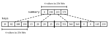
Figure 2. A two-level node layout built from array $[$19, 63, 106, 2, 13, 7, 0, 3, 151, 200, 9, 0, 0, 0, 143, 76$]$.

However, for the problem of rank/select over mutable bitmaps, we need to solve a specialized version of the prefix-sum problem, for the following reasons.

1. The input is an array of unsigned integers, with each value being at most 256 or 512 for our choice of block size.

2. The $\Delta$ value for update can only possibly be $+1$ or $-1$.

3. We also need the search operation, which we will implement using SIMD instructions.

Given these specifications, we first describe our Segment-Tree data structure tailored for AVX2 and, then, discuss how to extend it to the new AVX-512 instruction set. As explained before, we just need to care about the design of the tree nodes since every tree operation is a sequence of operations performed on the nodes.

5.1. Using AVX2

We start by highlighting some facts that will guide and motivate our design choices.

As per point (1) above, it follows that the integers stored in the tree are all unsigned. This fact poses a challenge on the applicability of SIMD instructions for updates and searches because most of such instructions (up to and including the AVX2 set) do not work with unsigned arithmetic. For example, it is not possible to compare unsigned integers natively but only signed quantities. Therefore, care should be put in ensuring that the sign bit remains always 0 to guarantee correctness of the algorithms which, in other words, limits the dynamic of the integers that can be loaded into a SIMD register. For example, we cannot ever store a quantity $v$ grater than $2^{15}-1$ in a 16-bit integer, otherwise the result of the comparison $v>x$ will be wrong for any $0\leq x<2^{15}$.

To make the overall tree height as small as possible, we would like to maximize the number of integers that we can pack in a 256-bit SIMD register. By construction of the Segment-Tree, the deeper a node in the tree hierarchy, the smaller the integers it holds, and vice versa. This again limits the number of integers that can be processed at once with a SIMD instruction at a given level of the tree. Therefore we will define and use three node types with different fanouts: node128, node64, and node32. Since their design is very similar, in the following we give the details for one of them – node128 – and summarize the different types in Table 2ba.

Node128. For our choice of block size, each value of the input array can be represented using 2 bytes. Therefore we do so and pack 16 values in a 256-bit node segment. Let $B$ indicate the block size in bits. Since each segment is stored in prefix-sum, it follows that the maximum value we may store in a segment is $16B$. For the discussion above, it follows that $B$ must satisfy $16B<2^{15}$ to guarantee correctness. That is, every block size $B<2^{11}$ bits does not violate our design. Then, we group 8 segments so that the maximum value stored in a segment is at most $(8-1)\times 16B$ which we store into a 32-bit integer. Summing up, we have 8 segments of 16 keys each, for a total of 128 keys per node. We call this two-level node layout node128. Figure 3 is a pictorial representation of this layout. We now illustrate how the methods, sum, update, and search, are supported with node128.

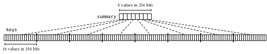
Figure 3. The node128 layout.

Queries are resolved as $\mbox{{sum}}(i)=\mbox{{summary}}[i/8]+\mbox{{keys}}[i]$. The code implementing update is given below.

⬇

void update(uint64_t i, bool sign) {

if (i == fanout) return;

uint64_t j = i / 16, k = i % 16;

__m256i s1 = _mm256_load_si256((__m256i const*)T_summary + j + sign * 8);

__m256i r1 = _mm256_add_epi32(_mm256_loadu_si256((__m256i const*)summary), s1);

_mm256_storeu_si256((__m256i*)summary, r1);

__m256i s2 = _mm256_load_si256((__m256i const*)T_segment + k + sign * 16);

__m256i r2 = _mm256_add_epi16(_mm256_loadu_si256((__m256i const*)(keys + j * 16)), s2);

_mm256_storeu_si256((__m256i*)(keys + j * 16), r2);

}

It uses two pre-computed tables. Precisely, T_summary stores $2\times 8\times 8$, 32-bit, signed integers, where $\mbox{{T\_summary}}[i][0..7]$ is an array whose first $i+1$ integers are 0 and the remaining $8-(i\bmod 8)-1$ are: $+1$ for $i=0..7$, and $-1$ for $i=8..15$. The table T_segment, instead, stores $2\times 16\times 16$, 16-bit, signed integers, where $\mbox{{T\_segment}}[i][0..15]$ is an array where the first $i$ integers are 0 and the remaining $16-(i\bmod 16)$ are: $+1$ for $i=0..15$, and $-1$ for $i=16..31$. The tables are used to obtain the register configuration that must be added to the summary and segment, respectively, regardless the sign of the update. (The difference with respect to the general approach by Pibiri and Venturini (2020a) is that tables can be used to directly obtain the register configuration to add because $\Delta$ is either $+1$ or $-1$ in this case, rather than a generic 64-bit value.)

Also note that the input parameter sign is 0 for $\Delta=+1$ and 1 for $\Delta=-1$, so that the use of update in the flip method of the mutable_bitmap class in Figure 1 (at page 1) is correct.

The $\mbox{{search}}(x)$ operation, that computes the smallest $i$ in $[0..128)$ such that $\mbox{{sum}}(i)>x$, can also be implemented using the SIMD instruction cmpgt (compare greater-than). Our approach is coded below, assuming that $x<\mbox{{sum}}(128-1)$.

⬇

std::pair<uint64_t, uint64_t> search(uint64_t x) const {

uint64_t i = 0;

__m256i cmp1 = _mm256_cmpgt_epi32(_mm256_loadu_si256((__m256i const*)summary),

_mm256_set1_epi32(x));

i = index_fs<32>(cmp1) - 1;

x -= summary[i];

i *= 16;

__m256i cmp2 = _mm256_cmpgt_epi16(_mm256_loadu_si256((__m256i const*)(keys + i)),

_mm256_set1_epi16(x));

i += index_fs<16>(cmp2);

return {i, i ? sum(i - 1) : 0};

}

The algorithm essentially uses parallel comparisons of $x$ against, first, the summary and, then, in a specific segment. The result of $\mbox{{cmpgt\_epi16}}(V,X)$ between the vectors $V$ and $X$ of 16-bit integers is a vector $Y$ such that $Y[i]=2^{16}-1$ if $V[i]>X[i]$ and 0 otherwise. From vector $Y$, we need to find the index of the “first set” (fs) 16-bit field. This function, referred to as index_fs in the code, can be implemented efficiently using the built-in instruction ctz (count trailing zeros) over 64-bit words. (The function takes a template parameter representing the number of bits of each integer in a 256-bit register.) Some notes are in order.

Note that, since $\mbox{{summary}}[0]=0$, it is guaranteed that index_fs(cmp1) is always at least 1 (but not necessarily true for index_fs(cmp2)).

As already mentioned, there is no cmpgt instruction for unsigned integers in instruction sets up to and including AVX2. Nonetheless, observe again that the search algorithm shown here is correct because we never use the 15-th bit (sign) of the 16-bit integers we load in the registers.

Lastly, observe that the search function returns a pair of integers, not only the index $i$ but also the sum of the elements to the “left of” index $i$ for convenience, i.e., $\mbox{{sum}}(i-1)$ (or just 0 if $i=0$), because this quantity is needed by the select operation in Figure 1.

Other node types. With node128 it is, therefore, possible to handle bitmaps of size up to $2^{7}B$ bits. We can now define a node64 structure, by applying the same design rules (and using similar algorithms) as we have done for the node128 structure. The node64 structure uses 8 segments, each holding 8 32-bit keys. Its summary array holds 32-bit numbers too. It follows that using a Segment-Tree of height two, where the root of the tree is a node of type node64 and its children are of type node128, it is possible ho handle bitmaps of size up to $2^{6+7}B$ bits. For a tree of height 3 we re-use again node64, for up to $2^{6+6+7}B$ bits. Adding another node, node32, made up of 4 64-bit values for the summary and segment of 8 32-bit keys, suffices to handle bitmaps of size up to $2^{24}B$ bits, e.g., $2^{32}$ bits for $B=256$. Table 2ba summarizes these node types, with Table 3ba showing how these are used in the Segment-Tree.

Table 2. Segment-Tree node types. The type nodex has fanout equal to x.

Type	Summary	Segment	Bytes
node32	4 $\times$ 64-bit	8 $\times$ 32-bit	160
node64	8 $\times$ 32-bit	8 $\times$ 32-bit	288
node128	8 $\times$ 32-bit	16 $\times$ 16-bit	288

(a) AVX2

Type	Summary	Segment	Bytes
node128	8 $\times$ 64-bit	16 $\times$ 32-bit	576
node256	16 $\times$ 32-bit	16 $\times$ 32-bit	1088
node512	16 $\times$ 32-bit	32 $\times$ 16-bit	1088

(b) AVX-512

Table 3. Segment-Tree configurations used to index a bitmap with blocks of $B$ bits, $B<2^{11}$.

Tree height	Node hierarchy	Bitmap size
4	node32	up to $2^{24}B$ bits
3	node64	up to $2^{19}B$ bits
2	node64	up to $2^{13}B$ bits
1	node128	up to $2^{7}B$ bits

(a) AVX2

Tree height	Node hierarchy	Bitmap size
3	node128	up to $2^{24}B$ bits
2	node256	up to $2^{17}B$ bits
1	node512	up to $2^{9}B$ bits

(b) AVX-512

5.2. Using AVX-512

Using registers of 512 bits clearly increases the parallelism of both updates and searches as $2\times$ more integers can be packed in a register compared to AVX2 that uses 256-bit registers. We can again define three node types to make full exploitation of the new AVX-512 instruction set: node512, node256, and node128. Their design is akin to that for AVX2 in the previous section, with details given in Table 2bb. Table 3bb shows, instead, that the height of the Segment-Tree can be reduced by 1 compared to AVX2. We also expect this to help in lowering the runtime as cache misses are reduced.

Another (minor) advantage of AVX-512 over AVX2 is that instructions implementing comparisons directly return a mask vector of 8, 16, 32, or 64 bits, instead of a wider SIMD register. This resulting mask can then be used as input for another instrinsic, such as ctz. In our case, the function index_fs used during a search operation just translates to one single ctz call (instead of 4 calls as in the case for a 256-bit register output by _mm256_cmpgt).

The only current limitation of AVX-512 is that is not as widespread as AVX2, so algorithms based on such instruction set are less portable.

5.3. Experimental Analysis

In this section, we measure the runtime of sum, update, and search, for the introduced Segment-Tree data structure and optimized state-of-the-art approaches, i.e., the Fenwick-Tree-based data structures described by Marchini and Vigna (2020), and implemented in the Sux (Vigna, 2020) C++ library. We reuse the nomenclature adopted by the authors in their own paper: Byte indicates compression at the byte granularity; Fixed indicates no compression; F stands for classic Fenwick layout; and L stands for level-order layout. For these experiments, we used arrays generated at random of size $2^{k}$ integers, for $k=8..24$. Since the runtime of the operations on the Segment-Tree does not depend on the block size $B$, we fix $B$ to 256 in these experiments. Therefore, each integer of the input array is a random value in $[0..256]$. (Each element of the array logically models the population count of a 256-bit block, so that the maximum array size cannot exceed $2^{24}$ for a bitmap of size $2^{32}$ bits.)

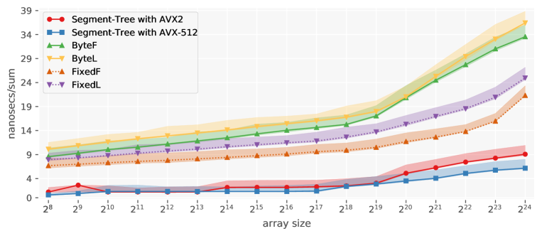
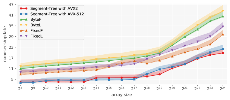
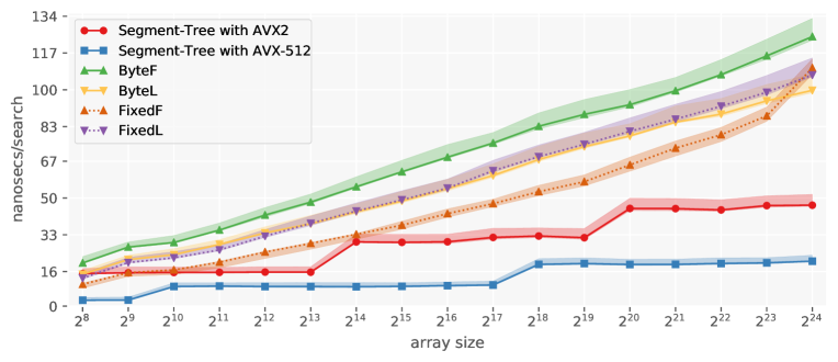
Figure 4. Average nanoseconds spent per operation by searchable prefix-sum data structures.

Figure 4 illustrates the result of the experiments. We shall first consider the Segment-Tree data structure described in this section and compare the use of AVX2 with AVX-512. The runtime of sum and update is very similar for both versions of the Segment-Tree. Recall that every tree operation translates into some of the corresponding operations performed at the nodes – one such operation per level of the tree. For sum and update, these node operations are data-independent and our implementation exploits this fact to leave the processor pipeline the opportunity to execute them out of order. Therefore, only one level of difference between the two tree heights does not suffice to make the two curves sufficiently distinct.

This consideration does not apply, instead, to the search operation because the result of search at level $\ell$ is used to perform search at level $\ell+1$, hence making the search algorithm inherently sequential. As a consequence of this fact, observe that the runtime of search is substantially higher than that of sum and update (not only because of the more complicated algorithm). In this case, the use of AVX-512 shines over AVX2 – often by a factor of $2\times$ – because one less level to traverse makes a big difference in the runtime of a sequential algorithm. (Also notice how both curves rise when one more level of the tree is in use.)

Compared to solutions based on the Fenwick-Tree, the Segment-Tree is consistently faster and by a good margin, confirming that the joint use of branch-free code and SIMD instructions have a significant impact on the practical performance of the data structures.

The space of the Segment-Tree is slightly more than the space needed to represent the input array itself, assuming that a fixed number of bytes is used to store each element. For our choice of block size, each array element can be stored in 2 bytes, so the number of bytes spent by the Segment-Tree for each element will be slightly more than 2 for sufficiently large inputs, i.e., $\approx$2.29 for AVX2 and $\approx$2.13 for AVX-512. In fact, the overhead of the tree hierarchy progressively vanishes as the tree height increases because nodes with large fanout are used. (It is easy to derive the exact number of bytes consumed by the data structure from the tree height and the space of each node type reported in Table 2b.) This ultimately means that, when the Segment-Tree is used as a bitmap index, its extra space is just $(2.29\times 8)/256\times 100\%<7.2\%$ of that of the bitmap itself with blocks of 256 bits, and less than 3.6% with blocks of 512 bits.

The compressed Fenwick-Tree data structures perform similarly to the Segment-Tree (the space for ByteF and ByteL is the same), taking $\approx$2 bytes per element. The Fixed variants take considerably more space because every element is represented with 4 or 8 bytes.

In conclusion, the searchable prefix-sum data structure described in this section – a Segment-Tree with SIMD-ized updates and searches – consumes space comparable to that of a compressed Fenwick-Tree while being significantly faster.

6. Rank/Select Queries over Small Bitmaps

In this section we study the problem of answering rank and select queries over small bitmaps of $B=256$ and 512 bits (four and eight 64-bit words respectively) without auxiliary space. We first describe the algorithms under a unifying implementation framework; then discuss experimental results to choose the fastest algorithms.

Table 4. The two-step framework for rank with approaches to perform the steps of (1) popcount and (2) prefix-sum.

broadword (Vigna, 2008, Alg. 1)

built-in instruction

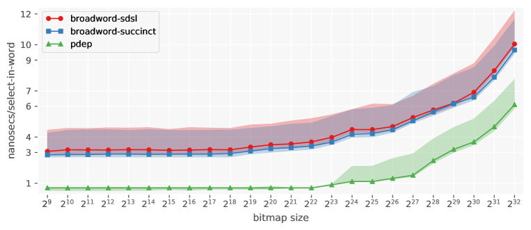
Figure 10. Average nanoseconds spent per select-in-word (step (3) in Table 53) by different algorithms.

SIMD (Muła et al., 2017, Figure 10)

(1) popcount

loop

unrolled loop

SIMD (Hillis and Steele, 1986, Figure 5 of this paper)

(2) prefix-sum

⬇

__m256i prefix_sum_256(__m256i C) {

static const int idx1 = _MM_SHUFFLE(2, 1, 0, 3);

static const int idx2 = _MM_SHUFFLE(1, 0, 3, 2);

C = _mm256_add_epi64(C, _mm256_maskz_permutex_epi64(0b11111110, C, idx1));

C = _mm256_add_epi64(C, _mm256_maskz_permutex_epi64(0b11111100, C, idx2));

return C;

}

__m512i prefix_sum_512(__m512i C) {

static const __m512i idx1 = _mm512_set_epi64(6, 5, 4, 3, 2, 1, 0, 7);

static const __m512i idx2 = _mm512_set_epi64(5, 4, 3, 2, 1, 0, 7, 6);

static const __m512i idx3 = _mm512_set_epi64(3, 2, 1, 0, 7, 6, 5, 4);

C = _mm512_add_epi64(C, _mm512_maskz_permutexvar_epi64(0b11111110, idx1, C));

C = _mm512_add_epi64(C, _mm512_maskz_permutexvar_epi64(0b11111100, idx2, C));

C = _mm512_add_epi64(C, _mm512_maskz_permutexvar_epi64(0b11110000, idx3, C));

return C;

}

Figure 5. A SIMD-based implementation of the parallel prefix-sum algorithm described by Hillis and Steele (1986), for 256 and 512 bits. It leverages the instructions maskz_permutex and maskz_permutexvar available in the instruction set AVX-512.

6.1. Rank

A common framework to solve rank for an index $0\leq i<B$ consists of the following two steps.

1. Count the numbers of ones appearing in the first $j=\lfloor{i/64}\rfloor$ words, where the $j$-th word is appropriately masked to zero the most significant $64-(i+1)\bmod 64$ bits.

2. Prefix-sum the resulting counters.

From a logical point of view, the result of step (1) is an array $C[0..B/64)$ of counters so that the final result for $\mbox{{rank}}(i)$ is computed as $C[0]+\dots+C[j]$ in step (2).

Several algorithms to perform these two steps are summarized in Table 42. By combining such basic steps we obtain different implementations of rank.

We have three different approaches to implement step (1). The first is the broadword algorithm by Vigna (2008, Algo. 1). The second is the __builtin_popcountll instruction available from SSE4.2. The third is a parallel algorithm using SIMD developed by Muła et al. (2017, Figure 10), to concurrently compute 4 or 8 popcount results, i.e., filling the vector $C$. (We took the original implementation made available by the authors at https://github.com/WojciechMula/sse-popcount.)

Also for step (2) we have three different approaches. The first is a simple loop that incrementally sums $C[k]$ for $0\leq k\leq j$, and requires a test for $j$ at each iteration. The second is an unrolled loop that computes all the prefix sums $C[k]=C[k]+C[k-1]$ for $0<k<B/64$ and returns $C[j]$. The approach does not require any branch. The third is a SIMD-based implementation of the parallel prefix-sum algorithm devised by Hillis and Steele (1986). In Figure 5 we show the two implementations for, respectively, 256 and 512 bits. Note that the last two approaches work in a branch-free manner but need to popcount all the $B/64$ words.

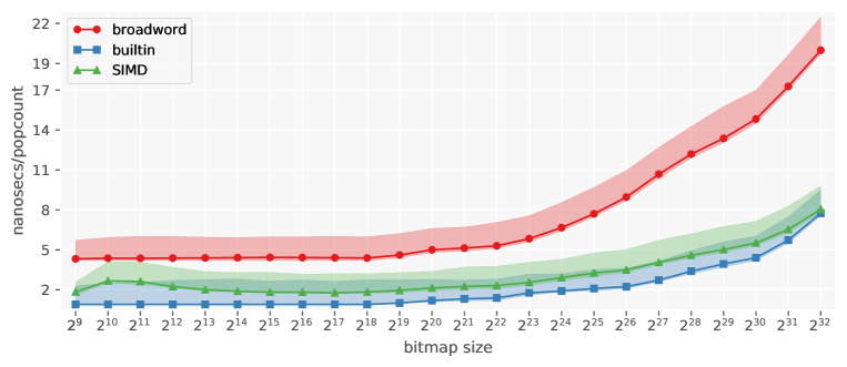
Figure 6. Average nanoseconds spent per pop-count (step (1) in Table 42) by different algorithms, for $B=256$. The trend for $B=512$ is the same, but the gap between broadword and the other approaches is more evident.

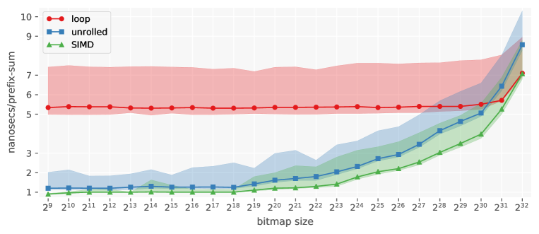
(a) $B=256$ bits

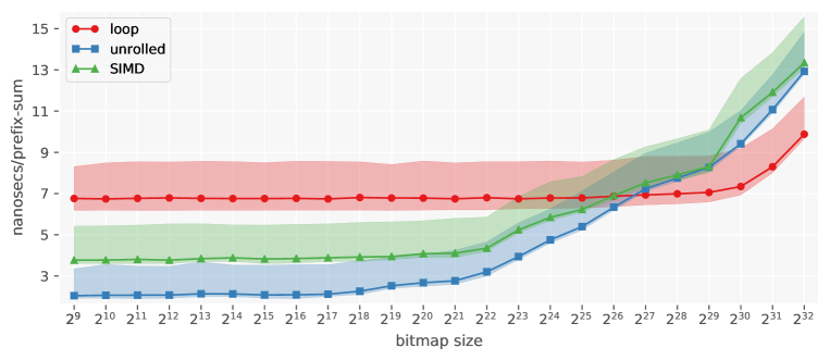
(b) $B=512$ bits

Figure 7. Average nanoseconds spent per prefix-sum (step (2) in Table 42) by different algorithms.

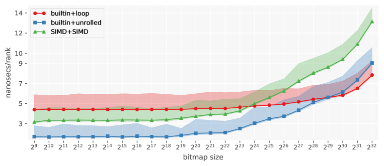
(a) $B=256$ bits

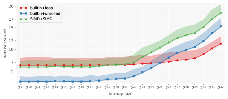
(b) $B=512$ bits

Figure 8. Average nanoseconds spent per rank by different algorithms.

We now consider the runtimes achieved by the various approaches reported in Table 42. For all such experiments, we generated random bitmaps of increasing size and random queries of the form $\langle j,i_{j}\rangle$, indicating that a given algorithm has to run over block $j$ and with index $i_{j}$ as input parameter.

Figure 6 shows the runtimes for step (1). The fastest approach is to use the built-in popcount instruction, with the SIMD-based algorithm catching up (especially on the larger $B=512$). The broadword algorithm is outperformed by the other two approaches. Concerning step (2), Figure 7 shows that the use of an unrolled loop provides consistently better results than a traditional loop for a wide range of practical bitmap sizes, because it completely avoids branches and increases the instruction throughput. It is comparable with (for $B=256$) or even better than SIMD (for $B=512$). However, when the size of a bitmap is very large, using a simple loop is faster. This is because large bitmaps involve slower memory accesses, resulting in the memory latency dominating the cost of the CPU pipeline flush. In that case, the branchy implementation becomes faster since unnecessary memory accesses are avoided. (In fact, the difference is more evident for the case $B=512$ rather than for $B=256$.) This is consistent with prior work (Pibiri and Venturini, 2020a).

Lastly, in the light of the results in Figure 6 and 7, we combine some of the approaches to obtain the fastest rank algorithm. Our expectation is that the combination builtin+unrolled performs best until the bitmap size becomes very large, when eventually the combination builtin+loop wins out. Also the implementation SIMD+SIMD is expected to be competitive with, but actually worse than, these two identified combinations. Figure 8 shows the runtimes of such algorithms and confirms our expectations.

6.2. Select

A common framework to solve select for an index $0\leq i<B$ consists of the following three steps.

1. Count the numbers of ones appearing in each word, using an array $C[0..B/64)$.

2. Prefix-sum $C$ and search for the $j$-th word, $w_{j}$, containing the $i$-th bit set.

3. Compute select locally in $w_{j}$, an operation that we denote by select64 (select-in-word).

More formally, step (2) determines the smallest $j$ such that $i<C[j]$ and step (3) returns $j64+\mbox{{select64}}(w_{j},i-C[j-1])$. Approaches to perform these steps are summarized in Table 53.

Table 5. The three-step framework for select with approaches to perform the steps of (1) popcount, (2) search, and (3) select-in-word.

same as in Table 42

(1) popcount

loop

SIMD

(2) search

broadword-sdsl (Gog and Petri, 2014, Sect. 6.2)

broadword-succinct (Vigna, 2008, Alg. 2)

parallel bits deposit (pdep) (Pandey et al., 2017)

(3) select-in-word

For step (1), we reuse the three approaches in Table 42 adopted for rank. For step (2), we have two approaches: the first is a simple loop that incrementally computes the prefix-sums in $C$ and checks if $i<C[j]$; the second is a branch-free implementation that computes the prefix-sums in parallel and finds the target $j$-th word using SIMD AVX-512 instructions. For step (3), we have three approaches. Two approaches are based on broadword programming, developed by Vigna (2008) and Gog and Petri (2014), respectively. We used the implementations available from the libraries Succinct (Grossi and Ottaviano, 2013) and Sdsl (Gog and Petri, 2014; Gog et al., 2014). (We took advantage of built-in instructions whenever possible. This makes both algorithms faster compared to when intrinsics are not used.) The third approach is a one-line algorithm using the parallel bits deposit (pdep) intrinsic devised by Pandey et al. (2017).

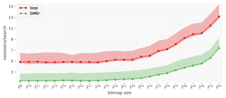
Figure 9. Average nanoseconds spent per search (step (2) in Table 53) by different algorithms, for $B=256$. (The shape for $B=512$ is the same.)

To benchmark the approaches in Table 53, we reuse the same methodology adopted for rank: random bitmaps of increasing size under a random workload of $\langle j,i_{j}\rangle$ queries. Answering $\mbox{{select}}(i_{j})$ over block $j$ makes the runtime practically independent from the density of the 1s, which we fixed to 30% in these experiments.

From the results in Figure 9 and 10, we see that SIMD is very effective in implementing the search step (which is also coherent with the results in Section 5) and the use of pdep is much faster than broadword approaches (as also noted in the paper by Pandey et al. (2017)).

As similarly done for rank, we now discuss some combinations of the basic steps to identify the fastest select algorithm. Since pdep is always the fastest at performing in-word-selection, we exclude broadword approaches. Clearly, we expect that a combination of SIMD+pdep for the last two steps performs best. The final result shown in Figure 11 again meets our expectations as the combination SIMD+SIMD+pdep is almost always the fastest. However, note that also the combination builtin+loop+pdep is good (and even the best for $B=512$ and large bitmaps) because the first two steps are inherently merged into one, i.e., popcount is performed within the searching loop, whereas the use of SIMD for step (2) requires computing popcount for all words. As already noticed, this performs fewer memory accesses that are very expensive for large bitmaps.

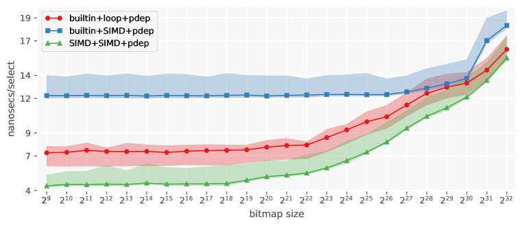
(a) $B=256$ bits

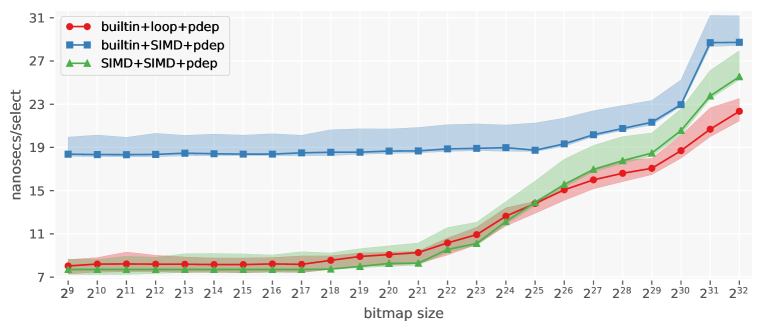
(b) $B=512$ bits

Figure 11. Average nanoseconds spent per select by different algorithms.

6.3. Conclusions

In the light of the experimental analysis in this section of the paper, we now summarize the two fastest algorithms for rank and select.

• For rank, use builtin+unrolled for all bitmaps of size up to $2^{25}$ bits (as a rule of thumb), and switch to builtin+loop for larger bitmaps.

• For select, use SIMD+SIMD+pdep if AVX-512 instructions are available, or builtin+loop+pdep otherwise.

We recall that we are going to use these selected algorithms over the blocks of a mutable bitmap data structure, as exemplified in Figure 1.

Now we report how much the runtime increases, in percentage, when considering these algorithms with $B=512$ compared to the case where $B=256$. To do so, we compute the average increase for three intervals of bitmap size $u$, that model small, medium, and large bitmaps respectively: (i) $2^{9}\leq u<2^{21}$, (ii) $2^{21}\leq u<2^{25}$, and (iii) $2^{25}\leq u\leq 2^{32}$. For rank, we determined an average increase of (i) 50%, (ii) 80%, and (iii) 40%. For select, we obtained (i) 80%, (ii) 80%, and (iii) 50%. These numbers show the doubling the block size $B$ sometimes causes the runtime to nearly double (+80%) as one would expect, but the increase is only 40-50% more on large bitmaps.

Lastly, we also conclude that SIMD instructions are more effective for select rather than rank. This is because potentially all words in the block must be searched, differently than rank that does not need any search, and this can be done quickly with SIMD.

7. Final Result

The mutable_bitmap class coded in Figure 1 (at page 1) can be tuned in many possible ways, depending on which index and rank/select algorithms are used to maintain its blocks. For the final examples we are going to illustrate in this section, we adopt the best results from the previous sections. (Other examples can be obtained by changing these two components.) Therefore, our tuning is summarized below.

As index, we use the $b$-ary Segment-Tree with SIMD AVX-512 described in Section 5, as this data structure gives the fastest results for search and preserves the runtime of sum/update compared to AVX2 (see Figure 4 at page 4). For rank in a block, we use the algorithm builtin+unrolled for all bitmap sizes up to $2^{25}$ and then switch to builtin+loop. We adopt this strategy for both $B=256$ and $B=512$. For select in a block, we use SIMD+SIMD+pdep for $B=256$ and builtin+loop+pdep for $B=512$. Rank and select in a single 64-bit word (i.e., $B=64$) are respectively done with masking followed by builtin popcount, and pdep.

With the indexing data structure and algorithms fixed, we show in Figure 12 the difference in runtime by varying the block size $B$. For all the experiments in this section, we use random bitmaps of increasing size, whose density is fixed to 0.3, under a random query workload (as consistently done in Section 6). The plots for flip and rank are very similar for all block sizes, thus the choice of $B=512$ should be preferred for the smaller space overhead. The impact of the block size is evident for select instead: increasing the block size makes the runtime to grow as well for different space/time trade-offs. In fact, we recall that our solution with blocks of 256 bits takes 7.2% extra space, and just 3.6% more with blocks of 512 bits. With the smallest block size, 64, the extra space becomes 26.7%.

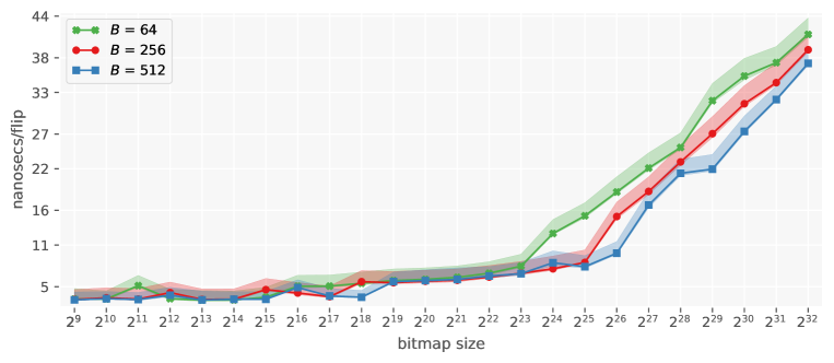
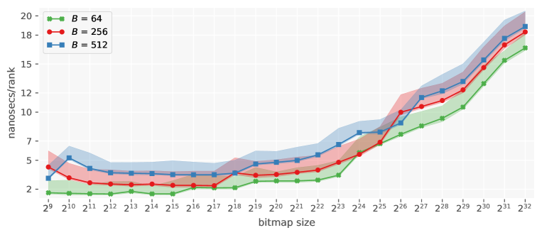
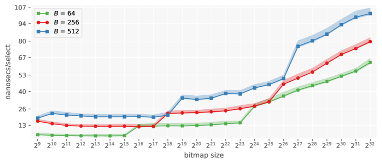
Figure 12. Average nanoseconds spent per operation by the mutable_bitmap by varying the block size $B=64,256,512$.

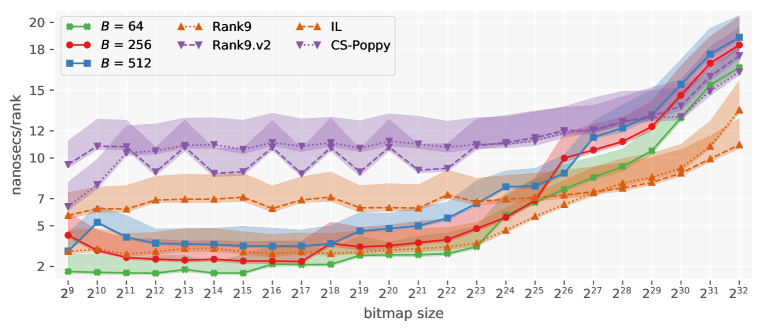
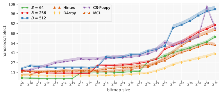
Figure 13. Average nanoseconds spent per operation by the mutable_bitmap by varying the block size ($B=64,256,512$), in comparison with other immutable indexes.

7.1. Comparison against Immutable Indexes

It is interesting to understand how our mutable index compares against the immutable indexes that we reviewed in Section 2.2, both in the uncompressed and compressed settings. This comparison is important to quantify how much the mutability feature impacts on the performance.

Uncompressed Indexes. Figure 13 reports the runtime of some selected uncompressed indexes in comparison with the mutable bitmap already shown in Figure 12. In order to choose our baselines, we take into account the following space/time trade-offs: (1) the most time-efficient solution that requires a separate index for each query; (2) the most time-efficient solution that requires a single index for both queries; and (3) the most space-efficient solution. For the first category, we have the combination Rank9+DArray. In this case, the extra space results from the sum of the space of the two indexes, which is at least 25% because of Rank9. We use the implementation available in the Succinct library. (The implementation of Rank9 in Sdsl performed the same as Succinct’s.) For the second category, we have the combination Rank9+Hinted that performs a binary search directly over the Rank9 index to solve select. Also in this case we use the Succinct’s implementation which only requires 3% extra space on top of Rank9, for a total of 28% extra. For the last category, we have Poppy with combined sampling (CS-Poppy), and we run the implementation by the original authors which requires 3.4% extra space to support both queries.

Other baselines available in the Sdsl library provide additional space/time trade-offs: Rank9.v2 is a more space-efficient version of Rank9 that takes $\approx$6% extra space; IL interleaves the original bitmap with rank informations to help locality of reference, taking 12.5% extra space; MCL is a modified Clark’s data structure for select, with low overhead (see Section 2.2 and Table 1b, page 1b).

From Figure 13 we see that the difference in runtime between our mutable index and the best immutable indexes is not as high as one would expect. Thus, our proposal brings further advantages in that it allows to modify the underlying bitmap without incurring in a significant runtime penalty and with even lower space overhead. More detailed observations are given below.

• Compared to the combination Rank9+DArray, the mutable index with $B=256$ only introduces a penalty in runtime for select on large bitmaps (from $2^{25}$ onward, by $2\times$), but takes several times less space. The extra space for Rank9 is fixed to 25% but the space of DArray depends on the density of the bitmap because it is a position-based solution. While we did not observe a meaningful difference in runtime by varying the density, we measured the space overhead for the densities $[0.1,0.3,0.5,0.7,0.9]$ and obtained $[5.6\%,16.9\%,28.1\%,39.4\%,50.6\%]$. Again, these should be summed to another 25%. Note that our mutable index does not depend on the density of the bitmap, therefore it consumes $4-11\times$ less space. Lastly, the efficiency gap for select can be reduced by using a smaller block size, e.g., $B=64$, with comparable or less space.

• Compared to the combination Rank9+Hinted, the mutable index with $B=256$ is basically as fast but also reduces the space overhead by $4\times$, from 28% to 7%.

• Compared to the most space-efficient index, CS-Poppy, the mutable index with $B=512$ is faster (especially for rank) and takes the same extra space.

• Concerning the implementations in the Sdsl library, we see that Rank9.v2 performs similarly to CS-Poppy but consumes more space; IL is $2\times$ more space-efficient than Rank9 but slower for small and medium sized bitmaps; MCL for select consumes less space than DArray but is consistently slower. It is also possible to binary search the IL layout to solve select but the runtime of this approach is $4-5\times$ slower than that of other approaches for medium and large bitmaps (therefore, we excluded it from the plots).

Compressed Indexes. We compare the mutable index with the compressed indexes proposed by Grabowski and Raniszewski (2018). (We recall that they aim at compressing the index component as well as the underlying bitmap. Refer to Section 2.2, page 2.2, for a description of their compressed layouts.) For consistency of presentation and methodology, we test the compressed indexes on random bitmaps of increasing size with density fixed to 0.3. As also shown by the original authors (see (Grabowski and Raniszewski, 2018, Figure 6)), the query time and space overhead of the compressed indexes is pretty much stable by varying the density of the bitmap (except possibly, for extremely sparse scenarios, i.e., 0.05 density). While we cannot expect a great deal of compression in this setting, our objective here is to determine the impact of a compressed layout on query time rather than that of saving space (indeed, recall that the mutable bitmap is not compressed).

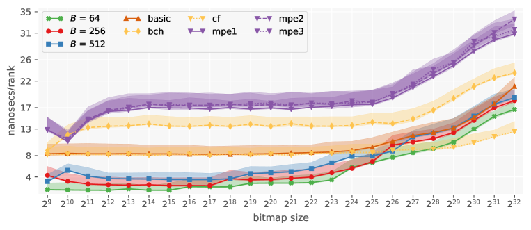
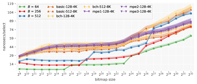
Figure 14. Average nanoseconds spent per operation by the mutable_bitmap by varying the block size ($B=64,256,512$), in comparison with other compressed indexes.

Figure 14 illustrates the comparison. We used the same names for the compressed indexes as given by the authors in their own paper (Grabowski and Raniszewski, 2018). (From Section 2.2, page 2.2, we recall that their indexes for select depend on two parameters, $\ell$ and $T$, that are also reported in Figure 14. For example, bch-128-4K indicates the bch layout with $\ell=128$ and $T=4096$.) The general trend is that a compressed layout can be faster than the mutable bitmap for large sizes (larger than, say, $2^{28}$ bits) because of a better cache exploitation. A more precise evaluation is as follows.

• Regarding the rank query, we determine a space overhead of: 25% for basic; 3.7% for bch; 12.5% for cf; and 4% for mpe1-3. Recall that the mutable index has an overhead of 26.7%, 7.2%, and 3.6%, for $B$ equal to 64, 256, and 512 respectively. The fastest compressed solution is cf (“cache friendly”), which is also faster than the mutable index on bitmap sizes larger than $2^{28}$ bits. Also, this variant always dominates the basic variant, being as fast or faster and with less space overhead. The other solutions, bch and mpe1-3, are consistently slower than the mutable bitmap.

• Regarding select instead, we determine a space overhead of: 31% for basic-128-4K; 7.6% for basic-512-8K; 20% for bch-128-4K; 5.1% for bch-512-8K; 20% for mpe-128-4K (1-3). In this case, the performance is quite similar for all the different compressed layouts on bitmaps up to $2^{26}$ bits, with the basic-128-4K variant being generally faster but with also the largest space overhead. On larger bitmaps, the compressed layouts are competitive with the mutable index for both $B=256$ and $B=512$.

As a last note, we remark that the compressed solutions we take into account here are optimized for one operation, i.e., the indexes for rank and different than those for select. This means that, as already pointed out for other immutable approaches, one has to build both indexes if both operations are needed for the same bitmap. The mutable index proposed in this article, instead, supports three operations (Rank, Select, and Flip) with the same data structure.

8. Conclusions and Future Work

We have proposed an efficient solution to the problem of rank/select queries over mutable bitmaps. The result leverages on the efficiency of two components: (1) a searchable prefix-sum data structure, optimized with SIMD instructions, and (2) rank/select algorithms over small immutable bitmaps. Comparison against the best immutable indexes reveals that a mutable index can be competitive in query time and consume even less space.

Future work will focus on making queries even faster, especially select that benefited more than rank from SIMD optimizations. Another study could explore the impact of compressing the blocks of the index for possibly improved space/time trade-offs in space-constrained applications.

9. Acknowledgments

The first author was partially supported by the BigDataGrapes (EU H2020 RIA, grant agreement N^o̱780751) and the OK-INSAID (MIUR-PON 2018, grant agreement N^o̱ARS01_00917) projects.

References

- (1)
- Bentley (1977) Jon Louis Bentley. 1977. Solutions to Klee’s rectangle problems. Unpublished manuscript (1977), 282–300.
- Bentley and Wood (1980) Jon Louis Bentley and Derick Wood. 1980. An optimal worst case algorithm for reporting intersections of rectangles. IEEE Trans. Comput. 7 (1980), 571–577.
- Brisaboa et al. (2014) Nieves R Brisaboa, Susana Ladra, and Gonzalo Navarro. 2014. Compact representation of web graphs with extended functionality. Information Systems 39 (2014), 152–174.
- Brisaboa et al. (2013) Nieves R Brisaboa, Miguel R Luaces, Gonzalo Navarro, and Diego Seco. 2013. Space-efficient representations of rectangle datasets supporting orthogonal range querying. Information Systems 38, 5 (2013), 635–655.
- Clark (1996) David Clark. 1996. Compact Pat Trees. Ph.D. Dissertation. University of Waterloo.
- Corporation (2020) Intel Corporation. [last accessed July 2020]. The Intel Intrinsics Guide, https://software.intel.com/sites/landingpage/IntrinsicsGuide.
- Fenwick (1994) Peter M. Fenwick. 1994. A new data structure for cumulative frequency tables. Software: Practice and experience 24, 3 (1994), 327–336.
- Ferragina et al. (2009) Paolo Ferragina, Rodrigo González, Gonzalo Navarro, and Rossano Venturini. 2009. Compressed text indexes: From theory to practice. Journal of Experimental Algorithmics (JEA) 13 (2009), 1–12.
- Fredman and Saks (1989) Michael Fredman and Michael Saks. 1989. The cell probe complexity of dynamic data structures. In Proceedings of the 21st Annual Symposium on Theory of Computing (STOC). 345–354.
- Gog et al. (2014) Simon Gog, Timo Beller, Alistair Moffat, and Matthias Petri. 2014. From theory to practice: Plug and play with succinct data structures. In Proceedings of the 13th International Symposium on Experimental Algorithms (SEA). Springer, 326–337.
- Gog and Petri (2014) Simon Gog and Matthias Petri. 2014. Optimized succinct data structures for massive data. Software: Practice and Experience 44, 11 (2014), 1287–1314.
- Golynski (2007) Alexander Golynski. 2007. Optimal lower bounds for rank and select indexes. Theoretical Computer Science 387, 3 (2007), 348–359.
- González et al. (2005) Rodrigo González, Szymon Grabowski, Veli Mäkinen, and Gonzalo Navarro. 2005. Practical implementation of rank and select queries. In Poster Proceedings of the 4th Workshop on Experimental and Efficient Algorithms (WEA). 27–38.
- Grabowski and Raniszewski (2018) Szymon Grabowski and Marcin Raniszewski. 2018. Rank and select: Another lesson learned. Information Systems 73 (2018), 25–34.
- Grossi and Ottaviano (2013) Roberto Grossi and Giuseppe Ottaviano. 2013. Design of practical succinct data structures for large data collections. In Proceedings of the 12th International Symposium on Experimental Algorithms (SEA). Springer, 5–17.
- Hillis and Steele (1986) W. Daniel Hillis and Guy L. Steele. 1986. Data parallel algorithms. Commun. ACM 29, 12 (Dec. 1986), 1170–1183.
- Jacobson (1988) Guy Joseph Jacobson. 1988. Succinct static data structures. Ph.D. Dissertation. Carnegie Mellon University.
- Kanda et al. (2017) Shunsuke Kanda, Kazuhiro Morita, and Masao Fuketa. 2017. Practical string dictionary compression using string dictionary encoding. In Proceedings of the 3rd International Conference on Big Data Innovations and Applications (Innovate-Data). 1–8.
- Marchini and Vigna (2020) Stefano Marchini and Sebastiano Vigna. 2020. Compact Fenwick trees for dynamic ranking and selection. Software: Practice and Experience 50, 7 (2020), 1184–1202.
- Martínez-Prieto et al. (2016) Miguel A Martínez-Prieto, Nieves Brisaboa, Rodrigo Cánovas, Francisco Claude, and Gonzalo Navarro. 2016. Practical compressed string dictionaries. Information Systems 56 (2016), 73–108.
- Miltersen (2005) Peter Bro Miltersen. 2005. Lower bounds on the size of selection and rank indexes. In Proceedings of the 16th Annual ACM-SIAM Symposium on Discrete Algorithms (SODA), Vol. 23. Citeseer, 11–12.
- Muła et al. (2017) Wojciech Muła, Nathan Kurz, and Daniel Lemire. 2017. Faster population counts using AVX2 instructions. Comput. J. 61, 1 (2017), 111–120.
- Navarro and Providel (2012) Gonzalo Navarro and Eliana Providel. 2012. Fast, small, simple rank/select on bitmaps. In Proceedings of the 11th International Symposium on Experimental Algorithms (SEA). Springer, 295–306.