Modelling neutron star mountains

Abstract

As the era of gravitational-wave astronomy has well and truly begun, gravitational radiation from rotating neutron stars remains elusive. Rapidly spinning neutron stars are the main targets for continuous-wave searches since, according to general relativity, provided they are asymmetrically deformed, they will emit gravitational waves. It is believed that detecting such radiation will unlock the answer to why no pulsars have been observed to spin close to the break-up frequency. We review existing studies on the maximum mountain that a neutron star crust can support, critique the key assumptions and identify issues relating to boundary conditions that need to be resolved. In light of this discussion, we present a new scheme for modelling neutron star mountains. The crucial ingredient for this scheme is a description of the fiducial force which takes the star away from sphericity. We consider three examples: a source potential which is a solution to Laplace’s equation, another solution which does not act in the core of the star and a thermal pressure perturbation. For all the cases, we find that the largest quadrupoles are between a factor of a few to two orders of magnitude below previous estimates of the maximum mountain size.

1 Introduction

Neutron stars have long been of interest in gravitational-wave astronomy (Papaloizou & Pringle, 1978; Wagoner, 1984). This is owed to their extreme compactness (rivalled only by black holes) and their role in some of the most cataclysmic events in the Universe. There are a variety of mechanisms through which neutron stars can radiate gravitational waves. These include binary inspiral and merger (Abadie et al., 2010), various modes of oscillation (and their corresponding instabilities; Andersson, 1998; Andersson, Kokkotas & Stergioulas, 1999) and rotating neutron stars deformed away from axial symmetry (Bildsten, 1998). Recently, binary neutron stars have been the subject of significant interest since their exciting, first detections with gravitational-wave interferometers (Abbott et al., 2017d, 2020b). This has reinvigorated the effort to explore other neutron star gravitational-wave scenarios.

An open problem in the study of spinning neutron stars relates to the fact that no neutron star has been observed that spins (even remotely) close to the centrifugal break-up frequency – which is generally above $\sim$1\text{\,}\mathrm{kHz}$$ for most equation-of-state candidates (Lattimer & Prakash, 2007). The fastest discovered spinning pulsar rotates at $716\text{\,}\mathrm{Hz}$ (Hessels et al., 2006), well below this mass-shedding limit, and the current theory predicts that these stars reach these high frequencies through accretion, which should have no difficulty in spinning the neutron stars up to this limit (Cook, Shapiro & Teukolsky, 1994). It has been suggested that the lack of neutron stars spinning at these high rates is due to the emission of gravitational radiation which provides a braking torque that halts spin-up (Bildsten, 1998; Andersson et al., 1999; Gittins & Andersson, 2019). The associated (quadrupole) deformations are commonly referred to as mountains.

Rapidly rotating neutron stars have, in fact, enjoyed the attention of a large number of searches using gravitational-wave data. These searches have been split into two strategies: looking for evidence of gravitational radiation for specific pulsars (Abbott et al., 2004, 2005b, 2007a, 2008b, 2010; Abadie et al., 2011a, b; Aasi et al., 2014, 2015a, 2015b; Abbott et al., 2017a, c, e, f, 2018b, 2019a, 2019e, 2019b) and wide-parameter surveys for unobserved sources (Abbott et al., 2005a, 2007b, 2008a, 2009; Abadie et al., 2012; Aasi et al., 2013; Abbott et al., 2016, 2017b, 2018a). There has also been a study looking for gravitational waves from supernova remnants (Abbott et al., 2019d). The recent wide-parameter search (Abbott et al., 2019c) has excluded the presence of fast-spinning neutron stars within $100$ parsecs with ellipticities larger than $10^{-8}$ and, most recently, the ellipticities of a number of observed pulsars have been constrained to less than $10^{-8}$ (Abbott et al., 2020a). For these reasons, it is of great interest to calculate the largest mountain that a neutron star crust can sustain. This would provide an upper limit on the magnitude of gravitational-wave emission from these systems.

There have been a number of studies of the maximum quadrupole deformation of a neutron star. The earliest of these was conducted by Ushomirsky, Cutler & Bildsten (2000), who used the Cowling approximation in Newtonian gravity to derive an integral expression for the quadrupole moment. They introduced the argument that the body will obtain its maximum mountain when the crust is strained to its elastic yield point. This argument enabled them to straightforwardly find the strain tensor that ensures that every point in the crust is maximally strained. Haskell, Jones & Andersson (2006) observed that the approach of Ushomirsky et al. (2000) did not respect the required boundary conditions at the base and top of the crust and that the Cowling approximation could have a large impact on the results. Therefore, they presented a perturbation formalism that relaxed the Cowling approximation and enabled them to treat the phase transitions appropriately. However, there are inconsistencies in their analysis which we explain later. The most recent estimates of the maximum elastic deformation have been provided by Johnson-McDaniel & Owen (2013), who carried out their calculation in full relativity using a Green’s function method. However, since they used the covariant analogue to the strain tensor from Ushomirsky et al. (2000), their calculation also ignored the boundary conditions on the crust. An important aspect of past studies is the fact the maximum mountains they calculate are independent of the precise mechanisms which sourced them. They do not consider the deforming forces or evolutionary scenarios which lead to the formation of the mountains.

We return to this problem to address some of the assumptions of the previous work and detail a formalism which enables one to accurately compute the quadrupole deformation throughout the star. As we show, in order to satisfy the necessary boundary conditions of the problem, it is extremely helpful to characterise the source of the perturbations. This has not been done in past calculations. In addition, it is not clear whether strain configurations where the majority of the crust is maximally strained can actually be reached in a real neutron star. The largest realistic mountain may be significantly smaller. These points suggest that future progress on this subject will rely on evolutionary calculations that consider the complete formation of the mountains (Bildsten, 1998; Ushomirsky et al., 2000; Singh et al., 2020; Osborne & Jones, 2020).

We begin, in Section 2, with an introduction to static perturbations of neutron stars and a review of prior efforts on estimating the maximum mountain. We summarise their approaches and the important assumptions, which provide the motivation for this work. In Section 3, we consider the necessary components of a neutron star mountain calculation. We provide a detailed discussion on the usual method of calculating mountains and introduce our own scheme, demonstrating the validity and equivalence of both approaches. We detail the perturbation formalism for our mountain scheme in Section 4 and pay particular attention to the boundary conditions of the problem. We consider three sources for the deformations in Section 5 and provide the maximum quadrupoles for each scenario. Finally, we conclude and discuss future work in Section 6.

We adopt the usual Einstein summation convention where repeated indices indicate a summation. We use Latin characters $i,j,...$ to denote spatial indices and use primes for derivatives with respect to the radial coordinate. We use $\delta$ and $\Delta$ to represent Eulerian and Lagrangian perturbations, respectively. These perturbations are related by $\Delta=\delta+\mathcal{L}_{\xi}$, where $\mathcal{L}_{\xi}$ is the Lie derivative along the Lagrangian displacement vector, $\xi^{i}$ (Friedman & Schutz, 1978).

2 Context

When a star is deformed away from perfect sphericity it develops multipole moments. These are defined as

$$Q_{lm}\equiv\int_{0}^{R}\delta\rho_{lm}(r)r^{l+2}dr,$$ (1)

where $(l,m)$ denotes the harmonic mode of the density perturbation, $\delta\rho_{lm}(r)$, and $R$ is the stellar radius. Note, in order to describe the full perturbative behaviour one would need to evaluate the sum over all modes, $\delta\rho(r,\theta,\phi)=\sum_{l=0}^{\infty}\sum_{m=-l}^{l}\delta\rho_{lm}(r)Y_{lm}(\theta,\phi)$, where $Y_{lm}(\theta,\phi)$ are the usual spherical harmonics. However, since we are considering the quadrupole moment, $Q_{22}$, which is the dominant multipole in gravitational-wave emission, it is sufficient for the analysis to focus on the $(l,m)=(2,2)$ mode. For this reason, we will drop the mode subscript on our perturbation variables.

In addition to the quadrupole moment, we will quote our results using the fiducial ellipticity (Owen, 2005),

$$\epsilon=\sqrt{\frac{8\uppi}{15}}\frac{Q_{22}}{I_{zz}},$$ (2)

where $I_{zz}$ is the principal stellar moment of inertia, which we take to have the fiducial value of $I_{zz}=${10}^{45}\text{\,}\mathrm{g}\text{\,}{\mathrm{cm}}^{2}$$. We do this to facilitate comparisons with observational papers.

In this paper, we restrict ourselves to Newtonian gravity. Because of this, it is inappropriate to consider realistic equations of state and we assume a simple polytropic equation of state (Section 5).

We consider perturbations of a non-rotating, fluid star with mass density $\rho$, isotropic pressure $p$ and gravitational potential $\Phi$. A barotropic fluid configuration, with velocity $v^{i}$, is a solution $(\rho,p,v^{i})$ to the following equations:

$$\partial_{t}\rho+\nabla_{i}(\rho v^{i})=0,$$ (3)

$$\rho(\partial_{t}+v^{j}\nabla_{j})v_{i}=-\nabla_{i}p-\rho\nabla_{i}\Phi,$$ (4)

$$p=p(\rho)$$ (5)

and the gravitational potential is provided by Poisson’s equation,

$$\nabla^{2}\Phi=4\uppi G\rho.$$ (6)

Since the star is in equilibrium, the time derivatives vanish and, because it is static, we set $v^{i}=0$ – which means the continuity equation (3) is trivially satisfied.

To capture how the fluid elements move due to an induced perturbation, we introduce the Lagrangian displacement vector, $\xi^{i}$. This is related to the Lagrangian perturbation of the velocity (Friedman & Schutz, 1978),

$$\Delta v^{i}=\partial_{t}\xi^{i}.$$ (7)

The equations which govern the perturbations in a fluid are obtained by considering variations of equations (3)–(6). For a static background, $\delta v^{i}=\Delta v^{i}=\partial_{t}\xi^{i}$ and we have

$$\delta\rho+\nabla_{i}(\rho\xi^{i})=0,$$ (8)

$$\rho\partial_{t}^{2}\xi_{i}=-\nabla_{i}\delta p-\delta\rho\nabla_{i}\Phi-\rho\nabla_{i}\delta\Phi,$$ (9)

$$\delta p=c_{\text{s}}^{2}\delta\rho$$ (10)

and

$$\nabla^{2}\delta\Phi=4\uppi G\delta\rho,$$ (11)

where $c_{\text{s}}^{2}\equiv dp/d\rho$ is the squared sound speed. Since we focus on static perturbations, we amend the perturbed Euler equation (9) by

$$0=-\nabla_{i}\delta p-\delta\rho\nabla_{i}\Phi-\rho\nabla_{i}\delta\Phi+f_{i},$$ (12)

where $f_{i}$ is the density of a force which sustains the perturbations. The inclusion of this force enables us to produce non-spherical models and will prove to be an important component of our analysis, since it enables one to satisfy all the boundary conditions of the problem. We note that $f_{i}$ does not correspond to a physical force acting on the star. This force is a proxy for the (possibly quite complicated) formation history that results in its non-spherical shape. To study neutron stars with an elastic crust, we must modify (12) to include the shear stresses,

$$0=-\nabla_{i}\delta p-\delta\rho\nabla_{i}\Phi-\rho\nabla_{i}\delta\Phi+\nabla^{j}t_{ij}+f_{i},$$ (13)

where $t_{ij}$ is the shear-stress tensor, assumed to enter at the perturbative level. Here, we have used the same sign for the shear-stress tensor as in Ushomirsky et al. (2000).

As we discuss in detail in Section 4.3, in order to connect the elastic crust of the star with the fluid regions, one needs to consider the traction vector. This must be continuous throughout the star.

We turn our attention to past work on estimating the maximum mountain, which we now summarise. We do this to critique some of the assumptions made and set the stage for our new calculation. A convenient simplification that this body of work makes is to not (explicitly) consider the perturbing force. This is the main conceptual difference in our approach. We show how the force enters the problem in Section 3 and demonstrate that the formulation is consistent.

2.1 Ushomirsky, Cutler & Bildsten

The first (and perhaps most well known) maximum-mountain calculation was performed by Ushomirsky et al. (2000). They tackled the problem in Newtonian gravity and adopted the Cowling approximation – neglecting perturbations of the star’s gravitational potential, $\delta\Phi=0$. The Cowling approximation means one can ignore perturbations in the fluid regions of the star, since the absence of shear stresses means there is no support for the pressure perturbations by the fluid [see (12) with $f_{i}=0$]. Therefore, only perturbations in the crust contribute to the quadrupole moment.

As is the current standard approach, Ushomirsky et al. (2000) assumed that the crust manifests itself only at the perturbative level and, therefore, does not affect the equilibrium structure. From the perturbed Euler equation for an elastic solid [(13) with $f_{i}=0$], they obtained an integral expression for the quadrupole moment of the star which depends on the shear stresses in the crust. In order to find an expression for these stresses, they conjectured that a star will attain its maximum quadrupole deformation when the crust is strained everywhere to the breaking point. To define the elastic yield limit, Ushomirsky et al. (2000) used the von Mises criterion and further assumed that all the strain is in the $(l,m)=(2,2)$ multipole. Thus, they analytically obtained the strain tensor which corresponds to the star being maximally strained.

For a star with mass $M=$1.4\text{\,}\mathrm{\mbox{$M_{\odot}$}}$$ and radius $R=$10\text{\,}\mathrm{km}$$, Ushomirsky et al. (2000) reported a maximum quadrupole moment of

$$Q_{22}^{\text{max}}\approx$1.2\text{\times}{10}^{39}$\ \left(\frac{\bar{\sigma}_{\text{max}}}{10^{-1}}\right)\ $\mathrm{g}\text{\,}{\mathrm{cm}}^{2}$,$$ (14)

where $\bar{\sigma}_{\text{max}}$ is the breaking strain of the crust, which we take to have the canonical value, $\bar{\sigma}_{\text{max}}=10^{-1}$ (Horowitz & Kadau, 2009). In terms of the fiducial ellipticity, this result corresponds to $\epsilon^{\text{max}}\approx$1.6\text{\times}{10}^{-6}$\ (\bar{\sigma}_{\text{max}}/10^{-1})$.

This approach, while elegant, does not enforce the continuity of the traction vector at the boundaries of the crust. At the base of the crust, there is a transition between the fluid core and the elastic crust. At the top, there is a transition between the elastic region and the fluid ocean. At these interfaces, there is expected to be a first-order phase transition where the crust sharply obtains a non-zero shear modulus. Since the fluid has a vanishing shear modulus, the traction can only be continuous if the appropriate strain components go to zero at these boundaries. However, due to the fact that Ushomirsky et al. (2000) demanded that the crust be maximally strained at every point, the strain components have finite values at the interfaces and, therefore, one cannot ensure continuity of the traction.

In defence of the Ushomirsky et al. (2000) approach, one might argue that the shear modulus may be assumed to smoothly go to zero at the phase transitions. However, this is still problematic. As we show in Section 4.3, such an assumption means that one does not have enough equations to uniquely determine the displacement, in the case where one does not know the strain. A more realistic assumption might be to take almost the entire crust to be at breaking strain, with the exception of an infinitesimally small region at the boundaries where the displacement is adjusted to satisfy the continuity of the traction.

Ultimately, the estimate (14) may give us an idea of the likely maximum mountain, but the calculation is not completely consistent.

2.2 Haskell, Jones & Andersson

Haskell et al. (2006) set out to relax some of the assumptions made by Ushomirsky et al. (2000). This included dropping the Cowling approximation and ensuring the traction is continuous at the appropriate boundaries. They also noted that, by insisting the star is strained to the maximum throughout the crust, one loses the freedom to impose the boundary conditions of the problem.

Haskell et al. (2006) derived a system of coupled ordinary differential equations which describe the perturbations in the elastic crust and the fluid core relative to a spherically symmetric background star. They numerically integrated the perturbation equations and fixed the perturbation amplitude to the maximum necessary to begin to break the crust at a point, according the von Mises criterion. In their study, Haskell et al. (2006) obtained the largest mountain when they assumed the core to be unperturbed, thus, allowing them to use a fully relativistic core combined with Newtonian perturbations in the crust. They reported a maximum quadrupole for a star with $M=$1.4\text{\,}\mathrm{\mbox{$M_{\odot}$}}$$, $R=$10\text{\,}\mathrm{km}$$ of

$$Q_{22}^{\text{max}}\approx$3.1\text{\times}{10}^{40}$\ \left(\frac{\bar{\sigma}_{\text{max}}}{10^{-1}}\right)\ $\mathrm{g}\text{\,}{\mathrm{cm}}^{2}$,$$ (15)

which corresponds to an ellipticity of $\epsilon^{\text{max}}\approx$4.0\text{\times}{10}^{-5}$\ (\bar{\sigma}_{\text{max}}/10^{-1})$. This result is approximately an order of magnitude above that of Ushomirsky et al. (2000).

The calculation of Haskell et al. (2006) correctly treated the boundary condition at the crust-core interface by demanding that the traction was continuous. However, their calculation assumed the relaxed shape – the strain is taken with respect to – to be spherical. In general, the relaxed shape must be non-spherical, to give an equilibrium solution with a non-zero mountain. They did however stipulate that the surface shape of the star was deformed in an $(l,m)=(2,2)$ way. This effectively meant using an outer boundary condition where a traction-like force (i.e., a force per unit area) acts at the very surface of the star. Because of this, the maximum quadrupoles calculated in this framework turn out to be insensitive to the shear modulus of the crust, as they are sustained by this applied surface force. The lack of inclusion of a body force (i.e., a force per unit volume) in building the mountain meant that their formalism did not have the necessary freedom to ensure that the perturbed potential in the interior matches to the exterior solution. We discuss this particular subtlety further in Section 4.1.

By comparing with our new analysis we also note a number of typographical errors in their elastic perturbation equations. These errors turn out to have a surprisingly dramatic effect. Once they are corrected the maximum quadrupole increases by three orders of magnitude, in sharp contrast with other estimates. This, in turn, highlights the conceptual problem with the formulation.

2.3 Johnson-McDaniel & Owen

The most recent estimates for the largest possible mountain on a neutron star were provided by Johnson-McDaniel & Owen (2013). They generalised the Ushomirsky et al. (2000) argument to relativistic gravity while relaxing the Cowling approximation. They evaluated the required integral by employing a Green’s function. For a $1.4\text{\,}\mathrm{\mbox{$M_{\odot}$}}$ star, described by the SLy equation of state (Douchin & Haensel, 2001), they obtained the result,

$$Q_{22}^{\text{max}}\approx$2\text{\times}{10}^{39}$\ \left(\frac{\bar{\sigma}_{\text{max}}}{10^{-1}}\right)\ $\mathrm{g}\text{\,}{\mathrm{cm}}^{2}$,$$ (16)

corresponding to $\epsilon^{\text{max}}\approx$3\text{\times}{10}^{-6}$\ (\bar{\sigma}_{\text{max}}/10^{-1})$.

In following the Ushomirsky et al. (2000) approach, the crust was taken to be strained to the maximum at every point, which means that the traction vector cannot be continuous at the crust boundaries. Furthermore, they do not use the correct expression for the perturbed stress-energy tensor, since it does not include variations of the four-velocity. This may be a minor detail, but it should still be noted.

In summary, although some of the above points may have a negligible impact on the maximum quadrupole estimates, there are issues with all previous studies of the maximum-mountain problem.

3 Building mountains

In this section, we examine what must go into a consistent mountain calculation and discuss two methods for modelling mountains on neutron stars. The first approach, introduced in Ushomirsky et al. (2000), involves specifying the strain field associated with the mountain. We present a second method which, instead of starting with the strain, starts with a description of the perturbing force. Both approaches are valid and we demonstrate how they are equivalent.

To help develop intuition, we will start by briefly discussing the case of strains built up in a spinning down star. We will therefore be considering the case of $(l,m)=(2,0)$ perturbations relevant for rotational deformations, not the $(l,m)=(2,2)$ relevant to the mountain case. Suppose a young neutron star with a molten crust spins at an angular frequency, $\Omega$. At this rotation rate, the star cools and the crust solidifies. The star then begins to spin down to frequency, $\tilde{\Omega}<\Omega$. Because the star has spun down, it changes shape according to the difference in the centrifugal force, $\propto(\Omega^{2}-\tilde{\Omega}^{2})$. This builds up strain in the crust as the shear stresses resist the change in shape. Should the star spin down sufficiently, the crust may fracture as stresses get too large. In fact, it has been suggested that the elastic yield of the crust in this process may be associated with the glitch phenomenon observed in some rotating pulsars (Baym & Pines, 1971; Keer & Jones, 2015).

Motivated by this example, which does not represent a neutron star mountain, we consider neutron star models forced away from sphericity by a perturbing force $f_{i}$, which we will choose to give mountain-like $(l,m)=(2,2)$ perturbations. The elastic Euler equation (13) then becomes

$$0=-\nabla_{i}p-\rho\nabla_{i}\Phi+\nabla^{j}t_{ij}+f_{i},$$ (17)

We regard this equation as exact, and will consider perturbations of it below. In the fluid regions of the star, which cannot support shear stresses, the shear modulus goes to zero so the shear-stress tensor vanishes. To condense the notation, we define

$$H_{i}\equiv\nabla_{i}p+\rho\nabla_{i}\Phi,$$ (18)

which captures the familiar equation of hydrostatic equilibrium when $H_{i}=0$. Therefore, the Euler equation (17) can be expressed as

$$H_{i}=f_{i}+\nabla^{j}t_{ij}.$$ (19)

By considering a variation of $H_{i}$, we may write

$$\delta H_{i}=\nabla_{i}\delta p+\delta\rho\nabla_{i}\Phi+\rho\nabla_{i}\delta\Phi,$$ (20)

where the perturbed quantities will need to be carefully defined in what follows.

We now consider a family of four closely-related, equilibrium stars, illustrated in Fig. 1:

• Star S – A spherical, fluid star with $(\rho_{\text{S}},p_{\text{S}},\Phi_{\text{S}})$:

  $$H_{i}^{\text{S}}=0.$$ (21)

• Star A – A force is applied to star S, which produces a non-spherical, fluid star with $(\rho_{\text{A}},p_{\text{A}},\Phi_{\text{A}})$:

  $$H_{i}^{\text{A}}=f_{i}.$$ (22)

• Star à – The crust of star A solidifies while the force is maintained. This gives rise to a non-spherical, relaxed star with the same structure as star A, although (formally) with a non-zero shear modulus. The star has $(\rho_{\text{\~{A}}}=\rho_{\text{A}},p_{\text{\~{A}}}=p_{\text{A}},\Phi_{\text{\~{A}}}=\Phi_{\text{A}})$:

  $$H_{i}^{\text{\~{A}}}=H_{i}^{\text{A}}=f_{i}.$$ (23)

  Note that, because star A and star à have the same shape, in general, we only need to refer to star A in the following discussion when specifying the values of perturbed quantities.

• Star B – The force on star à is removed, which builds up strain in the crust. The associated deformation between these two stars is described by the Lagrangian displacement vector field, $\eta^{i}$. The star is non-spherical and strained with $(\rho_{\text{B}},p_{\text{B}},\Phi_{\text{B}})$:

  $$H_{i}^{\text{B}}=\nabla^{j}t_{ij}(\eta).$$ (24)

  Note that it is this star, star B, that we are ultimately interested in: this is the star with a mountain supported in a self-consistent way by elastic strains, with no external force acting.

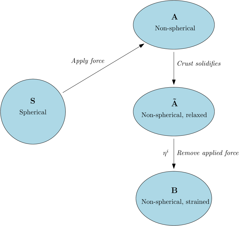
Figure 1: A schematic illustration showing the configurations involved in mountain calculations. Note that previous calculations have typically considered stars S and B, but not (explicitly) A or Ã.

Note that the force $f_{i}$ has a simple physical interpretation: it is the force that, when applied to our equilibrium star with the mountain (star B), takes us to the corresponding unstrained star (star A, or equivalently Ã). Note, however, that there is no requirement whatsoever that, in the real world, this force ever acted upon our star. For a realistic situation, the elastic strains that support the deformation of star B will likely have evolved through some complex process of plastic flow and cracking, possibly combined with whatever agent causes the asymmetry to develop. The usefulness of $f_{i}$ is two-fold. Firstly, it allows us to explicitly identify the unstrained configuration. Secondly, the explicit introduction of the force into the Euler equation provides the necessary freedom to determine the displacement vector and satisfy all the boundary conditions.

It is useful to consider the differences between the stellar models described above. Thus, we introduce the notation,

$$\delta H_{i}^{\text{AB}}=H_{i}^{\text{B}}-H_{i}^{\text{A}},$$ (25)

i.e., $\delta H_{i}^{\text{AB}}$ is the quantity that must be added to $H_{i}^{\text{A}}$ to obtain $H_{i}^{\text{B}}$.

The difference between star B (24) and star S (21) is

$$\delta H_{i}^{\text{SB}}=\nabla^{j}t_{ij}(\eta).$$ (26)

Expression (26) relates perturbations between the strained star – with a mountain – and the spherical, reference star to the shear stresses induced when the relaxed star is deformed according to the displacement, $\eta^{i}$. This is the standard picture for understanding neutron star mountains and, indeed, it is this expression that is used to estimate the maximum quadrupole in Ushomirsky et al. (2000) and Johnson-McDaniel & Owen (2013). It is important to note that in these calculations one does not have to determine the relaxed shape and, indeed, stars A and à did not appear explicitly in previous calculations. However, we demonstrate that the relaxed shape is, in principle, calculable in Appendix A.

As we discuss in more detail below, for a fully consistent calculation that satisfies all the boundary conditions of the problem it is not convenient to use (26) alone. Rather, we present an alternative strategy which makes explicit use of the deforming force. To this end, we introduce two additional stars shown in Fig. 2:

• Star S̃ – The crust of star S solidifies. This star has the same shape as star S with a non-zero shear modulus and $(\rho_{\text{\~{S}}}=\rho_{\text{S}},p_{\text{\~{S}}}=p_{\text{S}},\Phi_{\text{\~{S}}}=\Phi_{\text{S}})$:

  $$H_{i}^{\text{\~{S}}}=H_{i}^{\text{S}}=0.$$ (27)

• Star C – A force is applied to star S̃. This induces stress in the crust, described by the Lagrangian displacement, $\xi^{i}$, and produces a non-spherical, strained star with $(\rho_{\text{C}},p_{\text{C}},\Phi_{\text{C}})$:

  $$H_{i}^{\text{C}}=f_{i}+\nabla^{j}t_{ij}(\xi).$$ (28)

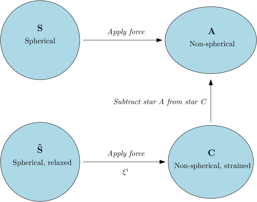
Figure 2: A schematic illustration showing the configurations in the force-based mountain scheme.

We can then consider the difference between stars A and C. By using (22) and (28), we obtain

$$\delta H_{i}^{\text{AC}}=\nabla^{j}t_{ij}(\xi).$$ (29)

We can note the similarity of (29) to (26). Indeed, comparing Figs. 1 and 2, we note the following. In Fig. 1, the addition of force $f_{i}$ maps star B to star A, generating a displacement $-\eta^{i}$, while in Fig. 2, the addition of the force $f_{i}$ maps star S̃ to star C, generating a displacement field $\xi^{i}$. It follows that, to a good approximation, these vector fields are related by

$$\eta^{i}=-\xi^{i}.$$ (30)

Comparing (29) to (26) then gives the corresponding relation between the associated scalar perturbations,

$$\delta H_{i}^{\text{SB}}=-\delta H_{i}^{\text{AC}}.$$ (31)

These relations are not exact, as in Fig. 1 the force $f_{i}$ acts upon star B, while in Fig. 2 it acts upon star S̃, but these two stars themselves differ from one another only in a perturbative way, so the difference in the action of $f_{i}$ on the two must be of second order.

This immediately suggests a strategy for computing the deformation of star B (i.e., $\delta H_{i}^{\text{SB}}$ and other perturbed quantities). We can easily compute the perturbations linking S and A (i.e., $\delta H_{i}^{\text{SA}}$ etc.), as this is just the perturbation of a spherical fluid star by the force $f_{i}$. We can, with only a little more effort, compute the perturbations linking star S̃ and C (i.e., $\delta H_{i}^{\text{SC}}$ etc.), as this is just the perturbation of a spherical elastic star by $f_{i}$. Then, we can take the difference between these two configurations to give the difference between star A and C (i.e., $\delta H_{i}^{\text{AC}}$ etc.), which is, up to an overall sign, the deformation of star B relative to star S that we require, as per (31).

As we are interested in computing maximum mountains, we will choose the force $f_{i}$ such that the breaking strain is reached at some point in the crust of star C. Note, however, that in this force-based approach, we will not be able to follow Ushomirsky et al. (2000) and find the solution where the strain is reached at all points (simultaneously) in the crust. This is a price one pays in adopting the force-based approach. We have, however, reduced the calculation of the mountain to two simpler calculations, both taking place on a spherical background and with readily implementable boundary conditions. We now go on to consider these calculations in detail.

4 Perturbation formalism

In order to develop the second strategy in detail, we take the background star to be non-rotating and the perturbations to be static. Our star is separated into three layers: a fluid core, an elastic crust and a fluid ocean. We choose to include a fluid layer outside the crust since at low densities the crustal lattice begins to melt and it also simplifies the matching to the exterior gravitational potential (Gittins, Andersson & Pereira, 2020). The crust only comes into the structure equations at the perturbative level.

From equations (3), (4) and (6), we obtain the Newtonian equations of structure for a non-rotating, fluid star,

$$m^{\prime}=4\uppi r^{2}\rho,$$ (32a)

$$p^{\prime}=-\rho\Phi^{\prime}$$ (32b)

and

$$\Phi^{\prime}=\frac{Gm}{r^{2}},$$ (32c)

where $m(r)$ is the mass enclosed in radius $r$. These equations are closed by supplying an equation of state (5).

4.1 Fluid perturbations

In order to calculate the relaxed configuration (star A), we need to introduce the force $f_{i}$. For practical purposes, it is convenient to write the force as the gradient of a potential, $\chi$,

$$f_{i}=-\rho\nabla_{i}\chi.$$ (33)

This is not the most general expression for the force but it allows us to combine $\chi$ with the gravitational potential, which simplifies the analysis. To make the notation more compact, we introduce the total perturbed potential, $U=\delta\Phi+\chi$.

At this point, we note that this is where our calculation differs from previous work (Ushomirsky et al., 2000; Haskell et al., 2006; Johnson-McDaniel & Owen, 2013). Previous calculations set out to evaluate the perturbed Euler equation (26) where the strain is taken with respect to the relaxed shape the crust wants to have (see Fig. 1). In our method, we start with the deforming force and evaluate (29), using the subtraction scheme (taking the difference between stars C and A) set out in Section 3. The use of this force is a subtle, but important, detail since without it one does not have the necessary freedom to impose all the boundary conditions of the problem. We emphasise this point since this issue was somewhat confused in the analysis of Haskell et al. (2006) who calculate perturbations of a spherical star but do not explicitly consider the force which sources them. It is for this reason that they were unable to satisfy the boundary condition on the potential at the surface. This point is elucidated below.

Recall that, as we discussed earlier, we assume all perturbed quantities to be expanded in spherical harmonics, but it will be sufficient for our discussion to focus on the $(l,m)=(2,2)$ mode. The system of equations which describes fluid perturbations then simplifies to a single second-order differential equation for the perturbed potential. From the perturbed Poisson’s equation (11), we get

$$\delta\Phi^{\prime\prime}+\frac{2}{r}\delta\Phi^{\prime}-\frac{\beta^{2}}{r^{2}}\delta\Phi=4\uppi G\delta\rho,$$ (34a)

where $$\beta\equiv\sqrt{l(l+1)}$$. The perturbed Euler equation (12) returns

$$\delta\rho=-\frac{\rho}{c_{\text{s}}^{2}}U.$$ (34b)

Therefore, provided a description of the perturbing force, equations (34) give a second-order equation that describes the perturbations in the fluid.

The perturbed potential must satisfy two boundary conditions. At the centre of the star the solution must be regular and at the surface it must match to the external solution. Therefore, in addition to $\chi$ being regular at the centre of the star and continuous at all interfaces, we must have

$$\delta\Phi(0)=0$$ (35a)

and

$$R\delta\Phi^{\prime}(R)=-(l+1)\delta\Phi(R).$$ (35b)

From regularity, we obtain an initial condition by expanding (34) in small $r$,

$$\delta\Phi(r)=a_{0}r^{l}[1+\mathcal{O}(r^{2})],$$ (36)

where $a_{0}$ is a constant which parametrises the amplitude of the perturbations. In the case when $\chi=0$ and there is no driving force, this initial condition provides sufficient information to calculate the perturbations up to the surface. At the surface, however, there is no freedom left to impose the surface boundary condition (35b) – except in the special case of $a_{0}=0$ where there are no perturbations. [This is the issue that the formalism of Haskell et al. (2006) suffers from, and why in that analysis a surface force had to be effectively introduced via a boundary condition.] This serves as a simple demonstration of the fact that an unforced, fluid equilibrium is a spherical star. Equations (34) with the boundary conditions (35) provide the necessary information to calculate perturbations in the fluid regions of the star sourced by a perturbing force.

4.2 The crust

In order to calculate the strained star (star C) in our scheme outlined in Section 3 (Fig. 2), we must consider the role of the elastic crust. We reiterate that we consider perturbations with respect to a spherical, reference star.

The elastic material is characterised by the shear-stress tensor,

$$t_{ij}=\mu\left(\nabla_{i}\xi_{j}+\nabla_{j}\xi_{i}-\frac{2}{3}g_{ij}\nabla_{k}\xi^{k}\right),$$ (37)

where $\mu$ is the shear modulus of the crust and $g_{ij}$ is the flat three-metric. Note that we also have

$$t_{ij}=2\mu\sigma_{ij},$$ (38)

where $\sigma_{ij}$ is the stress tensor. [This is a factor of two different to the expressions in Ushomirsky et al. (2000) and Haskell et al. (2006) but the same as used in Johnson-McDaniel & Owen (2013).] We use the static displacement vector appropriate for polar perturbations (Ushomirsky et al., 2000),

$$\xi^{i}=\xi_{r}(r)\nabla^{i}rY_{lm}+\frac{r}{\beta}\xi_{\perp}(r)\nabla^{i}Y_{lm}.$$ (39)

To make the application of the boundary conditions straightforward, we consider the perturbed traction vector, which may be identified from the perturbed Euler equation (13),

$$\begin{split}T^{i}&=(\delta pg^{ij}-t^{ij})\nabla_{j}r\\ &=[\delta p(r)-T_{1}(r)]\nabla^{i}rY_{lm}-rT_{2}(r)\nabla^{i}Y_{lm},\end{split}$$ (40)

where we have defined the following two variables related to the radial and tangential components of the traction:

$$T_{1}(r)Y_{lm}\equiv t_{rr}=\frac{2\mu}{3r}(-2\xi_{r}+\beta\xi_{\perp}+2r\xi_{r}^{\prime})Y_{lm}$$ (41a)

and

$$T_{2}(r)\nabla_{\theta}Y_{lm}\equiv\frac{t_{r\theta}}{r}=\frac{\mu}{\beta r}(\beta\xi_{r}-\xi_{\perp}+r\xi_{\perp}^{\prime})\nabla_{\theta}Y_{lm}.$$ (41b)

From the perturbed continuity equation (8), we then obtain

$$\begin{split}\delta\rho&=-\rho\xi_{r}^{\prime}-\left(\frac{2\rho}{r}+\rho^{\prime}\right)\xi_{r}+\frac{\beta\rho}{r}\xi_{\perp}\\ &=-\left(\frac{3\rho}{r}+\rho^{\prime}\right)\xi_{r}+\frac{3\beta\rho}{2r}\xi_{\perp}-\frac{3\rho}{4\mu}T_{1}.\end{split}$$ (42)

From the definitions of the traction variables (41), we have the following differential equations which describe the displacement vector:

$$\xi_{r}^{\prime}=\frac{1}{r}\xi_{r}-\frac{\beta}{2r}\xi_{\perp}+\frac{3}{4\mu}T_{1}$$ (43a)

and

$$\xi_{\perp}^{\prime}=-\frac{\beta}{r}\xi_{r}+\frac{1}{r}\xi_{\perp}+\frac{\beta}{\mu}T_{2}.$$ (43b)

From the radial part of the perturbed Euler equation (13) combined with the perturbed continuity equation (42),

$$\begin{split}\bigg{(}1+&\frac{3c_{\text{s}}^{2}\rho}{4\mu}\bigg{)}T_{1}^{\prime}=\rho U^{\prime}\\ -&\left[(c_{\text{s}}^{2})^{\prime}(3\rho+r\rho^{\prime})+c_{\text{s}}^{2}\left(\frac{3\beta^{2}\rho}{2r}+\rho^{\prime}-\frac{r\rho^{\prime 2}}{\rho}+r\rho^{\prime\prime}\right)\right]\frac{1}{r}\xi_{r}\\ +&\left[(c_{\text{s}}^{2})^{\prime}3\rho+c_{\text{s}}^{2}\left(\frac{3\rho}{r}+\rho^{\prime}\right)\right]\frac{\beta}{2r}\xi_{\perp}\\ -&\left[\frac{3}{r}+(c_{\text{s}}^{2})^{\prime}\frac{3\rho}{4\mu}+c_{\text{s}}^{2}\left(\frac{3\rho}{r}-\frac{\rho\mu^{\prime}}{\mu}+\rho^{\prime}\right)\frac{3}{4\mu}\right]T_{1}\\ +&\left(1+\frac{3c_{\text{s}}^{2}\rho}{2\mu}\right)\frac{\beta^{2}}{r}T_{2}.\end{split}$$ (43c)

Then, from the tangential piece of (13) we find

$$\begin{split}T_{2}^{\prime}=\frac{\rho}{r}U-&c_{\text{s}}^{2}(3\rho+r\rho^{\prime})\frac{1}{r^{2}}\xi_{r}\\ +&\left[\frac{3c_{\text{s}}^{2}\rho}{2}+\left(1-\frac{2}{\beta^{2}}\right)\mu\right]\frac{\beta}{r^{2}}\xi_{\perp}\\ +&\left(\frac{1}{2}-\frac{3c_{\text{s}}^{2}\rho}{4\mu}\right)\frac{1}{r}T_{1}-\frac{3}{r}T_{2}.\end{split}$$ (43d)

We also have the perturbed Poisson’s equation (34a), which combines with the perturbed continuity equation (42) to give

$$\begin{split}\delta\Phi^{\prime\prime}+\frac{2}{r}\delta\Phi^{\prime}-\frac{\beta^{2}}{r^{2}}\delta\Phi=-&4\uppi G\left(\frac{3\rho}{r}+\rho^{\prime}\right)\xi_{r}\\ +&6\uppi G\frac{\beta\rho}{r}\xi_{\perp}-3\uppi G\frac{\rho}{\mu}T_{1}.\end{split}$$ (43e)

Equations (43) form a coupled system of ordinary differential equations to describe the perturbations in the elastic material. We have compared our perturbation equations with that of Haskell et al. (2006) (in the limit of $\chi=0$) and noted several discrepancies. We find that these mistakes increase the maximum quadrupole estimates of Haskell et al. (2006) by three orders of magnitude.

4.3 Interface conditions

At this point, we address the boundary conditions at the fluid-elastic interfaces since we wish to connect perturbations in the fluid core and ocean with the elastic crust. Provided the density is smooth (which we assume), the perturbed potential, $\delta\Phi$, and its derivative, $\delta\Phi^{\prime}$, must be continuous at an interface. To see how the other perturbed quantities behave at an interface, we must consider the perturbed traction (40).

This admits two quantities which must be continuous: the radial and tangential components. Since the shear modulus vanishes in the fluid, continuity of the radial traction, $(\delta p-T_{1})$, provides an algebraic relation which must hold true at an interface,

$$\begin{split}\rho U_{\text{F}}=&\left(1+\frac{3c_{\text{s}}^{2}\rho}{4\mu}\right)T_{1\text{E}}\\ &+c_{\text{s}}^{2}\left[\left(\frac{3\rho}{r}+\rho^{\prime}\right)\xi_{r\text{E}}-\frac{3\beta\rho}{2r}\xi_{\perp\text{E}}\right],\end{split}$$ (44)

where the subscripts F and E denote the fluid and elastic sides of the interface, respectively. We note that the radial displacement, $\xi_{r}$ must be continuous at a boundary, however, this does not necessarily have to be the case for the tangential piece, $\xi_{\perp}$. From the tangential part of the traction, we have $T_{2}=0$ at a fluid-elastic interface.

In reference to the maximally strained approach of Ushomirsky et al. (2000) and Johnson-McDaniel & Owen (2013), we note that, if one assumes the shear modulus smoothly goes to zero at a fluid-elastic interface, then the tangential traction condition is trivially satisfied [see (41b)]. This would effectively result in the displacement vector in the crust being arbitrary since there are not enough boundary conditions to constrain it. It is not clear how to resolve this issue.

In the fluid regions of the star, the perturbations are governed by equations (34) and so are described by the variables, $(\delta\Phi^{\prime},\delta\Phi)$. In the crust, we have a more complex structure with equations (43) and quantities, $(\delta\Phi^{\prime},\delta\Phi,\xi_{r},\xi_{\perp},T_{1},T_{2})$. We assume the force is known. The perturbations in the elastic crust present a boundary-value problem. For the six variables, we have six boundary conditions: continuity of $\delta\Phi^{\prime}$ and $\delta\Phi$ at the core-crust transition and the two traction conditions – (44) and $T_{2}=0$ – at both interfaces. Therefore, the problem is well posed.

Additionally, it is straightforward to show that the boundary condition on the Lagrangian variation of the pressure, $\Delta p(R)=0$, is trivially satisfied by the background structure.

5 The deforming force

The formalism we detail above requires a description of the deforming force which causes the star to have a non-spherical shape. Because of the abstract nature of this force, it is difficult to prescribe without a detailed evolutionary calculation of the history of the star. As a proof-of-principle calculation, we examine three example sources.

We use a polytropic equation of state,

$$p(\rho)=K\rho^{1+1/n},$$ (45)

where $K$ is a constant of proportionality and $n$ is the polytropic constant. We work with $n=1$ and generate background models with $M=$1.4\text{\,}\mathrm{\mbox{$M_{\odot}$}}$$, $R=$10\text{\,}\mathrm{km}$$. For the shear-modulus profile in the crust, we consider a simple linear model (Haskell et al., 2006),

$$\mu(\rho)=\kappa\rho,$$ (46)

where $\kappa=${10}^{16}\text{\,}{\mathrm{cm}}^{2}\text{\,}{\mathrm{s}}^{-2}$$. We assume the core-crust transition to occur at $\rho_{\text{base}}=$2\text{\times}{10}^{14}\text{\,}\mathrm{g}\text{\,}{\mathrm{cm}}^{-3}$$ [which is the same as Ushomirsky et al. (2000)], while the crust-ocean transition is at $\rho_{\text{top}}=${10}^{6}\text{\,}\mathrm{g}\text{\,}{\mathrm{cm}}^{-3}$$ (Gittins et al., 2020).

We consider three sources for the perturbations: (i) a potential which satisfies Laplace’s equation, (ii) a potential which satisfies Laplace’s equation but does not act in the core and (iii) a thermal pressure perturbation. For each prescription, we generate two stars – a relaxed star, which experiences purely fluid perturbations (star A in Fig. 2), and a strained star, which experiences elastic perturbations in the crust (star C in Fig. 2). We normalise the perturbations by ensuring the strained star reaches breaking strain at a point in the crust, subject to the von Mises criterion, and that the relaxed star experiences the same force. This allows us to work out the quadrupole moment of each star. Our results for the three sources are summarised in Table 1.

Table 1: The maximum quadrupoles and ellipticities from the different models. For each case, we show the quadrupole, $Q_{22}^{\text{relaxed}}$, and ellipticity, $\epsilon^{\text{relaxed}}$, for the relaxed star and the difference relative to the strained star with quadrupole $Q_{22}^{\text{strained}}$ and ellipticity $\epsilon^{\text{strained}}$.

Source	$|Q_{22}^{\text{relaxed}}|$ / $\mathrm{g}\text{\,}{\mathrm{cm}}^{2}$	$|\epsilon^{\text{relaxed}}|$	$|Q_{22}^{\text{strained}}-Q_{22}^{\text{relaxed}}|$ / $\mathrm{g}\text{\,}{\mathrm{cm}}^{2}$	$|\epsilon^{\text{strained}}-\epsilon^{\text{relaxed}}|$
Solution of Laplace’s equation	$2.4\text{\times}{10}^{43}$	$3.1\text{\times}{10}^{-2}$	$1.7\text{\times}{10}^{37}$	$2.2\text{\times}{10}^{-8}$
Solution of Laplace’s equation (outside core)	$1.4\text{\times}{10}^{41}$	$1.8\text{\times}{10}^{-4}$	$4.4\text{\times}{10}^{38}$	$5.7\text{\times}{10}^{-7}$
Thermal pressure perturbation	$9.2\text{\times}{10}^{38}$	$1.2\text{\times}{10}^{-6}$	$4.0\text{\times}{10}^{38}$	$5.2\text{\times}{10}^{-7}$

To solve the coupled sets of ordinary differential equations (34) and (43), we used an explicit fifth-order Runge-Kutta method implemented in the solve_ivp function from the scipy library. The structure in the fluid core may be straightforwardly calculated using equations (34) with boundary condition (35a). The crust presents a boundary-value problem with the interface conditions described in Section 4.3. There are a variety of numerical techniques to solve such problems. Due to the linearity of the system (43), we used the linearly independent scheme described in Appendix B of Gittins et al. (2020). With the perturbations in the crust, one can integrate equations (34) through the fluid ocean to the surface. At this point, one can verify that the boundary condition at the surface (35b) is automatically satisfied.

5.1 A solution of Laplace’s equation

The first example we consider is based on the form of the deforming potential for tidal deformations [see, e.g., Andersson & Pnigouras (2020)]. The source potential is taken to be a solution of Laplace’s equation,

$$\nabla^{2}\chi=0.$$ (47)

This example is particularly convenient since the perturbed Poisson’s equation (11) is simply modified by $\delta\Phi\rightarrow U$. Therefore, we may write

$$\nabla^{2}U=4\uppi G\delta\rho.$$ (48)

The total perturbed potential must be regular at the origin, $U(0)=0$.

By using the definition of the multipole moment (1) with the perturbed Poisson’s equation (34a), one can show through integration by parts,

$$Q_{lm}=-\frac{(2l+1)R^{l+1}}{4\uppi G}\delta\Phi(R),$$ (49)

where the boundary conditions (35) have been used for simplification. This result, perhaps more familiar in relativistic calculations, shows that one can obtain the multipole moments from the variations of the potential at the surface. One can also write the multipole in terms of the total perturbed potential,

$$Q_{lm}=\frac{R^{l+1}}{4\uppi G}[RU^{\prime}(R)-lU(R)].$$ (50)

The advantage of writing the multipole in this way is that one does not need to disentangle the two potentials ($\chi$ and $\delta\Phi$) from $U$.

The source potential must be regular at the centre and so it must be of the form,

$$\chi(r)=Ar^{l},$$ (51)

where $A$ is a constant. Its value will be chosen to ensure the star is maximally strained at some point in the crust. The source potential at the surface is given by

$$\chi(R)=\frac{1}{2l+1}[RU^{\prime}(R)+(l+1)U(R)].$$ (52)

It is this quantity that we use to ensure that the relaxed and strained stars experience the same force.

To make sure the star is maximally strained we calculate the von Mises strain, $\bar{\sigma}$. The von Mises strain is defined using the strain tensor,

$$\bar{\sigma}^{2}\equiv\frac{1}{2}\sigma_{ij}\sigma^{ij}.$$ (53)

The von Mises criterion states that an elastic material will reach its yield limit when $\bar{\sigma}\geq\bar{\sigma}_{\text{max}}$. For $(l,m)=(2,2)$ perturbations, we have

$$\begin{split}\bar{\sigma}^{2}=\frac{5}{256\uppi}\Bigg{\{}6\sin^{2}\theta\Bigg{[}3\sin^{2}\theta\cos^{2}2\phi&\left(\frac{T_{1}}{\mu}\right)^{2}\\ +4(3+\cos 2\theta-2\sin^{2}\theta\cos 4\phi)&\left(\frac{T_{2}}{\mu}\right)^{2}\Bigg{]}\\ +(35+28\cos 2\theta+\cos 4\theta+8\sin^{4}\theta\cos 4\phi)&\left(\frac{\xi_{\perp}}{r}\right)^{2}\Bigg{\}}.\end{split}$$ (54)

Since the von Mises strain is a function of position, we can identify where the strain is highest (and, thus, the crust will break first) and take that point to be at breaking strain, which we assume to be $\bar{\sigma}_{\text{max}}=10^{-1}$ (Horowitz & Kadau, 2009).

Thus, for the strained star (star C) we integrate equations (34) for the core and ocean and integrate equations (43) in the elastic crust. The relaxed star (star A) is generated using equations (34) for the entire star. The perturbations are normalised by ensuring that the point in the crust where the strain is highest reaches breaking strain, according to (54). The force associated with this deformation (52) is then taken to be the same for the relaxed star. Figs. 3 and 4 show the results for the strained star. In Fig. 3 we show how the perturbed traction is continuous at the fluid-elastic interfaces. We note that Fig. 4 shows how the dominant contribution to the von Mises strain comes from the radial traction component. This is also true for the other forces we consider. It is at the top of the crust that the star is the weakest in the $(l,m)=(2,2)$ mode. The quadrupoles are calculated using (50). The relaxed star attains a quadrupole of $|Q_{22}^{\text{relaxed}}|=$2.4\text{\times}{10}^{43}\text{\,}\mathrm{g}\text{\,}{\mathrm{cm}}^{2}$$, which corresponds to an ellipticity of $|\epsilon^{\text{relaxed}}|=$3.1\text{\times}{10}^{-2}$$. The difference between the strained and relaxed star is $|Q_{22}^{\text{strained}}-Q_{22}^{\text{relaxed}}|=$1.7\text{\times}{10}^{37}\text{\,}\mathrm{g}\text{\,}{\mathrm{cm}}^{2}$$, $|\epsilon^{\text{strained}}-\epsilon^{\text{relaxed}}|=$2.2\text{\times}{10}^{-8}$$.

The very different sizes of $|\epsilon^{\text{relaxed}}|$ and $|\epsilon^{\text{strained}}-\epsilon^{\text{relaxed}}|$ reported in Table 1 have a natural interpretation. The large ellipticity represented by $|\epsilon^{\text{relaxed}}|$ corresponds to a star whose deformation is supported by the external force $f_{i}$, with a size limited only by the crustal breaking strain. In this case, the (non-zero) shear modulus of the crust plays little role. [It is this sort of configuration that was effectively considered in Haskell et al. (2006), where in that case the force that was implicitly introduced was a force per unit area, applied at the surface.] In contrast, the ellipticity represented by $|\epsilon^{\text{strained}}-\epsilon^{\text{relaxed}}|$ is that supported by the shear strains of the crust when the external force is removed, and therefore is sensitive to the crust’s shear modulus. As is readily captured by simple back-of-the-envelope estimates, the relative sizes of these two ellipticities are related to the fact that the gravitational binding energy of the star is orders of magnitude larger than the Coulomb binding energy of the crustal lattice [see, e.g., Jones (2002)].

We observe that the ellipticity $|\epsilon^{\text{strained}}-\epsilon^{\text{relaxed}}|=$2.2\text{\times}{10}^{-8}$$ is notably smaller than what has been found in previous work [equations (14)–(16)]. This is not surprising, as these previous studies considered strain fields that were maximal everywhere, as opposed to at a single point. With a view to producing larger ellipticities, we will therefore consider some different choices of external force field.

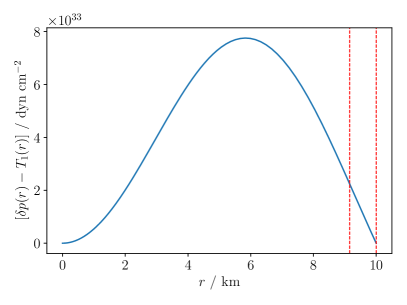
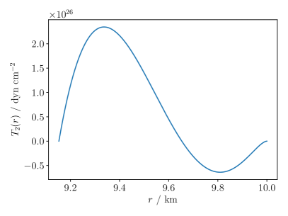
Figure 3: The radial (left panel) and tangential (right panel) components of the perturbed traction as functions of radius for the potential solution to Laplace’s equation. The vertical red dashed lines in the left panel indicate the base and the top of the crust. Regarding the horizontal range in the right panel, recall that $T_{2}$ only has a finite value in the crust.

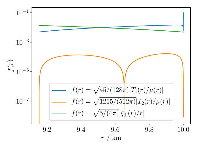
Figure 4: The strain components in (54) maximised over $(\theta,\phi)$ against radius for the potential solution to Laplace’s equation.

5.2 A solution of Laplace’s equation outside the core

We consider a special case of the above source: a source potential that does not act in the core – instead, it only manifests itself in the crust and ocean. The motivation for considering this special case is regularity at the centre will not be a necessary condition on the source potential since it does not exist at the origin. Also, we note that Haskell et al. (2006) found that a similar example produced their largest quadrupole moment. We then have the general solution to Laplace’s equation (47),

$$\chi(r)=Ar^{l}+B/r^{l+1},$$ (55)

where $B$ is another constant. This expression is taken to be true for the base of the crust and above.

As this model is somewhat artificial, we have to make a number of assumptions with regards to its prescription. We take the core to be unperturbed and have $\delta\Phi=\xi_{r}=0$ in the core. With the introduction of the source potential in the crust, there will be a discontinuity in $U$ at the core-crust interface. However, we insist that $\delta\Phi$ must be continuous. This discontinuity is relevant for the radial traction condition (44) where $U_{\text{F}}=0$, but has a finite value in the crust due to the source potential.

The quadrupole may be calculated from (49). The matching with the total perturbed potential needs to be adjusted to take into account the additional $1/r^{l+1}$ term from the external field. Therefore, we have

$$Q_{lm}=\frac{R^{l+1}}{4\uppi G}[RU^{\prime}(R)-lU(R)]+\frac{2l+1}{4\uppi G}B.$$ (56)

As in the previous case, we generate a relaxed star and a maximally strained star. One must vary either $A$ or $B$ to ensure the surface boundary condition (35b) is satisfied. We normalise the relaxed star so that it experiences the same source potential (55). The results for this case are shown in Figs. 5 and 6. As in the above example, the $T_{1}$ component dominates the von Mises strain and the crust breaks at the top. We find $|Q_{22}^{\text{relaxed}}|=$1.4\text{\times}{10}^{41}\text{\,}\mathrm{g}\text{\,}{\mathrm{cm}}^{2}$$, $|\epsilon^{\text{relaxed}}|=$1.8\text{\times}{10}^{-4}$$ and $|Q_{22}^{\text{strained}}-Q_{22}^{\text{relaxed}}|=$4.4\text{\times}{10}^{38}\text{\,}\mathrm{g}\text{\,}{\mathrm{cm}}^{2}$$, $|\epsilon^{\text{strained}}-\epsilon^{\text{relaxed}}|=$5.7\text{\times}{10}^{-7}$$.

Compared to the previous result, the quadrupole difference between the relaxed and strained stars has increased by an order of magnitude. This is within a factor of a few of previous maximum-mountain calculations, and illustrates the dependence on the force prescription.

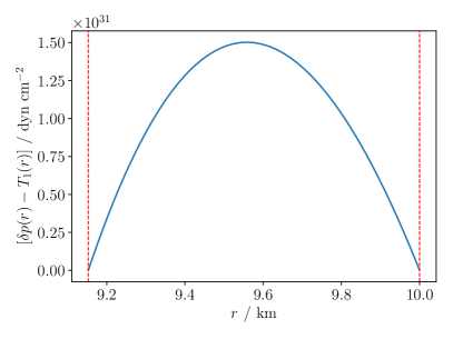
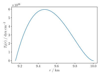
Figure 5: The radial (left panel) and tangential (right panel) components of the perturbed traction as functions of radius for the potential solution to Laplace’s equation outside the core. The vertical red dashed lines in the left panel indicate the base and the top of the crust. Regarding the horizontal range in the right panel, recall that $T_{2}$ only has a finite value in the crust.

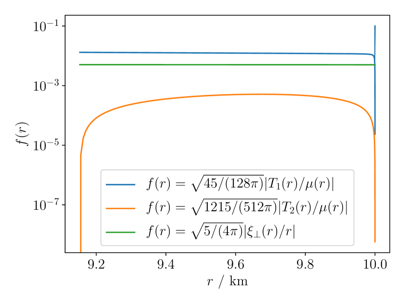
Figure 6: The strain components in (54) maximised over $(\theta,\phi)$ against radius for the potential solution to Laplace’s equation outside the core.

5.3 A thermal pressure perturbation

The third source for the perturbations we examine is motivated by a thermal pressure perturbation. Note that the approach we use for this example could be applied more generally to consider non-barotropic matter where the pressure is adjusted, relative to the barotropic case, at the perturbative level. We assume the thermal pressure to be of the ideal-gas form,

$$\delta p_{\text{th}}=\frac{k_{\text{B}}\rho}{m_{\text{u}}}\delta T,$$ (57)

where $k_{\text{B}}$ is the Boltzmann constant, $m_{\text{u}}$ is the atomic mass unit and $\delta T$ is the temperature perturbation. To interpret this thermal pressure as a force, we identify

$$\rho\nabla_{i}\chi=\nabla_{i}\delta p_{\text{th}}=\frac{k_{\text{B}}}{m_{\text{u}}}\nabla_{i}(\rho\delta T).$$ (58)

The temperature perturbation must be regular at the origin. For simplicity we assume it to be quadratic,

$$\delta T(r)=\left(\frac{r}{R}\right)^{2}\delta T(R),$$ (59)

where $\delta T(R)$ corresponds to the perturbation of the temperature at the surface. Both the relaxed and strained configurations experience the same temperature perturbation. We show the results in Figs. 7 and 8. We now find the crust breaks when $\delta T(R)=$3.5\text{\times}{10}^{6}\text{\,}\mathrm{K}$$. We obtain the results $|Q_{22}^{\text{relaxed}}|=$9.2\text{\times}{10}^{38}\text{\,}\mathrm{g}\text{\,}{\mathrm{cm}}^{2}$$, $|\epsilon^{\text{relaxed}}|=$1.2\text{\times}{10}^{-6}$$ and $|Q_{22}^{\text{strained}}-Q_{22}^{\text{relaxed}}|=$4.0\text{\times}{10}^{38}\text{\,}\mathrm{g}\text{\,}{\mathrm{cm}}^{2}$$, $|\epsilon^{\text{strained}}-\epsilon^{\text{relaxed}}|=$5.2\text{\times}{10}^{-7}$$. This result is of the same order of magnitude to the potential outside the core.

It is interesting to note that while the values of the ellipticities $|\epsilon^{\text{strained}}|$ and $|\epsilon^{\text{relaxed}}|$ vary by about four orders of magnitude for the three deforming forces we consider, the variation in the actual ellipticity of the mountain, $|\epsilon^{\text{strained}}-\epsilon^{\text{relaxed}}|$, is relatively modest, about one order of magnitude (see Table 1). This is presumably a reflection of the fact that in all three cases we consider the same star with the same crustal breaking strain and shear modulus, so all stars have a similar ability to support deformations.

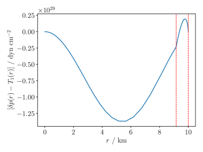
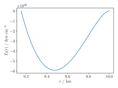
Figure 7: The radial (left panel) and tangential (right panel) components of the perturbed traction as functions of radius for the temperature perturbation. The vertical red dashed lines in the left panel indicate the base and the top of the crust. Regarding the horizontal range in the right panel, recall that $T_{2}$ only has a finite value in the crust.

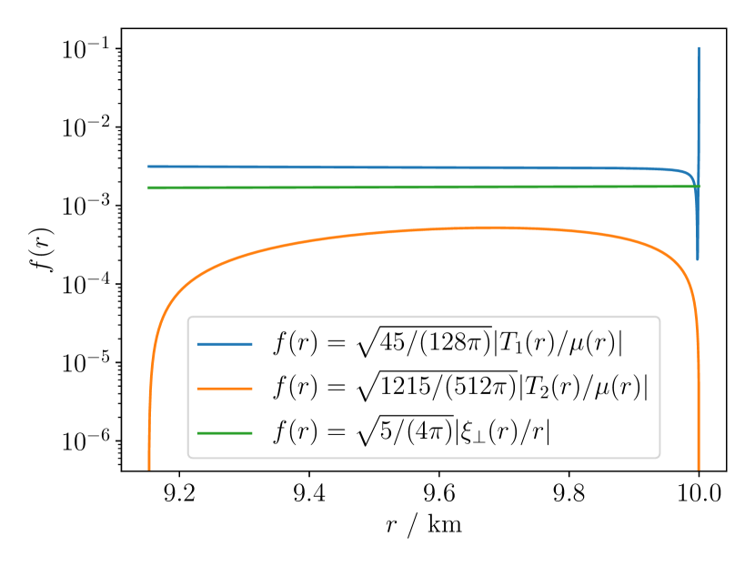
Figure 8: The strain components in (54) maximised over $(\theta,\phi)$ against radius for the temperature perturbation.

6 Conclusions

The question of the maximum mountain a neutron star crust can support is an interesting problem. Such an estimate provides upper limits on the strength of gravitational-wave emission from rotating neutron stars, as well as having implications for the maximum spin-frequency limit that these systems can attain.

We returned to this problem to tackle some of the pertinent assumptions made in previous work. We have discussed how previous estimates have not dealt appropriately with boundary conditions that must be satisfied for realistic neutron star models. The calculations of Ushomirsky et al. (2000) and Johnson-McDaniel & Owen (2013) both assumed a specific form for the strain that takes the star away from its relaxed shape and ensures the crust is maximally strained at every point. However, such a strain is somewhat unphysical since it does not respect the continuity of the traction vector. Additionally, the approach of Haskell et al. (2006), while satisfying the traction conditions at the crust-core boundary, did not obey the boundary condition on the potential at the surface. This was due to the calculation assuming the relaxed configuration is spherical and implicitly using a surface force to deform the star. There were also errors present in the perturbation equations of Haskell et al. (2006) which change their results by several orders of magnitude.

An important simplification of the previous studies was to not explicitly calculate the non-spherical, relaxed shape that the strain is taken with respect to. As we have shown, such a description requires the introduction of a perturbing force which takes the star away from sphericity. We found such a discussion was missing in prior studies and, hence, have provided a demonstration that shows, provided one has a description of the strain, how the relaxed shape can calculated.

We found that including this force is crucial in enabling one to satisfy all the boundary conditions. Therefore, we have introduced a novel scheme for calculating the maximum quadrupole deformation that a neutron star can sustain and have demonstrated how our scheme is entirely equivalent to the approach of preceding calculations. Crucially, the formalism satisfies all the boundary conditions of the problem. One of the key advantages of our approach is that one computes all relevant quantities, including the shape of the relaxed star. However, one must provide a prescription for the deforming force.

There is obviously significant freedom in what one may choose for the form of this force and, indeed, the formalism we have presented can be used for any deforming force that has the form (33). Furthermore, it would not be difficult to adjust this formalism for other forces. However, evolutionary calculations will be necessary to fully motivate the form of the force. Thus, we surveyed three simple examples for the source of the mountains. We obtained the largest quadrupole for the (somewhat artificial) case where the perturbing potential is a solution to Laplace’s equation, but leaves the core unperturbed. All of our results are between a factor of a few to two orders of magnitude below that of prior estimates for the maximum mountain a neutron star may support. That our results were smaller is not surprising, as our maximum mountains were constructed so that the breaking strain was reached at only a single point. An immediate question would be if there is a reasonable scenario that bridges the gap between relaxed configurations associated with a specific force and configurations following from specifying the strain. It seems inevitable that the answer will rely on evolutionary scenarios, leading to mountain formation, a problem that has not yet attracted the attention it deserves.

An example of a promising scenario through which a rotating neutron star may radiate gravitational waves is accretion from a binary companion. As the gas is accreted onto the surface of the star, chemical reactions take place which change the composition. Such changes in the composition can, in turn, result in the star attaining a non-trivial quadrupole moment (Bildsten, 1998; Ushomirsky et al., 2000). Additionally, there has been some effort towards calculating mountains on accreting neutron stars that are sustained by the magnetic field (Melatos & Payne, 2005; Payne & Melatos, 2006; Priymak et al., 2011). We note that, in our calculation, we only consider barotropic matter. This is appropriate to describe equilibrium stellar models. Indeed, if the star is in equilibrium, accreted and non-accreted matter may be described using barotropic equations of state (Haskell et al., 2006). However, for evolutionary calculations, like those described above, one may need to consider non-barotropic features and, as we noted in Section 5.3, the formalism we have presented could be used with such aspects at the perturbative level.

As an (admittedly phenomenological) indication of a possible solution, it may be worth pointing out that our approach to elasticity is somewhat simplistic. We have followed the usual assumption that the crust can be well described as an elastic solid (represented by a linear stress-strain relation) until it reaches the breaking strain, at which point the crust fails and all the strain is released. This model accords well with the molecular dynamics simulations of Horowitz & Kadau (2009), but it is worth noting that laboratory materials tends to behave slightly differently (Ottosen & Ristinmaa, 2005). In particular, one typically finds that material deforms plastically for some level of strain before the ultimate failure. This introduces the yield strain as the point above which the stress-strain relationship is no longer linear and raises (difficult) questions regarding the plastic behaviour (the matter may harden, allowing stresses to continue building, or soften, leading to reduced stress as the strain increases). State-of-the-art simulations suggest a narrow region of plastic behaviour before the crust fails (Horowitz & Kadau, 2009), but one should perhaps keep in mind that the levels of shear involved in the simulation may not lead to a true representation of matter that is deformed more gently. Let us, for the sake of the argument, suppose that this is the case and that the crust exhibits ideal plasticity above then chosen yield strain. If this were to happen, the strain would locally saturate at the yield limit even if the imposed force increased. One can then imagine applying a deforming force to source a neutron star mountain and then increasing it until some point in the crust reaches yield strain. This is essentially the calculation we have done, as we did not model the behaviour beyond this point. Allowing for (ideal) plastic flow as the force is further increased, one may envisage that the entire crust may saturate at the yield strain. This is, of course, pure speculation [although there have been several notable discussions about the relevance of plastic deformations of the neutron star crust; see Smoluchowski & Welch (1970), Jones (2003) and Chugunov & Horowitz (2010)], but it might explain how a real system could reach the maximum strain configuration imposed in the Ushomirsky et al. (2000) argument. As we already suggested, detailed evolutionary calculations which take into account the physical processes that produce the mountain will be required to make progress on the problem.

Another natural avenue for future research is to generalise our calculation to relativity. This should be reasonably straightforward to do. One would need to use the relativistic equivalents of the perturbation equations [see, e.g., Gittins et al. (2020)]. This would be an important step as it brings realistic equations of state into play.

Data availability

Additional data underlying this article will be shared on reasonable request to the corresponding author.

Appendix A Calculating the relaxed shape

In this appendix, we demonstrate that the relaxed configuration that is implied, but not calculated, in maximum-mountain calculations Ushomirsky et al. (2000) and Johnson-McDaniel & Owen (2013) is calculable.

Suppose one knows the strain of star B, $\sigma_{ij}(\eta)$ (see Fig. 1; Section 3). [This is the case in Ushomirsky et al. (2000) and Johnson-McDaniel & Owen (2013).] From the strain tensor it is possible to obtain the displacement vector, $\eta^{i}$, which sources the strain.

We note the following relations: $\delta\rho$ and $\delta p$ are related through the equation of state (10), the perturbed Poisson’s equation (11) couples $\delta\rho$ and $\delta\Phi$ and (20) links $\delta\rho$, $\delta p$, $\delta\Phi$ and $\delta H_{i}$. Therefore, it follows that if any one of $(\delta\rho,\delta p,\delta\Phi,\delta H_{i})$ are known, the other quantities can, in principle, be calculated.

We begin with (26). Since we know the strain tensor that takes one from star A to star B, we also know $\delta H_{i}^{\text{SB}}$. This means we have $(\delta\rho_{\text{SB}},\delta p_{\text{SB}},\delta\Phi_{\text{SB}})$. It is this logic, that enables Ushomirsky et al. (2000) and Johnson-McDaniel & Owen (2013) to compute the quadrupole moment from just the strain tensor.

By considering variations between star A (22) and star B (24), we find

$$\delta H_{i}^{\text{AB}}=-f_{i}+\nabla^{j}t_{ij}(\eta).$$ (60)

We know $t_{ij}(\eta)$, but not $f_{i}$ or $\delta H_{i}^{\text{AB}}$. However, we can obtain $\delta H_{i}^{\text{AB}}$. The quantity, $\delta H_{i}^{\text{AB}}$, is generated by the change in shape from star A to star B. This is described by the displacement, $\eta^{i}$. In particular, the two density fields, $\rho_{\text{A}}$ and $\rho_{\text{B}}$, are linked through the perturbed continuity equation (8). It, therefore, follows that

$$\delta H_{i}^{\text{AB}}=\delta H_{i}^{\text{AB}}(\eta).$$ (61)

We rearrange (60) to obtain an expression for the force,

$$f_{i}=-\delta H_{i}^{\text{AB}}(\eta)+\nabla^{j}t_{ij}(\eta).$$ (62)

Provided $\eta^{i}$, we can calculate the force which takes the star from a spherical shape (star S) to the relaxed shape (star A).

Using (21) and (22), we have

$$\delta H_{i}^{\text{SA}}=f_{i}.$$ (63)

This determines $\delta H_{i}^{\text{SA}}$ and, therefore, also $(\delta\rho_{\text{SA}},\delta p_{\text{SA}},\delta\Phi_{\text{SA}})$. This means one can obtain the shape of the relaxed star, supported by a force, $f_{i}$, with the property that when the force is removed the star obtains a strained configuration, according to the displacement vector, $\eta^{i}$.

References

- Aasi et al. (2013) Aasi J., et al., 2013, Phys. Rev. D, 87, 042001
- Aasi et al. (2014) Aasi J., et al., 2014, ApJ, 785, 119
- Aasi et al. (2015a) Aasi J., et al., 2015a, Phys. Rev. D, 91, 022004
- Aasi et al. (2015b) Aasi J., et al., 2015b, Phys. Rev. D, 91, 062008
- Abadie et al. (2010) Abadie J., et al., 2010, Class. Quantum Gravity, 27, 173001
- Abadie et al. (2011a) Abadie J., et al., 2011a, Phys. Rev. D, 83, 042001
- Abadie et al. (2011b) Abadie J., et al., 2011b, ApJ, 737, 93
- Abadie et al. (2012) Abadie J., et al., 2012, Phys. Rev. D, 85, 022001
- Abbott et al. (2004) Abbott B., et al., 2004, Phys. Rev. D, 69, 082004
- Abbott et al. (2005a) Abbott B., et al., 2005a, Phys. Rev. D, 72, 102004
- Abbott et al. (2005b) Abbott B., et al., 2005b, Phys. Rev. Lett., 94, 181103
- Abbott et al. (2007a) Abbott B., et al., 2007a, Phys. Rev. D, 76, 042001
- Abbott et al. (2007b) Abbott B., et al., 2007b, Phys. Rev. D, 76, 082001
- Abbott et al. (2008a) Abbott B., et al., 2008a, Phys. Rev. D, 77, 022001
- Abbott et al. (2008b) Abbott B., et al., 2008b, ApJ, 683, L45
- Abbott et al. (2009) Abbott B., et al., 2009, Phys. Rev. D, 79, 022001
- Abbott et al. (2010) Abbott B. P., et al., 2010, ApJ, 713, 671
- Abbott et al. (2016) Abbott B. P., et al., 2016, Phys. Rev. D, 94, 042002
- Abbott et al. (2017a) Abbott B. P., et al., 2017a, Phys. Rev. D, 95, 122003
- Abbott et al. (2017b) Abbott B. P., et al., 2017b, Phys. Rev. D, 96, 062002
- Abbott et al. (2017c) Abbott B. P., et al., 2017c, Phys. Rev. D, 96, 122006
- Abbott et al. (2017d) Abbott B. P., et al., 2017d, Phys. Rev. Lett., 119, 161101
- Abbott et al. (2017e) Abbott B. P., et al., 2017e, ApJ, 839, 12
- Abbott et al. (2017f) Abbott B. P., et al., 2017f, ApJ, 847, 47
- Abbott et al. (2018a) Abbott B. P., et al., 2018a, Phys. Rev. D, 97, 102003
- Abbott et al. (2018b) Abbott B. P., et al., 2018b, Phys. Rev. Lett., 120, 031104
- Abbott et al. (2019a) Abbott B. P., et al., 2019a, Phys. Rev. D, 99, 122002
- Abbott et al. (2019b) Abbott B. P., et al., 2019b, Phys. Rev. D, 100, 122002
- Abbott et al. (2019c) Abbott B. P., et al., 2019c, Phys. Rev. D, 100, 024004
- Abbott et al. (2019d) Abbott B. P., et al., 2019d, ApJ, 875, 122
- Abbott et al. (2019e) Abbott B. P., et al., 2019e, ApJ, 879, 10
- Abbott et al. (2020a) Abbott R., et al., 2020a, preprint, (arXiv:2007.14251)
- Abbott et al. (2020b) Abbott B. P., et al., 2020b, ApJ, 892, L3
- Andersson (1998) Andersson N., 1998, ApJ, 502, 708
- Andersson & Pnigouras (2020) Andersson N., Pnigouras P., 2020, Phys. Rev. D, 101, 083001
- Andersson et al. (1999) Andersson N., Kokkotas K. D., Stergioulas N., 1999, ApJ, 516, 307
- Baym & Pines (1971) Baym G., Pines D., 1971, Ann. Phys., 66, 816
- Bildsten (1998) Bildsten L., 1998, ApJ, 501, L89
- Chugunov & Horowitz (2010) Chugunov A. I., Horowitz C. J., 2010, MNRAS, 407, L54
- Cook et al. (1994) Cook G. B., Shapiro S. L., Teukolsky S. A., 1994, ApJ, 424, 823
- Douchin & Haensel (2001) Douchin F., Haensel P., 2001, A&A, 380, 151
- Friedman & Schutz (1978) Friedman J. L., Schutz B. F., 1978, ApJ, 221, 937
- Gittins & Andersson (2019) Gittins F., Andersson N., 2019, MNRAS, 488, 99
- Gittins et al. (2020) Gittins F., Andersson N., Pereira J. P., 2020, Phys. Rev. D, 101, 103025
- Haskell et al. (2006) Haskell B., Jones D. I., Andersson N., 2006, MNRAS, 373, 1423
- Hessels et al. (2006) Hessels J. W. T., Ransom S. M., Stairs I. H., Freire P. C. C., Kaspi V. M., Camilo F., 2006, Science, 311, 1901
- Horowitz & Kadau (2009) Horowitz C. J., Kadau K., 2009, Phys. Rev. Lett., 102, 191102
- Johnson-McDaniel & Owen (2013) Johnson-McDaniel N. K., Owen B. J., 2013, Phys. Rev. D, 88, 044004
- Jones (2002) Jones D. I., 2002, Class. Quantum Gravity, 19, 1255
- Jones (2003) Jones P. B., 2003, ApJ, 595, 342
- Keer & Jones (2015) Keer L., Jones D. I., 2015, MNRAS, 446, 865
- Lattimer & Prakash (2007) Lattimer J. M., Prakash M., 2007, Phys. Rep., 442, 109
- Melatos & Payne (2005) Melatos A., Payne D. J. B., 2005, ApJ, 623, 1044
- Osborne & Jones (2020) Osborne E. L., Jones D. I., 2020, MNRAS, 494, 2839
- Ottosen & Ristinmaa (2005) Ottosen N. S., Ristinmaa M., 2005, The Mechanics of Constitutive Modeling. Elsevier, United States, doi:10.1016/B978-0-08-044606-6.X5000-0
- Owen (2005) Owen B. J., 2005, Phys. Rev. Lett., 95, 211101
- Papaloizou & Pringle (1978) Papaloizou J., Pringle J. E., 1978, MNRAS, 184, 501
- Payne & Melatos (2006) Payne D. J. B., Melatos A., 2006, ApJ, 641, 471
- Priymak et al. (2011) Priymak M., Melatos A., Payne D. J. B., 2011, MNRAS, 417, 2696
- Singh et al. (2020) Singh N., Haskell B., Mukherjee D., Bulik T., 2020, MNRAS, 493, 3866
- Smoluchowski & Welch (1970) Smoluchowski R., Welch D. O., 1970, Phys. Rev. Lett., 24, 1191
- Ushomirsky et al. (2000) Ushomirsky G., Cutler C., Bildsten L., 2000, MNRAS, 319, 902
- Wagoner (1984) Wagoner R. V., 1984, ApJ, 278, 345