Inductively Representing Out-of-Knowledge-Graph Entities by
Optimal Estimation Under Translational Assumptions

Abstract

Conventional Knowledge Graph Completion (KGC) assumes that all test entities appear during training. However, in real-world scenarios, Knowledge Graphs (KG) evolve fast with out-of-knowledge-graph (OOKG) entities added frequently, and we need to represent these entities efficiently. Most existing Knowledge Graph Embedding (KGE) methods cannot represent OOKG entities without costly retraining on the whole KG. To enhance efficiency, we propose a simple and effective method that inductively represents OOKG entities by their optimal estimation under translational assumptions. Given pretrained embeddings of the in-knowledge-graph (IKG) entities, our method needs no additional learning. Experimental results show that our method outperforms the state-of-the-art methods with higher efficiency on two KGC tasks with OOKG entities.

1 Introduction

Knowledge Graphs (KG) play a pivotal role in various NLP tasks, but generally suffer from incompleteness. To address this problem, Knowledge Graph Completion (KGC) aims to predict missing relations in a KG based on Knowledge Graph Embeddings (KGE) of entities. Conventional KGE methods such as TransE (Bordes et al., 2013) and RotatE (Sun et al., 2019) achieve success in conventional KGC, which assumes that all test entities appear during training. However, in real-world scenarios, KGs evolve fast with out-of-knowledge-graph (OOKG) entities added frequently. To represent OOKG entities, most conventional KGE methods need to retrain on the whole KG frequently, which is extremely time-consuming. Faced with this problem, we are in urgent need of an efficient method to tackle KGC with OOKG entities.

Figure 1 shows an example of KGC with OOKG entities. Based on an existing KG, a new movie “TENET” is added as an OOKG entity with some auxiliary relations that connect it with some in-knowledge-graph (IKG) entities. To predict the missing relations between “TENET” and other entities, we need to obtain its embedding first. Being aware that “TENET” is directed by “Christopher Nolan”, is an “action” movie, and is starred by “John David Washington”, we can combine these clues to profile “TENET” and estimate its embedding. This embedding can then be used to predict whether its relation with “English” is “language”.

Figure 1: An example of KGC with OOKG entities. When an OOKG entity “TENET” is added, we need to represent it efficiently via information of its IKG neighbors to predict its missing relations with other entities.

To represent OOKG entities via IKG neighbor information instead of retraining, Hamaguchi et al. (2017); Wang et al. (2019); Bi et al. (2020); Zhao et al. (2020) adopt Graph Neural Networks (GNN) to aggregate IKG neighbors to obtain the OOKG entity embedding. Some other methods (Xie et al., 2016, 2017; Shi and Weninger, 2018) utilize external resources such as entity descriptions or images instead of IKG neighbor information to avoid retraining. However, GNN models require relatively complex calculations, and high-quality external resources are hard and expensive to acquire.

In this paper, we propose an inductive method that derives formulas to estimate OOKG entity embeddings from translational assumptions. Compared to existing methods, our method has simpler calculations and does not need external resources. For a triplet $(h,r,t)$, translational assumptions of KGE models suppose that embedding $\mathbf{h}$ can establish a connection with $\mathbf{t}$ via an $\mathbf{r}$-specific operation. Assuming that $h$ is OOKG and $t$ is IKG, we show that if a translational assumption can derive a specific formula to compute $\mathbf{h}$ via pretrained $\mathbf{t}$ and $\mathbf{r}$, then there will be no other candidate for $\mathbf{h}$ that better fits this translational assumption. Therefore, the computed $\mathbf{h}$ is the optimal estimation of the OOKG entity under this translational assumption. Among existing typical KGE models, we discover that translational assumptions of TransE and RotatE can derive specific estimation formulas. Therefore, based on them, we design two instances of our method called InvTransE and InvRotatE, respectively. Note that our estimation formulas are settled, so our method needs no additional learning when given pretrained IKG embeddings.

Our contributions are summarized as follows: (1) We propose a simple and effective method to inductively represent OOKG entities by their optimal estimation under translational assumptions. (2) Our method needs no external resources. Given pretrained IKG embeddings, our method even needs no additional learning. (3) We evaluate our method on two KGC tasks with OOKG entities. Experimental results show that our method outperforms the state-of-the-art methods by a large margin with higher efficiency, and maintains a robust performance even under increasing OOKG entity ratios.

2 Methodology

2.1 Notations and Problem Formulation

Let $\mathcal{E}$ denote the IKG entity set and $\mathcal{R}$ denote the relation set. $\mathcal{K}_{\text{train}}$ is the training set where all entities are IKG. $\mathcal{K}_{\text{aux}}$ is the auxiliary set connecting OOKG and IKG entities when inferring, where each triplet contains an OOKG and an IKG entity. We define the $\mathcal{K}$-neighbor set of an entity $e$ as all its neighbor entities and relations in $\mathcal{K}$: $\mathcal{N}_{\mathcal{K}}(e)=\{(r,t)|(e,r,t)\in{\mathcal{K}}\}\cup\{(h,r)|(h,r,e)\in{\mathcal{K}}\}$.

Using notations above, we formulate our problem as follows: Given $\mathcal{K}_{\text{aux}}$ and IKG embeddings pretrained on $\mathcal{K}_{\text{train}}$, we need to utilize them to represent an OOKG entity $e\not\in\mathcal{E}$ as an embedding. This embedding can then be used to tackle KGC with OOKG entities.

2.2 Proposed Method

As shown in Figure 2, our proposed method is composed of an estimator and a reducer. The estimator aims to compute a set of candidate embeddings for an OOKG entity via its IKG neighbor information. The reducer aims to reduce these candidates to the final embedding of the OOKG entity.

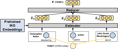
Figure 2: An illustration of our method. It is composed of an estimator and a reducer.

2.2.1 Estimator

For an OOKG entity $e$, given its IKG neighbors $\mathcal{N}_{\mathcal{K}_{\text{aux}}}(e)$ with pretrained embeddings, the estimator aims to compute a set of candidate embeddings. Except TransE and RotatE, other typical KGE models have relatively complex calculations in their translational assumptions. These complex calculations prevent their translational assumptions from deriving specific estimation formulas for OOKG entities. Therefore, we design two sets of estimation formulas based on TransE and RotatE, respectively. To be specific, if $e$ is the head entity, we can obtain its optimal estimation $\widetilde{\mathbf{e}}$ by the following formulas:

$$\widetilde{\mathbf{e}}=\left\{\begin{aligned} &\mathbf{t}-\mathbf{r},&\text{for }\textbf{InvTransE},\\ &\mathbf{t}\circ\mathbf{r}^{-1},&\text{for }\textbf{InvRotatE},\end{aligned}\right.$$

where $\circ$ denotes the element-wise product, $\mathbf{r}^{-1}$ denotes the element-wise inversion.

Otherwise, if $e$ is the tail entity, we can obtain its optimal estimation $\widetilde{\mathbf{e}}$ by the following formulas:

$$\widetilde{\mathbf{e}}=\left\{\begin{aligned} &\mathbf{h}+\mathbf{r},&\text{for }\textbf{InvTransE},\\ &\mathbf{h}\circ\mathbf{r},&\text{for }\textbf{InvRotatE}.\end{aligned}\right.$$

2.2.2 Reducer

After the estimator computes $\left|\mathcal{N}_{\mathcal{K}_{\text{aux}}}(e)\right|$ candidate embeddings, the reducer aims to reduce them to the final embedding of the OOKG entity by weighted average. We design two weighting functions.

Correlation-based weights are query-aware. Inspired by Wang et al. (2019), we first use the conditional probability to model the correlation between two relations:

$$P(r_{2}|r_{1})=\frac{\sum_{e\in\mathcal{E}}{\mathbbm{1}\left(r_{1},r_{2}\in\mathcal{N}_{\mathcal{K}_{\text{train}}}\left(e\right)\right.)}}{\sum_{e\in\mathcal{E}}{\mathbbm{1}\left(r_{1}\in\mathcal{N}_{\mathcal{K}_{\text{train}}}\left(e\right)\right.)}}.$$

When the query relation $r_{q}$ is specified, we assign more weight to the candidate computed via a neighbor with a more relevant relation to $r_{q}$:

$$w_{\text{corr}}(\widetilde{\mathbf{e}})=\frac{P\left(r_{\widetilde{\mathbf{e}}}|r_{q}\right)+P\left(r_{q}|r_{\widetilde{\mathbf{e}}}\right)}{Z_{\text{corr}}},$$

where $Z_{\text{corr}}$ is the normalization factor, $r_{\widetilde{\mathbf{e}}}$ is the neighbor relation via which $\widetilde{\mathbf{e}}$ is computed.

Degree-based weights focus more on the entity with higher degree in the training set:

$$w_{\text{deg}}(\widetilde{\mathbf{e}})=\frac{\log{(d_{\widetilde{\mathbf{e}}}+\delta)}}{Z_{\text{deg}}},$$

where $Z_{\text{deg}}$ is the normalization factor, $d_{\widetilde{\mathbf{e}}}$ is the degree of the neighbor entity via which $\widetilde{\mathbf{e}}$ is computed, $\delta$ is a smoothing factor.

Based on these weighting functions, the final embedding of the OOKG entity $\mathbf{e}$ is computed by

$$\mathbf{e}=\sum_{\widetilde{\mathbf{e}}\in\mathcal{C}}~{}{\widetilde{\mathbf{e}}\cdot w_{\text{corr/deg}}(\widetilde{\mathbf{e}})},$$

where $\mathcal{C}$ denotes the candidate embedding set.

3 Experiments

3.1 Tasks and Datasets

We conduct experiments on two KGC tasks with OOKG entities: link prediction and triplet classification. For link prediction, we use two datasets released by Wang et al. (2019) built based on FB15k (Bordes et al., 2013). For triplet classification, we use nine datasets released by Hamaguchi et al. (2017) built based on WN11 (Socher et al., 2013). All datasets are built for KGC with OOKG entities and composed of a training set, an auxiliary set, a validation set, and a test set. More details of these datasets are included in Appendix.

3.2 Experimental Settings

We tune hyper-parameters for pretraining on the validation set. Generally, we use Adam (Kingma and Ba, 2015) with an initial learning rate of $10^{-3}$ as the optimizer and a batch size of $1,024$. For link prediction, we use an embedding dimension of $1,000$ and the correlation-based weights. For triplet classification, we use an embedding dimension of $300$ and the degree-based weights. Details of experimental settings are included in Appendix.

Method	FB15k-Head-10			FB15k-Tail-10
	MRR	H@10	H@1	MRR	H@10	H@1
GNN-LSTM	0.254	42.9	16.2	0.219	37.3	14.3
GNN-MEAN	0.310	48.0	22.2	0.251	41.0	17.1
LAN	0.394	56.6	30.2	0.314	48.2	22.7
InvTransE	0.462	60.4	38.5	0.357	48.7	29.0
InvRotatE	0.453	60.4	36.9	0.362	49.1	29.3

Table 1: Evaluation results (MRR, Hits@k) of link prediction. Bold is the best. Underline is the second best.

Method	WN11-Head	WN11-Tail	WN11-Both
	3000	3000	1000	3000	5000
ConvLayer	-	-	74.9	-	64.6
FCLEntity	82.6	72.1	-	68.6	-
GNN-LSTM	83.5	71.4	78.5	71.6	65.8
GNN-MEAN	84.3	75.2	83.0	73.3	68.2
LAN	85.2	78.8	83.3	76.9	70.6
InvTransE	87.8	80.1	86.3	78.4	74.6
InvRotatE	86.9	80.1	84.2	75.0	70.6

Table 2: Evaluation results (Accuracy) of triplet classification. Bold is the best. Underline is the second best.

3.3 Baselines

For link prediction, we compare our method with three GNN-based baselines. GNN-MEAN Hamaguchi et al. (2017) uses a mean function to aggregate neighbors. GNN-LSTM adopts LSTM for aggregation. LAN Wang et al. (2019) adopts a both rule- and network-based attention mechanism for aggregation and maintains the best performance so far. For triplet classification, we compare with two more GNN-based baselines. ConvLayer Bi et al. (2020) uses convolutional layers as the transition function. FCLEntity Zhao et al. (2020) uses fully-connected networks as the transition function and adopts an attention-based aggregation.

3.4 Evaluation Metrics

For link prediction, we use Mean Reciprocal Rank (MRR) and the proportion of ground truth entities ranked in top-k (Hits@k, $k\in\left\{1,10\right\}$). All the metrics are filtered versions that exclude false negative candidates. For triplet classification, we use Accuracy. We determine relation-specific thresholds $\delta_{r}$ by maximizing the accuracy on the validation set.

3.5 Main Results

Evaluation results of link prediction are shown in Table 1. From the table, we have the following observations: (1) Both instances of our method significantly outperform all baselines since our estimation formulas are optimal under translational assumptions. (2) GNN-LSTM performs the worst since neighbors are unordered but LSTM captures ordered information. (3) LAN is the best baseline since it adopts a complex attention mechanism to aggregate neighbors more comprehensively. For triplet classification, due to space limitation, we show the main part of the results in Table 2 and the complete results in Appendix. From Table 2, we find that our method outperforms all baselines on all datasets due to our optimal estimation.

Method	MRR	H@10	H@1
InvTransE (Full)	0.462	60.4	38.5
Up to 32 Neighbors	0.447	59.2	37.2
Up to 8 Neighbors	0.386	52.0	31.3
Only 1 Neighbor	0.246	37.9	18.1
Uniform Weights	0.361	52.0	28.1

Table 3: Ablation experiment results for InvTransE on the FB15k-Head-10 dataset of link prediction.

3.6 Analysis

How does the number of neighbors impact the performance? We randomly select up to $k\in\left\{1,8,32\right\}$ IKG neighbors of OOKG entities to use. As shown in Table 3, as the number of used neighbors decreases, the performance drops. This suggests that using more neighbors can enhance the robustness and thus lead to better performance.

Do our weighting functions matter? We attempt to reduce candidates with uniform weights. As shown in Table 3, the performance without our weighting functions drops dramatically. This verifies the effectiveness of our weighting functions.

How does our method perform under increasing OOKG entity ratios? We compare the triplet classification results of InvTransE, LAN, and GNN-MEAN under increasing OOKG entity ratios in Figure 3. We find that, as the OOKG entity ratio increases, the performance of our method drops the slowest. This suggests that our method is more robust to increasing OOKG entity ratios.

Is our method more efficient? We compare InvTransE with LAN to highlight the efficiency of our method. Theoretically, LAN requires $\mathcal{O}(md^{2})$ to represent an entity, where $m$ is the number of neighbors and $d$ is the embedding dimension. By contrast, InvTransE requires only $\mathcal{O}(d)$ and $\mathcal{O}(md)$ to represent an IKG and an OOKG entity, respectively. Empirically, under similar configurations, LAN costs about 15 times the time of InvTransE to train a model for triplet classification. This verifies that our simple method is much more efficient.

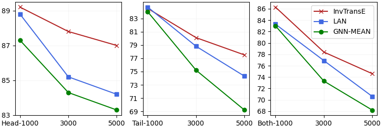
Figure 3: Results under increasing OOKG entity ratios.

4 Related Work

Conventional transductive KGE methods map entities and relations to embeddings, and then use score functions to measure the salience of triplets. TransE (Bordes et al., 2013) pioneers translational distance methods and is the most widely-used one. It derives a series of translational distance methods, such as TransH (Wang et al., 2014), TransR (Lin et al., 2015), and RotatE (Sun et al., 2019). Besides, semantic matching methods form another mainstream (Nickel et al., 2011; Yang et al., 2015; Trouillon et al., 2016; Nickel et al., 2016; Balazevic et al., 2019). These transductive KGE methods achieve success in conventional KGC, but fail to directly represent OOKG entities efficiently.

To represent OOKG entities more efficiently, some inductive methods adopt GNN to aggregate IKG neighbors to inductively produce embeddings for OOKG entities (Hamaguchi et al., 2017; Wang et al., 2019; Bi et al., 2020; Zhao et al., 2020). These methods are effective, but need relatively complex calculations. Other inductive methods incorporate external resources to enrich embeddings and represent OOKG entities via only external resources (Xie et al., 2016; Shi and Weninger, 2018; Xie et al., 2017). However, high-quality external resources are hard and expensive to acquire.

5 Conclusion

This paper aims to address the problem of efficiently representing OOKG entities. We propose a simple and effective method that inductively represents OOKG entities by their optimal estimation under translational assumptions. Given pretrained IKG embeddings, our method needs no additional learning. Experimental results on two KGC tasks with OOKG entities show that our method outperforms the state-of-the-art methods by a large margin with higher efficiency, and maintains a robust performance under increasing OOKG entity ratios.

Appendix A Which Translational Assumptions Can Derive Specific Estimation Formulas for OOKG entities?

For a triplet $(h,r,t)$, translational assumptions of KGE models suppose that $\mathbf{h}$ can establish a connection with $\mathbf{t}$ via an $\mathbf{r}$-specific operation, which can be formulated by the following equation:

$$\mathcal{F}_{\mathbf{r}}(\mathbf{h},\mathbf{t})=0,$$ (1)

where $\mathcal{F}_{\mathbf{r}}(\cdot)$ is an $\mathbf{r}$-specific function that is determined by the specific KGE model. Without loss of generality, we may assume that $h$ is an OOKG entity and $t$ is an IKG entity. Under a translational assumption, we can obtain a specific estimation formula for $\mathbf{h}$ if and only if (1) we regard $\mathbf{h}$ as unknown, and its solution in Equation 1 exists, (2) the solution is unique. If the above two conditions hold, the unique solution of $\mathbf{h}$ is the optimal estimation under the translational assumption, since no other candidate for $\mathbf{h}$ can better fit Equation 1. In the following parts, we analyze translational assumptions of four KGE models (TransE, RotatE, TransH, TransR) as examples.

A.1 TransE

For TransE, its translational assumption is formulated by

$$\mathcal{F}_{\mathbf{r}}(\mathbf{h},\mathbf{t})=\left\|\mathbf{h}+\mathbf{r}-\mathbf{t}\right\|_{1/2}=0.$$ (2)

In this case, we can obtain a unique solution of $\mathbf{h}$ by the following steps:

$$\left\|\mathbf{h}+\mathbf{r}-\mathbf{t}\right\|_{1/2}=0,$$ (3)

$$\Longrightarrow\mathbf{h}+\mathbf{r}-\mathbf{t}=\mathbf{0},$$ (4)

$$\Longrightarrow\mathbf{h}=\mathbf{t}-\mathbf{r}.$$ (5)

This computed $\mathbf{h}$ is the optimal estimation under the translational assumption.

A.2 RotatE

For RotatE, its translational assumption is formulated by

$$\mathcal{F}_{\mathbf{r}}(\mathbf{h},\mathbf{t})=\left\|\mathbf{h}\circ\mathbf{r}-\mathbf{t}\right\|_{1/2}=0.$$ (6)

In this case, we can obtain a unique solution of $\mathbf{h}$ by the following steps:

$$\left\|\mathbf{h}\circ\mathbf{r}-\mathbf{t}\right\|_{1/2}=0,$$ (7)

$$\Longrightarrow\mathbf{h}\circ\mathbf{r}-\mathbf{t}=\mathbf{0},$$ (8)

$$\Longrightarrow\mathbf{h}=\mathbf{t}\circ\mathbf{r}^{-1}.$$ (9)

This computed $\mathbf{h}$ is the optimal estimation under the translational assumption.

A.3 TransH

For TransH, its translational assumption is formulated by

$$\mathcal{F}_{\mathbf{r}}(\mathbf{h},\mathbf{t})=\left\|(\mathbf{h}-\mathbf{w}_{r}^{\top}\mathbf{h}\mathbf{w}_{r})+\mathbf{r}-(\mathbf{t}-\mathbf{w}_{r}^{\top}\mathbf{t}\mathbf{w}_{r})\right\|_{1/2}=0,$$ (10)

where $\mathbf{w}_{r}$ is the unit normal vector of the plane $P$ that $\mathbf{r}$ lies on. From the translational assumption, we can derive the following equations:

$$\left\|(\mathbf{h}-\mathbf{w}_{r}^{\top}\mathbf{h}\mathbf{w}_{r})+\mathbf{r}-(\mathbf{t}-\mathbf{w}_{r}^{\top}\mathbf{t}\mathbf{w}_{r})\right\|_{1/2}=0,$$ (11)

$$\Longrightarrow(\mathbf{h}-\mathbf{w}_{r}^{\top}\mathbf{h}\mathbf{w}_{r})+\mathbf{r}-(\mathbf{t}-\mathbf{w}_{r}^{\top}\mathbf{t}\mathbf{w}_{r})=\mathbf{0},$$ (12)

$$\Longrightarrow(\mathbf{h}-\mathbf{w}_{r}^{\top}\mathbf{h}\mathbf{w}_{r})=(\mathbf{t}-\mathbf{w}_{r}^{\top}\mathbf{t}\mathbf{w}_{r})-\mathbf{r}\triangleq\mathbf{v}.$$ (13)

$\mathbf{h}-\mathbf{w}_{r}^{\top}\mathbf{h}\mathbf{w}_{r}$ is the projection of $\mathbf{h}$ on the plane $P$. From the translational assumption, we can only deduce that the projection of $\mathbf{h}$ is equal to $\mathbf{v}$. However, there exist infinitely many possible $\mathbf{h}$ that can satisfy this condition. Therefore, the solution of $\mathbf{h}$ is not unique, and we cannot obtain a specific estimation formula from the translational assumption of TransH.

A.4 TransR

For TransR, its translational assumption is formulated by

$$\mathcal{F}_{\mathbf{r}}(\mathbf{h},\mathbf{t})=\left\|\mathbf{M}_{r}\mathbf{h}+\mathbf{r}-\mathbf{M}_{r}\mathbf{t}\right\|_{1/2}=0,$$ (14)

where $\mathbf{M}_{r}$ is an r-specific matrix. From the translational assumption, we can derive the following equations:

$$\left\|\mathbf{M}_{r}\mathbf{h}+\mathbf{r}-\mathbf{M}_{r}\mathbf{t}\right\|_{1/2}=0,$$ (15)

$$\Longrightarrow\mathbf{M}_{r}\mathbf{h}+\mathbf{r}-\mathbf{M}_{r}\mathbf{t}=\mathbf{0},$$ (16)

$$\Longrightarrow\mathbf{M}_{r}\mathbf{h}=\mathbf{M}_{r}\mathbf{t}-\mathbf{r}\triangleq\mathbf{v}.$$ (17)

In this case, we derive a system of linear equations from the translational assumption. In this system, there exists a unique solution for $\mathbf{h}$ if and only if the rank of the coefficient matrix $\mathbf{M}_{r}$ is equal to the rank of the augmented matrix $\left[\mathbf{M}_{r};\mathbf{v}\right]$. However, $\mathbf{M}_{r}$ is automatically learned by TransR without this restriction. Therefore, we cannot guarantee that there exists a unique solution for $\mathbf{h}$, and we cannot obtain a specific estimation formula from the translational assumption of TransR.

Appendix B Details of Datasets

Dataset	$\left|\mathcal{K}_{\text{train}}\right|$	$\left|\mathcal{K}_{\text{valid}}\right|$	$\left|\mathcal{K}_{\text{aux}}\right|$	$\left|\mathcal{K}_{\text{test}}\right|$	$\left|\mathcal{R}\right|$	$\left|\mathcal{E}\right|$	$\left|\mathcal{E}^{\prime}\right|$
FB15k-Head-10	108,854	11,339	249,798	2,811	1,170	10,336	2,082
FB15k-Tail-10	99,783	10,190	261,341	2,987	1,126	10,603	1,934
WN11-Head-1000	108,197	4,561	1,938	955	11	37,700	340
WN11-Head-3000	99,963	4,068	5,311	2,686	11	36,646	985
WN11-Head-5000	92,309	3,688	8,048	4,252	11	35,560	1,638
WN11-Tail-1000	96,968	3,864	6,674	852	11	36,771	811
WN11-Tail-3000	78,812	2,851	12,824	2,061	11	33,800	1,874
WN11-Tail-5000	68,040	2,258	15,414	2,968	11	31,311	2,589
WN11-Both-1000	93,683	3,625	7,875	873	11	36,277	1,136
WN11-Both-3000	71,618	2,436	14,453	2,242	11	32,254	2,805
WN11-Both-5000	58,923	1,788	16,660	3,218	11	28,979	3,934

Table 4: Statistics of datasets with OOKG entities. These datasets are built based on FB15k or WN11 and named in the form of “Base-Pos-Num”. Base denotes the based datasets. Pos denotes the position of OOKG entities in test triplets. Num distinguishes different numbers of OOKG entities represented by $\left|\mathcal{E}^{\prime}\right|$.

For link prediction, we use two datasets released by Wang et al. (2019): FB15k-Head-10 and FB15k-Tail-10. These two datasets are built based on FB15k (Bordes et al., 2013). For triplet classification, we use nine datasets released by Hamaguchi et al. (2017): WN11-Head-1000, WN11-Head-3000, WN11-Head-5000, WN11-Tail-1000, WN11-Tail-3000, WN11-Tail-5000, WN11-Both-1000, WN11-Both-3000, and WN11-Both-5000. These nine datasets are built based on WN11 (Socher et al., 2013). Each of the datasets mentioned above is composed of four sets: a training set, an auxiliary set, a validation set, and a test set. Each triplet in the training and validation sets contains only IKG entities. Each triplet in the auxiliary set contains an OOKG entity and an IKG entity. Each triplet in the test set contains at least one OOKG entity. The statistics of the datasets are shown in Table 4.

Appendix C Details of Experimental Settings

Datasets	$d$	$\gamma$	$\alpha$	$n$	L2	Training Steps
FB15k-based	1,000	24.0	1.0	256	N/A	100,000
WN11-based	300	0.5	1.0	128	$10^{-5}$	20,000

Table 5: Hyper-parameters for two categories of datasets. We use the same hyper-parameters for two FB15k-based datasets and the same hyper-parameters for nine WN11-based datasets. On each dataset, we use the same hyper-parameters for two pretrained models. $d$ denotes the embedding dimension. $\gamma$ denotes the margin. $\alpha$ denotes the sampling temperature. $n$ denotes the negative sampling size. L2 denotes the parameter of L2 regularization, where N/A means no regularization.

To pretrain the TransE and RotatE models, we adopt the self-adversarial negative sampling loss proposed by Sun et al. (2019) in consideration of its good performance on training TransE and RotatE. The self-adversarial negative sampling loss $L$ is formulated as

$$L=-\log\sigma\left(\gamma-\mathcal{D}\left(\mathbf{h},\mathbf{r},\mathbf{t}\right)\right)-\sum_{i=1}^{n}~{}p\left(h_{i}^{\prime},r,t_{i}^{\prime}\right)\log\sigma\left(\mathcal{D}\left(\mathbf{h}_{i}^{\prime},\mathbf{r},\mathbf{t}_{i}^{\prime}\right)-\gamma\right),$$

where $\sigma$ is the sigmoid function, $\gamma$ is the margin, $n$ is the negative sampling size and $\left(h_{i}^{\prime},r,t_{i}^{\prime}\right)$ is the i-th negative sample triplet. $\mathcal{D}\left(\cdot\right)$ is the distance function. $\mathcal{D}\left(\mathbf{h},\mathbf{r},\mathbf{t}\right)$ is equal to $\left\|\mathbf{h}+\mathbf{r}-\mathbf{t}\right\|_{1/2}$ for TransE and is equal to $\left\|\mathbf{h}\circ\mathbf{r}-\mathbf{t}\right\|_{1/2}$ for RotatE. $p$ is the self-adversarial weight function which gives more weight to the high-scored negative samples:

$$p\left(h_{i}^{\prime},r,t_{i}^{\prime}\right)\propto\exp\left(\alpha\cdot\mathcal{F}\left(\mathbf{h}_{i}^{\prime},\mathbf{r},\mathbf{t}_{i}^{\prime}\right)\right),$$

where $\alpha$ is a hyper-parameter called sampling temperature to be tuned. $\mathcal{F}(\cdot)$ is the score function that is equal to $-\mathcal{D}(\cdot)$.

We conduct each experiment on a single Nvidia Geforce GTX-1080Ti GPU and tune hyper-parameters on the validation set. Generally, we set the batch size to $1024$ and use Adam (Kingma and Ba, 2015) with an initial learning rate of $10^{-3}$ as the optimizer. We choose the correlation-based weights for link prediction and choose the degree-based weights with a smoothing factor of $0.1$ for triplet classification. Other hyper-parameters are shown in Table 5.

Appendix D Complete Evaluation Results of Triplet Classification

Method	WN11-Head			WN11-Tail			WN11-Both
	1000	3000	5000	1000	3000	5000	1000	3000	5000
ConvLayer	-	-	-	-	-	-	74.9	-	64.6
FCLEntity	-	82.6	-	-	72.1	-	-	68.6	-
GNN-LSTM	87.0	83.5	81.8	82.9	71.4	63.1	78.5	71.6	65.8
GNN-MEAN	87.3	84.3	83.3	84.0	75.2	69.2	83.0	73.3	68.2
LAN	88.8	85.2	84.2	84.7	78.8	74.3	83.3	76.9	70.6
InvTransE	89.2	87.8	87.0	84.5	80.1	77.5	86.3	78.4	74.6
InvRotatE	88.6	86.9	86.5	84.7	80.1	75.8	84.2	75.0	70.6

Table 6: Complete evaluation results (Accuracy) of triplet classification. Bold is the best. Underline is the second best. The results of all five baselines are taken from their original papers.

References

- Balazevic et al. (2019) Ivana Balazevic, Carl Allen, and Timothy M. Hospedales. 2019. TuckER: Tensor factorization for knowledge graph completion. In EMNLP-IJCNLP 2019, pages 5184–5193.
- Bi et al. (2020) Zhongqin Bi, Tianchen Zhang, Ping Zhou, and Yongbin Li. 2020. Knowledge transfer for out-of-knowledge-base entities: Improving graph-neural-network-based embedding using convolutional layers. IEEE Access, 8:159039–159049.
- Bordes et al. (2013) Antoine Bordes, Nicolas Usunier, Alberto Garcia-Duran, Jason Weston, and Oksana Yakhnenko. 2013. Translating embeddings for modeling multi-relational data. In NeurIPS 2013, pages 2787–2795.
- Hamaguchi et al. (2017) Takuo Hamaguchi, Hidekazu Oiwa, Masashi Shimbo, and Yuji Matsumoto. 2017. Knowledge transfer for out-of-knowledge-base entities: A graph neural network approach. In IJCAI 2017, pages 1802–1808.
- Kingma and Ba (2015) Diederik P Kingma and Jimmy Ba. 2015. Adam: A method for stochastic optimization. In ICLR 2015.
- Lin et al. (2015) Yankai Lin, Zhiyuan Liu, Maosong Sun, Yang Liu, and Xuan Zhu. 2015. Learning entity and relation embeddings for knowledge graph completion. In AAAI 2015, pages 2181–2187.
- Nickel et al. (2016) Maximilian Nickel, Lorenzo Rosasco, and Tomaso A. Poggio. 2016. Holographic embeddings of knowledge graphs. In AAAI 2016, pages 1955–1961.
- Nickel et al. (2011) Maximilian Nickel, Volker Tresp, and Hans-Peter Kriegel. 2011. A three-way model for collective learning on multi-relational data. In ICML 2011, pages 809–816.
- Shi and Weninger (2018) Baoxu Shi and Tim Weninger. 2018. Open-world knowledge graph completion. In AAAI 2018, pages 1957–1964.
- Socher et al. (2013) Richard Socher, Danqi Chen, Christopher D Manning, and Andrew Ng. 2013. Reasoning with neural tensor networks for knowledge base completion. In NeurIPS 2013, pages 926–934.
- Sun et al. (2019) Zhiqing Sun, Zhi-Hong Deng, Jian-Yun Nie, and Jian Tang. 2019. RotatE: Knowledge graph embedding by relational rotation in complex space. In ICLR 2019.
- Trouillon et al. (2016) Théo Trouillon, Johannes Welbl, Sebastian Riedel, Éric Gaussier, and Guillaume Bouchard. 2016. ComplEx embeddings for simple link prediction. In ICML 2016, pages 2071–2080.
- Wang et al. (2019) Peifeng Wang, Jialong Han, Chenliang Li, and Rong Pan. 2019. Logic attention based neighborhood aggregation for inductive knowledge graph embedding. In AAAI 2019, pages 7152–7159.
- Wang et al. (2014) Zhen Wang, Jianwen Zhang, Jianlin Feng, and Zheng Chen. 2014. Knowledge graph embedding by translating on hyperplanes. In AAAI 2014, pages 1112–1119.
- Xie et al. (2016) Ruobing Xie, Zhiyuan Liu, Jia Jia, Huanbo Luan, and Maosong Sun. 2016. Representation learning of knowledge graphs with entity descriptions. In AAAI 2016, pages 2659–2665.
- Xie et al. (2017) Ruobing Xie, Zhiyuan Liu, Huanbo Luan, and Maosong Sun. 2017. Image-embodied knowledge representation learning. In IJCAI 2017, pages 3140–3146.
- Yang et al. (2015) Bishan Yang, Wen-tau Yih, Xiaodong He, Jianfeng Gao, and Li Deng. 2015. Embedding entities and relations for learning and inference in knowledge bases. In ICLR 2015.
- Zhao et al. (2020) Ming Zhao, Weijia Jia, and Yusheng Huang. 2020. Attention-based aggregation graph networks for knowledge graph information transfer. In PAKDD 2020, pages 542–554.