Unified description of the coupled-channels and statistical Hauser-Feshbach nuclear reaction theories for low energy neutron incident reactions

Abstract

We incorporate the coupled-channels optical model into the statistical Hauser-Feshbach nuclear reaction theory, where the scattering matrix is diagonalized by performing the Engelbrecht-Weidenmüller transformation. This technique has been implemented in the coupled-channels optical model code ECIS by J. Raynal, and we extend this method so that all the open channels in a nucleon-induced reaction on a deformed nucleus can be calculated consistently.

1 Introduction

It is well known that the nucleon-induced scattering process from a nucleus can be described by the optical model, where the imaginary part of the potential represents a deficit of incoming flux, hence the scattering $S$-matrix of the optical model is no longer unitary. At relatively low incident energies, where only a few open channels are involved, an absorbed particle once forms a compound state in the target nucleus, and it comes back to the entrance channel as the compound elastic scattering process. The total wave-function is the coherent sum of the incoming and out-going waves Moldauer1961 ; Moldauer1964 . Although the direct (or “shape”) elastic scattering $(d\sigma/d\Omega)^{\rm SE}$ and the compound elastic scattering $(d\sigma/d\Omega)^{\rm CE}$ cannot be distinguished experimentally, theoretical interpretation divides these two scattering processes into different time-scale domains — the fast and slow parts. The optical model gives the faster part, while the statistical model for nuclear reactions Kawai1973 ; Hofmann1975 ; Moldauer1980 ; Verbaarschot1985 ; Kawano2015 accounts for the slower compound elastic scattering process. We understand the experimental elastic scattering data are the incoherent sum of both processes. The optical model codes, which have been utilized to analyze the nucleon scattering data, for example ECIS Raynal1972 , ELIESE-3 JAERI-1224 , CASTHY JAERI-1321 , ABAREX ANLNDM145 , and so forth, are capable for calculating the compound nucleus (CN) process, yet they are limited to a binary reaction with relatively small channel space. Note that the aforementioned codes are just examples, and there exist more computer programs that calculate the optical model in the nuclear science field.

As a general descriptions of nuclear reaction process, the Hauser-Feshbach (HF) statistical theory Hauser1952 is extended to a multi-stage reaction, where a residual nucleus formed after particle emission is allowed to further decay as another CN process. In this case, the main part of the calculation is the compound nuclear reaction, and the optical model is somewhat hidden behind it. The so-called HF codes, GNASH LA6947 ; LA12343 , TNG ORNL-7042 , STAPRE IRK-76 , EMPIRE INDC0603 , TALYS Koning2004 ; Koning2012 and so on, invoke an optical model code to generate transmission coefficients $T_{lj}$ as a model input, where the quantum numbers $lj$ are the orbital angular momentum and the spin. J. Raynal’s ECIS code has been widely used for this purpose. Exceptions are the CCONE Iwamoto2007 ; Iwamoto2013 and CoH₃ Kawano2010 ; Kawano2019 codes, those include a private $T_{lj}$ generator internally.

These HF codes, despite they are capable for calculating nuclear reaction cross sections for all the open channels, do not furnish a strict connection between the optical and statistical models. This issue becomes more serious when the target nucleus is strongly deformed, and the single channel optical model has to be extended to the coupled-channels (CC) formalism Tamura1965 . There are two vague approximations made by these codes to deal with the nuclear deformation effect; (a) $T_{lj}$ for the excited states are replaced by the one for the ground state by correcting the channel energy, and (b) the direct reaction effect in the statistical theory Hofmann1975 ; Engelbrecht1973 ; Moldauer1975b is ignored. Raynal carefully dealt with these issues in ECIS, and established a unique integration of the optical and HF statistical models, nevertheless the formalism was limited to the binary reactions only.

Like ECIS or ELIESE-3, CoH was originally developed as a nucleon scattering data analysis code Kawano1999c , which includes the statistical HF theory with the width fluctuation correction by Moldauer Moldauer1980 . Later, CoH was extended to the full multi-stage HF code, so that the optical model and the statistical model were naturally unified just like ECIS, but in more general sense. In this paper we present the unified description of CC optical and HF statistical models implemented in the CoH₃ code, where Raynal’s ideas in ECIS were important resources and clues. We demonstrate how the approximations made by the existing HF codes bring systematic uncertainties in the predicted cross sections. We limit ourselves to the low energy neutron induced reactions only, where the compound elastic scattering plays more important role than the charged-particle cases.

2 Theoy

2.1 Compound nuclear reaction and transmission coefficient

The energy-averaged cross section for a reaction from channel $a$ to channel $b$ is written by the partial decay width $\Gamma_{c}$ as

$$\sigma^{\rm CN}_{ab}=\frac{\pi}{k_{a}^{2}}g_{a}\frac{2\pi}{D}\left\langle\frac{\Gamma_{a}\Gamma_{b}}{\sum_{c}\Gamma_{c}}\right\rangle\ ,$$ (1)

where $D$ is the average resonance spacing, $k_{a}$ is the wave number of incoming particle, and $g_{a}$ is the spin factor given later. By applying a relation between the single-channel transmission coefficient $T_{a}$ and the decay width $\Gamma_{a}$,

$$T_{a}\simeq 2\pi\frac{\langle\Gamma_{a}\rangle}{D}\ ,$$ (2)

the width fluctuation corrected HF cross section Moldauer1961 ; Hauser1952 reads

$$\sigma^{\rm CN}_{ab} = \frac{\pi}{k_{a}^{2}}g_{a}\frac{T_{a}T_{b}}{\sum_{c}T_{c}}W_{ab}$$ (3)

$$= \sigma^{\rm HF}_{ab}W_{ab}\ ,$$

where $\sigma^{\rm HF}_{ab}$ is the original HF cross section. The width fluctuation correction factor $W_{ab}$ is also a function of $T_{a}$. When the resonance decay width $\Gamma_{a}$ forms the $\chi^{2}$ distribution with the channel degree-of-freedom $\nu_{a}$, the width fluctuation correction factor can be evaluated numerically as Moldauer1975b ; Moldauer1975a ; Moldauer1976

$$W_{ab} = \left(1+\frac{2\delta_{ab}}{\nu_{a}}\right)\int_{0}^{\infty}\!\!\!\frac{dt}{F_{a}(t)F_{b}(t)\prod_{k}F_{k}(t)^{\nu_{k}/2}},$$ (4)

$$F_{k}(t) = 1+\frac{2}{\nu_{k}}\frac{T_{k}}{\sum_{c}T_{c}}t\ .$$ (5)

The Gaussian Orthogonal Ensemble (GOE) model Verbaarschot1985 provides accurate estimates of $\nu_{a}$ Moldauer1980 ; Kawano2015 in terms of $T_{a}$, and all of the reaction cross sections $\sigma_{ab}$ are determined by $T_{a}$ and $T_{b}$ only.

When the ground state of nucleus does not couple so strongly with other states by collective excitation, the scattering matrix element $S_{aa}$ is given by solving the single-channel Schrödinger equation for a spherical optical potential. Because the $S$-matrix is diagonal, the transmission coefficient $T_{a}$ is defined as a unitarity deficit

$$T_{lj}=1-|S_{lj,lj}|^{2}\ ,$$ (6)

where we denote the channel quantum numbers explicitly by the orbital angular momentum $l$, and spin $j$. We also add a discrete level index $n$ as $T_{lj}^{(n)}$. $T_{lj}^{(0)}$ stands for a probability to form a CN state from the ground state. The detailed-balance equation in Eq. (3) is schematically shown in Fig. 1 for the two level case. $T_{lj}^{(1)}$ stands for a probability to form the same CN from the first excited state. However, since optical potentials for excited nuclei are usually unknown, they are replaced by $T_{lj}^{(0)}$ and shift the energy by the excitation energy $E_{x}^{(n)}$ to take account of the energy difference,

$$T_{lj}^{(n)}(E)\simeq T_{lj}^{(0)}(E-E_{x}^{(n)})\ .$$ (7)

There exist many phenomenological global optical potentials that are energy-dependent, and the assumption of Eq. (7) enables all of the HF codes to perform cross section calculations in wide energy and target-mass ranges. In fact, almost all of the HF codes generate $T_{lj}^{(0)}$ on a fixed energy grid before performing a CN calculation, and interpolate $T_{lj}^{(0)}$ to obtain a required value at each energy point.

Figure 1: The ground and excited states in a target nucleus and the compound nucleus (CN) connected by the particle transmission coefficients, $T_{lj}^{(0)}$ and $T_{lj}^{(1)}$. $T_{lj}^{(1)}$ is often approximated by shifting to the ground state, as shown by the dotted arrow.

2.2 Coupled-channels transmission coefficient

When strongly coupled collective levels are involved in the target system, Eq. (3) must be calculated by the transmission coefficients in the CC formalism, and the $S$-matrix is no longer diagonal. ECIS and CoH₃ calculate generalized transmission coefficients for all the included states from the CC $S$-matrix Kawano2009 . The time-reversal symmetry of $S$-matrix yields the transmission coefficient for all of the $n$-th excited state simultaneously as

$$T_{lj}^{(n)} = \sum_{J\Pi}\sum_{a}{{2s+1}\over{2j_{a}+1}}g_{J}\left(1-\sum_{b}|S_{ab}^{J\Pi}|^{2}\right)$$ (8)

$$\times \delta_{n_{a},n}\delta_{l_{a},l}\delta_{j_{a},j}\ ,$$

where $J\Pi$ is the total spin and parity. This is shown in Fig. 2. The spin-factor $g_{J}$ is given by

$$g_{J}={{2J+1}\over{(2s+1)(2I_{n}+1)}},$$ (9)

where $s$ is the intrinsic spin of the projectile (= 1/2 for neutron), and $I_{n}$ is the target spin of $n$-th level. The summation runs over the parity conserved channels, albeit we omit a trivial parity conservation. In this expression, cross sections to the directly coupled channels are eliminated to ensure the sum of $T_{ij}^{(n)}$ gives a correct CN formation cross section from the $n$-th level

$$\sigma_{R}^{(n)} = {{\pi}\over{k_{n}^{2}}}\sum_{J\Pi}\sum_{a}\delta_{n_{a},n}g_{J}\left(1-\sum_{b}|S_{ab}^{J\Pi}|^{2}\right)$$ (10)

$$= {{\pi}\over{k_{n}^{2}}}\sum_{lj}{{2j+1}\over{2s+1}}T_{lj}^{(n)}.$$

Now the off-diagonal elements in the $S$-matrix are effectively eliminated. By substituting $T_{lj}^{(n)}$ into Eq. (3), the HF cross section is determined in terms of the detailed balance. This formulation is, however, valid only when the width fluctuation correction is not so significant, because the off-diagonal elements in $S$ to calculate $W_{ab}$ are ignored. We will discuss this later.

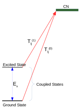
Figure 2: In the coupled-channels method, the transmission coefficients $T_{lj}^{(0)}$ and $T_{lj}^{(1)}$ can be derived simultaneously from the $S$-matrix.

The HF codes, exept for ECIS and CoH₃ to our knowledge, simplify Eq. (8) by applying the approximation of Eq. (7), namely $T_{lj}^{(n)}(E)\simeq T_{lj}^{(0)}(E-E_{x}^{(n)})$, hence all the CC $S$-matrix properties are lost. To examine this approximation, we calculate transmission coefficients for the excited states $T_{lj}^{(n)}(E)$ and compare with those for the energy-shifted ground state $T_{lj}^{(0)}(E-E_{x}^{(n)})$. The comparison includes two cases of rotational band head; the target ground state spin is zero, and it is half-integer. The first example is for the fast-neutron induced reaction on ²³⁸U, in which we couple 5 levels (0, 45, 148, 307, and 518 keV, from $0^{+}$ to $8^{+}$) in the ground state rotational band. The optical potential of Soukhovitskii et al. Soukhovitskii2004 is used. A natural choice for the second case, the half-integer ground state spin, is ²³⁹Pu. However, its large fission cross sections at low energies blur the difference coming from the definition of $T_{lj}$. Instead, we adopt ¹⁶⁹Tm that has a similar level structure to ²³⁹Pu Kawano2009 . The coupled levels are 0, 8.4, 118, 139, and 332 keV from $(1/2)^{+}$ to $(9/2)^{+}$, and the optical potential of Kunieda et al. Kunieda2007 is employed.

Figure 3 shows the difference in the $l=0$ and 1 transmission coefficients for ²³⁸U. The approximation by $T_{lj}^{(0)}$ seems to be reasonable for the $s$-wave transmission coefficient, while the difference reaches about 10% for the $p$-wave case. The calculations for ¹⁶⁹Tm, shown in Fig. 4, show the opposite tendency; a notable difference appears in the $s$-wave. It is difficult to draw a general conclusion by these limited examples. However, it is obvious that the calculated cross sections by feeding these transmission coefficients into the statistical HF theory are no longer equivalent, and the energy-shifted transmission coefficient inflates uncertainty in the calculated results.

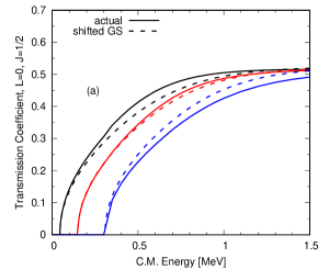
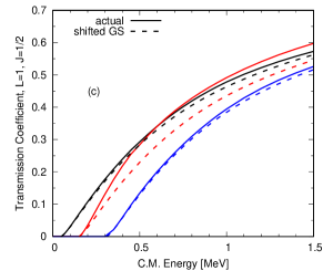
Figure 3: Calculated transmission coefficients for the first and second coupled levels of ²³⁸U; (a) for $(l,j)=(0,1/2)$, (b) $(1,3/2)$, and (c) $(1,1/2)$. The solid curves are the actual transmission coefficient given by the CC $S$-matrix. The dashed curves are approximation by the ground state transmission coefficient shifted by the level excitation energies. The black, red, and blue curves are for the first, second, and third levels. The corresponding level should also be distinguished by the shifted threshold energies.

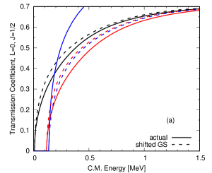
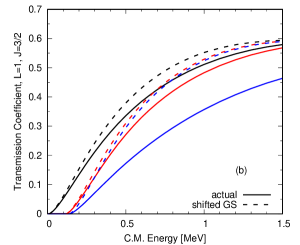
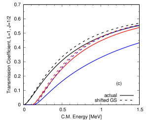
Figure 4: Same as Fig. 3 but for ¹⁶⁹Tm.

2.3 Generalized transmission coefficient in compound inelastic scattering calculation

To see the actual impact of the generalized transmission coefficients on the cross section calculation, we have to calculate the HF equation with these actual/approximated transmission coefficients. Unfortunately, this is not so easy in general, because it requires extensive modification to the computer programs. Instead, we made an ad-hoc modification to CoH₃ to test this. For a 100-keV neutron induced reaction on ²³⁸U, CoH₃ with the generalized transmission coefficient gives the inelastic scattering cross section of 553 mb to the 45 keV $2^{+}$ level. At this energy, an equivalent center-of-mass (CMS) energy to the first 45 keV level is $100A/(A+1)-44.9=54.7$ keV. We calculate $T_{lj}^{(0)}$ at $E_{\rm CMS}=54.7$ keV, and replace $T_{lj}^{(1)}$ by these values. The calculated inelastic scattering cross section is 488 mb, which is 9% smaller than the generalized transmission case, and closer to the evaluated value in JENDL-4 Iwamoto2007 ; JENDL4 of 461 mb. This observation is consistent with the larger $p$-wave transmission coefficient as shown in Fig. 3 (b).

In the past, a code comparison was carried out Capote2017 by including EMPIRE INDC0603 , TALYS Koning2012 ; Koning2008 , CCONE Iwamoto2016 , and CoH₃. The result revealed that the inelastic scattering cross section by CoH₃ tends to be higher than those by the other codes for the ²³⁸U case at low energies. The difference is about 10% at 100 keV, and this confirms our numerical exercise here; the approximation by the ground state transmission coefficient systematically underestimates the inelastic scattering cross section for the ²³⁸U case.

2.4 Transmission coefficient for uncoupled channels

There might be many uncoupled levels involved in actual CN calculations, as schematically shown in Fig. 5. In the target nucleus, there are uncoupled discrete levels up to some critical energy, then a level density model is used to discretize the continuum above there. The transmission coefficients to these states are calculated by the single-channel case.

The formed CN state can decay by emitting a charged-particle, $\gamma$-ray or fission. The charged-particle transmission coefficients are basically the same as the uncoupled neutron channel case, except for the Coulomb interaction. The transmission coefficients for the $\gamma$ decay are calculated by applying the giant dipole resonance (GDR) model Goriely2019 , where GDR parameters derived from experimental data or theoretically predicted are often tabulated Goriely2019 ; Kawano2020 . Although there are a large number of final states available after a $\gamma$-ray emission, these probabilities are very small compare to the neutron transmission coefficients. Often it is good enough to lump the $\gamma$-ray channels into a single $\gamma$-ray transmission coefficient as

$$T_{\gamma}=\sum_{XL}\int_{0}^{E_{n}+S_{n}}T_{XL}(E_{\gamma})\rho(E_{x})dE_{x}\ ,$$ (11)

where $S_{n}$ is the neutron separation energy, $X$ stands for the type of radiation (E: electric, M: magnetic), $L$ is the multipolarity, and $\rho(E_{x})$ is the level density at excitation energy $E_{x}=E_{n}+S_{n}-E_{\gamma}$. When the final state is in a discrete level, the integration in Eq. (11) is replaced by an appropriate summation.

When the CN fissions, the simplest expression of the fission transmission coefficients is the WKB approximation to the inverted parabola shape of fission barriers proposed by Hill and Wheeler Hill1953 . Albeit it is know that this form has an issue to reproduce experimental fission cross sections, this is beyond the scope of current paper, and we do not discuss it further. The fission takes place though many states on top of the fission barrier, so that it is convenient to lump these partial fission probabilities into the fission transmission coefficient $T_{f}$.

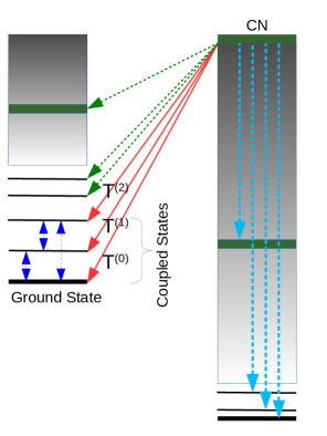
Figure 5: All the possible decay channels from a compound state are schematically shown by the arrows. The solid arrows are the transmission coefficients by the CC model. All the other channels shown by the dotted arrows are uncoupled levels.

2.5 Engelbrecht-Weidenmüller transformation for width fluctuation correction

The width fluctuation correction factor $W_{ab}$ consists of the elastic enhancement factor and the actual width fluctuation correction factor Moldauer1975a . A convenient definition is suggested by Hilaire, Lagrange, and Koning Hilaire2003 , which is to define as a ratio to the pure HF cross section as in Eq. (3). When we ignore the channel coupling effect, $W_{ab}$ in Eq. (4) can be calculated by the generalized transmission coefficients in Eq. (8). However, we cannot employ this prescription when a strong channel-coupling results in non-negligible off-diagonal elements in $S$. Instead, we perform the Engelbrecht-Weidenmüller (EW) transformation Engelbrecht1973 to correctly eliminate the off-diagonal elements.

Satchler’s transmission matrix Satchler1963 is defined by the CC $S$-matrix as

$$P_{ab}=\delta_{ab}-\sum_{c}S_{ac}S_{bc}^{*}\ .$$ (12)

Since $P$ is Hermitian, we can diagonalize this by a unitary transformation Engelbrecht1973

$$(UPU^{\dagger})_{\alpha\beta}=\delta_{\alpha\beta}p_{\alpha},\qquad 0\leq p_{\alpha}\leq 1\ ,$$ (13)

where $\alpha$ and $\beta$ are the channel indices in the diagonalized space. The diagonal element $p_{\alpha}$ is the new transmission coefficient, because the $S$-matrix is also diagonalized as

$$\tilde{S}=USU^{T}\ ,$$ (14)

which defines the single-channel transmission coefficient

$$T_{\alpha}=1-\left|\tilde{S}_{\alpha\alpha}\right|^{2}=p_{\alpha}\ .$$ (15)

We now calculate the width fluctuation in the diagonal channel space, then transform back to the cross-section space by Hofmann1975

$$\sigma_{ab} = \sum_{\alpha}|U_{\alpha a}|^{2}|U_{\alpha b}|^{2}\sigma_{\alpha\alpha}$$ (16)

$$+ \sum_{\alpha\neq\beta}U_{\alpha a}^{*}U_{\beta b}^{*}\left(U_{\alpha a}U_{\beta b}+U_{\beta a}U_{\alpha b}\right)\sigma_{\alpha\beta}$$

$$+ \sum_{\alpha\neq\beta}U_{\alpha a}^{*}U_{\alpha b}^{*}U_{\beta a}U_{\beta b}\left\langle{\tilde{S}_{\alpha\alpha}\tilde{S}_{\beta\beta}^{*}}\right\rangle.$$

$\sigma_{\alpha\alpha}$ and $\sigma_{\alpha\beta}$ are the width fluctuation corrected cross section with the transmission coefficient of $p_{\alpha}$. The last term $\left\langle{\tilde{S}_{\alpha\alpha}\tilde{S}_{\beta\beta}^{*}}\right\rangle$ was evaluated by applying the Monte Carlo technique to GOE Kawano2016 ,

$$\overline{\tilde{S}_{\alpha\alpha}\tilde{S}_{\beta\beta}^{*}}\simeq e^{i(\phi_{\alpha}-\phi_{\beta})}\left(\frac{2}{\nu_{\alpha}}-1\right)^{1/2}\left(\frac{2}{\nu_{\beta}}-1\right)^{1/2}\sigma_{\alpha\beta},\\$$ (17)

where $\phi_{\alpha}=\tan^{-1}\tilde{S}_{\alpha\alpha}$. Here we replaced the energy average $\left\langle{*}\right\rangle$ by the ensemble average $\overline{*}$. Applying the GOE model to the channel degree-of-freedom $\nu_{\alpha}$ Kawano2015 , the HF cross section with the width fluctuation correction is fully characterized in the CC framework.

When uncoupeld-channels, such as the inelastic scattering to the higher levels, $\gamma$-decay and fission channels, exist, the transmission matrix has these sub-space

$$P=\left(\begin{array}[]{cccc}P_{\rm C}&&&\\ &T_{n}&&\\ &&T_{\gamma}&\\ &&&T_{f}\\ \end{array}\right),$$ (18)

where $P_{\rm C}$ is the coupled channels $P$ matrix in Eq. (12). Because $T_{n}$, $T_{\gamma}$, and $T_{f}$ are still diagonal, the unitary transformation is only applied to $P_{\rm C}$. The uncoupled cross section is calculated by Kawano2016

$$\sigma_{ab}=\sum_{\alpha}|U_{\alpha a}|^{2}\sigma_{\alpha\beta}\delta_{\beta b}\ .$$ (19)

Here we take ²³⁸U and ¹⁶⁹Tm as examples again. The width fluctuation correction is defined as a ratio to the HF cross section, and we calculate two cases; (a) the width fluctuation factor $W_{ab}$ in Eq. (4) is calculated by using the generalized transmission coefficient of Eq. (8), and the off-diagonal elements in the $S$-matrix are ignored, and (b) the full EW transformation is performed.

It is known that an asymptotic value of $W_{aa}$ (elastic enhancement factor) is 2 when all the channels are equivalent. Figure 6 (a), which is the calculated $W_{aa}$ for ²³⁸U, shows this behavior, but the EW transformation slightly deters $W_{aa}$ from approaching the asymptote. The weaker elastic enhancement results in increase in the inelastic scattering channels. This is also demonstrated by the Monte Carlo simulation for the GOE scattering matrix when direct reaction components are involved Kawano2015 . In other words, the directly coupled channels squeeze the elastic scattering channel due to constraint by the $S$-matrix unitarity, hence the enhancement in the elastic channel will have less influence on the other channels.

In the case of ¹⁶⁹Tm, shown in Fig. 7, the asymptotic value of $W_{aa}$ does not reach 2 but stays about 1.6. This might be because the $s$-wave transmission coefficient for the second excited state is very different from the other channels. Because the number of channels is larger than the ²³⁸U case, the EW transformation less impacts the CN calculations. In addition, other uncoupled channels, e.g. radiative capture and fission channels if exist, further mitigate the elastic enhancement effect. Therefore the EW transformation is mostly important for rotating even-even nuclei with large deformation. Having said that, the difference seen in Fig. 7 implies an inherent deficiency in the simplified HF calculations widely adopted nowadays.

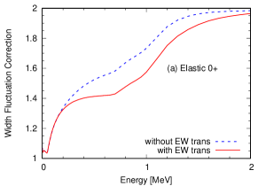
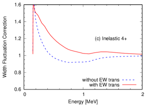
Figure 6: Width fluctuation corrections for ²³⁸U defined as a ratio to the Hauser-Feshbach cross section. The panels (a), (b), and (c) are the compound elastic, inelastic to the first, and second levels for the neutron-induced reaction on ²³⁸U. The solid curves are calculated by performing the Engelbrecht-Weidenmüller (EW) transformation, and the dashed curves are without the EW transformation.

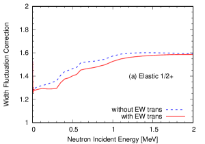
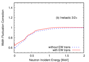
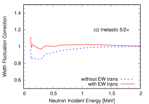
Figure 7: Same as Fig. 6 but for ¹⁶⁹Tm.

3 Application

In reality, the EW transformation does not modifies the calculated cross sections so largely. As seen in Fig. 6, the difference between the EW and single-channel $W_{ab}$ cases is at most 15%. Such a difference may occur due to other uncertain inputs to the calculation. One of the most crucial model parameters is the optical potential. The optical potential parameters are often obtained phenomenologically by fitting to experimental elastic scattering and total cross sections. In general, similar quality of data fitting can be achieved by different potential parameters, while they may have slightly different partial wave contributions. Fluctuation in the partial wave contribution is sometimes visible in the inelastic scattering cross sections, where limited numbers of partial waves are involved.

Figure 8 (a) shows a comparison of the calculated inelastic scattering cross section to the first 45 keV level of ²³⁸U with available experimental data of Miura et al. Miura2000 , Kornilov and Kagalenko Kornilov1995 , Moxon et al. Moxon1994 , Litvinskii et al. Litvinskii1990 , Winters et al. Winters1981 , Guenther et al. ANLNDM16 , Haouat et al. Haouat1982 , and Tsang and Brugger Tsang1978 . We performed this calculation with the CC optical model potential of Soukhovitskii et al. Soukhovitskii2004 . While the measurements are largely scattered in the hundreds keV region, the EW transformation moves the calculation into a preferable direction. However, the enhancement due to the EW transformation is rather modest, which is also seen in Fig. 6 (b).

When we switch the optical potential into the updated Soukhovitskii potential Soukhovitskii2005 , the EW transformation becomes noticeable as shown in Fig. 8 (b). In this case the enhancement is visible in the wider energy range. Of course it is not rational to verify an optical potential by applying it to the statistical model, as ambiguity caused by other model inputs persists. In the CC formalism, calculated cross sections are also influenced by the coupling scheme Dietrich2012 . Despite other available optical potentials for ²³⁸U may provide different excitation functions of 45-keV level, we may say generally that the EW transformation increases the 45-keV level cross section due to the hindered elastic enhancement.

The increase in the inelastic scattering of the 148-keV level, as well as the total inelastic scattering cross section, is shown in Fig. 9. The $2^{+}$ cross sections are the same as those in Fig. 8. Since the relative magnitude of the $4^{+}$ level cross section is smaller than the $2^{+}$ level, this has a minor impact on the total inelastic scattering cross section. This is also true for the higher spin states ($6^{+},8^{+}\ldots$)

It might be worth reminding that these “without EW” cases employ the generalized transmission coefficient to calculate both the HF cross section and the $W_{ab}$ factor. When one adopts a conventional prescription of $T^{(n)}(E)\simeq T^{(0)}(E-E_{x}^{(n)})$, the calculated inelastic scattering cross section would be further lower than the no-EW case. Evidently this approximation cannot be justified anymore when the nuclear deformation plays an important role. Use of the generalized transmission calculation is still approximated, albeit it mitigates this deficiency to some extent, and afford us not so heavy computation. However, as we demonstrated the quantitative deficiencies in the approximations and simplifications made so far, we should consider implementing the EW transformation in the HF model codes for better prediction of nuclear reaction cross sections for deformed nuclei.

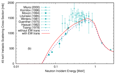
Figure 8: Comparison of calculated inelastic scattering cross section to the first 45 keV level of ²³⁸U. The top panel (a) is the case of 2004 Soukhovitskii potential Soukhovitskii2004 , and (b) is the 2005 Soukhovitskii potential Soukhovitskii2005

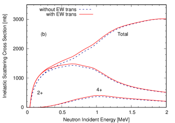
Figure 9: The inelastic scattering cross section to the 45 keV and 148 keV levels, and the total inelastic scattering cross section of ²³⁸U. The top panel (a) is for the 2004 Soukhovitskii potential Soukhovitskii2004 , and (b) is the 2005 Soukhovitskii potential Soukhovitskii2005

A remaining complication is the angular distributions of scattered particles in the CN process. The differential cross section is expanded by the Legendre polynomials in the Blatt-Biedenharn formalism Blatt1952 ,

$$\left(\frac{d\sigma}{d\Omega}\right)_{ab}=\sum_{L}B_{L}P_{L}(\cos\theta_{b})\ ,$$ (20)

where the scattering angle $\theta_{b}$ is in the center-of-mass system. A full expression of the $B_{L}$ coefficients is given in the single-channel width fluctuation case Moldauer1964 ; Kim2020 . However, a complete formulation of the $B_{L}$ coefficient becomes very difficult to calculate when the EW transformation is performed. Alternatively, we can apply the generalized transmission coefficients without the EW transformation for calculating $B_{L}$. This is roughly the Legendre coefficients in the HF case $B_{L}^{\rm HF}$ times the width fluctuation correction factor $W_{ab}$, but more correction terms are involved Kim2020 .

4 Conclusion

We presented a general formulation of the statistical Hauser-Feshbach (HF) theory with width fluctuation correction for a deformed nucleus, and applied to the low-energy neutron induced reactions on ²³⁸U and ¹⁶⁹Tm. The main difference between the conventional HF model is; (a) we calculate generalized transmission coefficients from the coupled-channels (CC) $S$-matrix, and (b) the width fluctuation calculation is performed in the diagonalized channel space, which is the so-called Engelbrecht-Weidenmüller (EW) transformation. Whereas these ingredients were already implemented into J. Raynal’s coupled-channels code ECIS, the coupled-channels HF code, CoH₃, offers more general functionality for calculating nuclear reactions at low energies. We demonstrated that both the generalized transmission coefficients and the EW transformation increase the neutron inelastic scattering cross section when strongly coupled direct reaction channels exist. This happens due to the fact that contributions from each partial wave are different, and that constraints by the unitarity of $S$-matrix is somewhat relaxed. The HF nuclear reaction calculation codes currently available in the market often simplify the deformed nucleus calculations by assuming a nuclear deformation effect is negligible. Our numerical calculations for a few examples evidently demonstrated that such the simplification results in underestimation of the inelastic scattering cross sections.

- (1) P.A. Moldauer, Phys. Rev. 123, 968 (1961)
- (2) P.A. Moldauer, Phys. Rev. 135, B642 (1964)
- (3) M. Kawai, A.K. Kerman, K.W. McVoy, Annals of Physics 75, 156 (1973)
- (4) H.M. Hofmann, J. Richert, J.W. Tepel, H.A. Weidenmüller, Annals of Physics 90, 403 (1975)
- (5) P.A. Moldauer, Nuclear Physics A 344, 185 (1980)
- (6) J.J.M. Verbaarschot, H.A. Weidenmüller, M.R. Zirnbauer, Physics Reports 129, 367 (1985)
- (7) T. Kawano, P. Talou, H.A. Weidenmüller, Phys. Rev. C 92, 044617 (2015)
- (8) J. Raynal, ICTP International Seminar Course: Computing as a language of physics, Trieste, Italy, August 2 – 20 1971, IAEA-SMR-9/8, International Atomic Energy Agency (1972)
- (9) S.i. Igarasi, JAERI-1224, Japan Atomic Energy Research Institute (1972)
- (10) S.i. Igarasi, T. Fukahori, JAERI-1321, Japan Atomic Energy Research Institute (1991)
- (11) R. Lawson, A. Smith, ANL/NDM-145, Argonne National Laboratory (1999)
- (12) W. Hauser, H. Feshbach, Phys. Rev. 87, 366 (1952)
- (13) P.G. Young, E.D. Arthur, LA-6947, Los Alamos National Laboratory (1977)
- (14) P.G. Young, E.D. Arthur, M.B. Chadwick, LA-12343-MS, Los Alamos National Laboratory (1992)
- (15) C.Y. Fu, ORNL/TM-7042, Oak Ridge National Laboratory (1980)
- (16) M. Uhl, B. Strohmaier, IRK-76/01, Institut für Radiumforschung und Kernphysik (IRK), Universität Wien (1976)
- (17) M. Herman, R. Capote, M. Sin, A. Trkov, B.V. Carlson, P. Obložinský, C.M. Mattoon, H. Wienke, S. Hoblit, Y.S. Cho, G.P.A. Nobre, V.A. Plujko, V. Zerkin, INDC(NDS)-0603, International Atomic Energy Agency (2013)
- (18) A.J. Koning, M.C. Duijvestijn, Nuclear Physics A 744, 15 (2004)
- (19) A.J. Koning, D. Rochman, Nuclear Data Sheets 113, 2841 (2012)
- (20) O. Iwamoto, Journal of Nuclear Science and Technology 44, 687 (2007)
- (21) O. Iwamoto, Journal of Nuclear Science and Technology 50, 409 (2013)
- (22) T. Kawano, P. Talou, M.B. Chadwick, T. Watanabe, Journal of Nuclear Science and Technology 47, 462 (2010)
- (23) T. Kawano, Proc. CNR2018: International Workshop on Compound Nucleus and Related Topics, LBNL, Berkeley, CA, USA, September 24 – 28, 2018, ed. by J. Escher, to be published
- (24) T. Tamura, Rev. Mod. Phys. 37, 679 (1965)
- (25) C.A. Engelbrecht, H.A. Weidenmüller, Phys. Rev. C 8, 859 (1973)
- (26) P.A. Moldauer, Phys. Rev. C 12, 744 (1975)
- (27) T. Kawano, Nuclear Science and Engineering 131, 107 (1999)
- (28) P.A. Moldauer, Phys. Rev. C 11, 426 (1975)
- (29) P.A. Moldauer, Phys. Rev. C 14, 764 (1976)
- (30) T. Kawano, P. Talou, J.E. Lynn, M.B. Chadwick, D.G. Madland, Phys. Rev. C 80, 024611 (2009)
- (31) E.S. Soukhovitskii, S. Chiba, J.Y. Lee, O. Iwamoto, T. Fukahori, Journal of Physics G: Nuclear and Particle Physics 30, 905 (2004)
- (32) S. Kunieda, S. Chiba, K. Shibata, A. Ichihara, E.S. Sukhovitskii, Journal of Nuclear Science and Technology 44, 838 (2007)
- (33) K. Shibata, O. Iwamoto, T. Nakagawa, N. Iwamoto, A. Ichihara, S. Kunieda, S. Chiba, K. Furutaka, N. Otuka, T. Ohsawa, T. Murata, H. Matsunobu, A. Zukeran, S. Kamada, J. Katakura, J. Nucl. Sci. Technol. 48, 1 (2011)
- (34) R. Capote, S. Hilaire, O. Iwamoto, T. Kawano, M. Sin, Proc. ND 2016: International Conference on Nuclear Data for Science and Technology, Bruges, Belgium, September 11 – 16, 2016, Eds. by A. Plompen, F.-J. Hambsch, P. Schillebeeckx, W. Mondelaers, J. Heyse, S. Kopecky, P. Siegler and S. Oberstedt, EPJ Web Conf. 146, 12034 (2017)
- (35) A.J. Koning, S. Hilaire, M.C. Duijvestijn, Proc. Int. Conf. on Nuclear Data for Science and Technology, 22 – 27 Apr., 2007, Nice, France, Eds. by O. Bersillon, F. Gunsing, E. Bauge, R. Jacqmin, and S. Leray, EPJ Web of Conferences p.211 (2008)
- (36) O. Iwamoto, N. Iwamoto, S. Kunieda, F. Minato, K. Shibata, Nuclear Data Sheets 131, 259 (2016)
- (37) S. Goriely, P. Dimitriou, M. Wiedeking, T. Belgya, R. Firestone, J. Kopecky, M. Krtička, V. Plujko, R. Schwengner, S. Siem, H. Utsunomiya, S. Hilaire, S. Péru, Y.S. Cho, D.M. Filipescu, N. Iwamoto, T. Kawano, V. Varlamov, R. Xu, European Physics Journal A 55, 172 (2019)
- (38) T. Kawano, Y. Cho, P. Dimitriou, D. Filipescu, N. Iwamoto, V. Plujko, X. Tao, H. Utsunomiya, V. Varlamov, R. Xu, R. Capote, I. Gheorghe, O. Gorbachenko, Y.L. Jin, T. Renstrøm, M. Sin, K. Stopani, Y. Tian, G.M. Tveten, J.M. Wang, T. Belgya, R. Firestone, S. Goriely, J. Kopecky, M. Krtička, R. Schwengner, S. Siem, M. Wiedeking, Nuclear Data Sheets 163, 109 (2020)
- (39) D.L. Hill, J.A. Wheeler, Phys. Rev. 89, 1102 (1953)
- (40) S. Hilaire, C. Lagrange, A.J. Koning, Annals of Physics 306, 209 (2003)
- (41) G.R. Satchler, Physics Letters 7, 55 (1963)
- (42) T. Kawano, R. Capote, S. Hilaire, P. Chau Huu-Tai, Phys. Rev. C 94, 014612 (2016)
- (43) T. Miura, M. Baba, M. Ibaraki, T. Sanami, T. Win, Y. Hirasawa, S. Matsuyama, N. Hirakawa, 27, 625 (2000)
- (44) N. Kornilov, A. Kagalenko, Nuclear Science and Engineering 120, 55 (1995)
- (45) M. Moxon, J. Wartena, H. Weigmann, G. Vanpraet, Proc. Int. Conf. Nuclear Data for Science and Technology, 9–13 May, 1994, Gatlinburg, U.S.A., Ed. J. K. Dickens, American Nuclear Society, p. 981 (1994)
- (46) L. Litvinskii, A. Murzin, G. Novoselov, O. Purtov, Yadernye Konstanty 52, 1025 (1990)
- (47) R.R. Winters, N.W. Hill, R.L. Macklin, J.A. Harvey, D.K. Olsen, G.L. Morgan, Nuclear Science and Engineering 78, 147 (1981)
- (48) P.A. Moldauer, D. Havel, A. Smith, ANL/NDM-16, Argonne National Laboratory (1975)
- (49) G. Haouat, J. Lachkar, C. Lagrange, J. Jary, J. Sigaud, Y. Patin, Nuclear Science and Engineering 81, 491 (1982)
- (50) F.Y. Tsang, R.M. Brugger, Nuclear Science and Engineering 65, 70 (1978)
- (51) E.S. Soukhovitskii, R. Capote, J.M. Quesada, S. Chiba, Phys. Rev. C 72, 024604 (2005)
- (52) F.S. Dietrich, I.J. Thompson, T. Kawano, Phys. Rev. C 85, 044611 (2012)
- (53) J.M. Blatt, L.C. Biedenharn, Rev. Mod. Phys. 24, 258 (1952)
- (54) H.I. Kim, H.Y. Lee, T. Kawano, A. Georgiadou, S. Kuvin, L. Zavorka, M. Herman, Nuclear Instruments and Methods in Physics Research Section A: Accelerators, Spectrometers, Detectors and Associated Equipment 963, 163699 (2020)