Network geometry and market instability

Abstract

The complexity of financial markets arise from the strategic interactions among agents trading stocks, which manifest in the form of vibrant correlation patterns among stock prices. Over the past few decades, complex financial markets have often been represented as networks whose interacting pairs of nodes are stocks, connected by edges that signify the correlation strengths. However, we often have interactions that occur in groups of three or more nodes, and these cannot be described simply by pairwise interactions but we also need to take the relations between these interactions into account. Only recently, researchers have started devoting attention to the higher-order architecture of complex financial systems, that can significantly enhance our ability to estimate systemic risk as well as measure the robustness of financial systems in terms of market efficiency. Geometry-inspired network measures, such as the Ollivier-Ricci curvature and Forman-Ricci curvature, can be used to capture the network fragility and continuously monitor financial dynamics. Here, we explore the utility of such discrete Ricci curvatures in characterizing the structure of financial systems, and further, evaluate them as generic indicators of the market instability. For this purpose, we examine the daily returns from a set of stocks comprising the USA S&P-500 and the Japanese Nikkei-225 over a 32-year period, and monitor the changes in the edge-centric network curvatures. We find that the different geometric measures capture well the system-level features of the market and hence we can distinguish between the normal or ‘business-as-usual’ periods and all the major market crashes. This can be very useful in strategic designing of financial systems and regulating the markets in order to tackle financial instabilities.

1 Introduction

For centuries science had thrived on the method of reductionism– considering the units of a system in isolation, and then trying to understand and infer about the whole system. However, the simple method of reductionism has severe limitations Anderson (1972), and fails to a large extent when it comes to the understanding and modeling the collective behavior of the components of a ‘complex system’. More and more systems are now being identified as complex systems, and hence scientists are now embracing the idea of complexity as one of the governing principles of the world we live in. Any deep understanding of a complex system has to be based on a system-level description, since a key ingredient of any complex system is the rich interplay of nonlinear interactions between the system components. The financial market is truly a spectacular example of such a complex system, where the agents interact strategically to determine the best prices of the assets. So new tools and interdisciplinary approaches are needed Vemuri (1978); Gell-Mann (1995), and already there has been an influx of ideas from econophysics and complexity theory Mantegna and Stanley (2007); Bouchaud and Potters (2003); Sinha et al. (2010); Chakraborti et al. (2011, 2015) to explain and understand economic and financial markets.

The traditional economic theories, based on axiomatic approaches and consequently less predictive power, could not foresee event like the sub-prime crisis of 2007-2008 or the long-lasting effects of such a critical financial crash on the global economy. Researchers advocated that new concepts and techniques Battiston et al. (2016) like tipping points, feedback, contagion, network analysis along with the use of complexity models Lux and Westerhoff (2009) could help in better understanding of highly interconnected economic and financial systems, as well as monitoring them. There have been numerous papers in the past that have addressed similar concerns and tried to adopt new approaches for studying financial systems. Since the correlations among stocks change with time, the underlying market dynamics generate very interesting correlation-based networks evolving over time. The study of empirical cross-correlations among stock prices goes back to more than two decades Mantegna (1999a, b); Laloux et al. (1999); Plerou et al. (1999); Gopikrishnan et al. (2001); Kullmann et al. (2002). One of commonly adopted approaches for the modeling and analysis of complex financial systems has been correlation-based networks, and it has emerged as an important tool Mantegna (1999a, b); Plerou et al. (2002); Onnela et al. (2003); Tumminello et al. (2005); Pharasi et al. (2018, 2019); Chakraborti et al. (2020a).

A network or graph consists of nodes connected by edges. In real-world networks, nodes represent the components or entities, while edges represent the interactions or relationships between nodes. In the context of financial markets, the nodes represent the stocks and the edges characterize the correlation strengths (or their transformations into distance measures). The network formed by connecting stocks of highly correlated prices, price returns, and trading volumes are all scale-free, with a relatively small number of stocks influencing the majority of the stocks in the market Chi et al. (2010). Hierarchical clustering has been used to cluster stocks into sectors and sub-sectors, and their network analysis provides additional information on the interrelationships among the stocks Tumminello et al. (2007, 2010). The cross-correlations among stock returns allow one to construct other correlation-based networks such as minimum spanning tree (MST) Mantegna (1999a, b); Onnela et al. (2003); Miccichè et al. (2003) or a threshold network Kumar and Deo (2012). Another approach to monitor the correlation-based networks over time, referred to as structural entropy, quantifies the structural changes of the network as a single parameter. It takes into account the number of communities as well as the size of the communities Almog and Shmueli (2019) to determine the structural entropy, which is then used to continuously monitor the market. The thermodynamical entropy Wang et al. (2019) can also be used to describe the dynamics of stock market networks as it acts like an indicator for the financial system. Very recently, based on the distribution properties of the eigenvector centralities of correlation matrices, Chakraborti et al. Chakraborti et al. (2020b) have proposed a computationally cheap yet uniquely defined and non-arbitrary eigen-entropy measure, to show that the financial market undergoes ‘phase separation’ and there exists a new type of scaling behavior (data collapse) in financial markets. Further, a recent review by Kukreti et al. Kukreti et al. (2020) critically examines correlation-based networks and entropy approaches in evolving financial systems. To understand the topology of the correlation-based networks as well as to define the complexity, a volume-based dimension has also been proposed by Nie et al. Nie and Song (2018). There have also been some novel studies where the financial market has been considered as a quasi-stationary system, and then the ensuing dynamics have been studied Stepanov et al. (2015); Rinn et al. (2015); Chetalova et al. (2015); Heckens et al. (2020); Wang et al. (2020).

Introduced long ago by Gauss and Riemann, curvature is a central concept in geometry that quantifies the extent to which a space is curved Jost (2017). In geometry, the primary invariant is curvature in its many forms. While curvature has connections to several essential aspects of the underlying space, in a specific case, curvature has a connection to the Laplacian, and hence, to the ‘heat kernel’ on a network. Curvature also has connections to the Brownian motion and entropy growth on a network. Moreover, curvature is also related to algebraic topological aspects, such as the homology groups and Betti numbers, which are relevant, for instance, for persistent homology and topological data analysis Carlsson (2009). Recently, there has been immense interest in geometrical characterization of complex networks Krioukov et al. (2010); Bianconi (2015); Sandhu et al. (2015); Sreejith et al. (2016); Bianconi and Rahmede (2017). Network geometry can reveal higher-order correlations between nodes beyond pairwise relationships captured by edges connecting two nodes in a graph Kartun-Giles and Bianconi (2019); Iacopini et al. (2019); Kannan et al. (2019). From the point of view of structure and dynamics of complex networks, edges are more important than nodes, since the nodes by themselves cannot constitute a meaningful network. Hence, it may be more important to develop edge-centric measures rather than node-centric measures to characterize the structure of complex networks Sreejith et al. (2016); Samal et al. (2018).

Surprisingly, geometrical concepts, especially, discrete notions of Ricci curvature, have only very recently been used as edge-centric network measures Sandhu et al. (2015); Ni et al. (2015); Sreejith et al. (2016); Sandhu et al. (2016); Samal et al. (2018); Ni et al. (2019). Furthermore, curvature has deep connections to related evolution equations that can be used to predict the long-time evolution of networks. Although the importance of geometric measures like curvature have been understood for quite some time, yet there has been limited number of applications in the context of complex financial networks. In particular, Sandhu et al. Sandhu et al. (2016) studied the evolution of Ollivier-Ricci curvature Ollivier (2007, 2009) in threshold networks for the USA S&P-500 market over a 15-year span (1998-2013) and showed that the Ollivier-Ricci curvature is correlated to the increase in market network fragility. Consequently, Sandhu et al. Sandhu et al. (2016) suggested that the Ollivier-Ricci curvature can be employed as an indicator of market fragility and study the designing of (banking) systems and framing regulation policies to combat financial instabilities such as the sub-prime crisis of 2007-2008. In this paper, we expand the study of geometry-inspired network measures for characterizing the structure of the financial systems to four notions of discrete Ricci curvature, and evaluate the curvature measures as generic indicators of the market instability.

It is noteworthy that in the present paper, the term ‘curvature’ refers to four notions of discrete Ricci curvature investigated here, which are as such intrinsic curvatures, and not extrinsic curvatures as has been considered elsewhere in the context of complex networks (see e.g., Aste et al. Aste et al. (2005)). Recall that extrinsic geometry is given by embedding the networks in a suitable ambient space (which in practice is the hyperbolic plane or space), and thereafter, the geometric properties induced by the embedding space are studied (see, e.g. Saucan et al. (2020)). While this approach is intuitive and conducive to simple illustrations, such network embeddings are distorting, except for the special case of isometric embeddings. In contrast, the intrinsic approach to networks is independent of any specific embedding, and hence, of the necessary additional computations and any distortion. Moreover, such an intrinsic approach allows for the independent study of such powerful tools as the Ricci flow, without the vagaries associated with the embedding in an ambient space of certain dimension (see, e.g. Saucan (2012)). Furthermore, the Ollivier-Ricci curvature has been employed to show that the ‘backbone’ of certain real-world networks is indeed tree-like, hence intrinsically hyperbolic Ni et al. (2015). Specific to financial networks, Sandhu et al. Sandhu et al. (2016) have shown that Ollivier-Ricci curvature, which is of course an intrinsic curvature, presents a powerful tool in the detection of financial market crashes. In this work, we have considered three additional notions Sreejith et al. (2016); Saucan et al. (2020) of discrete Ricci curvature for the study of financial networks.

In the present paper, we examine the daily returns from a set of stocks comprising the USA S&P-500 and the Japanese Nikkei-225 over a 32-year period, and monitor the changes in the edge-centric geometric curvatures. A major goal of this research is to evaluate different notions of discrete Ricci curvature for their ability to unravel the structure of complex financial networks and serve as indicators of market instabilities. Our study confirms that during a normal period the market is very modular and heterogeneous, whereas during an instability (crisis) the market is more homogeneous, highly connected and less modular Onnela et al. (2003); Scheffer et al. (2012); Pharasi et al. (2019); Chakraborti et al. (2020a). Further, we find that the discrete Ricci curvature measures, especially Forman-Ricci curvature Sreejith et al. (2016); Samal et al. (2018), capture well the system-level features of the market and hence we can distinguish between the normal or ‘business-as-usual’ periods and all the major market crises (bubbles and crashes). Importantly, among four Ricci-type curvature measures, the Forman-Ricci curvature of edges correlates highest with the traditional market indicators and acts as an excellent indicator for the system-level fear (volatility) and fragility (risk) for both the markets. We also find using these geometric measures that there are succinct and inherent differences in the two markets, USA S&P-500 and Japan Nikkei-225. These new insights will help us to understand tipping points, systemic risk, and resilience in financial networks, and enable us to develop monitoring tools required for the highly interconnected financial systems and perhaps forecast future financial crises and market slowdowns.

2 Ricci-type curvatures for edge-centric analysis of networks

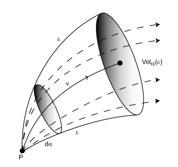
Figure S1: Schematic figure on the geometric interpretation of Ricci curvature. Ricci curvature quantifies the deviation of the manifold from being locally Euclidean in tangent directions. In a $n$-dimensional Riemannian manifold, Ricci curvature controls the growth of $(n-1)$-volume $\text{Vol}_{\alpha}(\epsilon)$ generated within an $n$-solid angle $\mathrm{d}\alpha$ by geodesics of length $\epsilon$ in the direction of the vector $v$. Ricci curvature also quantifies the dispersion rate of geodesics with the same initial point and contained within the given solid angle.

The classical notion of Ricci curvature applies to smooth manifolds, and its classical definition requires tensors and higher-order derivatives Jost (2017). Thus, the classical definition of Ricci curvature is not immediately applicable in the discrete context of graphs or networks. Therefore, in order to develop any meaningful notion of Ricci curvature for networks, one has to inspect the essential geometric properties captured by this curvature notion, and find their proper analogues for discrete networks. To this end, it is essential to recall that Ricci curvature quantifies two essential geometric properties of the manifold, namely, volume growth and dispersion of geodesics. See Electronic Supplementary Material (ESM) Figure S1 for a schematic illustration of the Ricci curvature. Further, since classical Ricci curvature is associated to a vector (direction) in smooth manifolds Jost (2017), in the discrete case of networks, it is naturally assigned to edges Samal et al. (2018). Thus, notions of discrete Ricci curvatures are associated to edges rather than vertices or nodes in networks Samal et al. (2018). Note that no discretization of Ricci curvature for networks can capture the full spectrum of properties of the classical Ricci curvature defined on smooth manifolds, and thus, each discretization can shed a different light on the analyzed networks Samal et al. (2018). In this work, we apply four notions of discrete Ricci curvature for networks to study the correlation-based networks of stock markets.

Ollivier-Ricci curvature

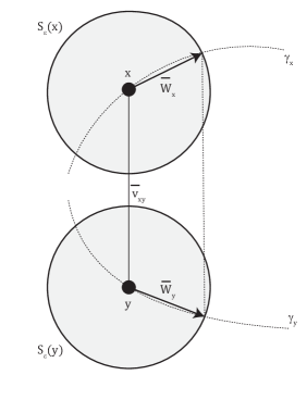
Figure S2: Schematic figure on the geometric interpretation of Ollivier-Ricci (OR) curvature. Consider two close points $x$ and $y$ in a $n$-dimensional Riemannian manifold, defining a tangent vector $\bar{v}_{xy}$. In Ollivier-Ricci curvature, one considers the parallel transport in the direction $\bar{v}_{xy}$ wherein points on a infinitesimal sphere $S_{\varepsilon}(x)$ centered at $x$, are transported to points on the corresponding sphere $S_{\varepsilon}(y)$. In spaces of positive (respectively, negative) Ricci curvature, balls are closer (respectively, farther) than their centers.

Ollivier’s discretization Ollivier (2007, 2009) of the classical Ricci curvature has been extensively used to analyze graphs or networks Lin and Yau (2010); Lin et al. (2011); Bauer et al. (2012); Jost and Liu (2014); Ni et al. (2015); Sandhu et al. (2015, 2016); Samal et al. (2018); Ni et al. (2019); Sia et al. (2019). Ollivier’s definition is based on the following observation. In spaces of positive curvature, balls are closer to each other on the average than their centers, while in spaces of negative curvature, balls are farther away on the average than their centers (ESM Figure S2). Ollivier’s definition extends this observation from balls (volumes) to measures (probabilities). More precisely, the Ollivier-Ricci (OR) curvature of an edge $e$ between nodes $u$ and $v$ is defined as

$$\mathbf{O}(e)=1-\frac{W_{1}(m_{u},m_{v})}{d(u,v)}\,$$ (1)

where $m_{u}$ and $m_{v}$ represent measures concentrated at nodes $u$ and $v$, respectively, $W_{1}$ denotes the Wasserstein distance Vaserstein (1969) (also known as the earth mover’s distance) between the discrete probability measures $m_{u}$ and $m_{v}$, and the cost $d(u,v)$ is the distance between nodes $u$ and $v$, respectively. Moreover, the Wasserstein distance $W_{1}(m_{u},m_{v})$ which gives the transportation distance between the two measures $m_{u}$ and $m_{v}$, is given by

$$W_{1}(m_{u},m_{v})=\inf_{\mu_{u,v}\in\prod(m_{u},m_{v})}\sum_{(u^{\prime},v^{\prime})\in V\times V}d(u^{\prime},v^{\prime})\mu_{u,v}(u^{\prime},v^{\prime}),$$ (2)

with $\prod(m_{u},m_{v})$ being the set of probability measures $\mu_{u,v}$ that satisfy

$$\sum_{v^{\prime}\in V}\mu_{u,v}(u^{\prime},v^{\prime})=m_{u}(u^{\prime}),\,\,\sum_{u^{\prime}\in V}\mu_{u,v}(u^{\prime},v^{\prime})=m_{v}(v^{\prime})$$ (3)

where $V$ is the set of nodes in the graph. The above equation represents all the transportation possibilities of the mass $m_{u}$ to $m_{v}$. $W_{1}(m_{u},m_{v})$ is the minimal cost or distance to transport the mass of $m_{u}$ to that of $m_{v}$. Note that the distance $d(u^{\prime},v^{\prime})$ in Eq. 2 is taken to be the path distance in the unweighted or weighted graph. Furthermore, the probability distribution $m_{u}$ for $u\in V$ has to be specified, and this is chosen to be uniform over neighbouring nodes of $u$ Lin et al. (2011).

Simply stated, to determine the OR curvature of an edge $e$, in Eq. 1 one compares the average distance between the neighbours of the nodes $u$ and $v$ anchoring the edge $e$ in an optimal arrangement with the distance between $u$ and $v$ itself. Importantly, the average distance between neighbours of $u$ and $v$ is evaluated as an optimal transport problem wherein the neighbours of $u$ are coupled with those of $v$ in such a manner that the average distance is as small as possible. In the setting of discrete graphs or networks, OR curvature by definition captures the volume growth aspect of the classical notion for smooth manifolds, see e.g. Samal et al. (2018) for details. In this work, we have computed the average OR curvature of edges (ORE) in undirected and weighted networks using Eq. 1.

Forman-Ricci curvature

Forman’s approach to the discretization of Ricci curvature Forman (2003) is more algebraic in nature and is based on the relation between the Riemannian Laplace operator and Ricci curvature. While devised originally for a much larger class of discrete geometric objects than graphs, an adaptation to network setting was recently introduced by some of us Sreejith et al. (2016). The Forman-Ricci (FR) curvature $\mathbf{F}(e)$ of an edge $e$ in an undirected network with weights assigned to both edges and nodes is given by Sreejith et al. (2016)

$$\mathbf{F}(e)=w_{e}\left(\frac{w_{v_{1}}}{w_{e}}+\frac{w_{v_{2}}}{w_{e}}-\sum_{e_{v_{1}}\ \sim\ e,\ e_{v_{2}}\ \sim\ e}\left[\frac{w_{v_{1}}}{\sqrt{w_{e}w_{e_{v_{1}}}}}+\frac{w_{v_{2}}}{\sqrt{w_{e}w_{e_{v_{2}}}}}\right]\right)\,$$ (4)

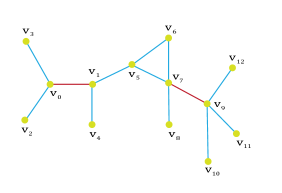
Figure S3: An illustrative example of the computation of the Forman-Ricci (FR) curvature of edges in a unweighted and undirected graph with 13 nodes and 13 edges. The FR curvature of an edge $e$ depends only on the weights of its neighbouring edges and the two nodes constituting the edge (see Eq. 2.4 in main text). In the simplest case of unweighted graphs, the weights of nodes and edges are equal to $1$, and thus, the FR curvature of an edge $e$ in such an undirected graph is given by $\mathbf{F}(e=(v_{i},v_{j}))=4-\text{degree}(v_{i})-\text{degree}(v_{j})$. In this example, the FR curvature of the edge $(v_{0},v_{1})$ depends only on the edges connected to nodes $v_{0}$ and $v_{1}$ with degree 3 and 3, respectively. Therefore, $\mathbf{F}(v_{0},v_{1})=4-3-3=-2$. Similarly, the FR curvature of the edge $(v_{7},v_{9})$ depends only on the edges connected to nodes $v_{7}$ and $v_{9}$ with degree 4 and 4, respectively. Therefore, $\mathbf{F}(v_{7},v_{9})=4-4-4=-4$. As the edge $(v_{7},v_{9})$ has higher information spread at its ends (or anchoring nodes) in comparison to the edge $(v_{0},v_{1})$, it has more negative value of FR curvature.

where $e$ denotes the edge under consideration between nodes $v_{1}$ and $v_{2}$, $w_{e}$ denotes the weight of the edge $e$, $w_{v_{1}}$ and $w_{v_{2}}$ denote the weights associated with the nodes $v_{1}$ and $v_{2}$, respectively, $e_{v_{1}}\sim e$ and $e_{v_{2}}\sim e$ denote the set of edges incident on nodes $v_{1}$ and $v_{2}$, respectively, after excluding the edge $e$ under consideration which connects the two nodes $v_{1}$ and $v_{2}$. Furthermore, some of us have also extended the notion of FR curvature to directed networks Saucan et al. (2019a). In case of discrete networks, FR curvature captures the geodesic dispersal property of the classical notion Samal et al. (2018). In ESM Figure S3, we illustrate, using a simple example, the computation of FR curvature in an undirected graph. In this work, we have computed the average FR curvature of edges (FRE) in undirected and weighted networks using Eq. 4.

From a geometric perspective, the FR curvature quantifies the information spread at the ends of edges in a network (Figure 1; ESM Figure S3). The higher the information spread at the ends of an edge, the more negative will be the value of its FR curvature. Specifically, an edge with high negative FR curvature is likely to have several neighbouring edges connected to both anchoring nodes, and moreover, such an edge can be seen as a funnel at both ends, connecting many other nodes. Intuitively, such an edge with high negative FR curvature can be expected to have high edge betweenness centrality as many shortest paths between other nodes, including those quite far in the network, are also likely to pass through this edge. Previously, some of us have empirically shown a high statistical correlation between FR curvature and edge betweenness centrality in diverse networks Sreejith et al. (2017); Samal et al. (2018).

Menger-Ricci curvature

The remaining two curvatures studied here are adaptations of curvatures for metric spaces to discrete graphs. Indeed, both unweighted and weighted graphs can be viewed as a metric space where the distance between any two nodes can be specified by the path length between them. Among notions of metric, and indeed, discrete curvature, Menger Menger (1930) has proposed the simplest and earliest definition whereby he defines the curvature of metric triangles $T$ formed by three points in the space as the reciprocal $1/R(T)$ of the radius $R(T)$ of the circumscribed circle of a triangle $T$. Recently, some of us Saucan et al. (2019b, 2020) have adapted Menger’s definition to networks. Let $(M,d)$ be a metric space and $T=T(a,b,c)$ be a triangle with sides $a,\ b,\ c$, then the Menger curvature of $T$ is given by

$$K_{M}(T)=\frac{\sqrt{p(p-a)(p-b)(p-c)}}{a\cdot b\cdot c}\,$$ (5)

where $p=(a+b+c)/2$. In the particular case of a combinatorial triangle with each side of length 1, the above formula gives $K_{M}(T)=\sqrt{3}/2$. Furthermore, it is clear from the above formula that Menger curvature is always positive. Following the differential geometric approach, the Menger-Ricci (MR) curvature of an edge $e$ in a network can be defined as Saucan et al. (2019b, 2020)

$$\kappa_{M}(e)=\sum_{T_{e}\sim e}\kappa_{M}(T_{e})\,,$$ (6)

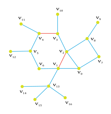
Figure S4: An illustrative example of the computation of the Menger-Ricci (MR) and Haantjes-Ricci (HR) curvature of edges in a unweighted and undirected graph with 17 nodes and 19 edges. The MR curvature of an edge $e$ depends only on the triangles adjacent to it (see Eq. 2.6 in main text), while the HR curvature depends on simple paths of any length that connect the two nodes at ends of the edge (see Eq. 2.9 in main text). In case of unweighted graphs, each triangle adjacent to an edge $e$ contributes $\sqrt{3}/2$ to its MR curvature. In case of unweighted graphs, each path of length $n$ between the two nodes at the ends of an edge $e$ contributes $\sqrt{n-1}$ to its HR curvature. In this example, for the edge $(v_{3},v_{4})$, the MR curvature is 0 as there are no triangles adajacent to the edge, while the HR curvature is $\sqrt{4}$ as there is only a path $\pi=v_{3},v_{2},v_{1},v_{6},v_{5},v_{4}$ of length 5 other than the edge connecting the nodes $v_{3}$ and $v_{4}$. For the edge $(v_{1},v_{2})$, the MR curvature is $\sqrt{3}/2$ as there is one triangle $v_{0},v_{1},v_{2}$ adjacent to the edge, while the HR curvature is $1+\sqrt{3}+\sqrt{4}$ as there is a path $v_{1},v_{0},v_{2}$ of length 2, a path $v_{1},v_{0},v_{7},v_{8},v_{2}$ of length 4, and a path $v_{1},v_{6},v_{5},v_{4},v_{3},v_{2}$ of length 5 other than the edge connecting the nodes $v_{1}$ and $v_{2}$. It can be seen from this simple example that HR curvature is more general than MR curvature as it depends on paths of any length unlike MR curvature which is dependent on only triangles.

where $T_{e}\sim e$ denote the triangles adjacent to the edge $e$. Intuitively, if an edge is part of several triangles in the network, such an edge will have high positive MR curvature (Figure 1). In ESM Figure S4, we illustrate, using a simple example, the computation of MR curvature in an undirected graph. In this work, we have computed the average MR curvature of edges (MRE) in undirected financial networks by ignoring the edge weights and using Eq. 6.

Haantjes-Ricci curvature

We have also applied another notion of metric curvature to networks which is based on the suggestion of Finsler and was developed by his student Haantjes Haantjes (1947). Haantjes defined the curvature of a metric curve as the ratio between the length of an arc of the curve and that of the chord it subtends. More precisely, given a curve $c$ in a metric space $(M,d)$, and given three points $p,q,r$ on $c$, $p$ between $q$ and $r$, the Haantjes curvature at the point $p$ is defined as

$$\kappa_{H}^{2}(p)=24\lim_{q,r\rightarrow p}\frac{l(\widehat{qr})-d(q,r)}{\big{(}d(q,r)\big{)}^{3}}\,,$$ (7)

where $l(\widehat{qr})$ denotes the length, in the intrinsic metric induced by $d$, of the arc $\widehat{qr}$. In networks, $\widehat{qr}$ can be replaced by a path $\pi=v_{0},v_{1},\ldots,v_{n}$ between two nodes $v_{0}$ and $v_{n}$, and the subtending chord by the edge $e=(v_{0},v_{n})$ between the two nodes. Recently, some of us Saucan et al. (2019b, 2020) have defined the Haantjes curvature of such a simple path $\pi$ as

$$\kappa_{H}^{2}(\pi)=\frac{l(\pi)-l(v_{0},v_{n})}{l(v_{0},v_{n})^{3}}\,,$$ (8)

where, if the graph is a metric graph, $l(v_{0},v_{n})=d(v_{0},v_{n})$, that is the shortest path distance between nodes $v_{0}$ and $v_{n}$. In particular, for the combinatorial metric (or unweighted graphs), we obtain that $\kappa_{H}(\pi)=\sqrt{n-1}$, where $\pi=v_{0},v_{1},\ldots,v_{n}$ is as above. Note that considering simple paths in graphs concords with the classical definition of Haantjes curvature, since a metric arc is, by its very definition, a simple curve. Thereafter, the Haantjes-Ricci (HR) curvature of an edge $e$ Saucan et al. (2019b, 2020) can be defined as

$$\kappa_{H}(e)=\sum_{\pi\sim e}\kappa_{H}(\pi)\,,$$ (9)

where $\pi\sim e$ denote the paths that connect the nodes anchoring the edge $e$. Note that while MR curvature considers only triangles or simple paths of length 2 between two nodes anchoring an edge in unweighted graphs, the HR curvature considers even longer paths between the same two nodes anchoring an edge (Figure 1). Moreover, for triangles endowed with the combinatorial metric, the two notions by Menger and Haantjes coincide, up to a universal constant. In ESM Figure S4, we illustrate, using a simple example, the computation of HR curvature in an undirected graph. In this work, we have computed the average HR curvature of edges (HRE) in undirected financial networks by ignoring the edge weights and using Eq. 9. Moreover, due to computational constraints, we only consider simple paths $\pi$ of length $\leq 4$ between the two vertices at the ends of any edge while computing its HR curvature using Eq. 9 in analyzed networks. Note that both Menger and Haantjes curvature are positive in undirected networks, and they capture the (absolute value of) geodesics dispersal rate of the classical Ricci curvature.

3 Data and Methods

Data description

The data was collected from the public domain of Yahoo finance database Yah for two markets: USA S&P-500 index and Japanese Nikkei-225 index. The investigation in this work spans a 32-year period from 2 January 1985 (02-01-1985) to 30 December 2016 (30-12-2016). We analyzed the daily closure price data of $N=194$ stocks for $T=8068$ days for USA S&P-500 and $N=165$ stocks for $T=7998$ days for Japanese Nikkei-225 markets. ESM Tables S1 and S2 give the lists of 194 and 165 stocks (along with their sectors) for the USA S&P-500 and Japanese Nikkei-225 markets, respectively, and these stocks are present in the two markets for the entire 32-year period considered here.

Cross-correlation and distance matrices

We present a study of time evolution of the cross-correlation structures of return time series for $N$ stocks (Figure 1). The daily return time series is constructed as $r_{k}(t)=\ln P_{k}(t)-\ln P_{k}(t-1)$, where $P_{k}(t)$ is the adjusted closing price of the $k^{\text{th}}$ stock at time $t$ (trading day). Then, the cross-correlation matrix is constructed using equal-time Pearson cross-correlation coefficients,

$$C_{ij}(t)=(\langle r_{i}r_{j}\rangle-\langle r_{i}\rangle\langle r_{j}\rangle)/\sigma_{i}\sigma_{j},$$

where $i,j=1,\dots,N$, $t$ indicates the end date of the epoch of size $\tau$ days, and the means $\langle\dots\rangle$ as well as the standard deviations $\sigma_{k}$ are computed over that epoch.

Instead of working with the correlation coefficient $C_{ij}(t)$, we use the ‘ultrametric’ distance measure:

$$D_{ij}(t)=\sqrt{2(1-C_{ij}(t))},$$

such that $0\leq D_{ij}(t)\leq 2$, which can be used for the construction of networks Mantegna (1999a, b); Onnela et al. (2003); Kumar and Deo (2012).

Here, we computed daily return cross-correlation matrix $\boldsymbol{C}_{\tau}(t)$ over the short epoch of $\tau=22$ days and shift of the rolling window by $\Delta\tau=5$ days, for (a) $N=194$ stocks of USA S&P-500 for a return series of $T=8068$ days, and (b) $N=165$ stocks of Japan Nikkei-225 for $T=7998$ days, during the 32-year period from 1985 to 2016. We use epochs of $\tau=22$ days (one trading month) to obtain a balance between choosing short epochs for detecting changes and long ones for reducing fluctuations. In the main text, we show results for networks constructed from correlation matrices with overlapping windows of $\Delta\tau=5$ days, while in ESM, we show results for networks constructed from correlation matrices with non-overlapping windows of $\Delta\tau=22$ days.

Network construction

For a given time window of $\tau$ days ending on trading day $t$, the distance matrix $\boldsymbol{D}_{\tau}(t)$ constructed from the correlation matrix between the 194 stocks in USA S&P-500 index or the 165 stocks in Japan Nikkei-225 index, can be viewed as an undirected complete graph $G_{\tau}(t)$ where the weight of an edge between stocks $i$ and $j$ is given by the distance $D_{ij}(t)$. For the time window of $\tau$ days ending on trading day $t$, we start with this edge weighted complete graph $G_{\tau}(t)$ and create the minimum spanning tree (MST) $T_{\tau}(t)$ using Prim’s algorithm Prim (1957). Thereafter, we add edges in $G_{\tau}(t)$ with $C_{ij}(t)\geq 0.75$ to $T_{\tau}(t)$ to obtain the graph $S_{\tau}(t)$ (Figure 1). We will use the graph $S_{\tau}(t)$ to compute different discrete Ricci curvatures and other network measures. We remark that the procedure used here to construct the graph $S_{\tau}(t)$ follows previous works Onnela et al. (2003); Sandhu et al. (2016) on analysis of correlation-based networks of stock markets.

Intuitively, the motivation behind the above method of graph construction can be understood as follows. Firstly, the MST method gives a connected (spanning) graph between all nodes (stocks) in the specific market. Secondly, the addition of edges between nodes (stocks) with correlation $C_{ij}(t)\geq 0.75$ ensures that the important edges are also captured in the graph $S_{\tau}(t)$.

Common network measures

Given an undirected graph $G(V,E)$ with the sets of vertices or nodes $V$ and edges $E$, the number of edges is given by the cardinality of set $E$, that is $m=|E|$, and the number of nodes is given by the cardinality of set $V$, that is $n=|V|$. The edge density of such a graph is given by the ratio of the number of edges $m$ divided by the number of possible edges, that is, $\frac{2m}{n(n-1)}$. The average degree $\langle k\rangle$ of the graph gives the average number of edges per node, that is, $\langle k\rangle=\frac{m}{n}$. In case of an edge-weighted graph where $a_{ij}$ denotes the weight of the edge between nodes $i$ and $j$, one can also compute its average weighted degree $\langle k_{w}\rangle$ which gives the average of the sum of the weights of the edges connected to nodes, that is, $\langle k_{w}\rangle=\frac{m_{w}}{n}$ where $m_{w}=\sum_{i,j\in V}a_{ij}$. For any pair of nodes $i$ and $j$ in the graph, one can compute the shortest path length $d_{ij}$ between them. Thereafer, the average shortest path length $\langle L\rangle$ is given by the average of the shortest path lengths between all pairs of nodes in the graph, that is,

$$\langle L\rangle=\frac{1}{n(n-1)}\sum_{i\neq j\in V}d_{ij}.$$

The diameter is given by the maximum of the shortest paths between all pairs of nodes in the graph, i.e., $\text{max}\{d_{ij}\ \forall i,j\in V\}$. The communication efficiency Latora and Marchiori (2001) of a graph is an indicator of its global ability to exchange information across the network. The communication efficiency $CE$ of a graph is given by

$$CE=\frac{1}{n(n-1)}\sum_{i\neq j\in V}\frac{1}{d_{ij}}.$$

Modularity measures the extent of community structure in the network and community detection algorithms aim to partition the graph into communities such that the modularity $Q$ attains the maximum value Girvan and Newman (2002). The modularity $Q$ is given by the equation Girvan and Newman (2002); Blondel et al. (2008)

$$Q=\frac{1}{2m_{w}}\sum_{i\neq j\in V}[\,a_{ij}-\frac{k_{i}k_{j}}{2m_{w}}]\delta(c_{i},c_{j})\,$$

where $k_{i}$ and $k_{j}$ give the sum of weights of edges attached to nodes $i$ and $j$, respectively, $c_{i}$ and $c_{j}$ give the communities of $i$ and $j$, respectively, and $\delta(c_{i},c_{j})$ is equal to 1 if $c_{i}=c_{j}$ else 0. Here, we use Louvain method Blondel et al. (2008) to compute the modularity of the edge-weighted networks. Network entropy is an average measure of graph heterogeneity as it quantifies the diversity of edge distribution using the remaining degree distribution $q_{k}$ Solé and Valverde (2004). $q_{k}$ denotes the probabibility of a node to have remaining (excess) degree $k$ and is given by $q_{k}=\frac{(k+1)p_{k+1}}{<k>}$ where $p_{k+1}$ denotes the probability of a node to have degree $k+1$. The network entropy $H(q)$ of a graph is then given by

$$H(q)=-\sum_{k}q_{k}log(q_{k}).$$

The above-mentioned network measures were computed in stock market networks using the python package NetworkX Hagberg et al. (2008).

GARCH($p,q$) process

The generalized ARCH process GARCH($p,q$) was introduced by Bollerslev Bollerslev (1986). The variable $x_{t}$, a strong white noise process, can be written in terms of a time-dependent standard deviation $\sigma_{t}$, such that $x_{t}\equiv\eta_{t}\sigma_{t}$, where $\eta_{t}$ is a random Gaussian process with zero mean and unit variance.

The simplest GARCH process is the GARCH(1,1) process, with Gaussian conditional probability distribution function

$$\sigma_{t}^{2}=\alpha_{0}+\alpha_{1}x_{t-1}^{2}+\beta_{1}\sigma_{t-1}^{2}\,,$$ (10)

where $\alpha_{0}>0$ and $\alpha_{1}\geq 0$; $\beta_{1}$ is an additional control parameter. One can rewrite Eq. 10 as a random multiplicative process

$$\sigma_{t}^{2}=\alpha_{0}+(\alpha_{1}\eta_{t-1}^{2}+\beta_{1})\sigma_{t-1}^{2}\,.$$ (11)

For calculating this we have used an in-built function from MATLAB garch (https://in.mathworks.com/help/econ/garch.html).

Minimum Risk Portfolio

We calculated the minimum risk portfolio in the Markowitz framework, as a measure of risk-aversion of each investor with maximized expected returns and minimized variance. In this model, the variance of a portfolio shows the importance of effective diversification of investments to minimize the total risk of a portfolio. The Markowitz model minimizes $\mathrm{w}^{\prime}\Omega\mathrm{w}-\phi R^{\prime}\mathrm{w}$ with respect to the normalized weight vector $\mathrm{w}$, where $\Omega$ is the covariance matrix calculated from the stock log-returns, $\phi$ is the measure of risk appetite of investor and $R^{\prime}$ is the expected return of the assets. We set short-selling constraint, $\phi=0$ and $\mathrm{w}_{i}\geq 0$ which entails a convex combination of stock return for finding the minimum risk portfolio. For calculating this we have used an in-built function from MATLAB Portfolio (https://in.mathworks.com/help/finance/portfolio.html).

4 Results and Discussion

We analyze here the time series of the logarithmic returns of the stocks in the USA S&P-500 and Japanese Nikkei-225 markets over a period of 32 years (1985-2016) by constructing the corresponding Pearson cross-correlation matrices $\boldsymbol{C}_{\tau}(t)$. We then use cross-correlation matrices $\boldsymbol{C}_{\tau}(t)$ computed over time epochs of size $\tau=22$ days with either overlapping or non-overlapping windows (i.e. shifts of $\Delta\tau=5$ or $22$ days, respectively) and ending on trading days $t$ to study the evolution of the correlation-based networks $S_{\tau}(t)$ and corresponding network properties, especially edge-centric geometric measures. Figure 1 gives an overview of our evaluation of discrete Ricci curvatures in correlation-based threshold networks constructed from log-returns of market stocks. Figure 1(a) shows the daily log-returns over the 32-year period (1985-2016). An arbitrarily chosen cross-correlation matrix $\boldsymbol{C}_{\tau}(t)$ over time epoch of $\tau=22$ days and $\Delta\tau=5$ days ending on 04-05-2011 and corresponding distance matrix $\boldsymbol{D}_{\tau}(t)=\sqrt{2(1-\boldsymbol{C}_{\tau}(t))}$ are shown in Figure 1(b) and (c), respectively. The minimum spanning tree (MST) $T_{\tau}(t)$ constructed from the distance matrix $D_{\tau}(t)$ is shown in Figure 1(d). Thereafter, a threshold network $S_{\tau}(t)$ is constructed using MST $T_{\tau}(t)$ and edges with $C_{ij}(t)\geq 0.75$, as shown in Figure 1(e). The discrete Ricci curvatures are computed from the threshold networks. In Figure 1(f), we show the evolution of the discrete curvatures in threshold networks over the 32-year period. In Figure 1(g), we motivate the four discrete Ricci curvatures considered here using a simple example network.

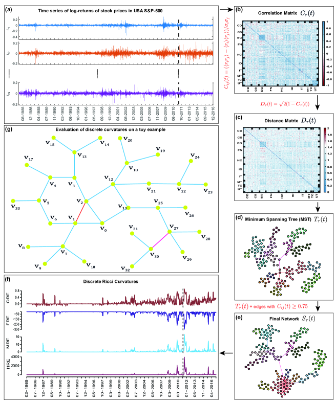
Figure 1: Schematic diagram describing the evaluation of discrete Ricci curvatures in correlation-based networks constructed from log-returns of USA S&P-500 market stocks. (a) Time series of log-returns over a 32-year period (1985-2016). (b) An arbitrarily chosen cross-correlation matrix $\boldsymbol{C}_{\tau}(t)$ for epoch ending on 04-05-2011. (c) Corresponding distance matrix $\boldsymbol{D}_{\tau}(t)=\sqrt{2(1-\boldsymbol{C}_{\tau}(t))}$ used for the construction of the threshold network. (d) Minimum spanning tree (MST) $T_{\tau}(t)$ constructed using the distance matrix $D_{\tau}(t)$. (e) Threshold network $S_{\tau}(t)$ constructed by adding edges with $C_{ij}(t)\geq 0.75$ to the MST $T_{\tau}(t)$. (f) Evolution of the average of four discrete Ricci curvatures for edges, namely, Ollivier-Ricci (ORE), Forman-Ricci (FRE), Menger-Ricci (MRE) and Haantjes-Ricci (HRE), computed using the threshold networks $S_{\tau}(t)$ constructed from correlation matrices over time epochs of $\tau=22$ days and overlapping shift of $\Delta\tau=5$ days. In this figure, $C_{\tau}(t)$, $D_{\tau}(t)$, $T_{\tau}(t)$ and $S_{\tau}(t)$ shown in (b)-(e) correspond to the correlation frame denoted by vertical dashed line in (a). (g) Evaluation of discrete Ricci curvatures on a toy example network which is undirected and unweighted. Here, the edge between $v_{27}$ and $v_{30}$ has a highly negative FR curvature as it depends on the degree of the two nodes or number of neighbouring edges. However, the edge between $v_{27}$ and $v_{30}$ has MR and HR curvature equal to zero as the edge under consideration is not part of any triangles or cycles, respectively. Moreover, the edge between $v_{1}$ and $v_{2}$ also has a highly negative FR curvature as the degree of both anchoring vertices is 4. In contrast, the edge between $v_{1}$ and $v_{2}$ has positive MR and HR curvature as the edge is part of a triangle which contributes to MR curvature and the edge is part of a triangle, a pentagon and a hexagon which contribute to HR curvature. For both the edges between $v_{27}$ and $v_{30}$ and between $v_{1}$ and $v_{2}$, one can compute OR curvature, however, only triangles, quadrangles and pentagons make positive contribution to the OR curvature in unweighted and undirected networks. Specifically, the edge between $v_{1}$ and $v_{2}$ is part of a triangle, a pentagon and a hexagon, however, only the triangle and pentagon make positive contribution to OR curvature.

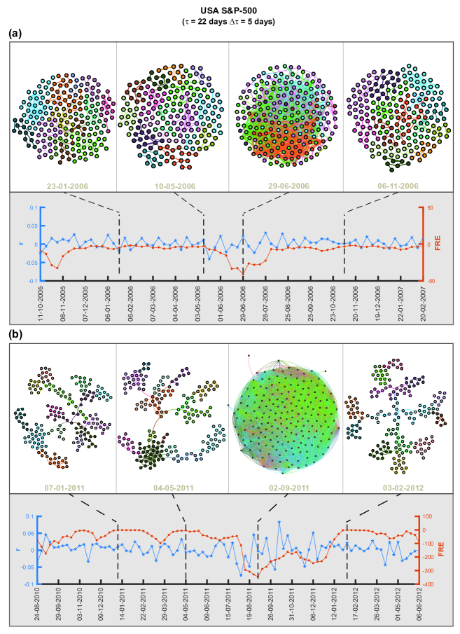
Figure 2: (a) (Upper panel) Visualization of threshold networks for USA S&P-500 market around the US Housing bubble period (2006-2007) at four distinct epochs of $\tau=22$ days ending on trading days 23-01-2006, 10-05-2006, 29-06-2006, and 06-11-2006, with threshold $C_{ij}(t)\geq 0.75$. Here, the colour of the nodes correspond to the different communities determined by Louvain method for community detection. Threshold networks show higher number of edges and lower number of communities during a bubble. (Lower panel) Plot shows the evolution of log-returns $r$ of S&P-500 index (blue color line) and average Forman-Ricci curvature of edges (FRE) (sienna color line) for the period around the US Housing bubble. The FRE measure, constructed from threshold networks, is sensitive to both local (sectoral) and global fluctuations of the market, and shows a local minimum (more negative) during the bubble, whereas not much variation is seen in $r$ (low volatility). (b) (Upper panel) Visualization of threshold networks for USA S&P-500 market around the August 2011 stock markets fall at four distinct epochs of $\tau=22$ days ending on 07-01-2011, 04-05-2011, 02-09-2011, and 03-02-2012 with threshold $C_{ij}(t)\geq 0.75$. Here, the threshold network shows significantly higher number of edges and lower number of communities during the crash. (Lower panel) Plot shows the evolution of log-returns $r$ of S&P 500 index (blue color line) and FRE (sienna color line) for the period around the August 2011 stock markets fall. During the crash $r$ has high fluctuations (high volatility) and FRE decreases significantly (local minima).

A major goal of this research is to evaluate different notions of discrete Ricci curvature for their ability to unravel the structure of complex financial networks and serve as indicators of market instabilities. Previously, Sandhu et al. Sandhu et al. (2016) have analyzed the USA S&P-500 market over a period of 15 years (1998-2013) to show that the average Ollivier-Ricci (OR) curvature of edges (ORE) in threshold networks increases during periods of financial crisis. Here, we extend the analysis by Sandhu et al. Sandhu et al. (2016) to (a) two different stock markets, namely, USA S&P-500 and Japanese Nikkei-225, (b) a span of 32 years (1985-2016), (c) four traditional market indicators (namely, index log-returns $r$, mean market correlation $\mu$, volatility of the market index $r$ estimated using GARCH(1,1) process, and risk $\sigma_{P}$ corresponding to the minimum risk Markowitz portfolio of all the stocks in the market), and (d) four notions of discrete Ricci curvature for networks. Since discretizations of Ricci curvature are unable to capture the entire properties of the classical Ricci curvature defined on continuous spaces, the four discrete Ricci curvatures evaluated here can shed light on different properties of analyzed networks Samal et al. (2018). In particular, some of us have introduced another discretization, Forman-Ricci (FR) curvature, to the domain of networks Sreejith et al. (2016). Note that OR curvature captures the volume growth property of classical Ricci curvature while FR curvature captures the geodesic dispersal property Samal et al. (2018). Nevertheless, our empirical analysis has shown that the two discrete notions, OR and FR curvature, are highly correlated in model and real-world networks Samal et al. (2018). Importantly, in large networks, computation of the OR curvature is intensive while that of the FR curvature is simple as the later depends only on immediate neighbours of an edge Samal et al. (2018). Therefore, we started by investigating the ability of FR curvature to capture the structure of complex financial networks.

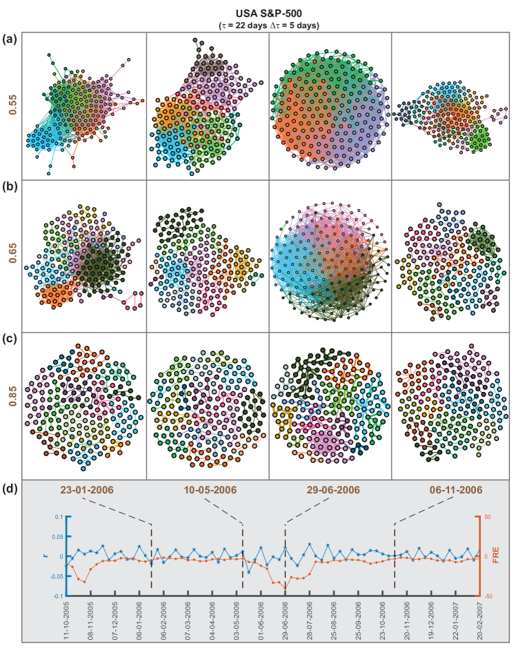
Figure S5: Visualization of threshold networks for USA S&P-500 market around the US Housing bubble period (2006-2007) at four distinct epochs of $\tau=22$ days ending on trading days 23-01-2006, 10-05-2006, 29-06-2006, and 06-11-2006, with thresholds (a) $C_{ij(t)}\geq 0.55$, (b) $C_{ij}(t)\geq 0.65$, and (c) $C_{ij}(t)\geq 0.85$. Here, the colour of the nodes correspond to the different communities determined by Louvain method for community detection. The number of edges and communities in $S_{\tau}(t)$ for different thresholds are shown in Table S3. (d) Plot shows the evolution of log-returns $r$ of S&P-500 index (blue color line) and average Forman-Ricci curvature of edges (FRE) (sienna color line) computed using threshold networks with $C_{ij}(t)\geq 0.75$ for the period around the US Housing bubble.

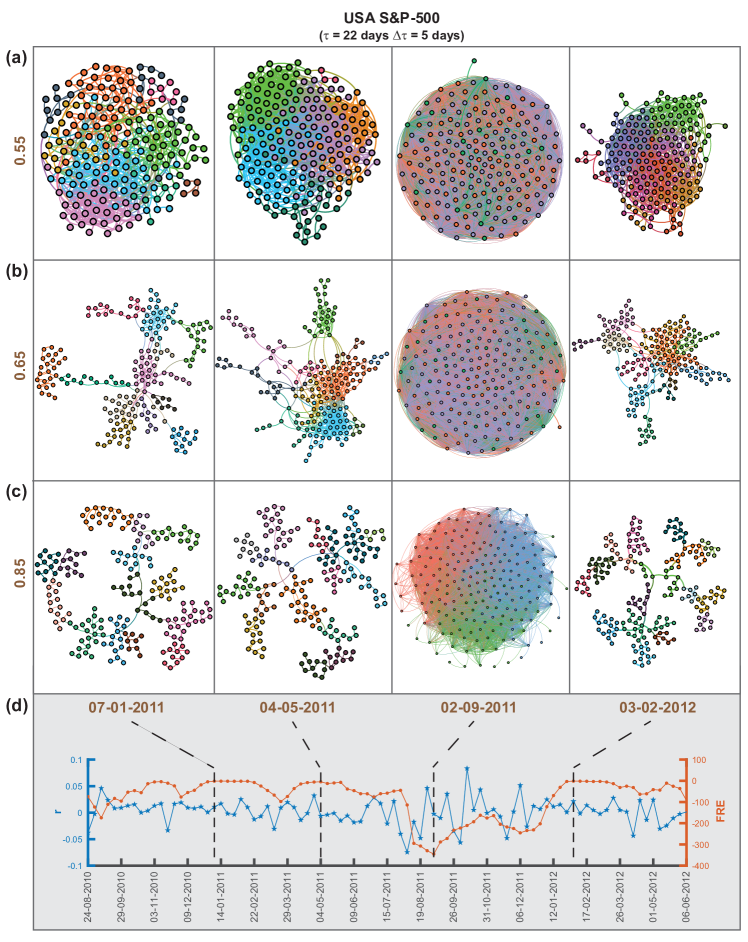
Figure S6: Visualization of threshold networks for USA S&P-500 market around the August 2011 stock markets fall at four distinct epochs of $\tau=22$ days ending on 07-01-2011, 04-05-2011, 02-09-2011, and 03-02-2012 with thresholds (a) $C_{ij}(t)\geq 0.55$, (b) $C_{ij}(t)\geq 0.65$, and (c) $C_{ij}(t)\geq 0.85$. Here, the colour of the nodes correspond to the different communities determined by Louvain method for community detection. The number of edges and communities in $S_{\tau}(t)$ for different thresholds are shown in Table S3. (d) Plot shows the evolution of log-returns $r$ of S&P-500 index (blue color line) and average Forman-Ricci curvature of edges (FRE) (sienna color line) computed using threshold networks with $C_{ij}(t)\geq 0.75$ for the period around the August 2011 stock markets fall crisis.

Figure 2 shows the comparisons of threshold networks, as well as the behaviour of index log-returns $r$ and average FR curvature of edges (FRE), for (a) bubble and (b) crash periods, of the USA S&P-500 market. The upper panel of Figure 2(a) shows the threshold networks near the US Housing bubble period (2006-2007) at four distinct epochs of $\tau=22$ days ending on trading days $t$ equal to 23-01-2006, 10-05-2006, 29-06-2006 and 06-11-2006, with threshold $C_{ij}(t)\geq 0.75$. Number of edges and communities in these four threshold networks are $251,220,996,220$ and $13,16,11,14$, respectively. The colour of the nodes correspond to the different communities determined by Louvain method Blondel et al. (2008) for community detection. The plots of log-returns of S&P-500 index $r$ (blue color line) and FRE (sienna color line) around the US Housing bubble period are shown in the lower panel of Figure 2(a). Threshold networks show higher number ($996$) of edges and lower number ($11$) of communities for high (negative) values of FRE, but there is not much variation of $r$. In ESM Figure S5, we show that the FRE captures the same features for three other thresholds $C_{ij}(t)\geq 0.55$, $C_{ij}(t)\geq 0.65$, and $C_{ij}(t)\geq 0.85$, and the numbers of edges and communities for each threshold is listed in ESM Table S3. The measure FRE is sensitive to both local (sectoral) and global (market) fluctuations, and shows a local minimum during bubble. Note that during a bubble, only a few sectors of the market perform well compared to the others (the stocks within the well-performing sectors are highly correlated, but the inter-sectoral correlations are low). It is hard to identify bubble by only monitoring the market index as the returns do not show much volatility. Figure 2(b) shows the same for the period around the August 2011 stock markets fall at four distinct epochs of $\tau=22$ days ending on trading days $t$ equal to 07-01-2011, 04-05-2011, 02-09-2011 and 03-02-2012, with threshold $C_{ij}(t)\geq 0.75$. Number of edges and communities in these four threshold networks are $197,245,16004,198$ and $14,16,4,15$, respectively. During the crash, the threshold network shows sufficiently higher number of edges and extremely low number of communities. In ESM Figure S6, we show that the FRE captures the same features for three other thresholds $C_{ij}(t)\geq 0.55$, $C_{ij}(t)\geq 0.65$, and $C_{ij}(t)\geq 0.85$, and the numbers of edges and communities for each threshold is listed in ESM Table S3. The plots of log-returns $r$ of S&P-500 index (blue color line) and FRE (sienna color line) are shown around the August 2011 stock markets fall period in the lower panel of Figure 2(b). Note that during a market crash $r$ displays high volatility and FRE shows a significant decrease (local minimum). Earlier Sandhu et al. Sandhu et al. (2016) had focussed on OR curvature as an indicator of crashes. Here, we additionally show that discrete Ricci curvatures, especially FR curvature, are sensitive and can detect both crash (market volatility high) and bubble (market volatility low).

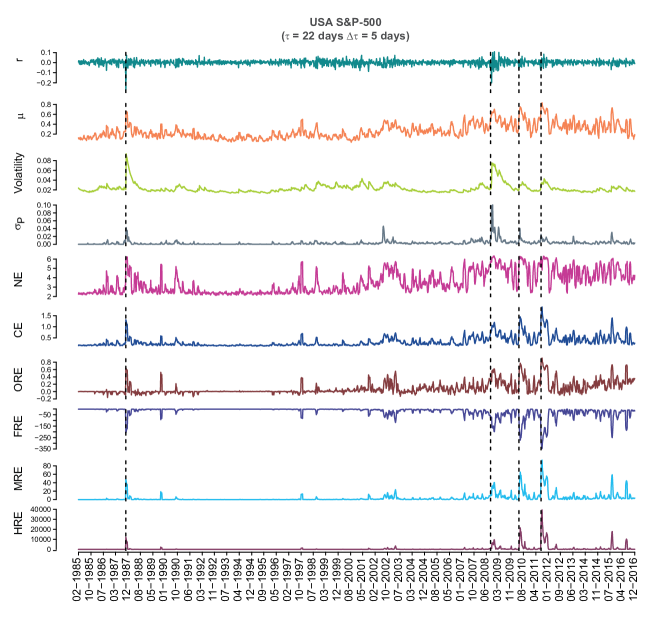
Figure 3: Evolution of the market indicators and edge-centric geometric curvatures for the USA S&P-500 market. From top to bottom, we plot the index log-returns $r$, mean market correlation $\mu$, volatility of the market index $r$ estimated using GARCH(1,1) process, risk $\sigma_{P}$ corresponding to the minimum risk Markowitz portfolio of all the stocks in the market, network entropy (NE), communication efficiency (CE), average of Ollivier-Ricci (ORE), Forman-Ricci (FRE), Menger-Ricci (MRE), and Haantjes-Ricci (HRE) curvature of edges evaluated from the correlation matrices $\boldsymbol{C}_{\tau}(t)$ of window size $\tau=22$ days and an overlapping shift of $\Delta\tau=5$ days. Four vertical dashed lines indicate the epochs of four important crashes: Black Monday 1987, Lehman Brothers crash 2008, DJ Flash crash 2010, and August 2011 stock markets fall (see Table 1).

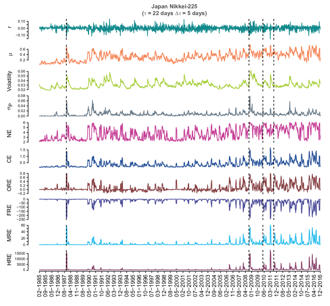
Figure 4: Evolution of the market indicators and edge-centric geometric curvatures for the Japanese Nikkei-225 market. From top to bottom, we plot the index log-returns $r$, mean market correlation $\mu$, volatility of the market index $r$ estimated using GARCH(1,1) process, risk $\sigma_{P}$ corresponding to the minimum risk Markowitz portfolio of all the stocks in the market, network entropy (NE), communication efficiency (CE), average of Ollivier-Ricci (ORE), Forman-Ricci (FRE), Menger-Ricci (MRE), and Haantjes-Ricci (HRE) curvature of edges evaluated from the correlation matrices $\boldsymbol{C}_{\tau}(t)$ of window size $\tau=22$ days and an overlapping shift of $\Delta\tau=5$ days. Four vertical dashed lines indicate the epochs of four important crashes: Black Monday 1987, Lehman Brothers crash 2008, DJ Flash crash 2010, and August 2011 stock markets fall (see Table 1).

It is often difficult to gauge the state of the market by simply monitoring the market index or its log-returns. There exist no simple definitions of a market crash or a market bubble. The market becomes extremely correlated and volatile during a crash, but a bubble is even harder to detect as the volatility is relatively low and only certain sectors perform very well (stocks show high correlation) but the rest of the market behaves like normal or ‘business-as-usual’. Traditionally, the volatility of the market captures the ‘fear’ and the evaluated risk captures the ‘fragility’ of the market. Some of us showed in our earlier papers that the mean market correlation and the spectral properties of the cross-correlation matrices can be used to study the market states Pharasi et al. (2018) and identify the precursors of market instabilities Chakraborti et al. (2020a). A goal of this study is to show that the state of the market can be continuously monitored with certain network-based measures. Thus, we next performed a comparative investigation of several network measures, especially, the four discrete notions of Ricci curvature.

Figures 3 and 4 show for USA S&P-500 market and Japanese Nikkei-225 market, respectively, the temporal evolution of the market indicators and network measures, mainly edge-centric Ricci curvatures computed from the correlation matrices $\boldsymbol{C}_{\tau}(t)$ of epoch size $\tau=22$ days and overlapping shift of $\Delta\tau=5$ days, over a 32-year period (1985-2016). From top to bottom, the plots represent index log-returns $r$, mean market correlation $\mu$, volatility of the market index $r$ estimated using GARCH(1,1) process, risk $\sigma_{P}$ corresponding to the minimum risk Markowitz portfolio of all the stocks in the market, network entropy (NP), communication efficiency (CE), average of OR, FR, MR and HR curvature of edges. We find that the four Ricci-type curvatures, namely, ORE, FRE, MRE and HRE, along with the other important indicators of the markets, viz., the log-returns $r$, volatility, minimum risk $\sigma_{P}$ and mean market correlation $\mu$, are excellent indicators of market instabilities (bubbles and crashes). We highlight that the four discrete Ricci curvatures can capture important crashes and bubbles listed in Table 1 in the two markets during the 32-year period studied here.

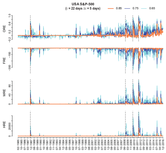
(a)

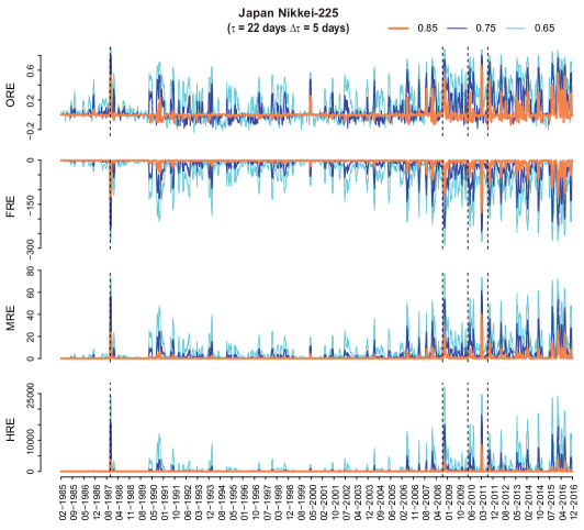
(b)

Figure S7: Comparison plots for the four edge-centric geometric curvatures, namely, Ollivier-Ricci (ORE), Forman-Ricci (FRE), Menger-Ricci (MRE) and Haantjes-Ricci (HRE) in threshold networks $S_{\tau}(t)$ obtained using three different thresholds $C_{ij}(t)\geq 0.65$ (cyan color), $C_{ij}(t)\geq 0.75$ (dark blue color), and $C_{ij}(t)\geq 0.85$ (sienna color) for (a) USA S&P-500 and (b) Japan Nikkei-225 markets. The curvature measures are calculated for time epochs of $\tau=22$ days and overlapping shift of $\Delta\tau=5$ days over the period (1985-2016). The absolute value of ORE, FRE, MRE and HRE decreases with the increase in the threshold $C_{ij}(t)$ used to construct $S_{\tau}(t)$. Four vertical dashed lines correspond to the epochs of four important crashes (Black Monday 1987, Lehman Brothers crash 2008, DJ Flash crash 2010, and August 2011 stock markets fall) listed in the Table 1 of the main text.

In ESM Figure S7, we show the temporal evolution of the four discrete Ricci curvatures computed in threshold networks $S_{\tau}(t)$ obtained using three different thresholds, $C_{ij}(t)\geq 0.65$ (cyan color), $C_{ij}(t)\geq 0.75$ (dark blue color) and $C_{ij}(t)\geq 0.85$ (sienna color), for the two markets. It is seen that the absolute value of ORE, FRE, MRE and HRE decreases with the increase in the threshold $C_{ij}(t)$ used to construct $S_{\tau}(t)$. Regardless of the three thresholds used to construct the threshold networks $S_{\tau}(t)$, we show that the four discrete Ricci curvatures are fine indicators of market instabilities.

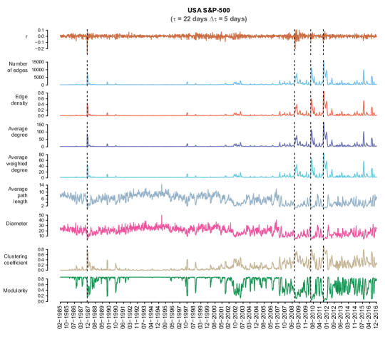
(a)

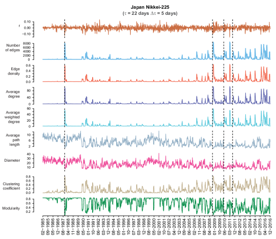
(b)

Figure S8: Evolution of network properties for (a) USA S&P-500 and (b) Japanese Nikkei-225 markets evaluated from the correlation matrices $\boldsymbol{C}_{\tau}(t)$ of window size $\tau=22$ days and an overlapping shift of $\Delta\tau=5$ days over the period (1985-2016). From top to bottom, we compare the plot of index log-returns $r$ with common network measures, namely, number of edges, edge density, average degree, average weighted degree, average path length, diameter, clustering coefficient and modularity.

In previous work, Sandhu et al. Sandhu et al. (2016) had contrasted the temporal evolution of ORE in threshold networks for USA S&P-500 market with NE, graph diameter and average shortest path length. Here, we have studied the temporal evolution of a larger set of network measures in threshold networks for USA S&P-500 and Japanese Nikkei-225 markets computed from the correlation matrices $\boldsymbol{C}_{\tau}(t)$ of epoch size $\tau=22$ days and overlapping shift of $\Delta\tau=5$ days, over a 32-year period (1985-2016). From Figures 3 and 4, it is seen that NE and CE are also excellent indicators of market instabilities. In fact, we find that common network measures such as number of edges, edge density, average degree, average shortest path length, graph diameter, average clustering coefficient and modularity are also good indicators of market instabilities (ESM Figure S8).

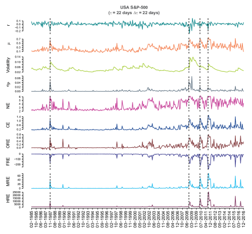
(a)

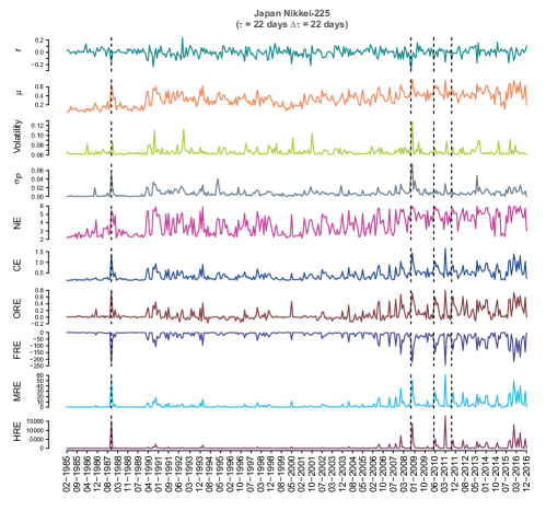
(b)

Figure S9: Evolution of the market indicators and edge-centric geometric curvatures for (a) USA S&P-500 and (b) Japanese Nikkei-225 markets. From top to bottom, we plot the index log-returns $r$, mean market correlation $\mu$, volatility of the market index $r$ estimated using GARCH(1,1) process, risk $\sigma_{P}$ corresponding to the minimum risk Markowitz portfolio of all the stocks in the market, network entropy (NE), communication efficiency (CE), average of Ollivier-Ricci (ORE), Forman-Ricci (FRE), Menger-Ricci (MRE), and Haantjes-Ricci (HRE) curvature of edges evaluated from the correlation matrices $\boldsymbol{C}_{\tau}(t)$ of window size $\tau=22$ days and a non-overlapping shift of $\Delta\tau=22$ days. Four vertical dashed lines indicate the epochs of four important crashes: Black Monday 1987, Lehman Brothers crash 2008, DJ Flash crash 2010, and August 2011 stock markets fall.

In ESM Figures S9 and S10, we show the temporal evolution of the market indicators and several network measures (including edge-centric Ricci curvatures) computed from the correlation matrices $\boldsymbol{C}_{\tau}(t)$ of epoch size $\tau=22$ days and non-overlapping shift of $\Delta\tau=22$ days, over a 32-year period (1985-2016) in the two markets. It can be seen that our results are also not dependent on the choice of overlapping or non-overlapping shift used to construct the cross-correlation matrices and threshold networks.

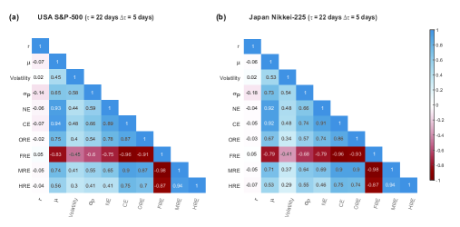
Figure 5: Correlogram plots of (a) USA S&P-500 and (b) Japan Nikkei-225 markets, for the traditional market indicators (index returns $r$, mean market correlation $\mu$, volatility, and minimum risk portfolio $\sigma_{P}$), global network properties (network entropy NE and communication efficiency CE) and discrete Ricci curvatures for edges (Ollivier-Ricci ORE, Forman-Ricci FRE, Menger-Ricci MRE, and Haantjes-Ricci HRE), computed for epochs of size $\tau=22$ days and overlapping shift $\Delta\tau=5$ days.

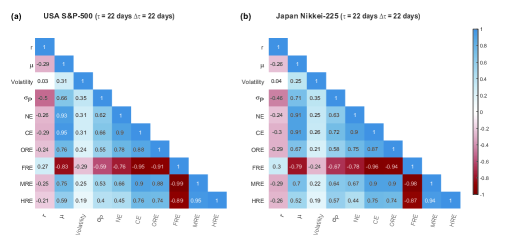
Figure S11: Correlogram plots of (a) USA S&P-500 and (b) Japan Nikkei-225 markets, for the traditional market indicators (index returns $r$, mean market correlation $\mu$, volatility, and minimum portfolio risk $\sigma_{P}$), network properties (network entropy (NE) and communication efficiency (CE)) and discrete Ricci curvatures for edges (Ollivier-Ricci ORE, Forman-Ricci FRE, Menger-Ricci MRE, and Haantjes-Ricci HRE), computed for epochs of size $\tau=22$ days and non-overlapping shift of $\Delta\tau=22$ days. Among the four curvature measures, FRE has the highest correlation with the market indicators, and this measure can be used as an indicator of market risk as it captures local to global system-level fragility of the markets.

Figure 5 shows the correlogram plots of (a) USA S&P-500 and (b) Japanese Nikkei-225 markets, for the traditional market indicators (index returns $r$, mean market correlation $\mu$, volatility, and minimum portfolio risk $\sigma_{P}$), network properties (NE and CE) and discrete Ricci curvatures (ORE, FRE, MRE and HRE), computed for epoch size $\tau=22$ days and overlapping shift of $\Delta\tau=5$ days. In ESM Figure S11, we show the correlogram plots for the traditional market indicators and network properties including discrete Ricci curvatures computed for epoch size $\tau=22$ days and non-overlapping shift of $\Delta\tau=22$ days in the two markets. Notably, FRE shows the highest correlation among the four discrete Ricci curvatures with the four traditional market indicators in the two markets, and thus, FRE is an excellent indicator for market risk that captures local to global system-level fragility of the markets. Furthermore, both NE and CE also have high correlation with the four traditional market indicators. Therefore, these measures can be used to monitor the health of the financial system and forecast market crashes or downturns. Overall, we show that FRE is a simple yet powerful tool for capturing the correlation structure of a dynamically changing network.

Table 1: List of major crashes and bubbles in stock markets of USA and Japan between 1985-2016 Cra (a); Bul ; USh ; Cra (b); Sel ; mar .

Serial number	Major crashes and bubbles	Period	Affected region
1	Black Monday	19-10-1987	USA, Japan
2	Friday the $13^{th}$ mini crash	13-10-1989	USA
3	Early 90s recession	1990	USA
4	Mini crash due to Asian financial crisis	27-10-1997	USA
5	Lost decade	2001-2010	Japan
6	9/11 financial crisis	11-09-2001	USA, Japan
7	Stock market downturn of 2002	09-10-2002	USA, Japan
8	US Housing bubble	2005-2007	USA
9	Lehman Brothers crash	16-09-2008	USA, Japan
10	Dow Jones (DJ) Flash crash	06-05-2010	USA, Japan
11	Tsunami and Fukushima disaster	11-03-2011	Japan
12	August 2011 stock markets fall	08-08-2011	USA, Japan
13	Chinese Black Monday and 2015-2016 sell off	24-08-2015	USA

5 Conclusion

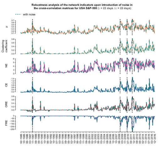
Figure S12: Evolution of network properties for USA S&P-500 market, evaluated from the empirical correlation matrices $C_{\tau}(t)$ and the correlation matrices perturbed by small amounts of random Gaussian noise (off diagonal elements of Wishart matrix with dimension same as $C_{\tau}(t)$), keeping correlation coefficients bounded in the range $[-1,1]$, for epochs of size $\tau=22$ days and non-overlapping shift of $\Delta\tau=22$ days over the 32-year period (1985-2016). From top to bottom, we compare the plots of mean correlation $\mu$, clustering coefficient, network entropy (NE), communication efficiency (CE), average of Ollivier-Ricci (ORE) and Forman-Ricci (FRE) curvature of edges. In this figure, the solid lines represent the actual empirical values and the dashed lines represent the perturbed values. The near overlap of these lines, for each of the measures, signifies that our methodology is not sensitive to small noise.

In this paper, we have employed geometry-inspired network curvature measures to characterize the correlation structures of the financial systems and used them as generic indicators for detecting market instabilities (bubbles and crashes). We reiterate here that it is often difficult to gauge the state of the market by simply monitoring the market index or its log-returns. There exist no simple definitions of a market crash or a market bubble. The market becomes extremely correlated and volatile during a crash, but a bubble is even harder to detect as the volatility is relatively low and only certain sectors perform very well (stocks show high correlation) but the rest of the market behaves like normal or ‘business-as-usual’. We have examined the daily returns from a set of stocks comprising the USA S&P-500 and the Japanese Nikkei-225 over a 32-year period, and monitored the changes in the edge-centric geometric curvatures. Our results are very robust as we have studied two very different markets, and for a very long period of 32 years with several interesting market events (bubbles and crashes; see Table 1). We showed that the results are not very sensitive to the choice of overlapping or non-overlapping windows used to construct the cross-correlation matrices and threshold networks (Figures 3-4; ESM Figures S8-S10). Further, the choice of the thresholds for constructing networks also has little influence on their behaviour as indicators (ESM Figures S5-S7). In addition, to test the robustness of our methodology in the current paper, we have added small amounts of Gaussian noise to the empirical correlation matrices for the USA S&P-500 market, and reproduced the evolution of the topological properties as well as the geometric curvature measures over the 32-year period. Specifically, we have found that the results are not sensitive to small amounts of noise or random reshuffling of data (ESM Figure S12). We found that the four different notions of discrete Ricci curvature captured well the system-level features of the market and hence we were able to distinguish between the normal or ‘business-as-usual’ periods and all the major market crises (bubbles and crashes) using the network-centric indicators. Our studies confirmed that during a normal period the market is very modular and heterogeneous, whereas during an instability (crisis) the market is more homogeneous, highly connected and less modular.

Interestingly, our methodology picks up many peaks other than the major crashes and bubbles; these are neither spurious nor false positives. Unlike the major crashes and bubbles which are well-documented in the financial literature (or listed in internet sources, see Table 1), many of these peaks correspond to interesting events that are not well understood or recorded in the literature. In fact the financial markets are often driven by endogenous and exogenous factors. Moreover, there are often multiple reasons leading to a market crash or a bubble burst. The study and characterization of such market events, including exogenous shocks, bubble bursts, and anomalies, corresponding to such peaks has already been done in our earlier papers Pharasi et al. (2018, 2019); Chakraborti et al. (2020a, b). The findings of the present paper are in concordance with the earlier ones.

It is important to note that partial correlations can detect direct as opposed to plausibly indirect connections among components of the stock market. In the Econophysics literature (see e.g. Refs. Kenett et al. (2010); San Miguel et al. (2012); Millington and Niranjan (2020); Sharma et al. (2017); Chakraborti et al. (2020b)), researchers have used partial correlations for analyzing the dynamics and constructing networks of stock markets. Partial correlations are particularly relevant when people study eigenvalue spectra (market, group and random modes), or network centrality measures, by first filtering out the spurious correlations. However, it has been observed Millington and Niranjan (2020); Chakraborti et al. (2020b) that partial correlations are less successful in picking the cluster or group dynamics, and the networks arising from partial correlations are also less stable. In this contribution, we are more interested in the market indicators and the use of discrete Ricci curvatures as generic indicators, for which we prefer to work with the more stable correlation matrices.

Also, we find from these geometric measures that there are succinct and inherent differences in the two markets, USA S&P-500 and Japan Nikkei-225. Importantly, among four Ricci-type curvature measures, the Forman-Ricci curvature of edges (FRE) correlates highest with the traditional market indicators and acts as an excellent indicator for the system-level fear (volatility) and fragility (risk) for both the markets. These new insights may help us in future to better understand tipping points, systemic risk, and resilience in financial networks, and enable us to develop monitoring tools required for the highly interconnected financial systems and perhaps forecast future financial crises and market slowdowns. These can be further generalized to study other economic systems, and may thus enable us to understand the highly complex and interconnected economic-financial systems.

Author contributions

A.S. and A.C. designed research; A.S., H.K.P., S.J.R., H.K., E.S., J.J. and A.C. performed research and analyzed data; A.S., H.K.P. and S.J.R. prepared the figures; A.S. and A.C. supervised the research; A.S., E.S., J.J. and A.C. wrote the manuscript with input from the other authors. All authors have read and approved the manuscript.

Acknowledgement

A.S. acknowledges financial support from Max Planck Society Germany through the award of a Max Planck Partner Group in Mathematical Biology. E.S. and J.J. acknowledge support from the German-Israeli Foundation (GIF) Grant I-1514-304.6/2019. H.K.P. is grateful for financial support provided by UNAM-DGAPA and CONACYT Proyecto Fronteras 952. A.C. and H.K.P. acknowledge support from the projects UNAM-DGAPA-PAPIIT AG100819 and IN113620, and CONACyT Project Fronteras 201.

Data Availability

All data used are openly available for download on the websites of the relevant sources mentioned in the text and stated in the references section. All relevant data and codes for this study have been uploaded and made publicly available via the GitHub repository: https://github.com/asamallab/StockMarkNetIndicator.

Correspondence to: Areejit Samal (asamal@imsc.res.in ) or Anirban Chakraborti (anirban@jnu.ac.in)

Electronic Supplementary Material (ESM)

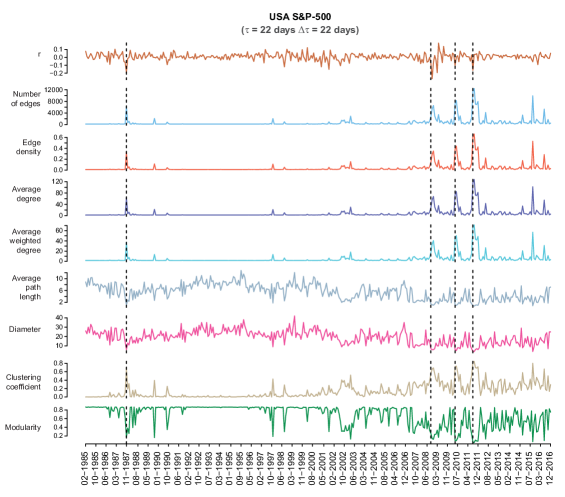
(a)
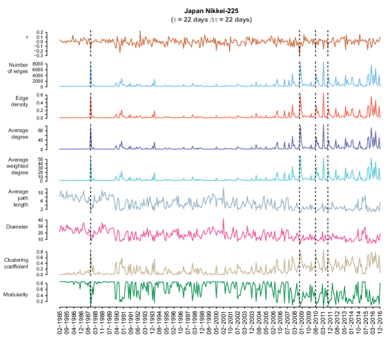
(b)

Figure S10: Evolution of network properties for (a) USA S&P-500 and (b) Japanese Nikkei-225 markets evaluated from the correlation matrices $\boldsymbol{C}_{\tau}(t)$ of window size $\tau=22$ days and a non-overlapping shift of $\Delta\tau=22$ days over the period (1985-2016). From top to bottom, we compare the plot of index log-returns $r$ with common network measures, namely, number of edges, edge density, average degree, average weighted degree, average path length, diameter, clustering coefficient and modularity.

Table S1: List of all stocks in USA S&P-500 market considered in this analysis. The first column gives the serial number, the second column gives the symbols, the third column gives the full name of the stock, the fourth column specifies the sector, and the fifth column has the abbreviation of the sector for the S&P-500 market.

S.No.	Code	Company Name	Sector	Abbreviation
1	CMCSA	Comcast Corp.	Consumer Discretionary	CD
2	DIS	The Walt Disney Company	Consumer Discretionary	CD
3	F	Ford Motor	Consumer Discretionary	CD
4	GPC	Genuine Parts	Consumer Discretionary	CD
5	GPS	Gap Inc.	Consumer Discretionary	CD
6	GT	Goodyear Tire & Rubber	Consumer Discretionary	CD
7	HAS	Hasbro Inc.	Consumer Discretionary	CD
8	HD	Home Depot	Consumer Discretionary	CD
9	HRB	Block H&R	Consumer Discretionary	CD
10	IPG	Interpublic Group	Consumer Discretionary	CD
11	JCP	J. C. Penney Company, Inc.	Consumer Discretionary	CD
12	JWN	Nordstrom	Consumer Discretionary	CD
13	LEG	Leggett & Platt	Consumer Discretionary	CD
14	LEN	Lennar Corp.	Consumer Discretionary	CD
15	LOW	Lowe’s Cos.	Consumer Discretionary	CD
16	MAT	Mattel Inc.	Consumer Discretionary	CD
17	MCD	McDonald’s Corp.	Consumer Discretionary	CD
18	NKE	Nike	Consumer Discretionary	CD
19	SHW	Sherwin-Williams	Consumer Discretionary	CD
20	TGT	Target Corp.	Consumer Discretionary	CD
21	VFC	V.F. Corp.	Consumer Discretionary	CD
22	WHR	Whirlpool Corp.	Consumer Discretionary	CD
23	ADM	Archer-Daniels-Midland Co	Consumer Staples	CS
24	AVP	Avon Products, Inc.	Consumer Staples	CS
25	CAG	Conagra Brands	Consumer Staples	CS
26	CL	Colgate-Palmolive	Consumer Staples	CS
27	CPB	Campbell Soup	Consumer Staples	CS
28	CVS	CVS Health	Consumer Staples	CS
29	GIS	General Mills	Consumer Staples	CS
30	HRL	Hormel Foods Corp.	Consumer Staples	CS
31	HSY	The Hershey Company	Consumer Staples	CS
32	K	Kellogg Co.	Consumer Staples	CS
33	KMB	Kimberly-Clark	Consumer Staples	CS
34	KO	Coca-Cola Company (The)	Consumer Staples	CS
35	KR	Kroger Co.	Consumer Staples	CS
36	MKC	McCormick & Co.	Consumer Staples	CS
37	MO	Altria Group Inc	Consumer Staples	CS
38	SYY	Sysco Corp.	Consumer Staples	CS
39	TAP	Molson Coors Brewing Company	Consumer Staples	CS
40	TSN	Tyson Foods	Consumer Staples	CS
41	WMT	Wal-Mart Stores	Consumer Staples	CS
42	APA	Apache Corporation	Energy	EG
43	COP	ConocoPhillips	Energy	EG
44	CVX	Chevron Corp.	Energy	EG
45	ESV	Ensco plc	Energy	EG
46	HAL	Halliburton Co.	Energy	EG
47	HES	Hess Corporation	Energy	EG
48	HP	Helmerich & Payne	Energy	EG
49	MRO	Marathon Oil Corp.	Energy	EG
50	MUR	Murphy Oil Corporation	Energy	EG

51	NBL	Noble Energy Inc	Energy	EG
52	NBR	Nabors Industries Ltd.	Energy	EG
53	SLB	Schlumberger Ltd.	Energy	EG
54	TSO	Tesoro Corp	Energy	EG
55	VLO	Valero Energy	Energy	EG
56	WMB	Williams Cos.	Energy	EG
57	XOM	Exxon Mobil Corp.	Energy	EG
58	AFL	AFLAC Inc	Financials	FN
59	AIG	American International Group, Inc.	Financials	FN
60	AON	Aon plc	Financials	FN
61	AXP	American Express Co	Financials	FN
62	BAC	Bank of America Corp	Financials	FN
63	BBT	BB&T Corporation	Financials	FN
64	BEN	Franklin Resources	Financials	FN
65	BK	The Bank of New York Mellon Corp.	Financials	FN
66	C	Citigroup Inc.	Financials	FN
67	CB	Chubb Limited	Financials	FN
68	CINF	Cincinnati Financial	Financials	FN
69	CMA	Comerica Inc.	Financials	FN
70	EFX	Equifax Inc.	Financials	FN
71	FHN	First Horizon National Corporation	Financials	FN
72	HBAN	Huntington Bancshares	Financials	FN
73	HCN	Welltower Inc.	Financials	FN
74	HST	Host Hotels & Resorts, Inc.	Financials	FN
75	JPM	JPMorgan Chase & Co.	Financials	FN
76	L	Loews Corp.	Financials	FN
77	LM	Legg Mason, Inc.	Financials	FN
78	LNC	Lincoln National	Financials	FN
79	LUK	Leucadia National Corp.	Financials	FN
80	MMC	Marsh & McLennan	Financials	FN
81	MTB	M&T Bank Corp.	Financials	FN
82	PSA	Public Storage	Financials	FN
83	SLM	SLM Corporation	Financials	FN
84	TMK	Torchmark Corp.	Financials	FN
85	TRV	The Travelers Companies Inc.	Financials	FN
86	USB	U.S. Bancorp	Financials	FN
87	VNO	Vornado Realty Trust	Financials	FN
88	WFC	Wells Fargo	Financials	FN
89	WY	Weyerhaeuser Corp.	Financials	FN
90	ZION	Zions Bancorp	Financials	FN
91	ABT	Abbott Laboratories	Health Care	HC
92	AET	Aetna Inc	Health Care	HC
93	AMGN	Amgen Inc	Health Care	HC
94	BAX	Baxter International Inc.	Health Care	HC
95	BCR	Bard (C.R.) Inc.	Health Care	HC
96	BDX	Becton Dickinson	Health Care	HC
97	BMY	Bristol-Myers Squibb	Health Care	HC
98	CAH	Cardinal Health Inc.	Health Care	HC
99	CI	CIGNA Corp.	Health Care	HC
100	HUM	Humana Inc.	Health Care	HC

101	JNJ	Johnson & Johnson	Health Care	HC
102	LLY	Lilly (Eli) & Co.	Health Care	HC
103	MDT	Medtronic plc	Health Care	HC
104	MRK	Merck & Co.	Health Care	HC
105	MYL	Mylan N.V.	Health Care	HC
106	SYK	Stryker Corp.	Health Care	HC
107	THC	Tenet Healthcare Corp	Health Care	HC
108	TMO	Thermo Fisher Scientific	Health Care	HC
109	UNH	United Health Group Inc.	Health Care	HC
110	VAR	Varian Medical Systems	Health Care	HC
111	AVY	Avery Dennison Corp	Industrials	ID
112	BA	Boeing Company	Industrials	ID
113	CAT	Caterpillar Inc.	Industrials	ID
114	CMI	Cummins Inc.	Industrials	ID
115	CSX	CSX Corp.	Industrials	ID
116	CTAS	Cintas Corporation	Industrials	ID
117	DE	Deere & Co.	Industrials	ID
118	DHR	Danaher Corp.	Industrials	ID
119	DNB	The Dun & Bradstreet Corporation	Industrials	ID
120	DOV	Dover Corp.	Industrials	ID
121	EMR	Emerson Electric Company	Industrials	ID
122	ETN	Eaton Corporation	Industrials	ID
123	EXPD	Expeditors International	Industrials	ID
124	FDX	FedEx Corporation	Industrials	ID
125	FLS	Flowserve Corporation	Industrials	ID
126	GD	General Dynamics	Industrials	ID
127	GE	General Electric	Industrials	ID
128	GLW	Corning Inc.	Industrials	ID
129	GWW	Grainger (W.W.) Inc.	Industrials	ID
130	HON	Honeywell Int’l Inc.	Industrials	ID
131	IR	Ingersoll-Rand PLC	Industrials	ID
132	ITW	Illinois Tool Works	Industrials	ID
133	JEC	Jacobs Engineering Group	Industrials	ID
134	LMT	Lockheed Martin Corp.	Industrials	ID
135	LUV	Southwest Airlines	Industrials	ID
136	MAS	Masco Corp.	Industrials	ID
137	MMM	3M Company	Industrials	ID
138	ROK	Rockwell Automation Inc.	Industrials	ID
139	RTN	Raytheon Co.	Industrials	ID
140	TXT	Textron Inc.	Industrials	ID
141	UNP	Union Pacific	Industrials	ID
142	UTX	United Technologies	Industrials	ID
143	AAPL	Apple Inc.	Information Technology	IT
144	ADI	Analog Devices, Inc.	Information Technology	IT
145	ADP	Automatic Data Processing	Information Technology	IT
146	AMAT	Applied Materials Inc	Information Technology	IT
147	AMD	Advanced Micro Devices Inc	Information Technology	IT
148	CA	CA, Inc.	Information Technology	IT
149	HPQ	HP Inc.	Information Technology	IT
150	HRS	Harris Corporation	Information Technology	IT

151	IBM	International Business Machines	Information Technology	IT
152	INTC	Intel Corp.	Information Technology	IT
153	KLAC	KLA-Tencor Corp.	Information Technology	IT
154	LRCX	Lam Research	Information Technology	IT
155	MSI	Motorola Solutions Inc.	Information Technology	IT
156	MU	Micron Technology	Information Technology	IT
157	TSS	Total System Services, Inc.	Information Technology	IT
158	TXN	Texas Instruments	Information Technology	IT
159	WDC	Western Digital	Information Technology	IT
160	XRX	Xerox Corp.	Information Technology	IT
161	AA	Alcoa Corporation	Materials	MT
162	APD	Air Products & Chemicals Inc	Materials	MT
163	BLL	Ball Corp	Materials	MT
164	BMS	Bemis Company, Inc.	Materials	MT
165	CLF	Cleveland-Cliffs Inc.	Materials	MT
166	DD	DuPont	Materials	MT
167	ECL	Ecolab Inc.	Materials	MT
168	FMC	FMC Corporation	Materials	MT
169	IFF	Intl Flavors & Fragrances	Materials	MT
170	IP	International Paper	Materials	MT
171	NEM	Newmont Mining Corporation	Materials	MT
172	PPG	PPG Industries	Materials	MT
173	VMC	Vulcan Materials	Materials	MT
174	CTL	CenturyLink Inc	Telecommunication Services	TC
175	FTR	Frontier Communications Corporation	Telecommunication Services	TC
176	S	Sprint Nextel Corp.	Telecommunication Services	TC
177	T	AT&T Inc	Telecommunication Services	TC
178	VZ	Verizon Communications	Telecommunication Services	TC
179	AEP	American Electric Power	Utilities	UT
180	CMS	CMS Energy	Utilities	UT
181	CNP	CenterPoint Energy	Utilities	UT
182	D	Dominion Energy	Utilities	UT
183	DTE	DTE Energy Co.	Utilities	UT
184	ED	Consolidated Edison	Utilities	UT
185	EIX	Edison Int’l	Utilities	UT
186	EQT	EQT Corporation	Utilities	UT
187	ETR	Entergy Corp.	Utilities	UT
188	EXC	Exelon Corp.	Utilities	UT
189	NEE	NextEra Energy	Utilities	UT
190	NI	NiSource Inc.	Utilities	UT
191	PNW	Pinnacle West Capital	Utilities	UT
192	SO	Southern Co.	Utilities	UT
193	WEC	Wec Energy Group Inc	Utilities	UT
194	XEL	Xcel Energy Inc	Utilities	UT

Table S2: List of all stocks in Japan Nikkei-225 market considered in this analysis. The first column gives the serial number, the second column gives the symbols, the third column gives the full name of the stock, the fourth column specifies the sector, and the fifth column has the abbreviation of the sector for the Nikkei-225 market.

S.No.	Code	Company Name	Sector	Abbreviation
1	S-8801	MITSUI FUDOSAN CO., LTD.	Capital Goods	CG
2	S-8802	MITSUBISHI ESTATE CO., LTD.	Capital Goods	CG
3	S-8804	TOKYO TATEMONO CO., LTD.	Capital Goods	CG
4	S-8830	SUMITOMO REALTY & DEVELOPMENT CO., LTD.	Capital Goods	CG
5	S-7003	MITSUI ENG. & SHIPBUILD. CO., LTD.	Capital Goods	CG
6	S-7012	KAWASAKI HEAVY IND., LTD.	Capital Goods	CG
7	S-9202	ANA HOLDINGS INC.	Capital Goods	CG
8	S-1801	TAISEI CORP.	Capital Goods	CG
9	S-1802	OBAYASHI CORP.	Capital Goods	CG
10	S-1803	SHIMIZU CORP.	Capital Goods	CG
11	S-1808	HASEKO CORP.	Capital Goods	CG
12	S-1812	KAJIMA CORP.	Capital Goods	CG
13	S-1925	DAIWA HOUSE IND. CO., LTD.	Capital Goods	CG
14	S-1928	SEKISUI HOUSE, LTD.	Capital Goods	CG
15	S-1963	JGC CORP.	Capital Goods	CG
16	S-5631	THE JAPAN STEEL WORKS, LTD.	Capital Goods	CG
17	S-6103	OKUMA CORP.	Capital Goods	CG
18	S-6113	AMADA HOLDINGS CO., LTD.	Capital Goods	CG
19	S-6301	KOMATSU LTD.	Capital Goods	CG
20	S-6302	SUMITOMO HEAVY IND., LTD.	Capital Goods	CG
21	S-6305	HITACHI CONST. MACH. CO., LTD.	Capital Goods	CG
22	S-6326	KUBOTA CORP.	Capital Goods	CG
23	S-6361	EBARA CORP.	Capital Goods	CG
24	S-6366	CHIYODA CORP.	Capital Goods	CG
25	S-6367	DAIKIN INDUSTRIES, LTD.	Capital Goods	CG
26	S-6471	NSK LTD.	Capital Goods	CG
27	S-6472	NTN CORP.	Capital Goods	CG
28	S-6473	JTEKT CORP.	Capital Goods	CG
29	S-7004	HITACHI ZOSEN CORP.	Capital Goods	CG
30	S-7011	MITSUBISHI HEAVY IND., LTD.	Capital Goods	CG
31	S-7013	IHI CORP.	Capital Goods	CG
32	S-7911	TOPPAN PRINTING CO., LTD.	Capital Goods	CG
33	S-7912	DAI NIPPON PRINTING CO., LTD.	Capital Goods	CG
34	S-7951	YAMAHA CORP.	Capital Goods	CG
35	S-1332	NIPPON SUISAN KAISHA, LTD.	Consumer Goods	CN
36	S-2002	NISSHIN SEIFUN GROUP INC.	Consumer Goods	CN
37	S-2282	NH FOODS LTD.	Consumer Goods	CN
38	S-2501	SAPPORO HOLDINGS LTD.	Consumer Goods	CN
39	S-2502	ASAHI GROUP HOLDINGS, LTD.	Consumer Goods	CN
40	S-2503	KIRIN HOLDINGS CO., LTD.	Consumer Goods	CN
41	S-2531	TAKARA HOLDINGS INC.	Consumer Goods	CN
42	S-2801	KIKKOMAN CORP.	Consumer Goods	CN
43	S-2802	AJINOMOTO CO., INC.	Consumer Goods	CN
44	S-2871	NICHIREI CORP.	Consumer Goods	CN
45	S-8233	TAKASHIMAYA CO., LTD.	Consumer Goods	CN
46	S-8252	MARUI GROUP CO., LTD.	Consumer Goods	CN
47	S-8267	AEON CO., LTD.	Consumer Goods	CN
48	S-9602	TOHO CO., LTD	Consumer Goods	CN
49	S-9681	TOKYO DOME CORP.	Consumer Goods	CN
50	S-9735	SECOM CO., LTD.	Consumer Goods	CN

51	S-8331	THE CHIBA BANK, LTD.	Financials	FN
52	S-8355	THE SHIZUOKA BANK, LTD.	Financials	FN
53	S-8253	CREDIT SAISON CO., LTD.	Financials	FN
54	S-8601	DAIWA SECURITIES GROUP INC.	Financials	FN
55	S-8604	NOMURA HOLDINGS, INC.	Financials	FN
56	S-3405	KURARAY CO., LTD.	Materials	MT
57	S-3407	ASAHI KASEI CORP.	Materials	MT
58	S-4004	SHOWA DENKO K.K.	Materials	MT
59	S-4005	SUMITOMO CHEMICAL CO., LTD.	Materials	MT
60	S-4021	NISSAN CHEMICAL IND., LTD.	Materials	MT
61	S-4042	TOSOH CORP.	Materials	MT
62	S-4043	TOKUYAMA CORP.	Materials	MT
63	S-4061	DENKA CO., LTD.	Materials	MT
64	S-4063	SHIN-ETSU CHEMICAL CO., LTD.	Materials	MT
65	S-4183	MITSUI CHEMICALS, INC.	Materials	MT
66	S-4208	UBE INDUSTRIES, LTD.	Materials	MT
67	S-4272	NIPPON KAYAKU CO., LTD.	Materials	MT
68	S-4452	KAO CORP.	Materials	MT
69	S-4901	FUJIFILM HOLDINGS CORP.	Materials	MT
70	S-4911	SHISEIDO CO., LTD.	Materials	MT
71	S-6988	NITTO DENKO CORP.	Materials	MT
72	S-5002	SHOWA SHELL SEKIYU K.K.	Materials	MT
73	S-5201	ASAHI GLASS CO., LTD.	Materials	MT
74	S-5202	NIPPON SHEET GLASS CO., LTD.	Materials	MT
75	S-5214	NIPPON ELECTRIC GLASS CO., LTD.	Materials	MT
76	S-5232	SUMITOMO OSAKA CEMENT CO., LTD.	Materials	MT
77	S-5233	TAIHEIYO CEMENT CORP.	Materials	MT
78	S-5301	TOKAI CARBON CO., LTD.	Materials	MT
79	S-5332	TOTO LTD.	Materials	MT
80	S-5333	NGK INSULATORS, LTD.	Materials	MT
81	S-5706	MITSUI MINING & SMELTING CO.	Materials	MT
82	S-5707	TOHO ZINC CO., LTD.	Materials	MT
83	S-5711	MITSUBISHI MATERIALS CORP.	Materials	MT
84	S-5713	SUMITOMO METAL MINING CO., LTD.	Materials	MT
85	S-5714	DOWA HOLDINGS CO., LTD.	Materials	MT
86	S-5715	FURUKAWA CO., LTD.	Materials	MT
87	S-5801	FURUKAWA ELECTRIC CO., LTD.	Materials	MT
88	S-5802	SUMITOMO ELECTRIC IND., LTD.	Materials	MT
89	S-5803	FUJIKURA LTD.	Materials	MT
90	S-5901	TOYO SEIKAN GROUP HOLDINGS, LTD.	Materials	MT
91	S-3865	HOKUETSU KISHU PAPER CO., LTD.	Materials	MT
92	S-3861	OJI HOLDINGS CORP.	Materials	MT
93	S-5101	THE YOKOHAMA RUBBER CO., LTD.	Materials	MT
94	S-5108	BRIDGESTONE CORP.	Materials	MT
95	S-5401	NIPPON STEEL & SUMITOMO METAL CORP.	Materials	MT
96	S-5406	KOBE STEEL, LTD.	Materials	MT
97	S-5541	PACIFIC METALS CO., LTD.	Materials	MT
98	S-3101	TOYOBO CO., LTD.	Materials	MT
99	S-3103	UNITIKA, LTD.	Materials	MT
100	S-3401	TEIJIN LTD.	Materials	MT

101	S-3402	TORAY INDUSTRIES, INC.	Materials	MT
102	S-8001	ITOCHU CORP.	Materials	MT
103	S-8002	MARUBENI CORP.	Materials	MT
104	S-8015	TOYOTA TSUSHO CORP.	Materials	MT
105	S-8031	MITSUI & CO., LTD.	Materials	MT
106	S-8053	SUMITOMO CORP.	Materials	MT
107	S-8058	MITSUBISHI CORP.	Materials	MT
108	S-4151	KYOWA HAKKO KIRIN CO., LTD.	Pharmaceuticals	PH
109	S-4503	ASTELLAS PHARMA INC.	Pharmaceuticals	PH
110	S-4506	SUMITOMO DAINIPPON PHARMA CO., LTD.	Pharmaceuticals	PH
111	S-4507	SHIONOGI & CO., LTD.	Pharmaceuticals	PH
112	S-4519	CHUGAI PHARMACEUTICAL CO., LTD.	Pharmaceuticals	PH
113	S-4523	EISAI CO., LTD.	Pharmaceuticals	PH
114	S-7201	NISSAN MOTOR CO., LTD.	Information Technology	IT
115	S-7202	ISUZU MOTORS LTD.	Information Technology	IT
116	S-7205	HINO MOTORS, LTD.	Information Technology	IT
117	S-7261	MAZDA MOTOR CORP.	Information Technology	IT
118	S-7267	HONDA MOTOR CO., LTD.	Information Technology	IT
119	S-7270	SUBARU CORP.	Information Technology	IT
120	S-7272	YAMAHA MOTOR CO., LTD.	Information Technology	IT
121	S-3105	NISSHINBO HOLDINGS INC.	Information Technology	IT
122	S-6479	MINEBEA MITSUMI INC.	Information Technology	IT
123	S-6501	HITACHI, LTD.	Information Technology	IT
124	S-6502	TOSHIBA CORP.	Information Technology	IT
125	S-6503	MITSUBISHI ELECTRIC CORP.	Information Technology	IT
126	S-6504	FUJI ELECTRIC CO., LTD.	Information Technology	IT
127	S-6506	YASKAWA ELECTRIC CORP.	Information Technology	IT
128	S-6508	MEIDENSHA CORP.	Information Technology	IT
129	S-6701	NEC CORP.	Information Technology	IT
130	S-6702	FUJITSU LTD.	Information Technology	IT
131	S-6703	OKI ELECTRIC IND. CO., LTD.	Information Technology	IT
132	S-6752	PANASONIC CORP.	Information Technology	IT
133	S-6758	SONY CORP.	Information Technology	IT
134	S-6762	TDK CORP.	Information Technology	IT
135	S-6770	ALPS ELECTRIC CO., LTD.	Information Technology	IT
136	S-6773	PIONEER CORP.	Information Technology	IT
137	S-6841	YOKOGAWA ELECTRIC CORP.	Information Technology	IT
138	S-6902	DENSO CORP.	Information Technology	IT
139	S-6952	CASIO COMPUTER CO., LTD.	Information Technology	IT
140	S-6954	FANUC CORP.	Information Technology	IT
141	S-6971	KYOCERA CORP.	Information Technology	IT
142	S-6976	TAIYO YUDEN CO., LTD.	Information Technology	IT
143	S-7752	RICOH CO., LTD.	Information Technology	IT
144	S-8035	TOKYO ELECTRON LTD.	Information Technology	IT
145	S-4543	TERUMO CORP.	Information Technology	IT
146	S-4902	KONICA MINOLTA, INC.	Information Technology	IT
147	S-7731	NIKON CORP.	Information Technology	IT
148	S-7733	OLYMPUS CORP.	Information Technology	IT
149	S-7762	CITIZEN WATCH CO., LTD.	Information Technology	IT
150	S-9501	TOKYO ELECTRIC POWER COMPANY HOLDINGS, I	Transportation & Utilities	TU

151	S-9502	CHUBU ELECTRIC POWER CO., INC.	Transportation & Utilities	TU
152	S-9503	THE KANSAI ELECTRIC POWER CO., INC.	Transportation & Utilities	TU
153	S-9531	TOKYO GAS CO., LTD.	Transportation & Utilities	TU
154	S-9532	OSAKA GAS CO., LTD.	Transportation & Utilities	TU
155	S-9062	NIPPON EXPRESS CO., LTD.	Transportation & Utilities	TU
156	S-9064	YAMATO HOLDINGS CO., LTD.	Transportation & Utilities	TU
157	S-9101	NIPPON YUSEN K.K.	Transportation & Utilities	TU
158	S-9104	MITSUI O.S.K.LINES, LTD.	Transportation & Utilities	TU
159	S-9107	KAWASAKI KISEN KAISHA, LTD.	Transportation & Utilities	TU
160	S-9001	TOBU RAILWAY CO., LTD.	Transportation & Utilities	TU
161	S-9005	TOKYU CORP.	Transportation & Utilities	TU
162	S-9007	ODAKYU ELECTRIC RAILWAY CO., LTD.	Transportation & Utilities	TU
163	S-9008	KEIO CORP.	Transportation & Utilities	TU
164	S-9009	KEISEI ELECTRIC RAILWAY CO., LTD.	Transportation & Utilities	TU
165	S-9301	MITSUBISHI LOGISTICS CORP.	Transportation & Utilities	TU

Table S3: Number of edges ($\#$ Edges) and communities ($\#$ Communities) in threshold networks $S_{\tau}(t)$ for USA S&P-500 market at eight distinct epochs of $\tau=22$ days ending on trading days 23-01-2006, 10-05-2006, 29-06-2006, 06-11-2006, 07-01-2011, 04-05-2011, 02-09-2011, and 03-02-2012 (around the US Housing bubble period (2006-2007) and August 2011 stock markets fall crisis), constructed using four different thresholds, $C_{ij}(t)\geq 0.55$, $C_{ij}(t)\geq 0.65$, $C_{ij}(t)\geq 0.75$, and $C_{ij}(t)\geq 0.85$.

	US Housing Bubble Networks				August 2011 Fall Crash Networks
End Date	23-01-2006				07-01-2011
Threshold	0.55	0.65	0.75	0.85	0.55	0.65	0.75	0.85
# Edges	1949	733	251	193	645	284	197	193
# Communities	5	13	13	14	9	11	14	14
End date	10-05-2006				04-05-2011
Threshold	0.55	0.65	0.75	0.85	0.55	0.65	0.75	0.85
# Edges	838	351	220	193	1378	542	245	194
# Communities	7	12	16	15	6	11	16	16
End date	29-06-2006				02-09-2011
Threshold	0.55	0.65	0.75	0.85	0.55	0.65	0.75	0.85
# Edges	6291	3138	996	250	18258	17697	16004	9906
# Communities	3	5	11	15	3	3	4	3
End date	06-11-2006				03-02-2012
Threshold	0.55	0.65	0.75	0.85	0.55	0.65	0.75	0.85
# Edges	677	287	220	193	931	328	198	193
# Communities	9	12	14	14	8	12	15	16

References

- Anderson (1972) P. W. Anderson, Science 177, 393 (1972).
- Vemuri (1978) V. Vemuri, Modeling of Complex Systems: An Introduction (Academic Press, New York, 1978).
- Gell-Mann (1995) M. Gell-Mann, Complexity 1, 16 (1995).
- Mantegna and Stanley (2007) R. N. Mantegna and H. E. Stanley, An introduction to econophysics: correlations and complexity in finance (Cambridge University Press, Cambridge, 2007).
- Bouchaud and Potters (2003) J.-P. Bouchaud and M. Potters, Theory of Financial Risk and Derivative Pricing: from Statistical Physics to Risk Management (Cambridge University Press, 2003).
- Sinha et al. (2010) S. Sinha, A. Chatterjee, A. Chakraborti, and B. K. Chakrabarti, Econophysics: an introduction (John Wiley & Sons, 2010).
- Chakraborti et al. (2011) A. Chakraborti, I. Muni Toke, M. Patriarca, and F. Abergel, Quantitative Finance 11, 991 (2011).
- Chakraborti et al. (2015) A. Chakraborti, D. Challet, A. Chatterjee, M. Marsili, Y.-C. Zhang, and B. K. Chakrabarti, Physics Reports 552, 1 (2015).
- Battiston et al. (2016) S. Battiston, J. D. Farmer, A. Flache, D. Garlaschelli, A. G. Haldane, H. Heesterbeek, C. Hommes, C. Jaeger, R. May, and M. Scheffer, Science 351, 818 (2016).
- Lux and Westerhoff (2009) T. Lux and F. Westerhoff, Nature Physics 5, 2 (2009).
- Mantegna (1999a) R. N. Mantegna, Computer Physics Communications 121-122, 153 (1999a).
- Mantegna (1999b) R. N. Mantegna, The European Physical Journal B 11, 193 (1999b).
- Laloux et al. (1999) L. Laloux, P. Cizeau, J.-P. Bouchaud, and M. Potters, Physical Review Letters 83, 1467 (1999).
- Plerou et al. (1999) V. Plerou, P. Gopikrishnan, B. Rosenow, L. A. Nunes Amaral, and H. E. Stanley, Physical Review Letters 83, 1471 (1999).
- Gopikrishnan et al. (2001) P. Gopikrishnan, B. Rosenow, V. Plerou, and H. E. Stanley, Physical Review E 64, 035106 (2001).
- Kullmann et al. (2002) L. Kullmann, J. Kertész, and K. Kaski, Physical Review E 66, 026125 (2002).
- Plerou et al. (2002) V. Plerou, P. Gopikrishnan, B. Rosenow, L. A. N. Amaral, T. Guhr, and H. E. Stanley, Physical Review E 65, 066126 (2002).
- Onnela et al. (2003) J.-P. Onnela, A. Chakraborti, K. Kaski, J. Kertesz, and A. Kanto, Physical Review E 68, 056110 (2003).
- Tumminello et al. (2005) M. Tumminello, T. Aste, T. Di Matteo, and R. N. Mantegna, Proceedings of the National Academy of Sciences 102, 10421 (2005).
- Pharasi et al. (2018) H. K. Pharasi, K. Sharma, R. Chatterjee, A. Chakraborti, F. Leyvraz, and T. H. Seligman, New Journal of Physics 20, 103041 (2018).
- Pharasi et al. (2019) H. K. Pharasi, K. Sharma, A. Chakraborti, and T. H. Seligman, “Complex market dynamics in the light of random matrix theory,” in New Perspectives and Challenges in Econophysics and Sociophysics, edited by F. Abergel, B. K. Chakrabarti, A. Chakraborti, N. Deo, and K. Sharma (Springer International Publishing, Cham, 2019) pp. 13–34.
- Chakraborti et al. (2020a) A. Chakraborti, K. Sharma, H. K. Pharasi, K. Shuvo Bakar, S. Das, and T. H. Seligman, New Journal of Physics 22, 063043 (2020a).
- Chi et al. (2010) K. T. Chi, J. Liu, and F. C. Lau, Journal of Empirical Finance 17, 659 (2010).
- Tumminello et al. (2007) M. Tumminello, T. Di Matteo, T. Aste, and R. N. Mantegna, The European Physical Journal B 55, 209 (2007).
- Tumminello et al. (2010) M. Tumminello, F. Lillo, and R. N. Mantegna, Journal of economic behavior & organization 75, 40 (2010).
- Miccichè et al. (2003) S. Miccichè, G. Bonanno, F. Lillo, and R. N. Mantegna, Physica A: Statistical Mechanics and its Applications 324, 66 (2003).
- Kumar and Deo (2012) S. Kumar and N. Deo, Physical Review E 86, 026101 (2012).
- Almog and Shmueli (2019) A. Almog and E. Shmueli, Scientific Reports 9, 10832 (2019).
- Wang et al. (2019) J. Wang, C. Lin, and Y. Wang, Complexity 2019, 1817248 (2019).
- Chakraborti et al. (2020b) A. Chakraborti, Hrishidev, K. Sharma, and H. K. Pharasi, Journal of Physics: Complexity 2, 015002 (2020b).
- Kukreti et al. (2020) V. Kukreti, H. K. Pharasi, P. Gupta, and S. Kumar, Frontiers in Physics 8, 323 (2020).
- Nie and Song (2018) C.-x. Nie and F.-t. Song, Entropy 20, 177 (2018).
- Stepanov et al. (2015) Y. Stepanov, P. Rinn, T. Guhr, J. Peinke, and R. Schäfer, Journal of Statistical Mechanics: Theory and Experiment 2015, P08011 (2015).
- Rinn et al. (2015) P. Rinn, Y. Stepanov, J. Peinke, T. Guhr, and R. Schäfer, EPL 110, 68003 (2015).
- Chetalova et al. (2015) D. Chetalova, R. Schäfer, and T. Guhr, Journal of Statistical Mechanics: Theory and Experiment 2015, P01029 (2015).
- Heckens et al. (2020) A. J. Heckens, S. M. Krause, and T. Guhr, Journal of Statistical Mechanics: Theory and Experiment 2020, P103402 (2020).
- Wang et al. (2020) S. Wang, S. Gartzke, M. Schreckenberg, and T. Guhr, Journal of Statistical Mechanics: Theory and Experiment 2020, P103404 (2020).
- Jost (2017) J. Jost, Riemannian Geometry and Geometric Analysis, 7th ed. (Springer International Publishing, 2017).
- Carlsson (2009) G. Carlsson, Bulletin of the American Mathematical Society 46, 255 (2009).
- Krioukov et al. (2010) D. Krioukov, F. Papadopoulos, M. Kitsak, A. Vahdat, and M. Boguná, Physical Review E 82, 036106 (2010).
- Bianconi (2015) G. Bianconi, EPL 111, 56001 (2015).
- Sandhu et al. (2015) R. Sandhu, T. Georgiou, E. Reznik, L. Zhu, I. Kolesov, Y. Senbabaoglu, and A. Tannenbaum, Scientific Reports 5, 12323 (2015).
- Sreejith et al. (2016) R. P. Sreejith, K. Mohanraj, J. Jost, E. Saucan, and A. Samal, Journal of Statistical Mechanics: Theory and Experiment 2016, P063206 (2016).
- Bianconi and Rahmede (2017) G. Bianconi and C. Rahmede, Scientific Reports 7, 41974 (2017).
- Kartun-Giles and Bianconi (2019) A. P. Kartun-Giles and G. Bianconi, Chaos, Solitons & Fractals: X 1, 100004 (2019).
- Iacopini et al. (2019) I. Iacopini, G. Petri, A. Barrat, and V. Latora, Nature communications 10, 2485 (2019).
- Kannan et al. (2019) H. Kannan, E. Saucan, I. Roy, and A. Samal, Scientific reports 9, 13817 (2019).
- Samal et al. (2018) A. Samal, R. P. Sreejith, J. Gu, S. Liu, E. Saucan, and J. Jost, Scientific Reports 8, 8650 (2018).
- Ni et al. (2015) C. Ni, Y. Lin, J. Gao, X. D. Gu, and E. Saucan, in 2015 IEEE Conference on Computer Communications (INFOCOM) (IEEE, 2015) pp. 2758–2766.
- Sandhu et al. (2016) R. S. Sandhu, T. T. Georgiou, and A. R. Tannenbaum, Science Advances 2, e1501495 (2016).
- Ni et al. (2019) C. Ni, Y. Lin, F. Luo, and J. Gao, Scientific Reports 9, 9984 (2019).
- Ollivier (2007) Y. Ollivier, Comptes Rendus Mathematique 345, 643 (2007).
- Ollivier (2009) Y. Ollivier, Journal of Functional Analysis 256, 810 (2009).
- Aste et al. (2005) T. Aste, T. Di Matteo, and S. Hyde, Physica A: Statistical Mechanics and its Applications 346, 20 (2005).
- Saucan et al. (2020) E. Saucan, A. Samal, and J. Jost, Network Science , 1 (2020).
- Saucan (2012) E. Saucan, Journal of Mathematical Imaging and Vision 43, 143 (2012).
- Scheffer et al. (2012) M. Scheffer, S. R. Carpenter, T. M. Lenton, J. Bascompte, W. Brock, V. Dakos, J. van de Koppel, I. A. van de Leemput, S. A. Levin, E. H. van Nes, M. Pascual, and J. Vandermeer, Science 338, 344 (2012).
- Lin and Yau (2010) Y. Lin and S.-T. Yau, Math. Res. Lett. 17, 343 (2010).
- Lin et al. (2011) Y. Lin, L. Lu, and S.-T. Yau, Tohoku Mathematical Journal 63, 605 (2011).
- Bauer et al. (2012) F. Bauer, J. Jost, and S. Liu, Math. Res. Lett. 19, 1185 (2012).
- Jost and Liu (2014) J. Jost and S. Liu, Discrete & Computational Geometry 51, 300 (2014).
- Sia et al. (2019) J. Sia, E. Jonckheere, and P. Bogdan, Scientific Reports 9, 9800 (2019).
- Vaserstein (1969) L. N. Vaserstein, Probl. Peredachi Inf. 5, 64 (1969).
- Forman (2003) R. Forman, Discrete & Computational Geometry 29, 323 (2003).
- Saucan et al. (2019a) E. Saucan, R. P. Sreejith, R. P. Vivek-Ananth, J. Jost, and A. Samal, Chaos, Solitons & Fractals 118, 347 (2019a).
- Sreejith et al. (2017) R. P. Sreejith, J. Jost, E. Saucan, and A. Samal, Chaos, Solitons & Fractals 101, 50 (2017).
- Menger (1930) K. Menger, Mathematische Annalen 103, 466 (1930).
- Saucan et al. (2019b) E. Saucan, A. Samal, and J. Jost, in International Conference on Complex Networks and their Applications (Springer, 2019) pp. 943–954.
- Haantjes (1947) J. Haantjes, Proc. Kon. Ned. Akad. v. Wetenseh., Amsterdam 50, 302 (1947).
- (70) “Yahoo finance database,” https://finance.yahoo.co.jp/, accessed on 7th July, 2017.
- Prim (1957) R. C. Prim, The Bell System Technical Journal 36, 1389 (1957).
- Latora and Marchiori (2001) V. Latora and M. Marchiori, Physical Review Letters 87, 198701 (2001).
- Girvan and Newman (2002) M. Girvan and M. E. J. Newman, Proceedings of the National Academy of Sciences USA 99, 7821 (2002).
- Blondel et al. (2008) V. D. Blondel, J.-L. Guillaume, R. Lambiotte, and E. Lefebvre, Journal of Statistical Mechanics: Theory and Experiment 2008, P10008 (2008).
- Solé and Valverde (2004) R. V. Solé and S. Valverde, in Complex Networks (Springer, 2004) pp. 189–207.
- Hagberg et al. (2008) A. Hagberg, P. Swart, and D. S. Chult, Exploring network structure, dynamics, and function using NetworkX, Tech. Rep. (Los Alamos National Laboratory (LANL), Los Alamos, NM (United States), 2008).
- Bollerslev (1986) T. Bollerslev, Journal of Econometrics 31, 307 (1986).
- Cra (a) “List of stock market crashes and bear markets,” https://en.wikipedia.org/wiki/List_of_stock_market_crashes_and_bear_markets (a), accessed on 7th July, 2019.
- (79) “Bull markets,” https://bullmarkets.co/u-s-stock-market-in-1996/, accessed on 7th July, 2019.
- (80) “United states housing bubble,” https://en.wikipedia.org/wiki/United_States_housing_bubble, accessed on 7th July, 2019.
- Cra (b) “A short history of stock market crashes,” https://www.cnbc.com/2016/08/24/a-short-history-of-stock-market-crashes.html (b), accessed on 7th July, 2019.
- (82) “Stock market selloff,” https://en.wikipedia.org/wiki/2015-16_stock_market_selloff, accessed on 7th July, 2019.
- (83) “August 2011 stock markets fall,” https://en.wikipedia.org/wiki/August_2011_stock_markets_fall, accessed on 13th August, 2020.
- Kenett et al. (2010) D. Y. Kenett, M. Tumminello, A. Madi, G. Gur-Gershgoren, R. N. Mantegna, and E. Ben-Jacob, PloS One 5, e15032 (2010).
- San Miguel et al. (2012) M. San Miguel, J. H. Johnson, J. Kertesz, K. Kaski, A. Díaz-Guilera, R. S. MacKay, V. Loreto, P. Érdi, and D. Helbing, The European Physical Journal Special Topics 214, 245 (2012).
- Millington and Niranjan (2020) T. Millington and M. Niranjan, Applied Network Science 5, 1 (2020).
- Sharma et al. (2017) K. Sharma, S. Shah, A. S. Chakrabarti, and A. Chakraborti, in Economic Foundations for Social Complexity Science (Springer, 2017) pp. 211–238.