Are scene graphs good enough to improve Image Captioning?

Abstract

Many top-performing image captioning models rely solely on object features computed with an object detection model to generate image descriptions. However, recent studies propose to directly use scene graphs to introduce information about object relations into captioning, hoping to better describe interactions between objects. In this work, we thoroughly investigate the use of scene graphs in image captioning. We empirically study whether using additional scene graph encoders can lead to better image descriptions and propose a conditional graph attention network (C-GAT), where the image captioning decoder state is used to condition the graph updates. Finally, we determine to what extent noise in the predicted scene graphs influence caption quality. Overall, we find no significant difference between models that use scene graph features and models that only use object detection features across different captioning metrics, which suggests that existing scene graph generation models are still too noisy to be useful in image captioning. Moreover, although the quality of predicted scene graphs is very low in general, when using high quality scene graphs we obtain gains of up to 3.3 CIDEr compared to a strong Bottom-Up Top-Down baseline.

1 Introduction

Scene understanding is a complex and intricate activity which humans perform effortlessly but that computational models still struggle with. An important backbone of scene understanding is being able to detect objects and relations between objects in an image, and scene graphs (Johnson et al., 2015; Anderson et al., 2016) are a closely related data structure that explicitly annotates an image with its objects and relations in context. Scene graphs can be used to improve important visual tasks that require scene understanding, e.g. image indexing and search (Johnson et al., 2015) or scene construction and generation (Johnson et al., 2017, 2018), and there is evidence that they can also be used to improve image captioning (Yang et al., 2019; Li and Jiang, 2019). However, the de facto standard in top-performing image captioning models to date use strong object features only, e.g. obtained with a pretrained Faster R-CNN (Ren et al., 2015), and no explicit relation information (Anderson et al., 2018; Lu et al., 2018; Yu et al., 2019a).

One possible explanation to this observation is that by using detected objects we already capture the more important information that characterises a scene, and that relation information is already implicitly learned in such models. Another explanation is that relations are simply not as important as we hypothesise and that we gain no valuable extra information by adding them. In this work, we investigate these empirical observations in more detail and strive to answer the following research questions: (i) Can we improve image captioning by explicitly supervising a model with information about object relations? (ii) How does the content of the captions improve when utilising scene graphs? (iii) How does scene graph quality impact the quality of the captions?

The most recent best-performing image captioning models make use of the Transformer architecture (Vaswani et al., 2017; Li et al., 2019; Yu et al., 2019b). However, in this paper we build upon the influential Bottom-Up Top-Down architecture (Anderson et al., 2018) which uses LSTMs, and since we want to measure to what extent scene graphs are helpful or not, we remove any “extras” to make model comparison easier, e.g. reinforcement learning step after cross-entropy training, ensembling at inference time, etc.

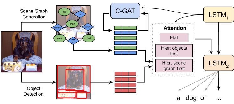
Figure 1: We use object features from an object detection model and scene graph features from a scene graph generation model in image captioning. We use conditional graph attention (C-GAT)to encode scene graph features, and flat vs. hierarchical attention mechanisms are used to incorporate both feature sets into an LSTM decoder.

Scene graph generation (SGG) is the task where given an image a model predicts a graph with its objects and their relations. We use a pretrained SGG model (Xu et al., 2017) to obtain and inject explicit relation information into image captioning, and investigate different image captioning model architectures that incorporate object and relation features, similarly to Li and Jiang (2019); Wang et al. (2019). We propose an extension to graph attention networks (Veličković et al., 2018) which we call conditional graph attention (C-GAT), where we condition the updates of the scene graph features on the current image captioning decoder state. Finally, we conduct an in-depth analysis of the captions produced by different models and determine if scene graphs actually improve the content of the captions. Our approach is illustrated in Figure 1.

Our main contributions are:

• We investigate different graph-based architectures to fuse object and relation information derived from scene graph generation models in the context of image captioning.

• We introduce conditional graph attention networks to condition scene graph updates on the current state of an image captioning decoder and find that it leads to improvements of up to 0.8 CIDEr.

• We compare the quality of the generated scene graphs and the quality of the corresponding captions and find that by using high quality scene graphs we can improve captions quality by up to 3.3 CIDEr.

• We systematically analyse captions generated by standard image captioning models and by models with access to scene graphs using SPICE scores for objects and relations (Anderson et al., 2016) and find that when using scene graphs there is an increase of 0.4 F1 for relations and decrease of 0.1 F1 for objects.

2 Background

2.1 Object Detection

Object detection is a task where given an input image the goal is to locate and label all its objects. The Faster R-CNN, which builds on the R-CNN and Fast R-CNN (Girshick et al., 2014; Girshick, 2015), is a widely adopted model proposed for object detection (Ren et al., 2015). It uses a pretrained convolutional neural network (CNN) as a backbone to extract feature maps for an input image. A region proposal network (RPN) uses these feature maps to propose a set of regions with a high likelihood of containing an object. For each region, a feature vector is generated using the feature map, which is then passed to an object classification layer. In our experiments, we use the Faster R-CNN with a ResNet-101 backbone (He et al., 2016).

2.2 Graph Neural Networks

Graph neural networks (GNNs; Battaglia et al., 2018) are neural architectures designed to operate on arbitrarily structured graphs $\mathcal{G}=(\mathcal{V},\mathcal{E})$, where $\mathcal{V}$ and $\mathcal{E}$ are the set of vertices and edges in $\mathcal{G}$, respectively. In GNNs, representations for a vertex $v\in\mathcal{V}$ are computed by using information from neighbouring vertices $\mathcal{N}(v)$ which are defined to include all vertices connected through an edge. In this work, we use a neighbourhood $\mathcal{N}(v_{1})$ that contains vertices $v_{2}$ connected through incoming edges, i.e. $v_{2}\to v_{1}\in\mathcal{E}$.

Graph Attention Networks

Graph attention networks (GATs; Veličković et al., 2018) combine features from neighbour vertices $\mathcal{N}(v_{1})$ through an attention mechanism (Bahdanau et al., 2014) to generate representations for vertex $v_{1}$. Vertex $v_{1}$’s state $\bm{v}_{1}^{t-1}$ at time step $t-1$ is used as the query to soft-select the information from neighbours relevant to its updated state $\bm{v}_{1}^{t}$.

2.3 Scene Graphs

Scene graphs consist of a data structure devised to annotate an image with its objects and the existing relations between objects and were first introduced for image retrieval (Johnson et al., 2015).

We consider scene graphs $\mathcal{G}$ for an image with two types of vertices: objects and relations. Object vertices describe the different objects in the image, and relation vertices describe how different objects interact with each other. This gives us the following rules for edges $\mathcal{E}$: (i) All existing edges are between an object vertex and a relation vertex; (ii) If an object o₁ is connected to another object o₂ via a relation vertex r₃, then vertex r₃ has only two connected edges: one incoming from o₁ and one outgoing to o₂. Finally, object (relation) vertices are also associated to an object (relation) label.

Scene Graph Generation

Scene graph generation (SGG)was introduced by Xu et al. (2017) and has since received growing attention (Zellers et al., 2018; Li et al., 2018; Yang et al., 2018; Knyazev et al., 2020). One can compare it to object detection (Section 2.1), where instead of only predicting objects a model must additionally predict which objects have relations and what are these relations. This similarity makes it natural that SGG models build on object detection architectures. Most SGG models use a pretrained Faster R-CNN or similar architecture to predict objects and have an additional component to predict relations for pairs of objects. In addition to the original object loss components in the Faster R-CNN, they include a mechanism to update object feature representations using neighbourhood information, and a component to predict relations and their label.

Iterative Message Passing

The Iterative Message Passing SGG model (Xu et al., 2017) keeps two sets of states, i.e. for object vertices and relation vertices. The object vertices are initialised directly from Faster R-CNN features, while a relation vertex is computed by the box union of each of its two objects boxes, which is encoded with the Faster R-CNN to obtain a relation vector.

Hidden states in each set are updated using an attention mechanism over neighbour vertices, i.e. objects are informed by all connected relation vertices, and relations are informed by the two objects it links. Since there are two sets of states it is easy to efficiently send messages from one set to the other by the means of an adjacency matrix. This procedure is repeated for $k$ iterations, and  Xu et al. (2017) found that $k=2$ gives optimal results.

Relation proposal network (RelPN)

Xu et al. (2017) first proposed to build a fully connected graph connecting all object pairs and scoring relations between all possible object pairs; however, this model is expensive and grows exponentially with the number of objects. Yang et al. (2018) introduced a relation proposal network (RelPN), which works similarly to an object detection RPN but that selectively proposes relations between pairs of objects. In all our experiments, we use the Iterative Message Passing model trained using a RelPN.

3 Conditional Graph Attention (C-GAT)

Standard graph neural architectures encode information about neighbour nodes $\mathcal{N}(v)$ into representations of node $v\in\mathcal{V}$. Therefore, these GNNs are contextual because they encode graph-internal context.

We propose the conditional graph attention (C-GAT) architecture, a novel extension for graph attention networks (Veličković et al., 2018). Our goal is to make these networks conditional in addition to contextual. By conditional we mean that a C-GAT layer is conditioned on external context, e.g. a vector representing knowledge that is not part of the original input graph.

Our motivation is that when using graph-based inputs such as a scene graph, a C-GAT layer allows us to condition the message propagation between connected nodes in the graph on the current state of the model, e.g. on the decoder state in the captioning decoder in Figure 1. Whereas a standard GAT layer contextually updates object hidden states, it cannot condition on context outside the scene graph. With a C-GAT layer, we provide a mechanism for the model to learn to update object hidden states in the context of the current state of the decoder language model, which we expect to lead to better contextual features.

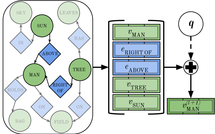
Figure 2: C-GAT layer where we illustrate the update of vertex MAN by combining the features of all incoming relations (and objects) through an attention mechanism. The attention scores are conditioned on the external query vector $\bm{q}$.

In Figure 2, a C-GAT layer is applied to an input scene graph $\mathcal{G}$ and conditioned on a query vector $\bm{q}$, i.e. the decoder state. We illustrate the update of vertex $v_{\text{man}}\in\mathcal{V}$ using features from its neighbourhood $\mathcal{N}(v_{\text{man}})$. The self-relation is assumed to always be present and for readability is not shown. Neighbour nodes’ features are combined with an MLP attention mechanism (Bahdanau et al., 2014) and scores are computed using query $\bm{q}$.

As described in Section 2.3, neighbours of an object vertex $v_{i}\in\mathcal{V}$ in a scene graph only include relation vertices. To include neighbour object features as well as relation features, we collect features for all $v_{j}\in\mathcal{N}_{\text{obj}}(v_{i})$, defined as nodes accessible by all relation vertices $v_{r}$ such that $\{v_{i}\leftarrow v_{r},v_{r}\leftarrow v_{j}\}\in\mathcal{E}$.

4 Model Setup

In this section, we first introduce image captioning models that do not explicitly use relation features (Section 4.1) and contrast them with those that use explicit relation features (Section 4.2).

4.1 Baseline Image Captioning (IC)

Bottom-Up Top-Down (BUTD)

The bottom-up top-down (BUTD; Anderson et al., 2018) model consists of a Faster R-CNN image encoder  (Ren et al., 2015) that computes object proposal features for an input image, and a 2-layer LSTM language model decoder with a MLP attention mechanism over the object features that generates a caption for the image (Hochreiter and Schmidhuber, 1997; Bahdanau et al., 2014). We denote the set of object features $\mathbf{X}\in\mathbb{R}^{n\times d}$, where $n$ is the number of objects in the image and $d$ the features dimensionality. The 2-layer LSTM is designed so that the first layer is used to compute an attention over the image features and the second layer is used to generate the captions’ tokens. LSTM states at time step $t$ are denoted as $\bm{h}_{1}^{(t)}$ and $\bm{h}_{2}^{(t)}$ for layer 1 and 2, respectively. The hidden state of LSTM₁ is used to derive an attention over image features:

$$\bm{x}^{(t)}=\mathit{Att}(\mathbf{X},\bm{h}_{1}^{(t)}),$$ (1)

where $\bm{x}^{(t)}\in\mathbb{R}^{d}$ is the output of the attention layer and denotes the image features used at time step $t$. Update rules for each LSTM layer are defined by:

$$\bm{h}_{1}^{(t)} =\text{LSTM}_{1}([\bm{h}_{2}^{(t-1)};\bm{w}^{(t-1)};\bar{\mathbf{X}}],\quad\bm{h}_{1}^{(t-1)}),$$ (2)

$$\bm{h}_{2}^{(t)} =\text{LSTM}_{2}([\bm{h}_{1}^{(t)};\bm{x}^{(t)}],\quad\bm{h}_{2}^{(t-1)}),$$ (3)

where $\bm{w}^{(t-1)}$ is the embedding of the previously generated word, and $\bar{\mathbf{X}}\in\mathbb{R}^{d}$ are the mean image features.

Next word probabilities are computed using a softmax over the vocabulary and parameterised by a linear projection of the hidden state of LSTM₂: $p(w^{(t)}=k|\bm{w}^{(1):(t-1)})\propto\exp(\bm{W}\bm{h}_{2}^{(t)})$.

4.2 Relation-aware Image Captioning (RIC)

We now describe models that incorporate explicit relation information into image captioning by using scene graphs as additional inputs.

We use the pretrained Iterative Message Passing model with a relation proposal network (Xu et al., 2017; Yang et al., 2018) to obtain scene graph features for all images. Scene graph features for an image are denoted $\mathbf{Y}\in\mathbb{R}^{(o+r)\times k}$, where $o$ is the number of objects, $r$ the number of relations between objects, and $k$ is the object/relation feature dimensionality.

We follow Wang et al. (2019) who have found that only using scene graph features led to poor results compared to using Faster R-CNN features only. Therefore, we propose to integrate scene graph features $\mathbf{Y}$ and Faster R-CNN object features $\mathbf{X}$ by experimenting with (i) using $\mathbf{Y}$ directly, applying a GAT layer on $\mathbf{Y}$, or applying a C-GAT layer on $\mathbf{Y}$ prior to feeding scene graph features into the decoder, and (ii) using a flat attention mechanism versus a hierarchical attention mechanism.

GAT over Scene Graphs

We propose a model that encodes the scene graph features $\mathbf{Y}$ with a standard GAT layer prior to using them in LSTM₂ in the decoder.

C-GAT over Scene Graphs

In this setup, we apply a C-GAT layer on scene graph features $\mathbf{Y}$ using the current decoder state $\mathbf{h}^{(t)}_{1}$ from LSTM₁ as the external context, and use the output of the C-GAT layer in LSTM₂ in the decoder.

Flat Attention

The flat attention (FA) consists of two separate attention heads, one over scene graph features $\mathbf{Y}$ and the other over Faster R-CNN features $\mathbf{X}$. We use two standard MLP attention mechanisms (Bahdanau et al., 2014), each using the hidden state from LSTM₁ as the query:

$$\bm{x}^{(t)}=\mathit{Att}_{x}(\mathbf{X},\bm{h}_{1}^{(t)}),$$

$$\bm{y}^{(t)}=\mathit{Att}_{y}(\mathbf{Y},\bm{h}_{1}^{(t)}).$$

Each LSTM layer is now defined as follows:

$$\bm{h}_{1}^{(t)} =\text{LSTM}_{1}([\bm{h}_{2}^{(t-1)};\bm{w}^{(t-1)};\bar{\mathbf{X}};\bar{\mathbf{Y}}],\bm{h}_{1}^{(t-1)}),$$

$$\bm{h}_{2}^{(t)} =\text{LSTM}_{2}([\bm{h}_{1}^{(t)};\bm{x}^{(t)};\bm{y}^{(t)}],\quad\bm{h}_{2}^{(t-1)}),$$ (4)

where $\bm{x}^{(t)}$ and $\bm{y}^{(t)}$ are computed by the two attention heads $Att_{x}$ and $Att_{y}$, respectively, and $\bar{\mathbf{Y}}$ denote the mean scene graph features.

Hierarchical Attention

In a hierarchical attention (HA) mechanism the output of the first attention head is used as input to derive the attention of the second head. We again have two sets of inputs, scene graph features $\mathbf{Y}$ and Faster R-CNN object features $\mathbf{X}$. We experiment first using $\mathbf{Y}$ as input to the first head, and its output $\mathbf{y}^{(t)}$ as additional input to the second head:

$$\bm{y}^{(t)} =\mathit{Att}_{y}(\mathbf{Y},\bm{h}_{1}^{(t)}),$$

$$\bm{x}^{(t)} =\mathit{Att}_{x}(\mathbf{X},[\bm{h}_{1}^{(t)};\bm{y}^{(t)}]).$$ (5)

This setup is similar to the cascade attention from Wang et al. (2019). We also try using $\mathbf{X}$ as input to the first head, and the first head’s output $\mathbf{x}^{(t)}$ as additional input to the second head:

$$\bm{x}^{(t)} =\mathit{Att}_{x}(\mathbf{X},\bm{h}_{1}^{(t)}).$$

$$\bm{y}^{(t)} =\mathit{Att}_{y}(\mathbf{Y},[\bm{h}_{1}^{(t)};\bm{x}^{(t)}]).$$ (6)

In both cases, the hidden states for LSTM₁ and LSTM₂ are computed as in Equation 4.

5 Experimental Setup and Results

We compare our models with the following external baselines with no access to scene graphs: (1) the adaptive attention model Add-Att which determines at each decoder time step how much of the visual features should be used (Lu et al., 2017); (2) the Neural Baby Talk model NBT generates a sentence with gaps and fills the gaps using detected object labels (Lu et al., 2018); (3) and the BUTD model (Anderson et al., 2018) described in Section 4.1.

We also compare with the following baselines that use scene graphs: (1) The “Know more, say less” model KMSL extracts features for objects and relations based on the scene graph, which are passed through two attention heads and finally combined using a flat attention head (Li and Jiang, 2019); and (2) the Cascade model (Wang et al., 2019) which is similar to our hierarchical attention model with a GAT layer, but that instead uses a relational graph convolutional network (Marcheggiani et al., 2017).

We do not discuss model variants/results that are trained with an additional reinforcement learning step (Rennie et al., 2017; Yang et al., 2019) and only compare single model results, since training and performing inference with such models is very costly and orthogonal to our research questions.

Our proposed models are: flat attention (FA), hierarchical attention with scene graph first (HA-SG) following Equation 5, hierarchical attention with objects detected first (HA-IM) following Equation 6, HA-SG with graph attention network (HA-SG +GAT), and HA-SG with conditional graph attention (HA-SG +C-GAT). We choose the last two variants to extend HA-SG following the setup used by (Wang et al., 2019).

We evaluate captions generated by different models by investigating their SPICE scores Anderson et al. (2016), i.e. an F1 based semantic captioning evaluation metric computed over scene graphs. It uses the semantic structure of the scene graph to compute scores over several dimensions (object, relation, attribute, colour, count, and size).

We use the MSCOCO karpathy split (Lin et al., 2014; Karpathy and Fei-Fei, 2015) which has 5k images each in validation and test sets, and we use the remaining 113k images for training. We build a vocabulary based on all words in the train split that occur at least 5 times. We use MSCOCO evaluation scripts (Lin et al., 2014) and report BLEU4 (B4; Papineni et al., 2002), CIDEr (C; Vedantam et al., 2015), ROUGE-L (R; Lin, 2004), and SPICE (S; Anderson et al., 2016). See Appendix A for extra information on our implementation and training procedures.

	B4		C	R	S
Add-Att${*^{\dagger}}$	33.2		108.5	—	—
NBT†	34.7		107.2	—	20.1
BUTD†	36.2		113.5	56.4	20.3
BUTD	34.8		109.2	55.7	20.0
Cascade†	34.1		108.6	55.9	20.3
KMSL†	33.8		110.3	54.9	19.8
FA	33.7		102.5	54.7	18.8
HA-IM	35.7		109.9	55.9	19.9
HA-SG	35.0		109.1	55.7	19.8
+ GAT	34.7		106.4	55.4	19.4
+ C-GAT	35.5		109.9	56.0	19.8

Table 1: Results on the MSCOCO test set, with models selected on the validation set (karpathy splits). Models in the upper section do not use scene graphs, while those in the bottom section do. All models are trained to convergence for a maximum of 50 epochs. Metrics reported are: BLEU-4 (B4), CIDEr (C), ROUGE-L (R), and SPICE (S). See Section 5 for details on all models and acronyms. We bold-face the best and underscore the second-best scores per metric (models that use scene graph). ^∗ Model uses features from last convolutional layer in CNN, i.e. no Faster R-CNN features. ^† Results reported in the authors’ original papers.

5.1 Image Captioning without Relational Features

Our re-implementation of the BUTD baseline scores slightly worse compared to the results reported by Anderson et al. (2018). This difference can be attributed to the Faster R-CNN features used, i.e. we always use 36 objects per image whereas Anderson et al. (2018) use a variable number of objects per image (i.e. 10 to 100), and there are other smaller differences in their training procedure. Since all our models use these settings, in further experiments we compare to our implementation of the BUTD baseline.

5.2 Image Captioning with relational features

We notice that the KMSL model by Li and Jiang (2019) slightly outperforms the other models according to CIDEr, while it performs worse in all other metrics. Li and Jiang (2019) found performance increases when restricting the number of relations and report scores using this restriction, whereas we decided to use the full set of relations to test the effect of scene graph quality (see Section 5.4). Furthermore, the features used in the KMSL model are not directly extracted from the SGG model as is the case for the other models, but an additional architecture is used for computing stronger features.

Flat vs. Hierarchical attention

According to Table 1, FA performs worse not only compared to HA models, but also compared to other baselines.

The HA model using Faster R-CNN object features in the first head, i.e. HA-IM setup, performs better than using the scene graph features first, i.e. HA-SG setup. We hypothesise that this difference comes from the additional guidance from $\mathbf{x}^{(t)}$ helping with a better attention selection over possibly more noisy features present in $\mathbf{Y}$.

Additional GNN updates

Directly using a GAT layer over scene graph features negatively impacts model performance. Comparing these results to the related Cascade model from Wang et al. (2019), we hypothesise that the R-GCN architecture works better in this setting, although compared to other models it still has lower scores according to most metrics. The reason may be that the Cascade model by Wang et al. (2019) was undertrained or could have used better hyperparameters, as indicated by our BUTD baseline performing comparably or better than their strongest model.

Combining a C-GAT layer on the decoder improves overall results according to most metrics, though by a small margin. This suggests that using additional GNNs in the context of image captioning have a positive effect. Furthermore, graph features learned using C-GAT always outperform standard GAT, which coincides with our intuition that taking the current decoder hidden context into consideration can improve graph features.

5.3 SPICE breakdown

	All		Obj		Rel
BUTD	19.8		36.0		5.2
FA	18.5		34.7		5.0
HA-IM	19.5		35.9		5.2
HA-SG	19.5		35.9		5.3
+ GAT	19.2		35.5		5.6
+ C-GAT	19.4		35.8		5.3

Table 2: Breakdown of overall SPICE scores (All) into object (Obj) and relation (Rel) F1 scores. See Section 5 for details on all models and acronyms. We bold-face the best overall scores and underline the best scores obtained by our models.

In our analysis, in addition to the overall SPICE F1 score for an entire caption, we break it down into scores over objects and over relations. This allows us to investigate how models are better or worse on describing objects and relations independently. These results, computed for the validation split, are shown in Table 2.

When we look at individual scores for objects and relations, we notice a small and consistent gain in relation F1 by using scene graphs independently of the attention architecture or other design choices, but also observe lower object F1 scores with respect to the BUTD baseline. When object and relation scores are combined into a single F1 measure, it results in worse overall scores suggesting that the small increase in the relation scores is not sufficient to have a positive impact on captioning insofar.

5.4 Scene Graph Quality

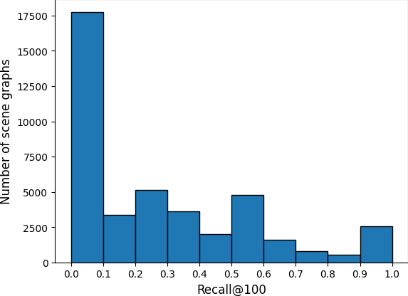
Figure 3: Distribution of the scores for the scene graphs in the validation split of the VG-COCO dataset.

	SPICE						Captioning
	All		Obj		Rel		B4		C	R
BUTD	19.8		36.0		5.0		35.4		109.8	56.0
FA	18.5		34.9		4.8		33.2		103.6	54.8
HA-IM	19.6		36.0		5.2		35.0		110.8	55.7
HA-SG	19.8		36.2		5.5		35.7		111.0	56.0
+ GAT	19.4		35.5		5.6		35.0		108.3	55.6
+ C-GAT	19.5		35.8		5.2		35.7		110.4	56.0

(a) Full VG-COCO dataset

SPICE						Captioning
All		Obj		Rel		B4		C	R
19.5		35.6		4.7		34.0		109.2	55.2
18.2		34.9		4.4		32.4		102.7	54.3
19.5		36.0		5.2		34.3		111.7	55.5
19.6		36.0		5.0		34.6		110.3	55.4
19.5		35.7		5.7		34.8		109.5	55.4
19.5		35.7		5.1		34.8		109.9	55.7

(b) Low VG-COCO dataset

	SPICE						Captioning
	All		Obj		Rel		B4		C	R
BUTD	20.5		37.0		5.5		38.4		117.5	57.1
FA	18.8		35.0		5.3		34.6		111.1	55.1
HA-IM	19.8		36.2		5.3		36.2		115.1	55.3
HA-SG	19.6		35.9		5.4		37.0		114.4	56.3
+ GAT	19.4		35.8		5.7		36.2		112.7	56.0
+ C-GAT	19.5		36.0		5.1		37.6		116.4	56.1

(c) Average VG-COCO dataset

SPICE						Captioning
All		Obj		Rel		B4		C	R
20.9		36.8		5.1		37.2		126.5	57.0
19.8		35.3		5.6		35.9		117.4	56.6
20.3		36.2		5.8		36.2		124.1	56.8
20.9		37.1		6.0		38.1		129.8	57.6
19.7		35.3		5.9		36.2		123.6	57.1
20.8		36.6		6.0		37.2		127.3	56.9

(d) High VG-COCO dataset

Table 3: SPICE breakdown and captioning metrics for images in VG-COCO validation split. Results for the full VG-COCO, and for subsets of images collected according to the quality of their corresponding predicted scene graphs: low, average, and high. See Sections 5 for details on all models and acronyms. Metrics reported are: overall SPICE F1 score (All), object (Obj) and relation (Rel) F1 score components, BLEU-4 (B4), CIDEr (C), and ROUGE-L (R). We bold-face the best and underline the second-best overall scores per metric and per data subset.

Since scene graph features are generated with a pretrained SGG model, we expect them to introduce a considerable amount of noise into the model. In this section, we investigate the effect that the quality of the scene graph has on the quality of captions.

VG-COCO

In this set of experiments, we need images with both captions and scene graph annotations. Thus, we use a subset of MSCOCO which overlaps with Visual Genome (Krishna et al., 2017), using captions from the former and scene graphs from the latter. We refer to this dataset as VG-COCO, as similarly done by Li and Jiang (2019). We compute scores for each scene graph predicted by the Iterative Message Passing model using the common SGDet recall@100 as defined by Yang et al. (2018). SGDet recall@100 is computed by using the 100 highest scoring triplets among all triplets predicted by the model, and reporting the percentage of gold-standard triplets. The distribution of scores across images (Figure 3) shows that most scene graphs have extremely low scores close to zero, thus containing a lot of noise.

We separate images in the VG-COCO validation set in three groups: low (R $<33\%$), average ($33\%\leq$ R $<67\%$), and high scoring graphs ($67\%\leq$ R), where R is SGDet recall@100. For each set of images in each of these groups, we compute captioning metrics and also report a SPICE breakdown in Table 3.

Effect of scene graph quality

Due to the imbalance in scene graph quality, the low, average, and high quality subsets have around 1000, 500, and 200 images, respectively. By reporting results for the BUTD baseline, we show the performance a strong baseline obtains on the same set of images.

In Table 3b, scores across all metrics are similar and only model FA performs clearly worse than others. Though the BUTD baseline never performs best, it is often not more than a point behind the best performing model (except for CIDEr where it is 2.5 points lower compared to HA-IM).

When comparing Table 3b to Table 3c, we observe that all models tend to increase scores, and that BUTD tends to perform best overall. In Table 3d, we see an increase in the difference between the baseline and our best models according to all metrics. All these gains are very promising and suggest that when we have high quality scene graphs, we can expect a consistent positive transfer into image captioning models. However, the overall SPICE score is the highest for both BUTD and HA-SG, while BUTD has lower scores for objects and relations F-measure. That suggests that other components part of SPICE were worsened with the addition of scene graphs. Since this is not the focus of this paper, we did not investigate this further and leave that for future work.

Overall, these results show that indiscriminately using scene graphs from pretrained SGG models downstream on image captioning can be harmful because of the amount of noise present in these scene graphs. However, when this noise is smaller and the scene graphs of higher quality, our findings together suggest that scene graphs can be useful in image captioning models.

Ground-truth graphs

Finally, we also conduct a small-scale experiment using ground-truth scene graphs and evaluate how using these instead of predicted scene graphs at inference time impacts models, which can be found in Appendix B.

Qualitative Results

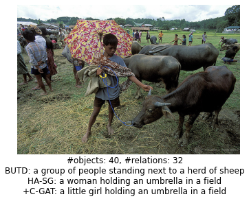
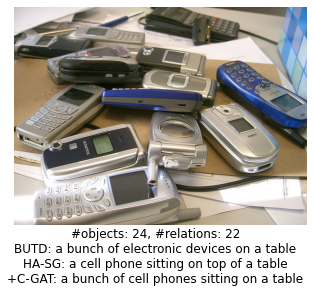
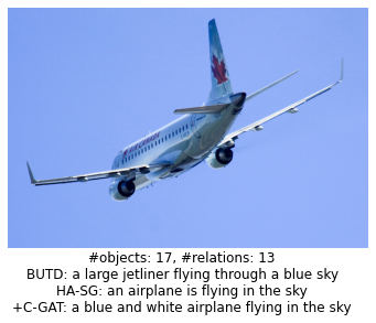
Figure 4: Images, captions and ground-truth number of objects and relations for high scoring scene graph.

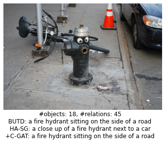
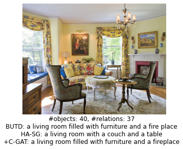
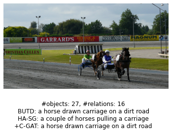
Figure 5: Images, captions and ground-truth number of objects and relations for low scoring scene graph.

Here, we try to determine if there is a clear difference in the difficulty in captioning images in low, average, and high quality sets, which might help explain the result in Table 3. In Figures 4 and 5 we show some images for the low and high scoring graphs, respectively. At a first glance, images from both sets appear equally cluttered with objects (i.e., which we hypothesise should correlate with the image being harder to describe). Furthermore, for both low and high scoring scene graphs, the average number of objects and relations is 23 and 22 respectively. However, we note that even scene graphs in the high quality set often include tiny objects and details, e.g. the image in the right of Figure 4 shows a single aircraft, but there are 17 annotated objects describing components such as wings, windows, etc.

6 Conclusions and Future Work

In this work, we investigate the impact scene graphs have on image captioning. We introduced conditional graph attention (C-GAT)networks and applied it to image captioning, and report promising results (Table 1). Overall, we found that improvements in captioning when using scene graphs generated with publicly available SGG models are minor. We observe a very small increase in the ability to describe relations as measured by relation SPICE F-scores, however, this is associated with models producing worse overall descriptions and producing lower object SPICE F-scores.

In an in-depth analysis, we found that the predicted scene graphs contain a large amount of noise which harms the captioning process. When this noise is reduced, large gains can be achieved across all image captioning metrics, e.g. 3.3 CIDEr points in the high VG-COCO split (Table 3d). This indicates that with further research and improved scene graph generation models, we will likely be able to observe consistent gains in image captioning and possibly other tasks by leveraging silver-standard scene graphs.

Future work

In further research, we will conduct an in-depth analysis of our proposed conditional graph attention to determine what tasks other than image captioning we can apply it to. We envision using it for visual question-answering also with generated scene graphs, and on syntax-aware neural machine translation (Bastings et al., 2017), fake news detection (Monti et al., 2019), and question answering (Zhang et al., 2018).

In a focused qualitative analysis, we found that the scene graphs represent objects and relations in images sometimes with great detail. We plan to investigate how to account for such highly detailed objects/relations in the context of image captioning. Finally, we will look into a method to use predicted scene graphs selectively according to their estimated quality, possibly selecting the best graph between those generated by different SGG models.

Appendix A Implementation Details

All our models are trained until convergence using early stopping with a patience of 20 epochs and a maximum of 50 epochs. We use the Adamax optimizer (Kingma and Ba, 2014) with an initial learning rate of 0.002, which we decay with a factor of 0.8 after 8 epochs without improvements on the validation set. Dropout regularisation with a probability of $50\%$ is applied on word embeddings and on the hidden state of the second LSTM layer $h_{2}^{(t)}$ before it is projected to compute the next word probabilities. We use a beam size of 5 during evaluation. All hidden layers and embedding sizes are set to 1024. Models are all trained on a single 12GB NVIDIA GPU.

We use a fixed number of $n=36$ objects extracted with our pretrained Faster R-CNN. The number of objects and relations extracted with the pretrained Iterative Message Passing model varies according to the input image, i.e. a maximum of $o=100$ objects and of $r=2500$ relations.

Appendix B Using Ground-Truth Graphs

	SPICE						Captioning
	All		Obj		Rel		B4		C	R
FA	18.3		34.3		5.3		30.5		95.8	53.1
HA-IM	19.0		35.2		4.8		33.5		106.0	54.8
HA-SG	18.8		34.7		4.9		32.9		104.5	54.3
+ GAT	18.6		34.7		5.2		32.5		100.9	53.9
+ C-GAT	18.9		34.8		5.1		33.6		104.3	54.5

Table 4: Results for the full VG-COCO validation set using features extracted for ground-truth scene graphs. Models and acronyms are described in Sections 5. Metrics reported are: the overall SPICE F1 score (All) and its object (Obj) and relation (Rel) F1 score components, BLEU-4 (B4), CIDEr (C), and ROUGE-L (R). We bold-face the best and underline the second-best overall scores per metric.

In this small-scale experiment, we generate features for ground-truth scene graphs to determine if more a positive transfer can be achieved on image captioning models. For the VG-COCO dataset, we take all the ground-truth object and relation boxes and pass these through the pretrained Iterative Message Passing (IMP) model, instead of the RPN and RelPN proposed boxes. This is the same pretrained (IMP) model used in the other experiments.

Wang et al. (2019) also did a similar experiment, however, they also trained their models using features from gold-standard scene graphs, whereas we only use them to evaluate models previously trained on predicted scene graph features. In Table 4 we show that when using ground-truth scene graphs results are worse than those obtained using predicted ones (Table 3a). One obvious explanation is the mismatch between training and testing data, with regards to quality and number of features. Models are trained on the predicted scene graphs, which have an average of 34 object and 48 relation features per image (probably noisy, as seen in Section 5.4), whereas ground-truth graphs have an average of 21 objects and 18 relations per image.

References

- Anderson et al. (2016) Peter Anderson, Basura Fernando, Mark Johnson, and Stephen Gould. 2016. Spice: Semantic propositional image caption evaluation. In Computer Vision – ECCV 2016, pages 382–398, Cham. Springer International Publishing.
- Anderson et al. (2018) Peter Anderson, Xiaodong He, Chris Buehler, Damien Teney, Mark Johnson, Stephen Gould, and Lei Zhang. 2018. Bottom-up and top-down attention for image captioning and visual question answering. In The IEEE Conference on Computer Vision and Pattern Recognition (CVPR).
- Bahdanau et al. (2014) Dzmitry Bahdanau, Kyunghyun Cho, and Yoshua Bengio. 2014. Neural machine translation by jointly learning to align and translate. arXiv preprint arXiv:1409.0473.
- Bastings et al. (2017) Joost Bastings, Ivan Titov, Wilker Aziz, Diego Marcheggiani, and Khalil Sima’an. 2017. Graph convolutional encoders for syntax-aware neural machine translation. In Proceedings of the 2017 Conference on Empirical Methods in Natural Language Processing, pages 1957–1967, Copenhagen, Denmark. Association for Computational Linguistics.
- Battaglia et al. (2018) Peter W Battaglia, Jessica B Hamrick, Victor Bapst, Alvaro Sanchez-Gonzalez, Vinicius Zambaldi, Mateusz Malinowski, Andrea Tacchetti, David Raposo, Adam Santoro, Ryan Faulkner, et al. 2018. Relational inductive biases, deep learning, and graph networks. arXiv preprint arXiv:1806.01261.
- Girshick (2015) Ross Girshick. 2015. Fast R-CNN. In Proceedings of the 2015 IEEE International Conference on Computer Vision (ICCV), ICCV ’15, page 1440–1448, USA. IEEE Computer Society.
- Girshick et al. (2014) Ross Girshick, Jeff Donahue, Trevor Darrell, and Jitendra Malik. 2014. Rich feature hierarchies for accurate object detection and semantic segmentation. In Proceedings of the 2014 IEEE Conference on Computer Vision and Pattern Recognition, CVPR ’14, page 580–587, USA. IEEE Computer Society.
- He et al. (2016) Kaiming He, Xiangyu Zhang, Shaoqing Ren, and Jian Sun. 2016. Deep residual learning for image recognition. In Proceedings of the IEEE Conference on Computer Vision and Pattern Recognition, pages 770–778.
- Hochreiter and Schmidhuber (1997) Sepp Hochreiter and Jürgen Schmidhuber. 1997. Long short-term memory. Neural computation, 9(8):1735–1780.
- Johnson et al. (2018) Justin Johnson, Agrim Gupta, and Li Fei-Fei. 2018. Image generation from scene graphs. In Proceedings of the IEEE Conference on Computer Vision and Pattern Recognition, pages 1219–1228.
- Johnson et al. (2017) Justin Johnson, Bharath Hariharan, Laurens van der Maaten, Li Fei-Fei, C. Lawrence Zitnick, and Ross Girshick. 2017. CLEVR: A Diagnostic Dataset for Compositional Language and Elementary Visual Reasoning. In The IEEE Conference on Computer Vision and Pattern Recognition (CVPR).
- Johnson et al. (2015) Justin Johnson, Ranjay Krishna, Michael Stark, Li-Jia Li, David Shamma, Michael Bernstein, and Li Fei-Fei. 2015. Image retrieval using scene graphs. In Proceedings of the IEEE conference on computer vision and pattern recognition, pages 3668–3678.
- Karpathy and Fei-Fei (2015) Andrej Karpathy and Li Fei-Fei. 2015. Deep visual-semantic alignments for generating image descriptions. In Proceedings of the IEEE conference on computer vision and pattern recognition, pages 3128–3137.
- Kingma and Ba (2014) Diederik P Kingma and Jimmy Ba. 2014. Adam: A method for stochastic optimization. arXiv preprint arXiv:1412.6980.
- Knyazev et al. (2020) Boris Knyazev, Harm de Vries, Cătălina Cangea, Graham W Taylor, Aaron Courville, and Eugene Belilovsky. 2020. Graph density-aware losses for novel compositions in scene graph generation. arXiv preprint arXiv:2005.08230.
- Krishna et al. (2017) Ranjay Krishna, Yuke Zhu, Oliver Groth, Justin Johnson, Kenji Hata, Joshua Kravitz, Stephanie Chen, Yannis Kalantidis, Li-Jia Li, David A. Shamma, and et al. 2017. Visual genome: Connecting language and vision using crowdsourced dense image annotations. International Journal of Computer Vision, 123(1):32–73.
- Li et al. (2019) Guang Li, Linchao Zhu, Ping Liu, and Yi Yang. 2019. Entangled transformer for image captioning. In Proceedings of the IEEE/CVF International Conference on Computer Vision (ICCV).
- Li and Jiang (2019) X. Li and S. Jiang. 2019. Know more say less: Image captioning based on scene graphs. IEEE Transactions on Multimedia, 21(8):2117–2130.
- Li et al. (2018) Yikang Li, Wanli Ouyang, Bolei Zhou, Jianping Shi, Chao Zhang, and Xiaogang Wang. 2018. Factorizable net: An efficient subgraph-based framework for scene graph generation. In Proceedings of the European Conference on Computer Vision (ECCV), pages 335–351.
- Lin (2004) Chin-Yew Lin. 2004. ROUGE: A package for automatic evaluation of summaries. In Text Summarization Branches Out, pages 74–81, Barcelona, Spain. Association for Computational Linguistics.
- Lin et al. (2014) Tsung-Yi Lin, Michael Maire, Serge Belongie, James Hays, Pietro Perona, Deva Ramanan, Piotr Dollár, and C Lawrence Zitnick. 2014. Microsoft coco: Common objects in context. In European conference on computer vision, pages 740–755. Springer.
- Lu et al. (2017) Jiasen Lu, Caiming Xiong, Devi Parikh, and Richard Socher. 2017. Knowing when to look: Adaptive attention via a visual sentinel for image captioning. In The IEEE Conference on Computer Vision and Pattern Recognition (CVPR).
- Lu et al. (2018) Jiasen Lu, Jianwei Yang, Dhruv Batra, and Devi Parikh. 2018. Neural baby talk. In Proceedings of the IEEE conference on computer vision and pattern recognition, pages 7219–7228.
- Marcheggiani et al. (2017) Diego Marcheggiani, Anton Frolov, and Ivan Titov. 2017. A simple and accurate syntax-agnostic neural model for dependency-based semantic role labeling. In Proceedings of the 21st Conference on Computational Natural Language Learning (CoNLL 2017), pages 411–420, Vancouver, Canada. Association for Computational Linguistics.
- Monti et al. (2019) Federico Monti, Fabrizio Frasca, Davide Eynard, Damon Mannion, and Michael M Bronstein. 2019. Fake news detection on social media using geometric deep learning. arXiv preprint arXiv:1902.06673.
- Papineni et al. (2002) Kishore Papineni, Salim Roukos, Todd Ward, and Wei-Jing Zhu. 2002. Bleu: A method for automatic evaluation of machine translation. In Proceedings of the 40th Annual Meeting on Association for Computational Linguistics, ACL ’02, pages 311–318, Stroudsburg, PA, USA. Association for Computational Linguistics.
- Ren et al. (2015) Shaoqing Ren, Kaiming He, Ross Girshick, and Jian Sun. 2015. Faster R-CNN: Towards real-time object detection with region proposal networks. In Advances in neural information processing systems, pages 91–99.
- Rennie et al. (2017) Steven J. Rennie, Etienne Marcheret, Youssef Mroueh, Jerret Ross, and Vaibhava Goel. 2017. Self-critical sequence training for image captioning. In The IEEE Conference on Computer Vision and Pattern Recognition (CVPR).
- Vaswani et al. (2017) Ashish Vaswani, Noam Shazeer, Niki Parmar, Jakob Uszkoreit, Llion Jones, Aidan N Gomez, Łukasz Kaiser, and Illia Polosukhin. 2017. Attention is all you need. In Advances in neural information processing systems, pages 5998–6008.
- Vedantam et al. (2015) Ramakrishna Vedantam, C. Lawrence Zitnick, and Devi Parikh. 2015. Cider: Consensus-based image description evaluation. In The IEEE Conference on Computer Vision and Pattern Recognition (CVPR).
- Veličković et al. (2018) Petar Veličković, Guillem Cucurull, Arantxa Casanova, Adriana Romero, Pietro Liò, and Yoshua Bengio. 2018. Graph attention networks. In International Conference on Learning Representations.
- Wang et al. (2019) Dalin Wang, Daniel Beck, and Trevor Cohn. 2019. On the role of scene graphs in image captioning. In Proceedings of the Beyond Vision and LANguage: inTEgrating Real-world kNowledge (LANTERN), pages 29–34, Hong Kong, China. Association for Computational Linguistics.
- Xu et al. (2017) Danfei Xu, Yuke Zhu, Christopher B Choy, and Li Fei-Fei. 2017. Scene graph generation by iterative message passing. In Proceedings of the IEEE Conference on Computer Vision and Pattern Recognition, pages 5410–5419.
- Yang et al. (2018) Jianwei Yang, Jiasen Lu, Stefan Lee, Dhruv Batra, and Devi Parikh. 2018. Graph R-CNN for scene graph generation. In Proceedings of the European Conference on Computer Vision (ECCV), pages 670–685.
- Yang et al. (2019) X. Yang, K. Tang, H. Zhang, and J. Cai. 2019. Auto-encoding scene graphs for image captioning. In 2019 IEEE/CVF Conference on Computer Vision and Pattern Recognition (CVPR), pages 10677–10686.
- Yu et al. (2019a) J. Yu, J. Li, Z. Yu, and Q. Huang. 2019a. Multimodal transformer with multi-view visual representation for image captioning. IEEE Transactions on Circuits and Systems for Video Technology, pages 1–1.
- Yu et al. (2019b) J. Yu, J. Li, Z. Yu, and Q. Huang. 2019b. Multimodal transformer with multi-view visual representation for image captioning. IEEE Transactions on Circuits and Systems for Video Technology, pages 1–1.
- Zellers et al. (2018) Rowan Zellers, Mark Yatskar, Sam Thomson, and Yejin Choi. 2018. Neural motifs: Scene graph parsing with global context. In Conference on Computer Vision and Pattern Recognition.
- Zhang et al. (2018) Yuyu Zhang, Hanjun Dai, Zornitsa Kozareva, Alexander J Smola, and Le Song. 2018. Variational reasoning for question answering with knowledge graph. In Thirty-Second AAAI Conference on Artificial Intelligence.