Dynamical Entanglement

Abstract

Unlike the entanglement of quantum states, very little is known about the entanglement of bipartite channels, called dynamical entanglement. Here we work with the partial transpose of a superchannel, and use it to define computable measures of dynamical entanglement, such as the negativity. We show that a version of it, the max-logarithmic negativity, represents the exact asymptotic dynamical entanglement cost. We discover a family of dynamical entanglement measures that provide necessary and sufficient conditions for bipartite channel simulation under local operations and classical communication and under operations with positive partial transpose.

Introduction.

Quantum entanglement [1, 2] is universally regarded as the most important quantum phenomenon, signaling the definitive departure from classical physics [3]. Its importance ranges across different areas of physics, from quantum thermodynamics [4, 5, 6, 7, 8, 9, 10, 11, 12, 13, 14], to quantum field theory [15, 16, 17] and condensed matter [18, 19, 20]. In quantum information it is a resource in many protocols that cannot be implemented in classical theory, such as quantum teleportation [21], dense coding [22], and quantum key distribution [23].

An even more crucial aspect of physics is that all systems evolve. This is described by quantum channels [24, 25, 26]. Given the importance of entanglement, a natural question is how physical evolution interacts with it. For example, one can wonder how much entanglement a given evolution creates or consumes.

To this end, in this letter, which is a concise presentation of the most significant results of our previous work [27], we push entanglement out of its boundaries to the next level: from quantum states (static entanglement) to quantum channels (dynamical entanglement), filling an important gap in the literature (an independent work in this respect is Ref. [28]). Preliminary work was done in Refs. [29, 30, 31, 32, 33, 34, 35], but here we study the topic in utmost generality, using resource theories [36, 37, 38, 39, 40, 41, 42, 43, 44, 45]. With them, the idea of entanglement as a resource can be made precise. Resource theories have recently attracted considerable attention [43], producing plenty of important results in quantum information [1, 2, 13, 46, 47, 48, 49]. Resource theories are particularly meaningful whenever there is a restriction on the set of quantum operations that can be performed, usually coming from the physical constraints of a task an agent is trying to do [43].

Looking closely at the entanglement protocols mentioned above [21, 22], one notices that a state is converted into a particular channel [50, 51]. Thus, the need of a framework that goes beyond the conversion between static entangled resources is built in the very notion of entanglement as a resource. In other terms, we want to treat static and dynamical resources on the same grounds. We do so by phrasing entanglement theory as a resource theory of quantum processes [43, 52, 53, 54]. In this setting, the generic resource is a bipartite channel [55, 56], instead of a bipartite state.

In this letter, we start from the simulation of bipartite channels with local operations and classical communication (LOCC) [57, 58, 59], and we derive a family of convex dynamical entanglement measures that provide necessary and sufficient conditions for the LOCC-simulation of channels.

The key tool for the remainder of the letter is a generalization of partial transpose [60, 61]. This allows us to define superchannels with positive partial transpose (PPT) [62], which constitute the largest set of superoperations to manipulate dynamical entanglement, also encompassing the standard entanglement manipulations involving LOCC. In this setting, we define measures of dynamical entanglement that can be computed efficiently with semidefinite programs (SDPs). Specifically, one of them, the max-logarithmic negativity, quantifies the amount of static entanglement needed to simulate a channel using PPT superchannels.

Finally, with the same generalization of the partial transpose, we discover bound dynamical entanglement, whereby it is not possible to produce entanglement out of a class of channels—PPT channels [63, 64]—that generalize PPT states [60, 61].

Notation.

Physical systems are denoted by capital letters (e.g., $A$) with $AB$ meaning $A\otimes B$. Working on quantum channels, it is convenient to associate two subsystems $A_{0}$ and $A_{1}$ with every system $A$, referring, respectively, to the input and output of the resource. In the case of static resources, we take $A_{0}$ to be one-dimensional. A channel from $A_{0}$ to $A_{1}$ is indicated with a calligraphic letter $\mathcal{N}_{A}:=\mathcal{N}_{A_{0}\rightarrow A_{1}}$. Superchannels are denoted by capital Greek letters (e.g., $\Theta$), and the action of superchannels on channels by square brackets. Thus $\Theta_{A\rightarrow B}\left[\mathcal{N}_{A}\right]$ indicates the action of the superchannel $\Theta$ on the channel $\mathcal{N}_{A}$.

LOCC simulation of bipartite channels.

To manipulate dynamical resources, one needs quantum superchannels [65, 66], which are linear maps sending quantum channels to quantum channels in a complete sense, i.e., even when tensored with the identity superchannel. This means that if $\mathcal{N}_{RA}$ is a quantum channel, $\Theta_{A\rightarrow B}\left[\mathcal{N}_{RA}\right]$ is still a quantum channel, for any $R$. Superchannels can be all realized concretely with a preprocessing channel and a postprocessing channel, connected by a memory system [65, 66]. Specifically, an LOCC superchannel, used in LOCC simulation, consists of LOCC pre- and post-processing, and is represented in Fig. 1.

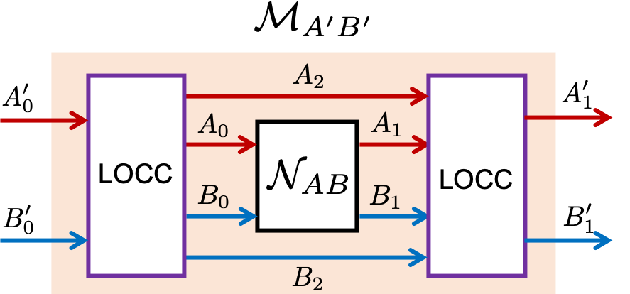
Figure 1: Simulation of the channel $\mathcal{M}_{A^{\prime}B^{\prime}}$ from the channel $\mathcal{N}_{AB}$ with an LOCC superchannel, which has LOCC pre- and postprocessing. Notice the presence of a memory system for each of the two parties ($A_{2}$ and $B_{2}$, respectively).

These superchannels are relevant when one is concerned with channel simulation in bipartite communication-type scenarios where only classical communication is allowed between the parties [57, 58] (e.g., in teleportation [21]).

Recall that with one qubit maximally entangled state (also known as an ebit), thanks to quantum teleportation [21], we can simulate a qubit noiseless channel from Alice to Bob using an LOCC scheme, and vice versa [50, 51]. Therefore one ebit—a static resource—is equivalent to a dynamical one: a qubit channel. With a pair of such channels at hand, from Alice to Bob and vice versa, we can LOCC-implement all bipartite channels between the two parties when they both have qubit systems. This means that such a pair of channels is the maximal resource. This is illustrated in Fig. 2(a).

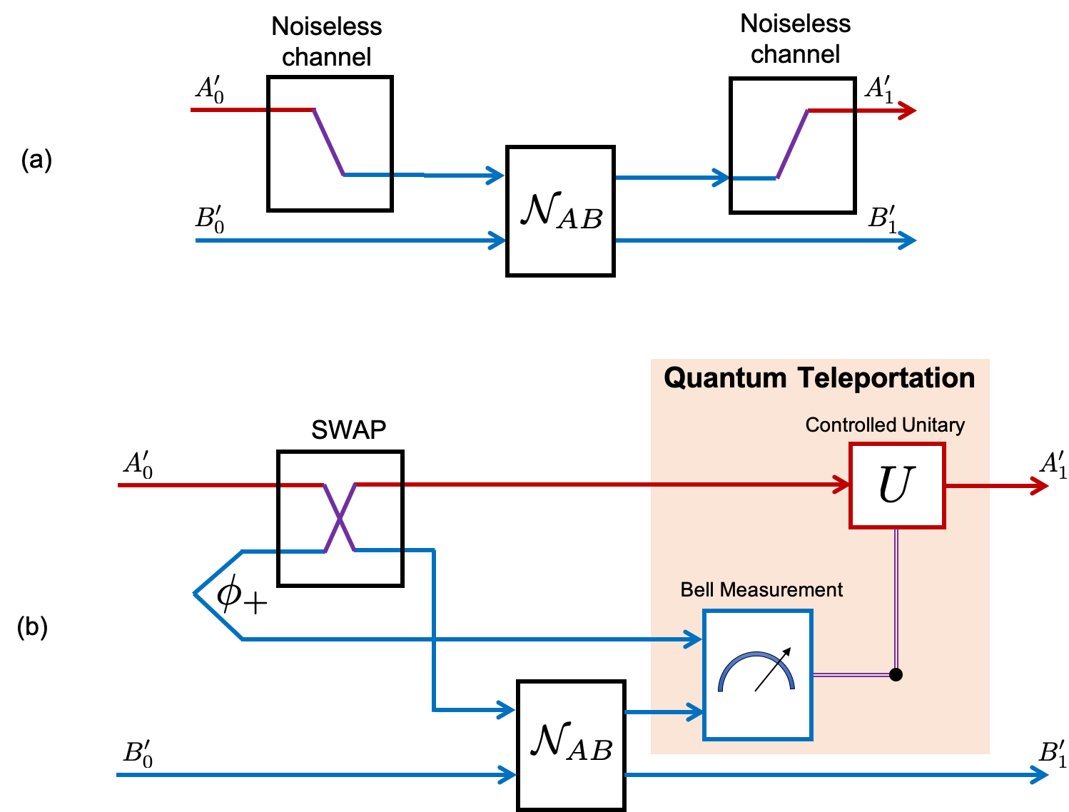
Figure 2: (a) Simulation of an arbitrary bipartite channel $\mathcal{N}_{A^{\prime}B^{\prime}}$ with two noiseless channels from Alice to Bob and vice versa. (b) Simulation of an arbitrary bipartite channel $\mathcal{N}_{A^{\prime}B^{\prime}}$ with the swap resource and an LOCC superchannel (the postprocessing is shaded in pink).

In Fig. 2(b) we show that in the same situation the swap operation is another maximal resource, equivalent to 2 ebits.

In entanglement theory, a function $f$ is a measure of dynamical entanglement if $f\left(\Theta\left[\mathcal{N}_{AB}\right]\right)\leq f\left(\mathcal{N}_{AB}\right)$, where $\Theta$ is an LOCC superchannel. It is conventional to assume that $f$ vanishes on all separable channels [67, 68, 63], which are regarded as the free resources in the theory of dynamical entanglement; but this is not essential.

The very definition of a measure of dynamical entanglement indicates that $f$ gives us a necessary condition for the simulation of channel $\mathcal{M}$ starting from channel $\mathcal{N}$ and using an LOCC superchannel $\Theta$. Indeed, if such a superchannel exists, namely $\mathcal{M}=\Theta\left[\mathcal{N}\right]$, then $f\left(\mathcal{M}\right)\leq f\left(\mathcal{N}\right)$. However, here we construct a family of convex measures of dynamical entanglement that also give us a sufficient condition for LOCC simulation. For any bipartite channels $\mathcal{P}$ and $\mathcal{N}$, define

$$E_{\mathcal{P}}\left(\mathcal{N}\right)=\sup_{\Theta\textrm{ LOCC}}\mathrm{Tr}\left[J^{\mathcal{P}}J^{\Theta\left[\mathcal{N}\right]}\right],$$ (1)

where $J$ denotes the Choi matrix of the channel in the superscript, and $\Theta$ is a generic LOCC superchannel. Note that these functions need not vanish on separable channels. It is possible to show that each function $E_{\mathcal{P}}$, with $\mathcal{P}$ ranging over all bipartite channels, can be computed using a conic linear program [27, subsection 3 C].

Theorem 1.

In the theory of dynamical entanglement, a channel $\mathcal{N}$ can be LOCC-converted into a channel $\mathcal{M}$ if and only if $E_{\mathcal{P}}\left(\mathcal{N}\right)\geq E_{\mathcal{P}}\left(\mathcal{M}\right)$ for every bipartite channel $\mathcal{P}$.

The proof is in Ref. [27, subsection 3 C]. Since we need to consider all bipartite channels $\mathcal{P}$, this family of measures of dynamical entanglement is not so practical to work with. Unfortunately, one cannot expect to find a finite family of such monotones, as shown in Ref. [69].

Given two channels $\mathcal{N}$ and $\mathcal{M}$, to determine if the former can be LOCC-converted into the latter, we can alternatively compute their conversion distance, defined following similar ideas to Ref. [70]:

$$d_{\mathrm{LOCC}}\left(\mathcal{N}\to\mathcal{M}\right)=\frac{1}{2}\inf_{\Theta\textrm{ LOCC}}\left\|\Theta\left[\mathcal{N}\right]-\mathcal{M}\right\|_{\diamond}.$$ (2)

If this distance is zero, we can convert $\mathcal{N}$ into $\mathcal{M}$ using a superchannel in the topological closure of LOCC superchannels [71]. Again, this distance can be calculated using a conic linear program [27, subsection 3 D], thanks to the results in Refs. [72, 54].

PPT superchannels.

In entanglement theory, one of the most practical tools to determine whether a state is entangled is the partial transpose [60, 61]. One defines PPT states as the bipartite states $\rho_{AB}$ such that $\mathcal{T}_{B}\left(\rho_{AB}\right)=\rho_{AB}^{T_{B}}$ is still a valid state, where $\mathcal{T}$ denotes the transpose map [60, 61]. Recall, however, that the set of PPT states is larger than the set of separable states, due to the existence of bound entangled states [73]. One then defines a PPT channel to be a bipartite channel $\mathcal{N}_{AB}$ such that, applying the transpose map on Bob’s input and output, we get another valid channel $\mathcal{N}_{AB}^{\Gamma}:=\mathcal{T}_{B_{1}}\circ\mathcal{N}_{AB}\circ\mathcal{T}_{B_{0}}$ [63, 64]. Note that the set of PPT channels is larger than the set of LOCC channels. It is not hard to show that PPT channels are also completely PPT preserving, for they preserve PPT states even when tensored with the identity channel [63, 64]. Finally, the Choi matrix of a PPT channel $\mathcal{N}_{AB}$ is such that $\left(J_{AB}^{\mathcal{N}}\right)^{T_{B}}\geq 0$. PPT states and operations can be regarded as free; therefore, anything that is not PPT—which we call NPT—will be a resource. For this reason, this resource theory is called the resource theory of NPT entanglement. As it often happens in resource theories, one considers a larger set of operations to get upper and lower bounds for the relevant figures of merit, especially when the interesting resource theory is mathematically hard to study, such as the LOCC theory [74, 75]. This is precisely why we study NPT entanglement.

Here we generalize partial transpose, defining the transpose supermap $\Upsilon$ as $\Upsilon\left[\mathcal{N}_{A}\right]=\mathcal{T}_{A_{1}}\circ\mathcal{N}_{A}\circ\mathcal{T}_{A_{0}}$. Note that the Choi matrix of $\Upsilon\left[\mathcal{N}_{A}\right]$ is the transpose of the Choi matrix of $\mathcal{N}_{A}$. In this way, PPT channels can be characterized in a similar way to PPT states: PPT channels are those bipartite channels such that $\Upsilon_{B}\left[\mathcal{N}_{AB}\right]$ is still a valid channel. Now we iterate the previous construction to define PPT superchannels.

Definition 2.

A superchannel $\Theta_{AB\rightarrow A^{\prime}B^{\prime}}$ is PPT if $\Theta_{AB\rightarrow A^{\prime}B^{\prime}}^{\Gamma}:=\Upsilon_{B^{\prime}}\circ\Theta_{AB\rightarrow A^{\prime}B^{\prime}}\circ\Upsilon_{B}$ is still a valid superchannel.

These superchannels enjoy some remarkable properties.

Lemma 3.

The following are equivalent:

1. $\Theta_{AB\rightarrow A^{\prime}B^{\prime}}$ is a PPT superchannel.

2. $\Theta_{AB\rightarrow A^{\prime}B^{\prime}}$ is completely PPT preserving.

3. $\left(\mathbf{J}_{ABA^{\prime}B^{\prime}}^{\Theta}\right)^{T_{BB^{\prime}}}\geq 0$, where $\mathbf{J}_{ABA^{\prime}B^{\prime}}^{\Theta}$ is the Choi matrix of the superchannel $\Theta$ [76, 77, 78, 79, 66].

A proof of this result can be found in Ref. [27, subsection 5 A]. Property 2 means that PPT superchannels preserve PPT channels in a complete sense. Property 3 tells us that PPT superchannels are the same objects that appeared in Ref. [62]. Despite the fairly simple condition defining PPT superchannels at the level of Choi matrices, we do not know if all of them can be realized with PPT pre- and postprocessing. When this happens, we call them restricted PPT superchannels. It is not hard to show that restricted PPT superchannels are indeed PPT superchannels in the sense of definition 2. Instead, we conjecture that the converse is not true, so we are really considering a larger set of superchannels. This is one of the main differences from a related work by Wang and Wilde [35]: there the authors study only restricted PPT superchannels, and they do not consider bipartite channels, but only one-way channels from Alice to Bob (or vice versa).

Our approach brings a lot of mathematical simplifications. For instance, if we replace LOCC with PPT in Eqs. (1) and (2), the NPT entanglement measures and the conversion distance become computable efficiently with SDPs (see Ref. [27, subsections 5 B and 5 C]). However, note that this family of NPT entanglement monotones will not provide a sufficient condition for the convertibility under LOCC superchannels.

New measures of dynamical entanglement.

Since PPT channels contain LOCC channels, PPT superchannels contain LOCC ones. Thus, measures of NPT dynamical entanglement (i.e., monotonic under PPT superchannels) are also measures of LOCC dynamical entanglement (i.e., monotonic under LOCC superchannels). As seen above, working with PPT superchannels is mathematically simpler. For this reason, focusing on the PPT-simulation of channels we obtain measures of LOCC dynamical entanglement that are easily computable.

The first example in this respect is the the negativity [80], defined for states as $N\left(\rho_{AB}\right)=\frac{\left\|\mathcal{T}_{B}\left(\rho_{AB}\right)\right\|_{1}-1}{2}$. The generalization to bipartite channels is straightforward: replace the trace norm with the diamond norm, and the transpose map $\mathcal{T}_{B}$ with the transpose supermap $\Upsilon_{B}$.

$$N\left(\mathcal{N}_{AB}\right)=\frac{\left\|\Upsilon_{B}\left[\mathcal{N}_{AB}\right]\right\|_{\diamond}-1}{2}.$$ (3)

Contextually, the logarithmic negativity is defined as

$$LN\left(\mathcal{N}_{AB}\right)=\log_{2}\left\|\Upsilon_{B}\left[\mathcal{N}_{AB}\right]\right\|_{\diamond}.$$ (4)

We prove that these are measures of dynamical entanglement that can be computed efficiently with an SDP (cf. Ref. [27, subsection 5 C]).

Now we introduce a new measure of NPT dynamical entanglement, called max-logarithmic negativity (MLN) (cf. [81]). It is a generalization of the notion of $\kappa$-entanglement introduced in [35]. The MLN is defined as

$$LN_{\max}\left(\mathcal{N}_{AB}\right)$$

$$:=\log_{2}\inf_{P_{AB}}\left\{\max\left\{\left\|P_{A_{0}B_{0}}\right\|_{\infty},\left\|P_{A_{0}B_{0}}^{T_{B_{0}}}\right\|_{\infty}\right\}\right\},$$ (5)

where $P_{AB}$ is a matrix subject to the constraints $-P_{AB}^{T_{B}}\leq\left(J_{AB}^{\mathcal{N}}\right)^{T_{B}}\leq P_{AB}^{T_{B}}$ and $P_{AB}\geq 0$. Here $P_{A_{0}B_{0}}$ denotes $\mathrm{Tr}_{A_{1}B_{1}}\left[P_{AB}\right]$. We can show that the MLN is an additive measure of dynamical entanglement, computable with an SDP (see Ref. [27, subsection 5 C]).

Despite its rather complicated definition, the MLN has a nice operational interpretation, which generalizes the results in Refs. [82, 35]. Consider the task of simulating $n$ parallel copies of the bipartite channel $\mathcal{N}_{AB}$ out of the maximally entangled state $\left|\phi_{m}^{+}\right\rangle_{A_{0}B_{0}}$ of Schmidt rank $m$ using PPT superchannels (which, in this case, take the form of PPT channels). Recall that $\left|\phi_{m}^{+}\right\rangle_{A_{0}B_{0}}$ is, up to a scaling factor 2, the maximal resource in the theory of entanglement for bipartite channels, as we noted above. We require that the conversion of $\left|\phi_{m}^{+}\right\rangle_{A_{0}B_{0}}$ into $\mathcal{N}_{AB}$ be exact for every $n$. We want to study the asymptotic entanglement cost of preparing $\mathcal{N}_{AB}$ according to this PPT protocol, viz. the minimum Schmidt rank of maximally entangled states consumed per copy of $\mathcal{N}_{AB}$ produced when $n\rightarrow+\infty$. Remarkably, we show that this cost is given precisely by the MLN. Clearly, the use of PPT superchannels is not so physically motivated, but it provides a simple lower bound to the more meaningful calculation of the entanglement cost under LOCC superchannels [82, 35].

Theorem 4.

The exact asymptotic NPT cost of a bipartite channel $\mathcal{N}_{AB}$ is $LN_{\max}\left(\mathcal{N}_{AB}\right)$.

A proof of this result can be found in Ref. [27, subsection 5 D]. We can prove that the MLN is an upper bound for another entanglement measure, the NPT entanglement generation power $E_{g}^{\mathrm{PPT}}$ [29, 52, 53, 54] (cf. Appendix A):

$$E_{g}^{\mathrm{PPT}}\left(\mathcal{N}_{AB}\right)\leq LN_{\max}\left(\mathcal{N}_{AB}\right).$$

Bound entanglement for bipartite channels.

Dual to the calculation of the cost of a bipartite channel, we have the distillation of ebits out of a dynamical resource. It is known that for some entangled static resources this is not possible: it is the phenomenon of bound entanglement [73], which occurs whenever we have a PPT entangled state.

Is it possible to distill ebits out $n$ copies of a PPT channel $\mathcal{N}_{AB}$? Now, when we have $n$ copies of a channel, the timing in which they are available becomes relevant: dynamical resources have a natural temporal ordering between input and output. Indeed, unlike states, they can also be composed in nonparallel ways, e.g., in sequence. Therefore, when manipulating dynamical resources, we also need to specify when and how they can be used (see also Refs. [53, 27]). This opens up the possibility of using adaptive schemes [32, 83, 33, 28]: if we have $n$ resources $\mathcal{N}_{1},\dots,\mathcal{N}_{n}$ that are available, respectively, at times $t_{1}\leq t_{2}\leq\dots\leq t_{n}$, the most general channel that can be simulated with these resources is given by a free $n$-comb [84, 76, 77, 85, 86, 87, 52, 53], depicted in Fig. 3 in the case of a PPT comb.

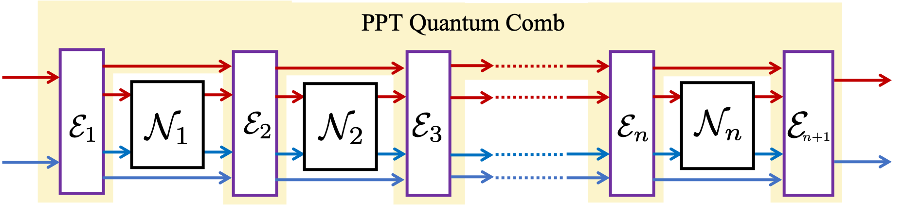
Figure 3: A PPT $n$-comb acts on $n$ bipartite channels $\mathcal{N}_{j}$, e.g., to distill ebits.

Specializing this idea to the case of dynamical entanglement, this amounts to considering an LOCC $n$-comb, where all the $n+1$ channels $\mathcal{E}_{1}$, …, $\mathcal{E}_{n+1}$ in Fig. 3 are LOCC. Then we plug the $n$ copies of $\mathcal{N}_{AB}$ into its $n$ slots.

Instead of LOCC combs, we consider PPT combs, which are defined as the combs for which the composition of channels $\mathcal{E}_{n+1}\circ\dots\circ\mathcal{E}_{1}$ in Fig. 3 is a PPT channel. This is equivalent to requiring that the Choi matrix of the $n$-comb [76, 77, 27] is the Choi matrix of a PPT channel. PPT combs will give us an upper bound on the amount of ebits generated in an LOCC procedure. However, again, we do not know if this implies that each channel $\mathcal{E}_{1}$, …, $\mathcal{E}_{n+1}$ is PPT, but we conjecture it is not the case.

By the mathematical properties of PPT combs and PPT channels, we can show that no ebits can be distilled out of PPT channels even with the most general adaptive PPT scheme (see Ref. [27, section 7]). Since this is an upper bound for LOCC adaptive schemes, we conclude that no entanglement distillation from PPT channels is possible under LOCC protocols either.

Theorem 5.

It is impossible to distill entangled ebits from PPT channels under any adaptive schemes in any resource theory of dynamical entanglement.

As a result, we find an example of a bound entangled POVM.

Example 6.

Recall that a POVM can be viewed as a quantum-to-classical channel. Let $\beta_{A_{0}B_{0}}$ be any PPT bound entangled state of a bipartite system $A_{0}B_{0}$, and consider the binary POVM $\left\{\beta_{A_{0}B_{0}},I_{A_{0}B_{0}}-\beta_{A_{0}B_{0}}\right\}$. Since both $\beta_{A_{0}B_{0}}$ and $I_{A_{0}B_{0}}-\beta_{A_{0}B_{0}}$ have positive partial transpose, it follows that this POVM is a PPT channel. As such, it cannot produce distillable entanglement. This means it is a bound entangled POVM.

Conclusions and outlook.

In this letter, we addressed dynamical entanglement as a resource theory of quantum processes. This is a major step in understanding the role of entanglement in quantum theory, for it allows us to treat static and dynamical entanglement on the same grounds [50, 51], which is something that had been missing since the inception of the very first quantum information protocols [21, 22]. We found a set of measures of dynamical entanglement yielding necessary and sufficient conditions for LOCC channel simulation. Then we generalized the key tool of partial transpose, defining PPT superchannels. Working with them, we obtained measures of dynamical entanglement that can be computed with SDPs. This remarkable fact, which did not appear in previous works on PPT superchannels (e.g., Ref. [35]), is a consequence of our more relaxed definition of PPT superchannels (definition 2). This is not the only novelty with respect to Ref. [35]: we were able to generalize their notion of $\kappa$-entanglement with the max-logarithmic negativity (Eq. (5)). Finally, we showed that we can distill no ebits under any adaptive strategies out of PPT channels. This extends the known result for PPT states [73], and led us to the discovery of bound entangled POVMs.

Clearly, our work just scratches the surface of a whole unexplored world, opening the way for a thorough study of the new area of dynamical entanglement. On a grand scale, our findings lead naturally to several directions that can be explored anew. Think, e.g., of multipartite entanglement [2], or of the whole zoo of entanglement measures [1, 2], to be extended to channels. Moreover, our results for LOCC superchannels can be translated to local operations and shared randomness (LOSR) superchannels [88, 89, 90, 91], which are a strict subset of LOCC ones. LOSR superchannels were proved essential for the formulation of resource theories for non-locality [91]: they define the relevant notion of dynamical entanglement in Bell and common-cause scenarios. This intriguing research direction deserves a comprehensive study in the future.

Finally, providing us with a more general angle, research findings in the resource theory of dynamical entanglement can also help us gain new insights into one of the major open problems of quantum information theory: the existence of NPT bound entangled states [92, 93, 94].

Appendix A Bound between NPT entanglement generation power and max-logarithmic negativity

Define the NPT entanglement generation power [29, 52, 53, 54] as the maximum amount of NPT entanglement produced out of PPT states, namely as

$$E_{g}^{\mathrm{PPT}}\left(\mathcal{N}_{AB}\right)=\max_{\rho_{A_{0}^{\prime}B_{0}^{\prime}A_{0}B_{0}}\textrm{ PPT}}E\left(\mathcal{N}_{AB}\left(\rho_{A_{0}^{\prime}B_{0}^{\prime}A_{0}B_{0}}\right)\right),$$ (6)

where $E$ is a measure of NPT static entanglement.

In [27], we defined the exact NPT entanglement single-shot distillation out of a bipartite channel $\mathcal{N}_{AB}$ as

$$\mathrm{DISTILL}_{\mathrm{PPT},\mathrm{exact}}^{\left(1\right)}\left(\mathcal{N}_{AB}\right)=\log_{2}\max\left\{m:\mathcal{N}_{AB}\overset{\mathrm{PPT}}{\longrightarrow}\phi_{m}^{+}\right\},$$

where $\phi_{m}^{+}$ is the maximally entangled state with Schmidt rank $m$. The distillable NPT entanglement in the asymptotic limit is then

$$\mathrm{DISTILL}_{\mathrm{PPT},\mathrm{exact}}\left(\mathcal{N}_{AB}\right)=\limsup_{n}\frac{1}{n}\mathrm{DISTILL}_{\mathrm{PPT},\mathrm{exact}}^{\left(1\right)}\left(\mathcal{N}_{AB}^{\otimes n}\right),$$

where we are using a parallel scheme for distillation. If $E$ in Eq. (6) is taken to be the exact asymptotic PPT distillation of static entanglement [52], we can link the NPT entanglement generation power to the MLN.

Lemma 7.

For any bipartite channel $\mathcal{N}_{AB}$, we have

$$E_{g}^{\mathrm{PPT}}\left(\mathcal{N}_{AB}\right)\leq\mathrm{DISTILL}_{\mathrm{PPT},\mathrm{exact}}\left(\mathcal{N}_{AB}\right),$$

where $E_{g}^{\mathrm{PPT}}$ is defined using the exact asymptotic PPT distillation of static entanglement.

Proof.

The proof follows similar lines to the proof of theorem 4 in [52]. Let $R=E_{g}^{\mathrm{PPT}}\left(\mathcal{N}_{AB}\right)$, and let $\omega_{A_{0}^{\prime}B_{0}^{\prime}A_{0}B_{0}}$ be the optimal PPT state achieving $R$, i.e., $E\left(\mathcal{N}_{AB}\left(\omega_{A_{0}^{\prime}B_{0}^{\prime}A_{0}B_{0}}\right)\right)=R$. Now let us construct a distillation protocol for $\phi_{m}^{+}$. To this end, consider the channel preparing $\omega_{A_{0}^{\prime}B_{0}^{\prime}A_{0}B_{0}}^{\otimes n}$ out of nothing (namely out of the 1-dimensional system). This is a PPT channel, which we will use as a pre-processing to construct a (restricted) PPT superchannel. Defining $\sigma_{A_{0}^{\prime}B_{0}^{\prime}A_{1}B_{1}}:=\mathcal{N}_{AB}\left(\omega_{A_{0}^{\prime}B_{0}^{\prime}A_{0}B_{0}}\right)$, then $\mathcal{N}_{AB}^{\otimes n}\left(\omega_{A_{0}^{\prime}B_{0}^{\prime}A_{0}B_{0}}^{\otimes n}\right)=\sigma_{A_{0}^{\prime}B_{0}^{\prime}A_{1}B_{1}}^{\otimes n}.$ Since $E_{g}^{\mathrm{PPT}}$ is defined as the exact asymptotic distillation rate, we know that there exists a PPT post-processing such that $\limsup_{n}\frac{1}{n}\mathrm{DISTILL}_{\mathrm{PPT},\mathrm{exact}}^{\left(1\right)}\left(\sigma_{A_{0}^{\prime}B_{0}^{\prime}A_{1}B_{1}}^{\otimes n}\right)=R$, where $\mathrm{DISTILL}_{\mathrm{PPT},\mathrm{exact}}^{\left(1\right)}$ is the analogous definition for states rather than channels. With this in mind, we can use this post-processing to obtain some $\phi_{m}^{+}$; thus we prove our statement. ∎

By a Carnot-like argument [95], one can prove that $\mathrm{DISTILL}_{\mathrm{PPT},\mathrm{exact}}\left(\mathcal{N}_{AB}\right)\leq\mathrm{COST}_{\mathrm{PPT},\mathrm{exact}}\left(\mathcal{N}_{AB}\right)$, where $\mathrm{COST}_{\mathrm{PPT},\mathrm{exact}}\left(\mathcal{N}_{AB}\right)$ denotes the exact asymptotic NPT cost of $\mathcal{N}_{AB}$. By theorem 4 in the main letter, the exact asymptotic NPT cost of $\mathcal{N}_{AB}$ is the MLN, whence we conclude that

$$E_{g}^{\mathrm{PPT}}\left(\mathcal{N}_{AB}\right)\leq LN_{\max}\left(\mathcal{N}_{AB}\right).$$