Exciton-polariton mediated interaction between two nitrogen-vacancy color centers in diamond using two-dimensional transition metal dichalcogenides

Abstract

In this paper, starting from a quantum master equation, we discuss the interaction between two negatively charged Nitrogen-vacancy color centers in diamond via exciton-polaritons propagating in a two-dimensional transition metal dichalcogenide layer in close proximity to a diamond crystal. We focus on the optical 1.945 eV transition and model the Nitrogen-vacancy color centers as two-level (artificial) atoms. We find that the interaction parameters and the energy levels renormalization constants are extremely sensitive to the distance of the Nitrogen-vacancy centers to the transition metal dichalcogenide layer. Analytical expressions are obtained for the spectrum of the exciton-polaritons and for the damping constants entering the Lindblad equation. The conditions for occurrence of exciton mediated superradiance are discussed.

I Introduction

Nitrogen-vacancy color centers (NV-centers) are fascinating artificial atoms in diamond, with electronic transitions in the visible spectral range(Jelezko and Wrachtrup, 2006; Hong et al., 2013; Doherty et al., 2013). Nowadays they can be implanted with atomic precision in nano-diamond-layers as thin as 5 nm (Ohashi et al., 2013). One type of NV-centers in diamond is the charged neutral NV⁰ one (Hauf et al., 2011; Fu et al., 2010). There is, however, the possibility of producing negatively charged NV-centers both chemically (Fu et al., 2010; Hauf et al., 2011; Doherty et al., 2011) or, more interestingly, using an external gate (Lillie et al., 2019). This latter possibility brings extra tunability to the charge control of these structures. The NV-center shows an electron paramagnetic ground state and an optically excited state. The energy ground state of the charged NV-center forms a spin triplet (due to two electrons sitting on the vacancy) which due to spin-spin interaction is split into two energy levels separated by $\Delta_{gs}=2.87$ GHz (Hong et al., 2013) (see bottom panel of Fig. 1). The exploration of these energy levels for quantum optics (Chu and Lukin, 2017) and for quantum computation has already been considered (Liu et al., 2013). In addition to these low energy levels, there is a high-energy state (energy difference of 1.945 eV; see Fig. 1) which is at the origin of the pinkish color in diamonds (Jelezko and Wrachtrup, 2006). Negatively charged NV-centers also acquire an electric dipole moment (Jelezko and Wrachtrup, 2006). This has its origin on the localized nature of the electronic wave-function. The negatively charged NV-centers, coupled electrically, can act as interacting quantum bits (qubits) useful in quantum computation (Thiering et al., 2020).

Figure 1: System considered in this paper: Two NV-centers each carrying an electric dipole moment $\bm{\mu}_{j}$ (arrows), associated with the optical transition of $1.945$ eV, are embedded in a diamond slab with a dielectric constant $\epsilon_{1}$. The slab is on top of a single layer of a TMD, and the whole system is on top of a dielectric with dielectric function $\epsilon_{2}$ (the value of $\epsilon_{2}$ allows the tuning of the exciton frequency). Each NV-center is at a distance $z_{i}$ from the TMD layer and is separated from one another by a distance $\rho$. On the right panel we depicted the crystal structure of diamond carrying a NV-center: nitrogen (orange) and vacancy (pink). In the bottom panel, the energy diagram of a NV-center is depicted together with the different mechanisms leading to the energy-levels spiting (adapted from Ref. (Chu and Lukin, 2017)). The transition we will be considering is the optical transition of $1.945$ eV.

Among the many applications of NV-centers we underline their high sensing capability of extremely weak magnetic fields with high spatial resolution (Hong et al., 2013; Schirhagl et al., 2014), their application in quantum computation (Bernien et al., 2013; Sipahigil et al., 2014; Thiering et al., 2020) and in quantum nanophotonics (Bradac et al., 2019), and, more recently, their use as a microscopy tool for characterizing field effect transistors made of two-dimensional materials (Lillie et al., 2019) as well as in superconducting materials (Acosta et al., 2019). Applications to metrology have also been demonstrated (Dolde et al., 2014).

It is well known that quantum emitters can interact with each other via electromagnetic radiation (Lehmberg, 1970). When in the presence of a metallic surface capable of supporting surface-plasmon-polaritons (SPPs), the interaction between atoms, via this special type of electromagnetic mode, can be tuned by changing the distance and relative orientation of the electric dipole moment of the atoms (Gonzalez-Tudela et al., 2011; Martín-Cano et al., 2011), and, more importantly, changing the thickness of metallic film in the vicinity of the diamond layer (Zhou et al., 2017; Törmä and Barnes, 2014; Delga et al., 2014). Indeed, we can even take the limit of vanishing thickness of the metallic layer using doped graphene as the plasmonic material in the proximity of the diamond layer. Graphene supports SPPs in the mid-IR which can mediate interactions between neighboring atoms (or artificial atoms for the same matter) (Huidobro et al., 2012). Surface plasmons polaritons are not the only existing kind of polaritonic surface waves. Other types of this kind of waves are phonon-polaritons, propagating at the surface of polar dielectric materials, such as hexagonal boron nitride (Chaudhary et al., 2019) or silicon oxide (Chen and Chen, 2007).

Recently, a new kind of surface polariton has been proposed in Ref. (Epstein et al., 2020a): exciton-polaritons supported, at low temperatures, by two-dimensional semiconducting transition metal dichalcogenides (TMDs) - MX₂ with M = Mo, W and X = S, Se, Te. These polaritons, as in the case of SPPs, form when the real-part of the dielectric function is negative. This happens in a small energy window occurring close to the bare exciton energy, in the visible spectral range. The energy levels of negatively charged NV-centers can also occur in the same spectral range (they are color centers). Therefore, it is conceivable that two negatively charged NV-centers, when positioned in close proximity to a two-dimensional layer of a TMD, can strongly interact via exciton-polaritons. In addition to the aforementioned interaction, the energy levels of the NV-centers are also renormalized by the interaction mediated by the polaritons. Also, spin-spin interactions among distant NV-centers may also be mediated by exciton-polaritons (Quinteiro et al., 2006).

In this work, we will derive a quantum master equation, also termed optical Lindblad equation in the context of quantum optics (BrasilI et al., 2013; Schaller, 2014), to study the physics of NV-centers coupled to TMD exciton-polaritons. The coupling to exciton-polaritons generates couplings between the different NV-centers, renormalization of NV-centers energy transitions and also open collective decay paths.The structure of the paper is the following: In Sec. II, we present the model Hamiltonian used to describe the coupled NV-center/exciton-polariton, as well as the quantum master equation that governs the NV-centers, and express the NV-centers transition energy shifts, exction-polation mediated couplings and dissipators in terms of exciton-polariton Green’s functions. In Sec. III, we discuss how these different parameters depend on the separation between the NV-centers and on their dipole orientations. We also analyze the possibility of observing superradiance mediated by the exciton-polaritons. In Sec V, we summarize the main conclusions of the work. An appendix with some derivation calculation details is present at the end of manuscript.

II Model

We consider that a TMD monolayer, supporting exciton-polaritons, is located at the $z=0$ plane. The optical conductivity of the two-dimensional TMD is denoted by $\sigma(\omega)$. The NV-centers are above the TMD layer, $z>0$. We describe the NV-centers as two-level systems embedded in a dielectric medium with constant $\epsilon_{1}$, for which we take the dielectric constant of diamond. The two NV-centers are located at positions $\mathbf{r}_{i}$, with the index $i=1,2$ labeling the NV-center. The TMD has underneath, $z<0$, a different dielectric medium, with dielectric constant $\epsilon_{2}$, which we take as vacuum. The system is depicted in Fig. 1.

II.1 Hamiltonian

We model the coupled system of TMD exciton-polartions and NV-centers with the modified version of the Dicke model where the NV-center two-level systems are coupled to a multimode boson field, the exciton-polarion field Garraway (2011); Cong et al. (2016); Kirton et al. (2019); Cortes et al. (2020). Explicitly we have the Hamiltonian

$$H=H_{\text{NV}}+H_{\text{ex-p}}+H_{\text{int}},$$ (1)

where $H_{\text{NV}}$, $H_{\text{ex-p}}$, and $H_{\text{int}}$ are, respectively, the Hamiltonian for the NV-centers, TMD exciton-polaritons, and NV-centers/exciton-polariton interaction. We model the NV-centers as two-level systems, such that $H_{\text{NV}}$ reads:

$$H_{\text{NV}}=\sum_{i=1}^{2}\frac{1}{2}\hbar\omega_{0}\sigma_{i}^{z},$$ (2)

with $\hbar\omega_{0}$ the energy difference between the two energy levels of the NV-centers, $\sigma_{i}^{z}$ the $z$ Pauli matrix, written in the basis $\left\{\left|e\right\rangle_{i},\left|g\right\rangle_{i}\right\}$, where $e$ and $g$ refer, respectively, to the excited and ground state of NV-center $i$. The TMD exciton-polaritons are modeled as independent bosons governed by:

$$H_{\text{ex-p}}=\sum_{\mathbf{q}}\hbar\omega_{\mathbf{q}}a_{\mathbf{q}}^{\dagger}a_{\mathbf{q}},$$ (3)

where $\hbar\omega_{\mathbf{q}}$ corresponds to the energy dispersion relation of the exciton-polaritons with momentum $\mathbf{q}$, whose analytical expression will be given later, and $a_{\mathbf{q}}^{\dagger}$ ($a_{\mathbf{q}}$) corresponds to the creation (annihilation) of an exciton-polariton of momentum $\mathbf{q}$. Finally, the interaction between exciton-polartions and NV-centers is modeled in the dipole coupling approximation and reads:

$$H_{\text{int}}=\sum_{i=1}^{2}\mathbf{E}_{\text{ex-p}}(\mathbf{r}_{i})\cdot\left(\boldsymbol{\mu}_{i}\sigma_{i}^{-}+\bm{\mu}_{i}^{*}\sigma_{i}^{+}\right),$$ (4)

where $\boldsymbol{\mu}_{i}$ the electric dipole moment (associated with the optical transition and whose absolute maximum value is about 1.5 D, as measured from the Stark shift Tamarat et al. (2006); com ; see also Gali (2019)) of the NV-center $i$, and $\sigma_{i}^{\pm}$ are raising/lowering operators, represented in the $\left\{\left|e\right\rangle_{i},\left|g\right\rangle_{i}\right\}$ basis as

$$\sigma_{i}^{+}=\left(\begin{array}[]{cc}0&1\\ 0&0\end{array}\right),\quad\sigma_{i}^{-}=\left(\begin{array}[]{cc}0&0\\ 1&0\end{array}\right),$$ (5)

$\mathbf{E}_{\text{ex-p}}(\mathbf{r})$ is the exciton-polariton eletric field operator, which is written as

$$\mathbf{E}_{\text{ex-p}}(\mathbf{r})=\sum_{\mathbf{q}}\left(\mathbf{E}_{\mathbf{q},\text{ex-p}}(\mathbf{r})a_{\mathbf{q}}+\mathbf{E}_{\mathbf{q},\text{ex-p}}^{*}(\mathbf{r})a_{\mathbf{q}}^{\dagger}\right),$$ (6)

with $\mathbf{E}_{\mathbf{q},\text{ex-p}}(\mathbf{r})$ the exciton-polariton electric field mode function. Following Ferreira et al. (2020), the exciton-polariton mode function for the considered structure is given by (Ferreira et al., 2020; You et al., 2020):

$$\mathbf{E}_{\mathbf{q},\text{ex-p}}(\mathbf{r}) =i\sqrt{\frac{\hbar\omega_{\mathbf{q}}}{2A\epsilon_{0}N_{\mathbf{q}}}}e^{i\mathbf{q}\cdot\mathbf{x}}$$

$$\cdot\begin{cases}\left(i\frac{\mathbf{q}}{q}-\frac{q}{\kappa_{1,\mathbf{q}}}\hat{\mathbf{z}}\right)e^{-\kappa_{1,\mathbf{q}}z},&z>0\\ \left(i\frac{\mathbf{q}}{q}+\frac{q}{\kappa_{2,\mathbf{q}}}\hat{\mathbf{z}}\right)e^{\kappa_{2,\mathbf{q}}z},&z<0\end{cases},$$ (7)

where $\mathbf{r}=(\mathbf{x},z)$, with $\mathbf{x}$ an in-plane two dimensional vector, $A$ is the area of the system, $\epsilon_{0}$ is the electric permittivity of vacuum, $\kappa_{n,\mathbf{q}}$ is an out of plane momentum defined as:

$$\kappa_{n,\mathbf{q}}=\sqrt{q^{2}-\omega_{\mathbf{q}}^{2}\epsilon_{n}/c^{2}},$$ (8)

with $c$ the speed of light and $\epsilon_{n}$ the dielectric constant of the medium; $N_{\mathbf{q}}$ is a mode length, that originates from the normalization of the mode in a dispersive medium. Its exact form is provided in Appendix B.

II.2 Exciton-polariton dispersion relation

We will now specify the dispersion relation of the exciton-polaritons. This depends on the optical properties of a monalayer semiconducting TMD, which are described in terms of its optical conductivity, $\sigma(\omega)$. The optical conductivity is related to the susceptibility, $\chi(\omega)$, via the relation Moradi (2020)

$$\sigma(\omega)=-id\omega\epsilon_{0}\chi(\omega).$$ (9)

where $d$ is the monolayer thickness and $\epsilon_{0}$ is the vacuum permittivity. At low temperatures and for frequencies close to the exciton, the susceptibility is accurately modeled by the formula Epstein et al. (2020a):

$$\chi(\omega)=\chi_{\text{bg}}-f_{\text{ex}}\frac{\omega_{\text{ex}}^{2}}{\omega^{2}-\omega_{\text{ex}}^{2}+i\omega\left(\frac{\gamma_{\text{nr}}}{2}+\gamma_{\text{d}}\right)},$$ (10)

where $\omega_{\text{ex}}$ is the exciton’s energy, $f_{\text{ex}}$ is the exciton oscillator strength, which describes the coupling of the exciton to the electric field, $\gamma_{\text{nr}}$ and $\gamma_{\text{d}}$ are, respectively, the non-radiative and dephasing decay rates, and $\chi_{\text{bg}}$ is a background contribution to the susceptibility (which takes into account higher energy transitions). Notice that all this parameters are device dependent. In Table 1, we report typical values which we will use hereinafter. For positive frequencies close to $\omega_{\text{ex}}$ and weak losses ($\gamma_{\text{nr}},\gamma_{\text{d}}\ll\omega_{\text{ex}}$) the susceptibility is generally approximated by

$$\chi(\omega)\simeq\chi_{\text{bg}}-\frac{1}{2}f_{\text{ex}}\frac{\omega_{\text{ex}}}{\omega-\omega_{\text{ex}}+i\left(\frac{\gamma_{\text{nr}}}{2}+\gamma_{\text{d}}\right)}.$$ (11)

$\hbar\omega_{0}$ (eV)	$\mu$ (D)	$\hbar\omega_{\text{ex}}$ (eV)	$f_{\text{ex}}$	$\gamma_{\text{nr}}$ (meV)	$\gamma_{\text{d}}$ (meV)	$d$ (nm)	$\chi_{\text{bg}}$
1.945	1.5	1.94	0.39	1.99	0.04	0.65	15

Table 1: Parameters used throughout this work. The energy $\hbar\omega_{0}$ corresponds to the energy difference between the NV-center levels (Ref. Tamarat et al. (2006)). The parameter $\mu$ (Ref. Tamarat et al. (2006)) corresponds to the magnitude of the electric dipole moment (which we consider to be the same for both dipoles). $\hbar\omega_{\text{ex}}$ corresponds to a typical energy of the A-exciton energy in a TMD (Ref. Wang et al. (2018) reports a similar value for WS₂ on SiO₂ for a temperature of $T=4$ K). $d$ is the effective thickness of a monolayer TMD (Ref. Molina-Sánchez and Wirtz (2011)). The parameter $\chi_{\text{bg}}$ corresponds to the background contribution to the susceptibility, that we considered as a free parameter whose value was chosen in order to observe the desired phenomena. The values for the oscillator strength, $f_{\text{ex}}$, the non-radiative decay rate, $\gamma_{\text{nr}},$ and dephasing rate , $\gamma_{\text{d}}$, refer to $\text{WS}{}_{2}$ and were taken from Epstein et al. (2020a), for a temperature of $T=4$ K.

For the considered structure, Fig. 1, the condition that determines the exciton-polariton energy dispersion is (Gonçalves and Peres, 2015; Ferreira et al., 2019):

$$\frac{\epsilon_{1}}{\kappa_{1,\mathbf{q}}}+\frac{\epsilon_{2}}{\kappa_{2,\mathbf{q}}}+i\frac{\sigma(\omega)}{\epsilon_{0}\omega}=0,$$ (12)

where, once again, $\epsilon_{1}$ and $\epsilon_{2}$ the media above and below the TMD layer, respectively, and $\sigma(\omega)$ is the optical conductivity of the TMD. Inserting Eq. (9) into Eq. (12), one clearly sees that a solution for the exciton-polariton dispersion is only possible when the real part of the susceptibility is negative. Considering the parameters given in Table 1, we obtain the susceptibility depicted in Fig. 2. The energy window where exciton-polaritons may be excited, for the chosen parameters, is 1.940 eV up to 1.965 eV. Within this energy range the polaritons will present an energy dispersion relation defined implicitly by Eq. (12). When the media above and below the TMD are the same it is possible to obtain an exact analytical solution for the energy dispersion. However, when they are not, the problem can only be solved exactly numerically. If we consider $\kappa_{1,\mathbf{q}}\simeq\kappa_{2,\mathbf{q}}\simeq q$, that is, if we consider the polariton’s momentum to be much bigger than that of a photon with the same energy, a condition easily fulfilled, an approximate analytical solution for $q(\omega)$ can be found:

$$q(\omega) {\color[rgb]{0,0,0}{\normalcolor\approx-\frac{\epsilon_{1}+\epsilon_{2}}{d\chi(\omega)}}}$$ (13)

In Fig. 2 we present the exciton-polariton spectrum obtained with this expression. We observe that the spectrum is only defined in the small spectral window where the real part of the susceptibility is negative. We further note that although the spectrum is defined over a small range of energies, it covers a wide range of momenta. From the comparison of the polariton spectrum with the light-line, we observe that the polariton momentum is significantly larger than that of a photon with the same energy, justifying the approximation made in Eq. (13).

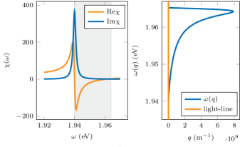
Figure 2: (Left) Real and imaginary parts of the susceptibility according to Eq. (10). We observe a resonance at the exciton energy $\omega_{\text{ex}}=1.94$ eV. The real part of the susceptibility is negative in a small interval from approximately 1.940 eV up to 1.965 eV (shaded region). Only in this spectral region does the monolayer TMD support exciton-polaritons. (Right) Exciton-polariton dispersion relation $\omega_{\mathbf{q}}$ using the approximate expression given in Eq. (13) and the susceptibility presented in the left panel. The spectrum is only finite in the energy window where $\textrm{Re}\chi$ is negative. The polariton’s momentum is much bigger than that of a photon for a given energy, which agrees with the argument used prior to Eq. (13). The parameters of Table 1 were used.

III Lindblad equation

In this section we will determine the Linblad equation for the NV-centers and express the different terms that enter it in terms of exciton-polariton Green’s function.

Tracing out the exciton-polariton degrees of freedom, we obtain the Lindblad equation for the reduced density matrix for the NV-centers in the Schrödinger picture (details of the derivation are provided in Appendix (A)):

$$\dot{\rho}(t) =-\frac{i}{\hbar}\left[\sum_{i}\frac{1}{2}\left(\hbar\omega_{0}+\Delta_{i}\right)\sigma_{i}^{z}+\sum_{i\neq j}g_{ij}\sigma_{i}^{+}\sigma_{j}^{-},\rho(t)\right]$$

$$+\frac{1}{\hbar}\sum_{i,j}\gamma_{ij}\left(\sigma_{j}^{-}\rho(t)\sigma_{i}^{+}-\frac{1}{2}\left\{\sigma_{i}^{+}\sigma_{j}^{-},\rho(t)\right\}\right)$$

$$+\frac{1}{\hbar}\sum_{i,j}\tilde{\gamma}_{ij}\left(\sigma_{j}^{+}\rho(t)\sigma_{i}^{-}-\frac{1}{2}\left\{\sigma_{i}^{-}\sigma_{j}^{+},\rho(t)\right\}\right).$$ (14)

In the above equation $\Delta_{i}$ is the so called Lamb shift, representing the correction to the transition energy of the NV-centers, $g_{ij}$ are couplings between the NV-centers mediated by the exciton-polaritons, $\gamma_{ij}$ and $\tilde{\gamma}_{ij}$ are dissipation coefficients. For a bath in thermal equilibrium and using the quantum fluctuation-dissipation theorem it is possible to express all these quantities in terms of the Green’s functions of the exciton-polaritons. The electric field retarded/advanced Green’s function for exciton-polaritons is defined as

$$D_{\alpha\beta}^{R/A}(t;\mathbf{r}_{i},\mathbf{r}_{j})=\mp\frac{i}{\hbar}\Theta\left(\pm t\right)\left\langle\left[E_{\text{ex-p}}^{\alpha}(t,\mathbf{r}_{i}),E_{\text{ex-p}}^{\beta}(0,\mathbf{r}_{j})\right]\right\rangle_{R}.$$ (15)

where $\left\langle...\right\rangle_{R}$ represents the quantum thermodynamic average over the isolated reservoir degrees of freedom of the bath, and greek indices run over spatial coordinates. Making a Fourier transform in time, $D_{\alpha\beta}^{R/A}(\omega;\mathbf{r}_{i},\mathbf{r}_{j})=\int dte^{i\omega t}D_{\alpha\beta}^{R/A}(t;\mathbf{r}_{i},\mathbf{r}_{j})$, we obtain

$$D_{\alpha\beta}^{R/A}(\omega;\mathbf{r}_{i},\mathbf{r}_{j})=\sum_{\mathbf{q}}\frac{2\omega_{\mathbf{q}}}{\hbar}\frac{E_{\mathbf{q},\text{ex-p}}^{\alpha}(\mathbf{r}_{i})\left(E_{\mathbf{q},\text{ex-p}}^{\beta}(\mathbf{r}_{j})\right)^{*}}{\left(\omega\pm i0^{+}\right)^{2}-\omega_{\mathbf{q}}^{2}}.$$ (16)

The above expression assumes that exciton-polaritons have an infinite lifetime. This is a good approximation at low temperatures, when losses due to coupling of excitons to phonons are very small (Epstein et al., 2020b). Elastic scattering due to impurities is also small (in Sec. V we discuss the role of disorder in more detail). In terms of these Green’s functions, the different coefficients in Eq. (14) are given by

$$\Delta_{i} =\mathcal{P}\int\frac{d\nu}{2\pi}\left[1+2b(\nu)\right]\frac{\mu_{i,\alpha}^{*}A_{\alpha\beta}\left(\nu;\mathbf{r}_{i},\mathbf{r}_{i}\right)\mu_{i,\beta}}{\omega_{0}-\nu},$$ (17)

$$g_{ij} =\mu_{i,\alpha}^{*}D_{\alpha\beta}(\omega_{0};\mathbf{r}_{i},\mathbf{r}_{j})\mu_{j,\beta},$$ (18)

$$\gamma_{ij} =\left[1+b(\omega_{0})\right]\mu_{i,\alpha}^{*}A_{\alpha\beta}\left(\omega_{0};\mathbf{r}_{i},\mathbf{r}_{j}\right)\mu_{j,\beta},$$ (19)

$$\tilde{\gamma}_{ij} =b(\omega_{0})\mu_{j,\alpha}^{*}A_{\alpha\beta}(\omega_{0};\mathbf{r}_{j},\mathbf{r}_{i})\mu_{i,\beta},$$ (20)

where repeated greek indices are summed over, $\mathcal{P}\int$ denotes the Cauchy principal value of the integral, and

$$A_{\alpha\beta}\left(\omega;\mathbf{r}_{i},\mathbf{r}_{j}\right)=i\left[D_{\alpha\beta}^{R}(\omega;\mathbf{r}_{i},\mathbf{r}_{j})-D_{\alpha\beta}^{A}(\omega;\mathbf{r}_{i},\mathbf{r}_{j})\right]$$ (21)

is the electric field exciton-polariton spectral function, and

$$D_{\alpha\beta}(\omega;\mathbf{r}_{i},\mathbf{r}_{j})=\frac{1}{2}\left[D_{\alpha\beta}^{R}(\omega;\mathbf{r}_{i},\mathbf{r}_{j})+D_{\alpha\beta}^{A}(\omega;\mathbf{r}_{i},\mathbf{r}_{j})\right]$$ (22)

is the hermitian part of the Green’s function, which can be written in terms of the spectral function as

$$D_{\alpha\beta}(\omega;\mathbf{r}_{i},\mathbf{r}_{j})=\mathcal{P}\int\frac{d\nu}{2\pi}\frac{A_{\alpha\beta}\left(\nu;\mathbf{r}_{i},\mathbf{r}_{i}\right)}{\omega-\nu}.$$ (23)

For the rest of this work, we will focus on the zero temperature case. In that case one has $\lim_{T\rightarrow 0}b(\nu)=-\Theta(-\nu)$, such that $\lim_{T\rightarrow 0}\left[1+2b(\nu)\right]=\text{sign}(\nu)$ and $b(\omega_{0})=0$, for $\omega_{0}>0$. Therefore, we conclude that in the zero temperature limit $\tilde{\gamma}_{ij}=0$.

We notice that the form of Eqs. (17)-(20) remains valid if we consider coupling of the NV-centers to the all the electromagnetic degrees of freedom, instead of only the polariton mode. In that case, $D_{\alpha\beta}^{R/A}(\omega;\mathbf{r}_{i},\mathbf{r}_{j})$ would be the full electromagnetic Green’s function. For a linear medium, the full electromagnetic Green’s function can be obtained from the classical Maxwell’s equations, as the response function to a point dipole. Replacing the full $D_{\alpha\beta}^{R/A}(\omega;\mathbf{r}_{i},\mathbf{r}_{j})$ by the exciton-polariton contribution amounts to a polariton-pole approximation to the Green’s function, as shown in Appendix (C). This is a good approximation if the exciton-polariton frequency is close to $\omega_{0}$ and if the NV-centers are in close proximity to the TMD.

III.1 Evaluation of the effective couplings and decay rates

Now that we have obtained both the energy window where polaritons may be excited and their dispersion relation we can move on to the explicit calculation of the parameters $\gamma_{ij}$, $\Delta_{i}$ and $g_{ij}$. Starting with $\gamma_{ij}$ and recalling Eqs. (19) and ((16)), we obtain

$$\gamma_{ij}=\frac{2\pi}{\hbar}\sum_{\mathbf{q}}\delta\left(\omega_{0}-\omega_{\mathbf{q}}\right)\bm{\mu}_{i}^{*}\cdot\mathbf{E}_{\mathbf{q},\text{ex-p}}(\mathbf{r}_{i})\mathbf{E}_{\mathbf{q},\text{ex-p}}^{*}(\mathbf{r}_{j})\cdot\bm{\mu}_{j},$$ (24)

Using the previously presented definitions for the mode functions $\mathbf{E}_{\mathbf{q},\text{ex-p}}(\mathbf{r}_{i})$, converting the sum into an integral, performing the angular integration, and finally using the $\delta-$function to compute the remaining integral we find:

$$\gamma_{ij}=\frac{2\pi}{\hbar}\frac{q_{0}}{2\pi}\frac{\hbar\omega_{0}}{2\epsilon_{0}N_{\mathbf{q}_{0}}}\left(\frac{\partial\omega_{\mathbf{q}_{0}}}{\partial q}\right)^{-1}\times\\ \times e^{-\kappa_{1,\mathbf{q}}\left(z_{i}+z_{j}\right)}\mathcal{M}_{ij}(\mathbf{q}_{0},\rho),$$ (25)

where in the reference frame where the dipoles are separated along the $x$ direction:

$$\mathcal{M}_{ij}(\mathbf{q},\rho)=\mu_{i,x}^{*}\mu_{j,x}\left(J_{0}\left(q\rho\right)-\frac{J_{1}\left(q\rho\right)}{q\rho}\right)\\ +\mu_{i,y}^{*}\mu_{j,y}\frac{J_{1}\left(q\rho\right)}{q\rho}+\mu_{i,z}^{*}\mu_{j,z}\frac{q^{2}}{\kappa_{1,\mathbf{q}}^{2}}J_{0}\left(q\rho\right)\\ +\left(\mu_{i,x}^{*}\mu_{j,z}-\mu_{i,z}^{*}\mu_{j,x}\right)\frac{q}{\kappa_{1,\mathbf{q}}}J_{1}(q\rho).$$ (26)

For zero separation, one obtains the simpler form

$$\mathcal{M}_{ij}(\mathbf{q},0) =\frac{1}{2}\left(\mu_{i,x}^{*}\mu_{j,x}+\mu_{i,y}^{*}\mu_{j,y}+\frac{2q^{2}}{\kappa_{1,\mathbf{q}}^{2}}\mu_{i,z}^{*}\mu_{j,z}\right).$$ (27)

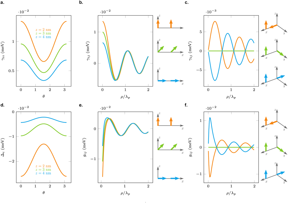
Figure 3: Interaction parameters, energy shifts, and damping constants for different configurations of the system. In panel (a) we depict $\gamma_{11}$ as a function of $\theta$, the angle the dipole makes with the $z$ axis, for three different NV-center–TMD separations. In panel (b) we depict $\gamma_{12}$ as a function of $\rho/\lambda_{p}$, where $\rho$ is the in-plane distance between the NV-centers, and $\lambda_{p}$ is the polariton wavelength for an energy $\hbar\omega_{0}$; in the present case we have $\lambda_{\text{p}}\approx 37$ nm. We consider that both dipoles lie in the x-z plane, with an angle with the z-axis given by $\theta=0,\,\pi/4$ and $\pi/2$ as depicted in the panel. In panel (c) we show $\gamma_{12}$ as a function of $\rho/\lambda_{p}$, for the configurations shown in the panel: with one dipole along the $z$ axis while the other lies in the $x-y$ plane (aligned along $x$, $y$ and $-x$ axes). In panels (d), (e) and (f) show $\Delta_{i}$ and $g_{12}$ for the same dipole orientations as in panels (a), (b) and (c). In all plots, the NV-centers were assumed to be at a distance $z=2$ nm from the TMD. The parameters of Table 1 were used.

To compute the explicit forms of the $\Delta_{i}$ and $g_{ij}$ we can proceed in a similar way to what we have done with the $\gamma_{ij}$, the main difference being that we no longer find closed expressions for these parameters. While for the $\gamma_{ij}$ we had a $\delta-$function that allowed us to compute the integrals in a completely analytical way, for the $\Delta_{i}$ and $g_{ij}$ we will have to compute one of the integrals numerically. Recalling Eqs. (18) and (16), we obtain:

$$g_{ij}=\mathcal{P}\int\frac{dqq}{2\pi}e^{-\kappa_{1,\mathbf{q}}\left(z_{i}+z_{j}\right)}\frac{\omega_{\mathbf{q}}}{2\epsilon_{0}N_{\mathbf{q}}}\times\\ \times\left[\frac{1}{\omega_{0}-\omega_{\mathbf{q}}}-\frac{1}{\omega_{0}+\omega_{\mathbf{q}}}\right]\mathcal{M}_{ij}(\mathbf{q},\rho),$$ (28)

and for the $\Delta_{i}$:

$$\Delta_{i}=\mathcal{P}\int\frac{dqq}{2\pi}e^{-\kappa_{1,\mathbf{q}}\left(z_{i}+z_{j}\right)}\frac{\omega_{\mathbf{q}}}{2\epsilon_{0}N_{\mathbf{q}}}\times\\ \times\left[\frac{1}{\omega_{0}-\omega_{\mathbf{q}}}+\frac{1}{\omega_{0}+\omega_{\mathbf{q}}}\right]\mathcal{M}_{ij}(\mathbf{q},0),$$ (29)

where $\mathcal{M}_{ij}(\mathbf{q},\rho)$ is defined as before

In Fig. 3 we present the plot of $\gamma_{ii}$ as a function of $\theta$ and $\gamma_{ij}$ for different dipole configurations as a function of $\rho$ and $\theta$. In Fig. 3 (a) we depict $\gamma_{ii}$ as a function of the angle the dipole makes with the $z$ axis. We observe that this parameter takes its minimum value when the dipole is parallel to the TMD plane, and the maximum value when it is perpendicular to it. Moreover, we also note the sensitivity of $\gamma_{ii}$ to the dipole–TMD separation. Small increases on this parameter produce significant changes in the final result; as the separation to the TMD plane increases the magnitude of the exciton-polariton induced decay rate diminishes exponentially, in agreement with the analytical expressions previously found. In Fig. 3 (b) we plot $\gamma_{12}$ as a function of $\rho/\lambda_{\text{p}}$, where $\lambda_{p}=2\pi/q(E_{0})\approx 37$ nm, for two parallel dipoles in the $x-z$ plane with different angles with respect to the $z$-axis. We start by noting that, as expected from the different elements of $\mathcal{M}_{ij}$, the parameter $\gamma_{12}$ presents an oscillatory behavior accompanied by a magnitude decrease as $\rho$ increases. Mathematically, this is a consequence of the Bessel functions that appear after the angular integration has been performed leading to a spatial decay proportional to $1/\sqrt{\rho}$ at large distances, where $\rho$ is the distance between NV-centers. Physically, this is a consequence of the two-dimensional nature of the polaritons. Furthermore, we observe that $\gamma_{12}$ is bigger when both dipoles are aligned along the $z$ axis, although the difference between the different orientations becomes negligible for distances greater than one polariton wavelength. Finally, in Fig. 3 (c) we plot $\gamma_{12}$ as a function of $\rho/\lambda_{\text{p}}$, only this time we consider one dipole to be aligned along the $z$ axis, while the other is placed on a plane parallel to the $x-y$ plane with different $\phi$ angles. We first note that, just as in the previous case, $\gamma_{12}$ presents a decaying and oscillatory behavior as $\rho$ increases. Moreover, we note that $\gamma_{12}$ is symmetric when the dipole is aligned along the positive or negative $x$ direction, and it vanishes when it is aligned along the $y$ direction, that is, when the dipole is aligned perpendicularly to the direction connecting the two dipoles.

The plots of $\Delta_{i}$ and $g_{12}$ as a function of $\theta$, the angle the dipole makes with the $z$ axis, and $\rho$ for different dipole configurations are depicted in Figs. 3 (d), (e) and (f). Without surprise, we observe that these quantities present a similar behavior to $\gamma_{ij}$. There are two aspects worthy of consideration. (i) Similarly to $\gamma_{12}$ and for not to small separation, $g_{12}$ decays asymptotically as as $1/\sqrt{\rho}$, being roughly in phase opposition to $\gamma_{12}$. (ii) The magnitude of $\Delta_{i}$ is of the order of 25 $\mu$eV, corresponding to a small energy renormalization of the NV-centers. Comparing the exciton-polariton mediated interaction, $g_{12}$ which decays with $\rho^{-1/2}$, with the electrostatic dipole-dipole interaction, which decays as $\rho^{-3}$, we conclude that the exciton-polariton interaction dominates for $\rho\gtrsim\lambda_{\text{p}}/10$.

IV Exciton mediated superradiance

As noted in Sec. II, our model is a modification of the Dicke Hamiltonian. The modifications are two fold: (i) only a small number (two) of radiant NV-centers are considered; (ii) there is more than one bosonic mode, labeled by the in-plane momentum $\mathbf{q}$. Except for these differences, the model should also present superradiance. The figure of merit allowing to characterize superradiance is Huidobro et al. (2012):

$$\Gamma=\frac{\gamma_{11}+\gamma_{12}+\gamma_{21}+\gamma_{22}}{\gamma_{11}+\gamma_{22}}.$$ (30)

It is known that when $\Gamma>1$ the system shows superradiance (in the opposite regime, the system is subradiant, that is, the emission of coherent radiation is suppressed). In Fig. 4 we depict the figure of merit $\Gamma$. It is clear that depending on the relative position of the two emitters regions exist in space with $\Gamma>1$. This result lays down the basis for discussing the $N-$emitters problem.

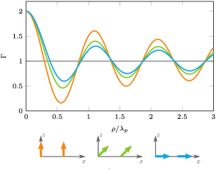
Figure 4: Superradiance and subradiance in the two-coupled NV-centers system. Three orientations of the two electric dipole moments relatively $z-$axis are considered. The parameters are the same as in Fig. 3.

V Conclusions

In this paper we have described the dynamics of two NV-centers, hosted by a diamond, coupled to the exciton-polaritons supported by a monolayer TMD substrate, within the framework of a Lindblad equation. We expressed the exciton-polarion induce dipole-dipole interaction, energy shifts and decay rates of the NV-center two-level systems in terms of a Dyadic Green’s function of the exciton-polariton. We have computed this latter quantity using the modes of the exciton-polaritons alone. We have found that as a consequence of the two dimensional nature of the exciton-polaritons the aforementioned parameters decay in space as $\rho^{-1/2}$. This decay would be stronger with the distance if damping had been considered thus limiting the range of the interaction between two NV-centers. Naturally, the intensity of the exponential decay is tied up to the intensity of the disorder. For small disorder we do not expect an important effect within distances of the order the exciton-polaritons wavelength. An estimation of magnitude of disorder on the calculated parameters can be estimated computing the quantity $f=\exp[-q^{\prime\prime}(\omega)d]$, where $d$ is the distance between the two NV-centers and $q^{\prime\prime}(\omega)$ is the imaginary part of the exciton-polariton wavenumber. For the numbers given in Table 1 and for $d=\lambda_{\text{p}}/2$ we find $f\simeq 0.5$. Therefore, the magnitude of the parameters represented in the figures would be half of what they are for the given $d$.

Our results indicate that TMD exciton-polariton mediated super and subradiance can be observed for NV-centers in diamonds separated by up to 100 nm. These theoretical predictions can be validated experimentally by photoluminescent spectroscopy Scheibner et al. (2007).

Our methods and results are not restricted to NV-centers in diamond, but can be extended to color centers in other materials, such as quantum emitters in hexagonal boron nitride (hBN), which have an electric dipole moment in excess of 2.1 D, that is stronger than for a NV-center in diamond (smaller values of $\mu\sim 0.9-1.1$ D for emitters in hBN have also been reported Noh et al. (2018); Scavuzzo et al. (2019)). Thus, this work opens the door for the study of quantum optics devices fully built with van der Waals heterostructures.

Appendix A Details on the derivation of the Lindblad equation

Here we will provide some details for the derivation of the Linblad equation. To derive the Lindblad equation that governs the NV-center degrees of freedom we will treat the TMD exction-polariton field as a bath which is coupled to the NV-centers via $H_{\text{int}}$ To study the system’s dynamics. The full density matrix of the coupled NV-centers/polaritons, $\chi(t)$, obeys the following equation in the interaction picture (Carmichael, 2002):

$$\dot{\chi}_{I}(t) =-\frac{i}{\hbar}\left[H_{\text{int},I},\chi_{I}(0)\right]$$

$$-\frac{1}{\hbar^{2}}\int_{0}^{t}\left[H_{\text{int},I}(t),\left[H_{\text{int},I}(t^{\prime}),\chi_{I}(t^{\prime})\right]\right]dt^{\prime},$$ (31)

which is easily obtained from the usual equation of motion for density matrices. The derivation of the Lindblad equation for the density of matrix for the NV-centers involves a series of hypothesis and approximations. First, within the Born approximation, it is assumed that at the density matrix can be written as the product of the density matrix of the NV-centers, $\rho(t)$, and the time independent density matrix of the exciton-polariton bath, $R$, i.e. $\chi(t)=\rho(t)\otimes R$. This hypothesis ignores the initial correlation between the two systems and assumes that the perturbation to the bath is small. Next, within the Markov approximation, one replaces $\chi_{I}(t^{\prime})\simeq\rho_{I}(t)\otimes R$ and takes the limit $t\rightarrow\infty$ in the integration in the second term of Eq. (31). These simplification is justified if the characteristic time of the bath is much shorter than the characteristic time of the system, which leads to a loss of memory and Markovian behavior. Finally, within the post-trace rotating wave approximation, only energy conserving terms are kept. Applying these approximations to Eq. (31) and tracing out the degrees of freedom of the exciton-polariton bath, and returning to the Schrödinger picture, the equation of motion for the NV-center density matrix is given by Breuer et al. (2002)

$$\frac{\partial\rho(t)}{\partial t}= -\frac{i}{\hbar}\left[\sum_{i}\frac{1}{2}\hbar\omega_{0}\sigma_{i}^{z}+\sum_{i,j}\sum_{s=\pm}\mu_{i,\alpha}^{s}S_{\alpha\beta}(s\omega_{0};\mathbf{r}_{i},\mathbf{r}_{j})\mu_{j,\beta}^{\bar{s}}\sigma_{i}^{s}\sigma_{j}^{\bar{s}},\rho_{I}(t)\right]$$

$$+\frac{1}{\hbar}\sum_{i,j}\sum_{s=\pm}\mu_{i,\alpha}^{s}\gamma_{\alpha\beta}(s\omega_{0};\mathbf{r}_{i},\mathbf{r}_{j})\mu_{j,\beta}^{\bar{s}}\left(\sigma_{j}^{\bar{s}}\rho_{I}^{S}(t)\sigma_{i}^{s}-\frac{1}{2}\left\{\sigma_{i}^{s}\sigma_{j}^{\bar{s}},\rho_{I}^{S}(t)\right\}\right),$$ (32)

where $\mu_{i,\alpha}^{+}=\mu_{i,\alpha}^{*}$, $\mu_{i,\alpha}^{-}=\mu_{i,\alpha}$, $\bar{s}=-s$, and

$$S_{\alpha\beta}(\omega;\mathbf{r}_{i},\mathbf{r}_{j}) =P\int\frac{d\nu}{2\pi}\left[1+b(\nu)\right]\frac{A_{\alpha\beta}\left(\nu;\mathbf{r}_{i},\mathbf{r}_{j}\right)}{\omega-\nu},$$ (33)

$$\gamma_{\alpha\beta}(\omega;\mathbf{r}_{i},\mathbf{r}_{j}) =\left[1+b(\omega)\right]A_{\alpha\beta}\left(\omega;\mathbf{r}_{i},\mathbf{r}_{j}\right),$$ (34)

with $A_{\alpha\beta}\left(\nu;\mathbf{r}_{i},\mathbf{r}_{j}\right)$ the electric field spectral function. Using the fact that $A_{\alpha\beta}\left(\omega;\mathbf{r}_{i},\mathbf{r}_{j}\right)=-A_{\beta\alpha}\left(-\omega;\mathbf{r}_{j},\mathbf{r}_{i}\right)$, it is easy to see that the dissipators in the main text are given by

$$\gamma_{ij} =\mu_{i,\alpha}^{+}\gamma_{\alpha\beta}(\omega_{0};\mathbf{r}_{i},\mathbf{r}_{j})\mu_{j,\beta}^{-},$$ (35)

$$\tilde{\gamma}_{ij} =\mu_{i,\alpha}^{-}\gamma_{\alpha\beta}(-\omega_{0};\mathbf{r}_{i},\mathbf{r}_{j})\mu_{j,\beta}^{+}.$$ (36)

We will rewrite the terms involving $S_{\alpha\beta}(s\omega_{0};\mathbf{r}_{i},\mathbf{r}_{j})$ by separating the terms with $i\neq j$ and $i=j$. For the term with $i\neq j$, we write

$$\sum_{i\neq j}\sum_{s=\pm}\mu_{i,\alpha}^{s}S_{\alpha\beta}(s\omega_{0};\mathbf{r}_{i},\mathbf{r}_{j})\mu_{j,\beta}^{\bar{s}}\sigma_{i}^{s}\sigma_{j}^{\bar{s}}=\\ =\sum_{i\neq j}\mu_{i,\alpha}^{+}S_{\alpha\beta}(\omega_{0};\mathbf{r}_{i},\mathbf{r}_{j})\mu_{j,\beta}^{-}\sigma_{i}^{+}\sigma_{j}^{-}+\mu_{i,\alpha}^{-}S_{\alpha\beta}(-\omega_{0};\mathbf{r}_{i},\mathbf{r}_{j})\mu_{j,\beta}^{+}\sigma_{i}^{-}\sigma_{j}^{+}\\ =\sum_{i\neq j}\mu_{i,\alpha}^{+}S_{\alpha\beta}(\omega_{0};\mathbf{r}_{i},\mathbf{r}_{j})\mu_{j,\beta}^{-}\sigma_{i}^{+}\sigma_{j}^{-}+\mu_{j,\beta}^{-}S_{\beta\alpha}(-\omega_{0};\mathbf{r}_{j},\mathbf{r}_{i})\mu_{i,\alpha}^{+}\sigma_{j}^{-}\sigma_{i}^{+}.$$ (37)

Using the fact that $\left[\sigma_{i}^{+},\sigma_{j}^{-}\right]=0$ for $i\neq j$, we can write

$$\sum_{i\neq j}\sum_{s=\pm}\mu_{i,\alpha}^{s}S_{\alpha\beta}(s\omega_{0};\mathbf{r}_{i},\mathbf{r}_{j})\mu_{j,\beta}^{\bar{s}}\sigma_{i}^{s}\sigma_{j}^{\bar{s}}=\sum_{i\neq j}g_{ij}\sigma_{i}^{+}\sigma_{j}^{-}.$$ (38)

where

$$g_{ij} =\mu_{i,\alpha}^{+}\left[S_{\alpha\beta}(\omega_{0};\mathbf{r}_{i},\mathbf{r}_{j})+S_{\beta\alpha}(-\omega_{0};\mathbf{r}_{j},\mathbf{r}_{i})\right]\mu_{j,\beta}^{-}$$

$$=P\int\frac{d\nu}{2\pi}\frac{\mu_{i,\alpha}^{+}A_{\alpha\beta}\left(\nu;\mathbf{r}_{i},\mathbf{r}_{j}\right)\mu_{j,\beta}^{-}}{\omega_{0}-\nu}$$

$$=\mu_{i,\alpha}^{+}D_{\alpha\beta}\left(\omega_{0};\mathbf{r}_{i},\mathbf{r}_{j}\right)\mu_{j,\beta}^{-}.$$ (39)

For the term with $i=j$ we write

$$\sum_{i}\sum_{s=\pm}\mu_{i,\alpha}^{s}S_{\alpha\beta}(s\omega_{0};\mathbf{r}_{i},\mathbf{r}_{i})\mu_{j,\beta}^{\bar{s}}\sigma_{i}^{s}\sigma_{i}^{\bar{s}}=\sum_{i}\mu_{i,\alpha}^{+}S_{\alpha\beta}(\omega_{0};\mathbf{r}_{i},\mathbf{r}_{i})\mu_{i,\beta}^{-}\sigma_{i}^{+}\sigma_{i}^{-}+\mu_{i,\alpha}^{-}S_{\alpha\beta}(-\omega_{0};\mathbf{r}_{i},\mathbf{r}_{i})\mu_{i,\beta}^{+}\sigma_{i}^{-}\sigma_{i}^{+}.$$ (40)

Noticing that

$$\sigma_{i}^{+}\sigma_{i}^{-} =\left|e,i\right\rangle\left\langle e,i\right|$$ (41)

$$\sigma_{i}^{-}\sigma_{i}^{+} =\left|g,i\right\rangle\left\langle g,i\right|$$ (42)

We can then write

$$\sum_{i}\sum_{s=\pm}\mu_{i,\alpha}^{s}S_{\alpha\beta}(s\omega_{0};\mathbf{r}_{i},\mathbf{r}_{i})\mu_{j,\beta}^{\bar{s}}\sigma_{i}^{s}\sigma_{i}^{\bar{s}}=\frac{1}{2}\tilde{\Delta}_{i}\sigma_{i}^{0}+\frac{1}{2}\Delta_{i}\sigma_{i}^{z},$$ (43)

where $\sigma_{i}^{0}=\left|e,i\right\rangle\left\langle e,i\right|+\left|g,i\right\rangle\left\langle g,i\right|$,

$$\Delta_{i} =\mu_{i,\alpha}^{+}\left[S_{\alpha\beta}(\omega_{0};\mathbf{r}_{i},\mathbf{r}_{i})-S_{\beta\alpha}(-\omega_{0};\mathbf{r}_{i},\mathbf{r}_{i})\right]\mu_{i,\beta}^{-}$$

$$=P\int\frac{d\nu}{2\pi}\left[1+2b(\nu)\right]\frac{\mu_{i,\alpha}^{+}A_{\alpha\beta}\left(\nu;\mathbf{r}_{i},\mathbf{r}_{i}\right)\mu_{i,\beta}^{-}}{\omega_{0}-\nu},$$ (44)

and

$$\tilde{\Delta}_{i} =\mu_{i,\alpha}^{+}\left[S_{\alpha\beta}(\omega_{0};\mathbf{r}_{i},\mathbf{r}_{i})+S_{\beta\alpha}(-\omega_{0};\mathbf{r}_{i},\mathbf{r}_{i})\right]\mu_{i,\beta}^{-}$$

$$=P\int\frac{d\nu}{2\pi}\frac{\mu_{i,\alpha}^{+}A_{\alpha\beta}\left(\nu;\mathbf{r}_{i},\mathbf{r}_{i}\right)\mu_{i,\beta}^{-}}{\omega_{0}-\nu}$$

$$=\mu_{i,\alpha}^{+}D_{\alpha\beta}\left(\omega_{0};\mathbf{r}_{i},\mathbf{r}_{i}\right)\mu_{i,\beta}^{-}.$$ (45)

If the NV-centers are equal, we have $\tilde{\Delta}_{1}=\tilde{\Delta}_{2}$, and therefore, this term only leads to a global shift in energy, which can therefore be ignored.

Appendix B Mode length and Green’s function

In this appendix we give further insight on the derivation of the mode length and Green function presented in the main text.

Following Ref. Ferreira et al. (2020), the mode length is defined as:

$$N(\mathbf{q})=\int\mathbf{A}_{\mathbf{q}}^{*}(z)\cdot\left(\bar{\epsilon}_{r}(z)+\frac{\omega}{2}\frac{\partial}{\partial\omega}\bar{\epsilon}_{r}(z)\right)\cdot\mathbf{A}_{\mathbf{q}}(z)dz,$$ (46)

where:

$$\epsilon_{r}(z)=\bar{\epsilon}_{d}(z)+\frac{i\bar{\sigma}(\omega)}{\epsilon_{0}\omega}\delta(z),$$ (47)

with $\bar{\epsilon}_{d}(z)$ the dielectric function tensor of the different layers composing the system, $\bar{\sigma}(\omega)$ the conductivity tensor of the TMD and:

$$\mathbf{A}_{\mathbf{q}}(z)=\begin{cases}\mathbf{u}_{1,\mathbf{q}}^{+}e^{-\kappa_{1,\mathbf{q}}z}&z>0\\ \mathbf{u}_{2,\mathbf{q}}^{-}e^{\kappa_{2,\mathbf{q}}z}&z<0\end{cases}$$

where:

$$\mathbf{u}_{n,\mathbf{q}}^{\pm}=i\frac{\mathbf{q}}{q}\mp\frac{q}{\kappa_{n,\mathbf{q}}}\hat{\mathbf{z}}.$$ (48)

Noting that the conductivity tensor only couples to the in-plane degrees of freedom, and observing that the exciton conductivity can be written as:

$$\frac{\sigma(\omega)}{\epsilon_{0}\omega}=-id\chi_{bg}+i\frac{df_{\text{ex}}}{2}\frac{\omega_{\text{ex}}^{2}}{\omega^{2}-\omega_{ex}^{2}},$$ (49)

where the imaginary part of the susceptibility $\chi(\omega)$ was discarded, we find:

$$N(\mathbf{q})=\frac{\epsilon_{1}}{2}\frac{\kappa_{1,\mathbf{q}}^{2}+q^{2}}{\kappa_{1,\mathbf{q}}^{3}}+\frac{\epsilon_{2}}{2}\frac{\kappa_{2,\mathbf{q}}^{2}+q^{2}}{\kappa_{2,\mathbf{q}}^{3}}+\frac{i\sigma(\omega)}{2\epsilon_{0}\omega}+\frac{i}{2\epsilon_{0}}\frac{\partial\sigma(\omega)}{\partial\omega}\\ =\frac{\epsilon_{1}}{2}\frac{\kappa_{1,\mathbf{q}}^{2}+q^{2}}{\kappa_{1,\mathbf{q}}^{3}}+\frac{\epsilon_{2}}{2}\frac{\kappa_{2,\mathbf{q}}^{2}+q^{2}}{\kappa_{2,\mathbf{q}}^{3}}+\\ +\frac{1}{2}df_{\text{ex}}\frac{\omega_{\text{ex}}^{4}}{\left(\omega_{\mathbf{q}}^{2}-\omega_{\text{ex}}^{2}\right)^{2}}+d\chi_{bg}.$$ (50)

The vector potential operator for the exciton-polariton is therefore, written as

$$\mathbf{A}_{\text{ex-p}}(\mathbf{r})=\sum_{\mathbf{q}}\left(\mathbf{A}_{\mathbf{q},\text{ex-p}}(\mathbf{r})a_{\mathbf{q}}+\mathbf{A}_{\mathbf{q},\text{ex-p}}^{*}(\mathbf{r})a_{\mathbf{q}}^{\dagger}\right)$$ (51)

where

$$\mathbf{A}_{\mathbf{q},\text{ex-p}}(\mathbf{r})=\sqrt{\frac{\hbar}{2A\epsilon_{0}\omega_{\mathbf{q}}N(\mathbf{q})}}\times\\ \times e^{-\kappa_{1,\mathbf{q}}z}e^{i\mathbf{q}\cdot\mathbf{x}}\begin{cases}\left(i\frac{\mathbf{q}}{q}-\frac{q}{\kappa_{1,\mathbf{q}}}\hat{\mathbf{z}}\right)e^{-\kappa_{1,\mathbf{q}}z},&z>0\\ \left(i\frac{\mathbf{q}}{q}+\frac{q}{\kappa_{2,\mathbf{q}}}\hat{\mathbf{z}}\right)e^{\kappa_{2,\mathbf{q}}z},&z<0\end{cases}$$ (52)

The electric field operator for the exciton-polariton is then given by Eq. (6), with $\mathbf{E}_{\mathbf{q},\text{ex-p}}(\mathbf{r})=i\omega_{\mathbf{q}}\mathbf{A}_{\mathbf{q},\text{ex-p}}(\mathbf{r})$.

Appendix C Exciton-polariton Green’s function as a polariton-pole approximation

In this appendix we will show how the exciton-polariton Green’s function emerges as a polariton-pole approximation to the full electric field Green’s function. For the structure considered in this work, the Green’s function can be written as (for $z_{i},z_{j}>0$):

$$\bm{D}^{R}(\omega;\mathbf{r}_{i},\mathbf{r}_{j})=\bm{D}^{R,0}(\omega;\mathbf{r}_{i},\mathbf{r}_{j})\\ +\frac{1}{A}\sum_{\mathbf{q},\lambda}e^{i\mathbf{q}\cdot\left(\mathbf{x}_{i}-\mathbf{x}_{j}\right)}\bm{D}_{\lambda}^{R}(\omega;\mathbf{q},z_{i},z_{j}),$$ (53)

where $\bm{D}^{R,0}(\omega;\mathbf{r}_{i},\mathbf{r}_{j})$ is the Green’s function for the field in vacuum and $\bm{D}_{\lambda}^{R}(\omega;\mathbf{q},z_{i},z_{j})$ is the reflected Green’s function for the $\lambda=s,p$ polarization. These are given by

$$\bm{D}_{\lambda}^{R}(\omega;\mathbf{q}_{i},z_{i},z_{j})=-\mu_{0}\omega^{2}\frac{i}{2k_{z,1}}r_{\lambda}e^{ik_{z,1}\left(z_{i}+z_{j}\right)}\mathbf{e}_{\lambda,1}^{+}\otimes\mathbf{e}_{\lambda,1}^{-},$$ (54)

where $k_{z,n}=i\kappa_{n}$, $\mathbf{e}_{\lambda,n}^{\pm}$ are polarization vectors and $r_{\lambda}$ reflection coefficients for the $\lambda=s,p$ polarizations. Focusing on the $p$-polarization, we have

$$\mathbf{e}_{p,n}^{\pm} =\frac{q}{k_{n}}\mathbf{e}_{z}\mp\frac{k_{z,n}}{k_{n}}\frac{\mathbf{q}}{q},$$ (55)

$$r_{p} =\frac{\frac{\omega^{2}\epsilon_{2}}{\kappa_{2}}-\frac{\omega^{2}\epsilon_{1}}{\kappa_{1}}+\frac{i}{\epsilon_{0}}\omega\sigma(\omega)}{\frac{\omega^{2}\epsilon_{2}}{\kappa_{2}}+\frac{\omega^{2}\epsilon_{1}}{\kappa_{1}}+\frac{i}{\epsilon_{0}}\omega\sigma(\omega)}$$ (56)

with $k_{n}^{2}=\epsilon_{1}\omega^{2}/c^{2}$. At the exciton-polariton dispersion relation, $r_{p}$ has a pole. Let us expand the Green’s function around this pole. Defining

$$d_{\mathbf{q}}(\omega)=\frac{\omega^{2}\epsilon_{2}}{\kappa_{z,2}}+\frac{\omega^{2}\epsilon_{1}}{\kappa_{z,1}}+\frac{i}{\epsilon_{0}}\omega\sigma(\omega),$$ (57)

the exciton-polariton dispersion relation is defined by $d_{\mathbf{q}}(\omega_{\mathbf{q}})=0$. Expanding $d_{\mathbf{q}}(\omega)$ around $\omega_{\mathbf{q}}$ and keeping only the imaginary part of $\sigma(\omega)$, we obtain

$$d_{\mathbf{q}}(\omega)\simeq\left.\frac{\partial d_{\mathbf{q}}(\omega)}{\partial\left(\omega^{2}\right)}\right|_{\omega=\omega_{\mathbf{q}}}\left(\omega^{2}-\omega_{\mathbf{q}}^{2}\right),$$ (58)

where

$$\left.\frac{\partial d_{\mathbf{q}}(\omega)}{\partial\left(\omega^{2}\right)}\right|_{\omega=\omega_{\mathbf{q}}}=\left.\frac{\epsilon_{1}\left(q^{2}+\kappa_{z,1}^{2}\right)}{2\kappa_{z,1}^{3}}\right|_{\omega=\omega_{\mathbf{q}}}+\\ \left.\frac{\epsilon_{2}\left(q^{2}+\kappa_{z,2}^{2}\right)}{2\kappa_{z,2}^{3}}\right|_{\omega=\omega_{\mathbf{q}}}+\frac{i}{\epsilon_{0}}\left.\frac{\partial\left(\omega\sigma(\omega)\right)}{\partial\left(\omega^{2}\right)}\right|_{\omega=\omega_{\mathbf{q}}},$$ (59)

which we recognize to be nothing, but the mode length, $N_{\mathbf{q}}$. Therefore, we obtain the polariton-pole contribution to reflection coefficient

$$r_{p}\simeq\left[-\frac{2\omega_{\mathbf{q}}^{2}\epsilon_{1}}{\kappa_{z,1}}\right]_{\omega=\omega_{p}}\frac{1}{N_{\mathbf{q}}}\frac{1}{\omega^{2}-\omega_{\mathbf{q}}^{2}}$$ (60)

approximating the full Green’s function by its polariton-pole contribution, we obtain

$$\bm{D}^{R}(\omega;\mathbf{r}_{i},\mathbf{r}_{j})\simeq\frac{1}{A}\sum_{\mathbf{q},\lambda}e^{i\mathbf{q}\cdot\left(\mathbf{x}_{i}-\mathbf{x}_{j}\right)}e^{-\kappa_{1}\left(z_{i}+z_{j}\right)}\frac{2\omega_{\mathbf{q}}}{\omega^{2}-\omega_{\mathbf{q}}^{2}}\\ \frac{\omega_{\mathbf{q}}}{2\epsilon_{0}N_{\mathbf{q}}}\left[i\frac{\mathbf{q}}{q}-\frac{q}{\kappa_{1,\mathbf{q}}}\mathbf{e}_{z}\right]\otimes\left[-i\frac{\mathbf{q}}{q}-\frac{q}{\kappa_{1,\mathbf{q}}}\mathbf{e}_{z}\right],$$ (61)

which coincides with Eq. 16 of the main text.

References

- Jelezko and Wrachtrup (2006) F. Jelezko and J. Wrachtrup, physica status solidi (a) 203, 3207 (2006).
- Hong et al. (2013) S. Hong, M. S. Grinolds, L. M. Pham, D. Le Sage, L. Luan, R. L. Walsworth, and A. Yacoby, MRS Bulletin 38, 155 (2013).
- Doherty et al. (2013) M. W. Doherty, N. B. Manson, P. Delaney, F. Jelezko, J. Wrachtrup, and L. C. L. Hollenberg, Physics Reports 528, 1 (2013).
- Ohashi et al. (2013) K. Ohashi, T. Rosskopf, H. Watanabe, M. Loretz, Y. Tao, R. Hauert, S. Tomizawa, T. Ishikawa, J. Ishi-Hayase, S. Shikata, C. L. Degen, and K. M. Itoh, Nano Lett. 13, 4733 (2013).
- Hauf et al. (2011) M. V. Hauf, B. Grotz, B. Naydenov, M. Dankerl, S. Pezzagna, J. Meijer, F. Jelezko, J. Wrachtrup, M. Stutzmann, F. Reinhard, and J. A. Garrido, Phy. Rev. B 83, 081304 (2011).
- Fu et al. (2010) K. M. C. Fu, C. Santori, P. E. Barclay, and R. G. Beausoleil, Appl. Phys. Lett. 96, 121907 (2010).
- Doherty et al. (2011) M. W. Doherty, N. B. Manson, P. Delaney, and L. C. L. Hollenberg, New J. Phys. 13, 025019 (2011).
- Lillie et al. (2019) S. E. Lillie, N. Dontschuk, D. A. Broadway, D. L. Creedon, L. C. L. Hollenberg, and J.-P. Tetienne, Phys. Rev. Applied 12, 024018 (2019).
- Chu and Lukin (2017) Y. Chu and M. D. Lukin, “Quantum optics and nanophotonics,” (OUP, 2017) Chap. Quantum optics with nitrogen-vacancy centres in diamond.
- Liu et al. (2013) S. Liu, R. Yu, J. Li, and Y. Wu, J. Appl. Phys. 114, 244306 (2013).
- Thiering et al. (2020) G. Thiering, A. Gali, C. E. Nebel, I. Aharonovich, N. Mizuochi, and M. Hatano, “Chapter one - color centers in diamond for quantum applications,” in Semiconductors and Semimetals, Vol. 103 (Elsevier, 2020) pp. 1–36.
- Schirhagl et al. (2014) R. Schirhagl, K. Chang, M. Loretz, and C. L. Degen, Annu. Rev. Phys. Chem. 65, 83 (2014).
- Bernien et al. (2013) H. Bernien, B. Hensen, W. Pfaff, G. Koolstra, M. S. Blok, L. Robledo, T. H. Taminiau, M. Markham, D. J. Twitchen, L. Childress, and R. Hanson, Nature 497, 86 (2013).
- Sipahigil et al. (2014) A. Sipahigil, K. D. Jahnke, L. J. Rogers, T. Teraji, J. Isoya, A. S. Zibrov, F. Jelezko, and M. D. Lukin, Phys. Rev. Lett. 113, 113602 (2014).
- Bradac et al. (2019) C. Bradac, W. Gao, J. Forneris, M. E. Trusheim, and I. Aharonovich, Nature Comm. 10, 5625 (2019).
- Acosta et al. (2019) V. M. Acosta, L. S. Bouchard, D. Budker, R. Folman, T. Lenz, P. Maletinsky, D. Rohner, Y. Schlussel, and L. Thiel, Journal of Superconductivity and Novel Magnetism 32, 85 (2019).
- Dolde et al. (2014) F. Dolde, M. W. Doherty, J. Michl, I. Jakobi, B. Naydenov, S. Pezzagna, J. Meijer, P. Neumann, F. Jelezko, N. B. Manson, and J. Wrachtrup, Phys. Rev. Lett. 112, 097603 (2014).
- Lehmberg (1970) R. H. Lehmberg, Phys. Rev. A 2, 883 (1970).
- Gonzalez-Tudela et al. (2011) A. Gonzalez-Tudela, D. Martin-Cano, E. Moreno, L. Martin-Moreno, C. Tejedor, and F. J. Garcia-Vidal, Phys. Rev. Lett. 106, 020501 (2011).
- Martín-Cano et al. (2011) D. Martín-Cano, A. González-Tudela, L. Martín-Moreno, F. J. García-Vidal, C. Tejedor, and E. Moreno, Phys. Rev. B 84, 235306 (2011).
- Zhou et al. (2017) L.-M. Zhou, P.-J. Yao, N. Zhao, and F.-W. Sun, J. Phys. B: Atom., Mol. and Opt. Phys. 50, 165501 (2017).
- Törmä and Barnes (2014) P. Törmä and W. L. Barnes, Rep. Prog. Phys. 78, 013901 (2014).
- Delga et al. (2014) A. Delga, J. Feist, J. Bravo-Abad, and F. J. Garcia-Vidal, J. of Opt. 16, 114018 (2014).
- Huidobro et al. (2012) P. A. Huidobro, A. Y. Nikitin, C. González-Ballestero, L. Martín-Moreno, and F. J. García-Vidal, Phys. Rev. B 85, 155438 (2012).
- Chaudhary et al. (2019) K. Chaudhary, M. Tamagnone, M. Rezaee, D. K. Bediako, A. Ambrosio, P. Kim, and F. Capasso, Sci. Adv. 5, eaau7171 (2019).
- Chen and Chen (2007) D.-Z. A. Chen and G. Chen, Appl. Phys. Lett. 91, 121906 (2007).
- Epstein et al. (2020a) I. Epstein, A. Chaves, D. A. Rhodes, B. Frank, K. Watanabe, T. Taniguchi, H. Giessen, J. C. Hone, N. M. R. Peres, and F. H. L. Koppens, 2D Materials 7, 035031 (2020a).
- Quinteiro et al. (2006) G. F. Quinteiro, J. Fernández-Rossier, and C. Piermarocchi, Phys. Rev. Lett. 97, 097401 (2006).
- BrasilI et al. (2013) C. A. BrasilI, F. F. FanchiniII, and R. de Jesus Napolitano III, Rev. Bras. Ensino Fís. 35, 1303 (2013).
- Schaller (2014) G. Schaller, Open Quantum Systems Far from Equilibrium, 1st ed., Lecture Notes in Physics (Springer, Heidelberg, 2014).
- Garraway (2011) B. M. Garraway, Philosophical Transactions of the Royal Society A: Mathematical, Physical and Engineering Sciences 369, 1137 (2011).
- Cong et al. (2016) K. Cong, Q. Zhang, Y. Wang, G. T. Noe, A. Belyanin, and J. Kono, J. Opt. Soc. Am. B 33, C80 (2016).
- Kirton et al. (2019) P. Kirton, M. M. Roses, J. Keeling, and E. G. Dalla Torre, Adv. Quantum Technol. 2, 1800043 (2019).
- Cortes et al. (2020) C. L. Cortes, M. Otten, and S. K. Gray, J. Chem. Phys. 152, 084105 (2020).
- Tamarat et al. (2006) P. Tamarat, T. Gaebel, J. R. Rabeau, M. Khan, A. D. Greentree, H. Wilson, L. C. L. Hollenberg, S. Prawer, P. Hemmer, F. Jelezko, and J. Wrachtrup, Phys. Rev. Lett. 97, 083002 (2006).
- (36) As a reference, the dipole moment of the first excited state of the Hydrogen atom is D.
- Gali (2019) Á. Gali, Nanophotonics 8, 1907 (2019).
- Ferreira et al. (2020) B. A. Ferreira, B. Amorim, A. J. Chaves, and N. M. R. Peres, Phys. Rev. A 101, 033817 (2020).
- You et al. (2020) C. You, A. C. Nellikka, I. D. Leon, and O. S. Magaña-Loaiza, Nanophotonics 9, 1243 (2020).
- Moradi (2020) A. Moradi, Canonical Problems in the Theory of Plasmonics: From 3D to 2D Systems, 1st ed., Springer Series in Optical Sciences (Springer, Berlim, 2020).
- Wang et al. (2018) G. Wang, A. Chernikov, M. M. Glazov, T. F. Heinz, X. Marie, T. Amand, and B. Urbaszek, Rev. Mod. Phys. 90, 021001 (2018).
- Molina-Sánchez and Wirtz (2011) A. Molina-Sánchez and L. Wirtz, Phys. Rev. B 84, 155413 (2011).
- Gonçalves and Peres (2015) P. A. D. Gonçalves and N. M. R. Peres, An Introduction to Graphene Plasmonics (World Scientific, Singapore, 2015).
- Ferreira et al. (2019) F. Ferreira, A. J. Chaves, N. M. R. Peres, and R. M. Ribeiro, J. Opt. Soc. Am. B 36, 674 (2019).
- Epstein et al. (2020b) I. Epstein, B. Terrés, A. Chaves, V.-V. Pusapati, D. A. Rhodes, B. Frank, V. Zimmermann, Y. Qin, K. Watanabe, T. Taniguchi, H. Giessen, S. Tongay, J. C. Hone, N. M. R. Peres, and F. H. L. Koppens, Nano Lett. 20, 3545 (2020b).
- Scheibner et al. (2007) M. Scheibner, T. Schmidt, L. Worschech, A. Forchel, G. Bacher, T. Passow, and D. Hommel, Nat. Phys. 3, 106 (2007).
- Noh et al. (2018) G. Noh, D. Choi, J.-H. Kim, D.-G. Im, Y.-H. Kim, H. Seo, and J. Lee, Nano Lett. 18, 4710 (2018).
- Scavuzzo et al. (2019) A. Scavuzzo, S. Mangel, J.-H. Park, S. Lee, D. Loc Duong, C. Strelow, A. Mews, M. Burghard, and K. Kern, Appl. Phys. Lett. 114, 062104 (2019).
- Carmichael (2002) H. J. Carmichael, Statistical Methods in Quantum Optics 1, 2nd ed., Texts and Monographs in Physics, Vol. 1 (Springer, Berlim, 2002).
- Breuer et al. (2002) H.-P. Breuer, F. Petruccione, et al., The theory of open quantum systems (Oxford University Press, 2002).