Fast computation of hyperelliptic curve isogenies in odd characteristic

Abstract.

Let $p$ be an odd prime number and $g\geq 2$ be an integer. We present an algorithm for computing explicit rational representations of isogenies between Jacobians of hyperelliptic curves of genus $g$ over an extension $K$ of the field of $p$-adic numbers $\mathbb{Q}_{p}$. It relies on an efficient resolution, with a logarithmic loss of $p$-adic precision, of a first order system of differential equations.

1. Introduction

After exploring elliptic curves in cryptography and their isogenies, and interest has been raised to their generalizations. Researchers began to inspect principally polarized abelian varieties, especially Jacobians of genus two and three curves and compute isogenies between them [CR15, CE15, Mil19, Tia20]. Their main interest was to calculate the number of points of these varieties over finite fields [GS12, LL06, BGG⁺17] and more recently to instantiate isogeny-based cryptography schemes [FT19, CS20]. In this work, we concentrate on the problem of computing explicitly isogenies between Jacobians of hyperelliptic curves over finite fields of odd characteristic, this will be a generalization to [CE15] and [Mil19].
A separable isogeny between Jacobians of hyperelliptic curves of genus $g$ defined over a field $k$ is characterized by its so called rational representation $($see Section 2.2 for the definition$)$; it is a compact writing of the isogeny and can be expressed by $2g$ rational fractions defined over a finite extension of $k$. These rational fractions are related. In fields of characteristic different from $2$, they can be determined by computing an approximation of the solution $X(t)\in k\llbracket t\rrbracket{}^{g}$ of a first order non-linear system of differential equations of the form

$$H\left(X(t)\right)\cdot X^{\prime}(t)=G(t)$$ (1)

where $H\!:k\llbracket t\rrbracket{}^{g}\rightarrow{M}_{g}\!\left(k\llbracket t\rrbracket\right)$ is a well chosen map and $G(t)\!\in\!k\llbracket t\rrbracket{}^{g}$. This approach is a generalization of the elliptic curves case [LV16] for which Equation (1) is solved in dimension one.
Equation (1) was first introduced in [CE15] for genus two curves defined over finite fields of odd characteristic and solved in [KPR20] using a well-designed algorithm based on a Newton iteration; this allowed them to compute $X(t)$ modulo $t^{O({\ell})}$ in the case of an $(\ell,\ell)$-isogeny for a cost of $\tilde{O}(\ell)$ operations in $k$ then recover the rational fractions that defines the rational representation of the isogeny. This approach does not work when the characteristic of $k$ is positive and small compared to $\ell$, in which case divisions by $p$ occur and an error can be raised while doing the computations. We take on this issue similarly as in the elliptic curve case ([LS08, CEL20]) by lifting the problem to the $p$-adics. We will always suppose that the lifted Jacobians are also Jacobians for some hyperelliptic curves. It is relevant to assume this, even though it is not the generic case when $g$ is greater than $3$ [OS86], since it allows us to compute efficiently the rational representation of the multiplication by an integer which in this case the lifting can be done arbitrarily. After this process, we need to analyze the loss of $p$-adic precision in order to solve Equation (1) without having a numerical instability. We extend the result of [LV16], by proving that the number of lost digits when computing an approximation of the solution of Equation (1) modulo $t^{O(g\ell)}$, stays within $O\left(\log_{p}(g\ell)\right)$. Our main theorem is the following.

Theorem.

Let $p$ be a prime number. Let $K$ be a finite extension of $\mathbb{Q}_{p}$ and $\mathcal{O}_{K}$ be its ring of integers. There exists an algorithm that takes as input:

• three positive integers $n$,$g$ and $N$,

• a map $H\!:\mathcal{O}_{K}\llbracket t\rrbracket{}^{g}\rightarrow M_{g}\!\left(\mathcal{O}_{K}\llbracket t\rrbracket\right)$ such that $H(0)\in\text{GL}_{g}\left(\mathcal{O}_{K}\right)$,

• a vector $G(t)\in\mathcal{O}_{K}\llbracket t\rrbracket{}^{g}$,

and, assuming that the differential equation

$$H\left(X(t)\right)\cdot X^{\prime}(t)=G(t)$$

admits a unique solution in $\left(t\mathcal{O}_{K}\llbracket t\rrbracket\right)^{g}$, outputs an approximation of this solution modulo $(p^{N},t^{n+1})$ for a cost $\tilde{O}\left(g^{\omega}n\right)$, where $\omega\in[2,3[$ is the exponent of matrix multiplication, at precision $O(p^{M})$ with $M=\max(N,3)+\lfloor\log_{p}(n)\rfloor$ if $p=2$, $M=\max(N,2)+\lfloor\log_{p}(n)\rfloor$ if $p=3$ and $M=N+\lfloor\log_{p}(n)\rfloor$ otherwise.

One can do a bit better for $p=2$ and $3$ if we follow the same strategy as [LV16], in this case $M$ is equal to $\max(N,2)+\lfloor\log_{p}(n)\rfloor$ if $p=2$ and $N+\lfloor\log_{p}(n)\rfloor$ otherwise. For the sake of simplicity, we will not prove this here.

Note that this technique does not allow to compute isogenies in characteristic two for several reasons. First, the general equation of a hyperelliptic curve in characteristic two does not have the same form as in odd characteristic. Moreover, the map $H$ includes square roots of polynomials which implies that solving Equation (1) will require to extract square roots at some point. However, it is well known that extracting square roots in an extension of $\mathbb{Q}_{2}$ is an unstable operation. Still, it is quite interesting to solve Equation (1) for $p=2$ with the assumptions that we made in the main theorem, even thought this approach does not lead to the computation of isogenies between Jacobians of hyperelliptic curves.

2. Jacobians of curves and their isogenies

Throughout this section, the letter $k$ refers to a fixed field of characteristic different from two. Let $\bar{k}$ be a fixed algebraic closure of $k$. In Section 2.1, we briefly recall some basic elements about principally polarized abelian varieties and $(\ell,\ldots,\ell)$-isogenies between them; the notion of rational representation is discussed in Section 2.2. Finally, for a given rational representation, we construct a system of differential equations that we associate with it.

2.1. $(\ell,\cdots,\ell)$-isogenies between abelian varieties

Let $A$ be an abelian variety of dimension $g$ over $k$ and $A^{\vee}$ be its dual. To a fixed line bundle $\mathcal{L}$ on $A$, we associate the morphism $\lambda_{\mathcal{L}}$ defined as follows

$$\begin{array}[]{rcl}\lambda_{\mathcal{L}}\,:\>A&\longrightarrow&A^{\vee}\\ x&\longmapsto&t_{x}^{*}\mathcal{L}\otimes\mathcal{L}^{-1}\end{array}$$

where $t_{x}$ denotes the translation by $x$ and $t_{x}^{*}\mathcal{L}$ is the pullback of $\mathcal{L}$ by $t_{x}$.
We recall from [Mil86] that a polarization $\lambda$ of $A$ is an isogeny $\lambda:\,A\longrightarrow A^{\vee}$, that is a surjective homomorphism of abelian varieties of finite kernel, such that over $\bar{k}$, $\lambda$ is of the form $\lambda_{\mathcal{L}}$ for some ample line bundle $\mathcal{L}$ on $A_{\bar{k}}:=A\otimes\text{Spec}(\bar{k})$. When the degree of a polarization $\lambda$ of $A$ is equal to $1$, we say that $\lambda$ is a principal polarization and the pair $(A,\lambda)$ is a principally polarized abelian variety. We assume in the rest of this subsection that we are given a principally polarized abelian variety $(A,\lambda)$. The Rosati involution on the ring End$(A)$ of endomorphsims of $A$ corresponding to the polarization $\lambda$ is the map

$$\begin{array}[]{rcl}\text{ End}(A)&\longrightarrow&\text{End}(A)\\ \alpha&\longmapsto&\lambda^{-1}\circ\alpha^{\vee}\circ\lambda.\end{array}$$

The Rosati involution is crucial for the study of the division algebra End$(A)\otimes\mathbb{Q}$, but for our purpose, we only state the following result.

Proposition 1.

[Mil86, Proposition 14.2] For every $\alpha\in$ End$\,\!(A)$ fixed by the Rosati involution, there exists, up to algebraic equivalence, a unique line bundle $\mathcal{L}_{A}^{\alpha}$ on $A$ such that $\lambda_{\mathcal{L}_{A}^{\alpha}}=\lambda\circ\alpha$.

In particular, taking $\alpha$ to be the identity endomorphism denoted “$1$”, there exists a unique line bundle $\mathcal{L}_{A}^{1}$ such that $\lambda_{\mathcal{L}_{A}^{1}}=\lambda$.
Using Proposition 1, we give the definition of an $(\ell,\ldots,\ell)$-isogeny.

Definition 2.

Let $(A_{1},\lambda_{1})$ and $(A_{2},\lambda_{2})$ be two principally polarized abelian varieties of dimension $g$ over $k$ and $\ell\in\mathbb{N}^{*}$. An $(\ell,\ldots,\ell)$-isogeny $I$ between $A_{1}$ and $A_{2}$ is an isogeny $I:\,A_{1}\longrightarrow A_{2}$ such that

$$I^{*}\mathcal{L}_{A_{2}}^{1}=\mathcal{L}_{A_{1}}^{\ell},$$

where $\mathcal{L}_{A_{1}}^{\ell}$ is the unique line bundle on $A_{1}$ associated with the multiplication by $\ell$ map.

We now suppose that $A$ is the Jacobian of a genus $g$ curve $C$ over $k$. We will always make the assumption that there is at least one $k$-rational point on $C$. Let $r$ be a positive integer and fix $P\in C$. We define $C^{(r)}$ to be the symmetric power of $C$ and $j_{P}^{(r)}$ to be the map

$$\begin{array}[]{rcl}\,C^{(r)}&\overset{j_{P}^{(r)}}{\longrightarrow}&A\simeq J(C)\\ (P_{1},\ldots,P_{r})&\longmapsto&[P_{1}+\cdots P_{r}-rP].\end{array}$$

If $r=1$ then the map $j_{P}^{(1)}$ is called the Jacobi map with origin $P$.
We write $j^{(r)}$ for the map $j_{P}^{(r)}$. The image of $j^{(r)}$ is a closed subvariety of $A$ which can be also written as $r$ summands of $j^{(1)}(C)$. Let $\Theta$ be the image of $j^{(g)}$, it is a divisor on $A$ and when $P$ is replaced by another point, $\Theta$ is replaced by a translate. We call $\Theta$ the theta divisor associated to $A$.

Remark 3.

If $A$ is the Jacobian of a curve $C$ and $\Theta$ its theta divisor, then $\mathcal{L}_{A}^{1}=\mathcal{L}(\Theta)$, where $\mathcal{L}(\Theta)$ is the sheaf associated to the divisor $\Theta$.

Using Remark 3, Definition 2 for Jacobian varieties gives the following

Proposition 4.

Let $\ell\in\mathbb{N}^{*}$, $A_{1}$ and $A_{2}$ be the Jacobians of two algebraic curves over $k$ and $\Theta_{1}$ and $\Theta_{2}$ be the theta divisors associated to $A_{1}$ and $A_{2}$ respectively. If an isogeny $I\,:\,A_{1}\longrightarrow A_{2}$ is an $(\ell,\ldots,\ell)$-isogeny then $I^{*}\Theta_{2}$ is algebraically equivalent to $\ell\Theta_{1}$.

Proof.

For all $x\in A_{1}$, the theorem of squares [Mil86, Theorem 5.5] gives the following relation

$$t_{\ell x}^{*}\,\mathcal{L}_{A_{1}}^{1}\otimes\big{(}\mathcal{L}_{A_{1}}^{1}\big{)}^{-1}=t_{x}^{*}\big{(}\mathcal{L}_{A_{1}}^{1}\big{)}^{\otimes\ell}\otimes\big{(}(\mathcal{L}_{A_{1}}^{1})^{\otimes\ell\,}\big{)}^{-1}.$$

By Proposition 1, the line bundle $\mathcal{L}_{A_{1}}^{\ell}$ is algebraically equivalent to $\big{(}\mathcal{L}_{A_{1}}^{1}\big{)}^{\otimes\ell}$, therefore $I^{*}\mathcal{L}_{A_{2}}^{1}$ and $\big{(}\mathcal{L}_{A_{1}}^{1}\big{)}^{\otimes\ell}$ are algebraically equivalent. By Remark 3, $I^{*}\mathcal{L}_{A_{2}}^{1}$ corresponds to $I^{*}\Theta_{2}$ and $\big{(}\mathcal{L}_{A_{1}}^{1}\big{)}^{\otimes\ell}$ corresponds to $\ell\Theta_{1}$. ∎

2.2. Rational representation of an isogeny between Jacobians of hyperelliptic curves

We focus on computing an isogeny between Jacobians of hyperelliptic curves. Let $C_{1}$ $($resp. $C_{2})$ be a genus $g$ hyperelliptic curve over $k$, $J_{1}$ $($resp. $J_{2})$ be its associated Jacobian and $\Theta_{1}$ $($resp. $\Theta_{2})$ be its theta divisor. We suppose that there exists a separable isogeny $I:J_{1}\longrightarrow J_{2}$. For $P\in C_{1}$, let $j_{P}\>:C_{1}\longrightarrow J_{1}$ be the Jacobi map with origin $P$. Generalizing [KPR20, Proposition 4.1] gives the following proposition

Proposition 5.

The morphism $I\circ j_{P}$ induces a unique morphism $I_{P}:\;C_{1}\longrightarrow C_{2}^{(g)}$ such that the following diagram commutes

We assume that $C_{1}$ $($resp. $C_{2})$ is given by the following singular model

$$v^{2}=f_{1}(u)\quad(\text{resp. }y^{2}=f_{2}(x))$$

where $f_{1}$ $($resp. $f_{2})$ is a polynomial of degree $2g+1$ or $2g+2$. Set $Q=(u,v)\in C_{1}$ and $I_{P}(Q)=\{(x_{1},y_{1}),\ldots,(x_{g},y_{g})\}$. We use the Mumford’s coordinates to represent the element $I_{P}(Q)$: it is given by a pair of polynomials $(U(X),V(X))$ such that

$$U(X)=X^{g}+\mathbf{\sigma}_{1}X^{g-1}+\cdots+\mathbf{\sigma}_{g}$$

where

$$\mathbf{\sigma}_{i}=(-1)^{i}\sum\limits_{1\leq j_{1}<j_{2}<\cdots<j_{i}\leq g}{x_{j_{1}}x_{j_{2}}\cdots x_{j_{i}}}$$

and

$$V(X)=\mathbf{\rho}_{1}X^{g-1}+\cdots+\mathbf{\rho}_{g}=\sum\limits_{j=0}^{g-1}{y_{j}\left(\prod\limits_{i=0,i\neq j}^{g-1}\dfrac{X-x_{i}}{x_{j}-x_{i}}\right)}.$$

The tuple $(\sigma_{1},\cdots,\sigma_{g},\rho_{1},\cdots,\rho_{g})$ consists of rational fractions in $u$ and $v$ and it is called the rational representation of $I$.

Remark 6.

Since $I_{P}(u,-v)=-I_{P}(u,v)$, the functions $\mathbf{\sigma}_{1},\ldots,\mathbf{\sigma}_{g}$ can be seen as rational fractions in $u$ and have the same degree bounded by $\deg(\sigma_{1})/2$. Moreover, the functions $\mathbf{\rho}_{1}/v,\ldots,\mathbf{\rho}_{g}/v$ can also be expressed as rational fractions in $u$ of degrees bounded by $\deg(\rho_{1})+3,\ldots,\deg(\rho_{g})+3$ respectively.

In order to determine the isogeny $I$, it suffices to compute its rational representation (because $I$ is a group homomorphism), so we need to have some bounds on the degree of the rational functions $\mathbf{\sigma}_{1},\ldots,\mathbf{\sigma}_{g},\mathbf{\rho}_{1}/v,\ldots,\mathbf{\rho}_{g}/v$. In the case of an $(\ell,\ldots,\ell)$-isogeny, we adapt the proof of [CE15, § 6.1] in order to obtain bounds in terms of $\ell$ and $g$.

Lemma 7.

Let $i\in\{1,\ldots,g\}$. The pole divisor of $\sigma_{i}$ seen as function on $J_{2}$ is algebraically equivalent to $2\Theta_{2}$. The pole divisor of $\rho_{i}$ seen as function on $J_{2}$ is algebraically equivalent to $(2i+1)\Theta_{2}$ if $\deg(f_{2})=2g+1$, and $(2i+2)\Theta_{2}$ otherwise.

Proof.

This is a generalization of [KPR20, Lemma 4.25]. Note that if $\deg(f_{2})=2g+1$, then $\sigma_{i}$ has a pole of order one along the divisor $\{(R_{1},\ldots,R_{g-1},\infty)\,;R_{i}\in C_{2}\}$ which is algebraically equivalent to $2\Theta_{2}$. ∎

Lemma 8.

[Mat59, Appendix] The divisor $j_{P}(C_{1})$ of $J_{1}$ is algebraically equivalent to $\dfrac{\Theta_{1}^{g-1}}{(g-1)!}$ where $\Theta_{1}^{g-1}$ denotes the $g-1$ times self intersection of the divisor $\Theta_{1}$.

Proposition 9.

Let $\ell$ be a non-zero positive integer and $i\in\{1,\ldots,g\}$. If $I$ is an $(\ell,\ldots,\ell)$-isogeny, then the degree of $\sigma_{i}$ seen as a function on $C_{1}$ is bounded by $2g\ell$. The degree of $\rho_{i}$ seen as a function on $C_{1}$ is bounded by $(2i+1)g\ell$ if $\deg(f_{2})=2g+1$, and $(2i+2)g\ell$ otherwise.

Proof.

The degrees of $\sigma_{1},\ldots,\sigma_{g},\rho_{1},\ldots,\rho_{g}$ are obtained by computing the intersection of $j_{P}(C)$ with their pole divisors. By Lemma 7, it suffices to show that

$$j_{P}(C)\cdot\Theta_{2}=\ell g.$$

Since $I$ is an $(\ell,\ldots,\ell)$-isogeny, Proposition 4 gives that $I^{*}\Theta_{2}$ is algebraically equivalent to $\ell\Theta_{1}$. Moreover,

$$I^{*}\big{(}I_{P}(C)\big{)}=\big{(}|\ker(I)|\big{)}\,j_{P}(C)=l^{g}j_{P}(C).$$

Using Lemma 8, we obtain

$$I^{*}\big{(}I_{P}(C)\big{)}\cdot I^{*}\Theta_{2}=gl^{g+1}.$$

As

$$I^{*}\big{(}I_{P}(C)\big{)}\cdot I^{*}\Theta_{2}=\deg(I)\,\big{(}I_{P}(C)\cdot\Theta_{2}\big{)}=l^{g}(I_{P}(C)\cdot\Theta_{2}\big{)},$$

the result follows. ∎

2.3. Associated differential equation

We assume that char$(k)\neq 2$. We generalize [CE15, § 6.2] by constructing a differential system modeling the map $F_{P}=I\circ j_{P}$ of Proposition 5. The map $F_{P}$ is a morphism of varieties, it acts naturally on the spaces of holomorphic differentials $H^{0}(J_{2},\Omega^{1}_{J_{2}})$ and $H^{0}(C_{1},\Omega^{1}_{C_{1}})$ associated to $J_{2}$ and $C_{1}$ respectively, this action gives a map

$$F_{P}^{*}\,:\,H^{0}(J_{2},\Omega^{1}_{J_{2}})\longrightarrow H^{0}(C_{1},\Omega^{1}_{C_{1}}).$$

A basis of $H^{0}(C_{1},\Omega^{1}_{C_{1}})$ is given by

$$B_{1}=\left\{u^{i}\dfrac{du}{v}\,;i\in\{0,\ldots,g-1\}\right\}.$$

The Jacobi map of $C_{2}$ induces an isomorphism between the spaces of holomorphic differentials associated to $C_{2}$ and $J_{2}$, so $H^{0}(J_{2},\Omega^{1}_{J_{2}})$ is of dimension $g$, it can be identified with the space $H^{0}(C_{2}^{g},\Omega^{1}_{C_{2}^{g}})^{S_{n}}$ (here the symmetric group $S_{n}$ acts naturally on the space $H^{0}(C_{2}^{g},\Omega^{1}_{C_{2}^{g}})$). With this identification, a basis of $H^{0}(J_{2},\Omega^{1}_{J_{2}})$ is chosen to be equal to

$$B_{2}=\left\{\sum\limits_{j=1}^{g}{x_{j}^{i}\dfrac{dx_{j}}{y_{j}}}\,;\,i\in\{0,\ldots,g-1\}\right\}.$$

Let $(m_{ij})_{0\leq i,j\leq g}\in\text{ GL}_{g}(\bar{k})$ be the matrix of $F_{P}^{*}$ with respect of these two bases, we call it the normalization matrix. Let $Q=(u_{Q},v_{Q})\in C_{1}$ be a non-Weierstrass point different from $P$ and $I_{P}(Q)=\{R_{1},\ldots,R_{g}\}$ such that $I_{P}(Q)$ contains $g$ distinct points and does not contain neither a point at infinity nor a Weierstrass point. The points $R_{i}$ may be defined over an extension $k^{\prime}$ of $k$ of degree equal to $O(g)$. Let $t$ be a formal parameter of $C_{1}$ at $Q$, then we have the following diagram

This gives the differential system

$$\left\{\begin{array}[]{ccccccc}\dfrac{dx_{1}}{y_{1}}&+&\cdots&+&\dfrac{dx_{g}}{y_{g}}&=&\big{(}{m_{11}+m_{12}\cdot u+...+m_{1g}\cdot u^{g-1}}\big{)}\dfrac{du}{v}\,,\\ &&&&&&\\ \dfrac{x_{1}\cdot dx_{1}}{y_{1}}&+&\cdots&+&\dfrac{x_{g}\cdot dx_{g}}{y_{g}}&=&\big{(}{m_{21}+m_{22}\cdot u+...+m_{2g}\cdot u^{g-1}}\big{)}\dfrac{du}{v}\,,\\ &&\vdots&&&&\vdots\\ \dfrac{x_{1}^{g-1}\cdot dx_{1}}{y_{1}}&+&\cdots&+&\dfrac{x_{g}^{g-1}\cdot dx_{g}}{y_{g}}&=&\big{(}{m_{g1}+m_{g2}\cdot u+...+m_{gg}\cdot u^{g-1}}\big{)}\dfrac{du}{v}\,,\vskip 12.0pt plus 4.0pt minus 4.0pt\\ y_{1}^{2}=f_{2}(x_{1}),&&\cdots&&,\,y_{g}^{2}=f_{2}(x_{g})\,.&\end{array}\right.$$ (2)

Equation (2) has been initially constructed and solved in [CE15] for $g=2$. In this case, the normalization matrix and the initial condition $(x_{1}(0),x_{2}(0))$ are computed using algebraic theta functions. In a more practical way, we refer to [KPR20] for an easy computation of the initial condition $(x_{1}(0),x_{2}(0))$ of Equation (2) and for solving the differential system using a Newton iteration. However, in this case, the normalization matrix is determined by differentiating modular equations. There is a slight difference in Equation (2) between the two cases, especially $x_{1}(0)$ and $x_{2}(0)$ are different in the first, and equal in the second. Let $H$ be the $g$-squared matrix defined by

$$H(x_{1},\ldots x_{g})=\left(x_{j}^{i-1}\dfrac{1}{y_{j}}\right)_{1\leq i,j\leq g}.$$

We suppose that $g=2$. If the initial condition $(x_{1}(0),x_{2}(0))$ of Equation (2) satisfies $x_{1}(0)\neq x_{2}(0)$, then the matrix $H(x_{1}(0),x_{2}(0))$ is invertible in ${M}_{2}\!\left(k\right)$. Otherwise, its determinant is equal to zero.
More generally, we prove that with the assumptions that we made on $Q,R_{1},R_{2},\ldots R_{g-1}$ and $R_{g}$, the matrix $H(x_{1}(0),\ldots,x_{g}(0))$ is invertible in ${M}_{g}\!\left(k\right)$. Let $t$ be a formal parameter, $Q(t)$ the formal point on $C_{1}\left(k\llbracket t\rrbracket\right)$ that corresponds to $t=u-u_{Q}$ and $\{R_{1}(t),\ldots,R_{g}(t)\}$ the image of $Q(t)$ by $I_{P}$, then Equation (2) becomes

$$H\!\left(X(t)\right)\cdot X^{\prime}(t)=G(t)$$ (3)

where $X(t)=(x_{1}(t),\ldots,x_{g}(t))$ and $G(t)=v^{-1}\left(\sum\limits_{i=1}^{g}{m_{ij}{u^{i-1}}}\right)_{1\leq j\leq g}$. Thus we have the following proposition

Proposition 10.

The matrix $H\!\left(X(t)\right)$ is invertible in ${M}_{g}\!\left(k\llbracket t\rrbracket\right)$.

Proof.

The matrix $H\!\left(X(t)\right)$ is sort of a generalization of the Vandermonde matrix, its determinant is given by

$$\det\left(H\!\left(X(t)\right)\right)=\dfrac{\prod\limits_{1\leq i<j\leq g}{\left(x_{j}(t)-x_{i}(t)\right)}}{\prod\limits_{i=1}^{g}{y_{i}(t)}}$$

which is invertible in ${M}_{g}\!\left(k\llbracket t\rrbracket\right)$ because $x_{i}(0)\neq x_{j}(0)$ for all $i,j\in\{1,\ldots,g\}$ such that $i\neq j$. ∎

3. Fast resolution of systems of $p$-adic differential equations

In this section, we give a proof of the main theorem by solving efficiently the nonlinear system of differential equations (1) in an extension of $\mathbb{Q}_{p}$ for all prime numbers $p$ even though it is not useful for computing isogenies for $p=2$. In Section 3.1, we introduce the computational model that we use in our algorithm exposed in Section 3.2 and the proof of its correctness is presented in Section 3.3.
Throughout this section the letter $p$ refers to a fixed prime number and $K$ corresponds to a fixed finite extension of $\mathbb{Q}_{p}$. We denote by $\upsilon_{p}$ the unique normalized extension to $K$ of the $p$-adic valuation. We denote by $\mathcal{O}_{K}$ the ring of integers of $K$, $\pi\in\mathcal{O}_{K}$ a fixed uniformizer of $K$ and $e$ the ramification index of the extension $K/\mathbb{Q}_{p}$. We naturally extend the valuation $\upsilon_{p}$ to quotients of $\mathcal{O}_{K}$, the resultant valuation is also denoted by $\upsilon_{p}$.

3.1. Computational model

From an algorithmic point of view, $p$-adic numbers behave like real numbers: they are defined as infinite sequences of digits that cannot be handled by computers. It is thus necessary to work with truncations. For this reason, several computational models were suggested to tackle these issues (see [Car17] for more details). In this paper, we use the fixed point arithmetic model at precision $O(p^{M})$, where $M\in\mathbb{N}^{*}$, to do computations in $K$. More precisely, an element in $K$ is represented by an interval of the form $a+O(p^{M})$ with $a\in\mathcal{O}_{K}/\pi^{eM}\mathcal{O}_{K}$. We define basic arithmetic operations on intervals in an elementary way

$$\big{(}x+O(p^{M})\big{)}\pm\big{(}y+O(p^{M})\big{)} =(x\pm y)+O(p^{M})\,,$$

$$\big{(}x+O(p^{M})\big{)}\times\big{(}y+O(p^{M})\big{)} =xy+O(p^{M})\,.$$

For divisions we make the following assumption: for $x,y\in\mathcal{O}_{K}/\pi^{eM}\mathcal{O}_{K}$, the division of $x+O(p^{M})$ by $y+O(p^{M})$ raises an error if $\upsilon_{p}(y)>\upsilon_{p}(x)$, returns $0+O(p^{M})$ if $x=0$ in $\mathcal{O}_{K}/\pi^{eM}\mathcal{O}_{K}$ and returns any representative $z+O(p^{M})$ with the property $x=yz$ in $\mathcal{O}_{K}/\pi^{eM}\mathcal{O}_{K}$ otherwise.

Matrix computation

We extend the notion of intervals to the $K$-vector space $M_{n,m}(K)$: an element in $M_{n,m}\!\left(K\right)$ of the form $A+O(p^{M})$ represents a matrix $\left(a_{ij}+O(p^{M})\right)_{ij}$ with $A=(a_{ij})\in M_{n,m}\!\left(\mathcal{O}_{K}/\pi^{eM}\mathcal{O}_{K}\right)$. Operations in $M_{n,m}\!\left(K\right)$ are defined from those in $K$:

$$\left(A+O(p^{M})\right)\pm\left(B+O(p^{M})\right)=(A\pm B)+O(p^{M}),$$

$$\left(A+O(p^{M})\right)\cdot\left(B+O(p^{M})\right)=(A\cdot B)+O(p^{M}).$$

For inversions, we use standard Gaussian elimination.

Lemma 11.

[Vac15, Proposition 1.2.4 and Théorème 1.2.6] Let $A$ be an invertible matrix in $M_{n}(\mathcal{O}_{K})$ with entries known up to precision $O(p^{M})$. The Gauss-Jordan algorithm computes the inverse $A^{-1}$ of $A$ with entries known with the same precision as those of $A$ using $O(n^{3})$ operations in $K$.

3.2. The algorithm

Let $g$ be a positive integer, $K\llbracket t\rrbracket$ be the ring of formal series over $K$ in $t$. We denote by ${M}_{g}\!\left(k\right)$ the ring of square matrices of size $g$ over a field $k$. Let $\mathrm{f}=\big{(}f_{ij}\big{)}_{i,j}\!\!\in{M}_{g}\!\left(K\llbracket t\rrbracket\right)$ and $H_{\mathrm{f}}$ be the map defined by

$$\begin{array}[]{rcl}\big{(}tK\llbracket t\rrbracket\big{)}^{g}&\overset{H_{\mathrm{f}}}{\xrightarrow{\hskip 56.9055pt}}&{M}_{g}\!\left(K\llbracket t\rrbracket\right)\\ \big{(}x_{1}(t),\ldots,x_{g}(t)\big{)}&\xmapsto{\hskip 42.67912pt}&\Big{(}f_{ij}\big{(}x_{i}(t)\big{)}\Big{)}_{ij}\,.\end{array}$$

Given $\mathrm{f}\in{M}_{g}\!\left(K\llbracket t\rrbracket\right)$ and $G=(G_{1},\ldots,G_{g})\in K\llbracket t\rrbracket{}^{g}$, we consider the following differential equation in $X=(x_{1},\ldots,x_{g})$,

$$H_{\mathrm{f}}\circ X\cdot X^{\prime}=G.$$ (4)

We will always look for solutions of (4) in $\big{(}tK\llbracket t\rrbracket\big{)}^{g}$ in order to ensure that $H_{\mathrm{f}}\circ X$ is well defined. We further assume that $H_{\mathrm{f}}(0)$ is invertible in ${M}_{g}\!\left(K\right)$.

Remark 12.

Up to a change of variables, the differential system (3) fulfills all the assumptions of Equation (4).

The next proposition guarantees the existence and the uniqueness of a solution of the differential equation (4).

Proposition 13.

Assuming that $H_{\mathrm{f}}(0)$ is invertible in ${M}_{g}\!\left(K\right)$, the system of differential equations (4) admits a unique solution in $K\llbracket t\rrbracket{}^{g}$.

Proof.

We are looking for a vector $X(t)=\sum\limits_{n=1}^{\infty}{X_{n}t^{n}}$ that satisfies Equation (4). Since $X(0)=0$ and $H_{\mathrm{f}}(0)$ is invertible in $K\llbracket t\rrbracket{}^{g}$, then $H_{\mathrm{f}}\big{(}X(t)\big{)}$ is invertible in $M_{g}\!\left(K\llbracket t\rrbracket\right)$. So Equation (4) can be written as

$$X^{\prime}(t)=\big{(}H_{\mathrm{f}}(X(t))\big{)}^{-1}\cdot G(t).$$ (5)

Equation (5) applied to $0$, gives the non-zero vector $X_{1}$. Taking the $n$-derivative of Equation (5) with respect to $t$ and applying the result to $0$, we observe that the coefficient $X_{n}$ only appears on the hand left side of the result, so each component of $X_{n}$ is a polynomial in the components of the $X_{i}$’s for $i<n$ with coefficients in $K$. Therefore, the coefficients $X_{n}$ exist and are all uniquely determined. ∎

We construct the solution of Equation (4) using a Newton scheme. We recall that for $Y=(y_{1},\ldots,y_{g})\in K\llbracket t\rrbracket{}^{g}$, the differential of $H_{\mathrm{f}}$ with respect to $Y$ is the function

$$\begin{array}[]{rcl}dH_{\mathrm{f}}(Y)\,:\,K\llbracket t\rrbracket{}^{g}&\longrightarrow&{M}_{g}\!\left(K\llbracket t\rrbracket\right)\\ h&\longmapsto&dH_{\mathrm{f}}(Y)(h)=\left({{f^{\prime}_{ij}}}\left(y_{i}\right)\cdot h_{i}\right)_{1\leq i,j\leq g}\,.\end{array}$$ (6)

We fix $m\in\mathbb{N}$ and we consider an approximation $X_{m}$ of $X$ modulo $t^{m}$. We want to find a vector $h\in\left(t^{m}\,K\llbracket t\rrbracket\right)^{g}$, such that $X_{m}+h$ is a better approximation of $X$. We compute

$$H_{\mathrm{f}}\left(X_{m}+h\right)=H_{\mathrm{f}}\left(X_{m}\right)+dH_{\mathrm{f}}(X_{m})(h)\pmod{t^{2m}}\,.$$

Therefore we obtain the following relation

$$H_{\mathrm{f}}\left(X_{m}+h\right)\cdot\left(X_{m}+h\right)^{\prime}-G=\\ H_{\mathrm{f}}\left(X_{m}\right)\cdot X_{m}^{\prime}+H_{\mathrm{f}}\left(X_{m}\right)\cdot h^{\prime}+dH_{\mathrm{f}}(X_{m})(h)\cdot X_{m}^{\prime}-G\pmod{t^{2m-1}}\,.$$

So we look for $h$ such that

$$H_{\mathrm{f}}\left(X_{m}\right)\cdot h^{\prime}+dH_{\mathrm{f}}(X_{m})(h)\cdot X_{m}^{\prime}=-H_{\mathrm{f}}\left(X_{m}\right)\cdot X_{m}^{\prime}+G\pmod{t^{2m-1}}\,.$$ (7)

It is easy to see that the left hand side of Equation (7) is equal to $\left((H_{\mathrm{f}}\left(X_{m}\right)\cdot h\right)^{{}^{\prime}}$, therefore integrating each component of Equation (7) and multiplying the result by $\left(H_{\mathrm{f}}\left(X_{m}\right)\right)^{-1}$ gives the following expression for $h$

$$h=\left(H_{\mathrm{f}}\left(X_{m}\right)\right)^{-1}\,\int{\left(G-H_{\mathrm{f}}\left(X_{m}\right)\cdot X_{m}^{\prime}\right)\,dt}\pmod{t^{2m}},$$ (8)

where $\int Ydt$, for $Y\in K\llbracket t\rrbracket{}^{g}$, denotes the unique vector $I\in K\llbracket t\rrbracket{}^{g}$ such that $I^{\prime}=Y$ and $I(0)=0$.
This formula defines a Newton operator for computing an approximation of the solution of Equation (4). Reversing the above calculations leads to the following proposition.

Proposition 14.

We assume that $H_{\mathrm{f}}(0)$ is invertible in ${M}_{g}\!\left(K\right)$. Let $m>0$ be an integer, $n=2m$ and $X_{m}\in K\llbracket t\rrbracket{}^{g}$ a solution of Equation (4) mod $t^{m}$. Then,

$$X_{n}=X_{m}+\left(H_{\mathrm{f}}\left(X_{m}\right)\right)^{-1}\int{\left(G-H_{\mathrm{f}}\left(X_{m}\right)\cdot X_{m}^{\prime}\right)\,dt}$$

is a solution of Equation (4) mod $t^{n+1}$.

It is straightforward to turn Proposition 14 into an algorithm that solves the nonlinear system (4). We make a small optimization by integrating the computation of $H_{\mathrm{f}}(X)^{-1}$ in the Newton scheme.

DiffSolve $(G,\mathrm{f},n,g)$

       Input : $G,\mathrm{f}\mod{t^{n}}$ such that $H_{\mathrm{f}}(0)$ is invertible in $M_{g}\!\left(K\right)$.

       Output : The solution $X$ of Equation (4)$\mod{t^{n+1}}$, $H_{\mathrm{f}}\left(X\right)\mod t^{\lceil n/2\rceil}$

       if $n=0$ then

            return $0\mod t,\,H_{\mathrm{f}}(0)^{-1}\mod t$

       $m:=\lceil\frac{n-1}{2}\rceil$;

      $X_{m},\,H_{m}:=$ DiffSolve$(G,\mathrm{f},m,g)$;

      $H_{n}:=2H_{m}-H_{m}\cdot H_{\mathrm{f}}(X)\cdot H_{m}\mod t^{m+1}$

      return $X_{m}+H_{n}{\int}{\left(G-H_{\mathrm{f}}\left(X_{m}\right)\cdot X_{m}^{\prime}\right)\,dt}\;\mod{t^{n+1}}$

Algorithm 1 Differential Equation Solver

According to Proposition 14, Algorithm 1 runs correctly when its entries are given with an infinite $p$-adic precision; however it could stop working if we use the fixed point arithmetic model. The next theorem guarantees its correctness in this type of models.

Theorem 15.

Let $n,g\in\mathbb{N}$, $N\in\frac{1}{e}\mathbb{Z}^{*},G\in\mathcal{O}_{K}\llbracket t\rrbracket^{g}$ and $\mathrm{f}\in M_{g}\!\left(\mathcal{O}_{K}\llbracket t\rrbracket\right)$. We assume that $H_{\mathrm{f}}(0)$ is invertible in $M_{g}\!\left(\mathcal{O}_{K}\right)$ and that the components of the solution of Equation (4) have coefficients in $\mathcal{O}_{K}$. When the procedure DiffSolve runs with fixed point arithmetic at precision $O(p^{M})$, with $M=\max(N,3)+\lfloor\log_{p}(n)\rfloor$ if $p=2$, $M=\max(N,2)+\lfloor\log_{p}(n)\rfloor$ if $p=3$ and $M=N+\lfloor\log_{p}(n)\rfloor$ otherwise. All the computations are done in $\mathcal{O}_{K}$ and the result is correct at precision $O(p^{N})$.

We give a proof of Theorem 15 at the end of Section 3.3. Right now, we concentrate on the complexity of Algorithm 1. Let $\text{\rm MM}(g,n)$ be the number of arithmetical operations required to compute the product of two $g\times g$ matrices containing polynomials of degree $n$ with coefficients in $K$ and $\text{\rm M}(n):=\text{\rm MM}(1,n)$, therefore $\text{\rm M}(n)$ is the number of arithmetical operations required to compute the product of two polynomials of degree $n$. According to [BCG⁺17, Chapter 8], the two functions $\text{\rm M}(.)$ and $\text{\rm MM}(g,.)$ are related by the following formula

$$\text{\rm MM}(g,n)=O\left(g^{\omega}\text{\rm M}(n)\right),$$ (9)

where $\omega\in[2,3[$ is the exponent of matrix multiplication. Furthermore, we denote by $\text{\rm C}_{H}(n)$ the algebraic complexity for computing $H\circ X\mod t^{n}$ for any map $H:K\llbracket t\rrbracket^{g}\rightarrow M_{g}\!\left(K\llbracket t\rrbracket\right)$. We assume that $\text{\rm M}(n)$ and $\text{\rm C}_{H}(n)$ satisfy the superadditivity hypothesis

$$\begin{array}[]{cccc}\text{\rm M}(n_{1}+n_{2})&\geq&\text{\rm M}(n_{1})+\text{\rm M}(n_{2}),&\\ \text{\rm C}_{H}(n_{1}+n_{2})&\geq&\text{\rm C}_{H}(n_{1})+\text{\rm C}_{H}(n_{2}),&\forall n_{1},n_{2}\in\mathbb{N}.\end{array}$$ (10)

For instance, when $H$ is given by a matrix $(f_{ij})_{i,j}$ such that $f_{ij}$ is an univariate polynomial of degree $d$ for every $i,j\in\{1,\ldots,g\}$, then $\text{\rm C}_{H}(n)=O\left(g^{2}d\text{\rm M}(n)\right)$.

Remark 16.

In the situation of Equation (2), the map $H$ includes univariate rational fractions of radicals of degree $O(g)$; in this case, we compute $y_{1}^{2},\ldots,y_{g}^{2}\mod t^{n}$, we use a Newton scheme to compute $y_{1}^{-1},\ldots,y_{g}^{-1}\mod t^{n}$, then we compute $x_{i}y_{i}^{-1},x_{i}^{2}y_{i}^{-1},\ldots x_{i}^{g-1}y_{i}^{-1}\mod t^{n}$ for $i=1,\ldots,g$. The algebraic complexity $\text{\rm C}_{H}(n)$ is therefore equal to $\text{\rm C}_{H}(n)=O\left(g^{2}\text{\rm M}(n)\right)$.

Proposition 17.

Algorithm 1 performs $O\left(\text{\rm MM}(g,n)+\text{\rm C}_{H_{\mathrm{f}}}(n)\right)$ operations in $K$.

Proof.

The complexity of computing $H_{\mathrm{f}}(0)^{-1}$ is at most $O(g^{\omega})$ operations in $K$. Let D denote the algebraic complexity of Algorithm 1, then we have the following relation

$$\text{\rm D}(n)\leq\text{\rm D}\left(\left\lceil\dfrac{n-1}{2}\right\rceil\right)+O\left(\text{\rm MM}(g,n)+\text{\rm C}_{H_{\mathrm{f}}}(n)\right).$$

Noticing that $g$ is fixed and using Eqs. (9) and (10), we find $\text{\rm D}(n)=O\left(\text{\rm MM}(g,n)+\text{\rm C}_{H_{\mathrm{f}}}(n)\right)$ and the result is proved. ∎

Corollary 18.

When performed with fixed point arithmetic at precision $O(p^{M})$, the bit complexity of Algorithm 1 is $O\left(\left(\text{\rm MM}(g,n)+\text{\rm C}_{H_{\mathrm{f}}}(n)\right)\cdot\text{\rm A}(K;M)\right)$ where $\text{\rm A}(K;M)$ denotes an upper bound on the bit complexity of the arithmetic operations in $\mathcal{O}_{K}/\pi^{eM}\mathcal{O}_{K}$.

3.3. Precision analysis

The goal of this subsection is to prove Theorem 15. The proof relies on the the theory of "differential precision" developed in [CRV14, CRV15]. We follow the same strategy of [CEL20, LV16].
Let $g$ be a fixed positive integer. We study the solution $X$ of Equation (4) when $G$ varies, with the assumption $H_{\mathrm{f}}(0)$ is invertible in ${M}_{g}\!\left(\mathcal{O}_{K}\right)$. Proposition 13 showed that Equation (4) has a unique solution $X\!\left(G\right)\in K\llbracket t\rrbracket^{g}$. Moreover, if we examine the proof of Proposition 13, we see that the $n+1$ first coefficients of the vector $X\!\left(G\right)$ depends only on the first $n$ coefficients of $G$. This gives a well-defined function

$$\begin{array}[]{rcl}X_{n}\,:\;\left(K\llbracket t\rrbracket/\left(t^{n}\right)\right)^{g}&\longrightarrow&\left(tK\llbracket t\rrbracket/\left(t^{n+1}\right)\right)^{g}\\ G&\longmapsto&X\!\left(G\right)\end{array}$$

for a given positive integer $n$. In addition, the proof of Proposition 13 states that for $G\in\left(K\llbracket t\rrbracket/\left(t^{n}\right)\right)^{g}$, $X_{n}\!\left(G\right)$ can be expressed as a polynomial in $G(0),G^{\prime}(0),\ldots,G^{(n-1)}(0)$ with coefficients in $K$, therefore $X_{n}$ is locally analytic.

Proposition 19.

For $G\in\left(K\llbracket t\rrbracket/\left(t^{n}\right)\right)^{g}$, the differential of $X_{n}$ with respect to $G$ is the following function

$$\begin{array}[]{rcl}dX_{n}\!\left(G\right)\,:\;\left(K\llbracket t\rrbracket/\left(t^{n}\right)\right)^{g}&\longrightarrow&\left(tK\llbracket t\rrbracket/\left(t^{n+1}\right)\right)^{g}\\ \delta G&\longmapsto&\left(H_{\mathrm{f}}\left(X_{n}\!\left(G\right)\right)\right)^{-1}\cdot{\int}\delta G.\end{array}$$

Proof.

We differentiate the equation $H_{\mathrm{f}}\!\left(X_{n}\!\left(G\right)\right)\cdot X_{n}\!\left(G\right)^{\prime}=G$ with respect to $G$, we obtain the following relation

$$H_{\mathrm{f}}\!\left(X_{n}\!\left(G\right)\right)\cdot\big{(}dX_{n}(G)(\delta G)\big{)}^{{}^{\prime}}+dH_{\mathrm{f}}\!\left(X_{n}\!\left(G\right)\right)\!\left(dX_{n}(G)(\delta G)\right)\cdot X_{n}(G)^{\prime}=\delta G$$ (11)

where $dH_{\mathrm{f}}\!\left(X_{n}(G)\right)$ is the differential of $H_{\mathrm{f}}$ at $X_{n}(G)$ defined in (6). Making use of the relation

$$\big{(}\left(H_{\mathrm{f}}\!\left(X_{n}(G)\right)\right)\cdot dX_{n}(G)(\delta G)\big{)}^{{}^{\prime}}=H_{\mathrm{f}}\!\left(X_{n}\!\left(G\right)\right)\cdot\big{(}dX_{n}(G)(\delta G)\big{)}^{{}^{\prime}}+dH_{\mathrm{f}}\!\left(X_{n}(G)\right)\!\left(dX_{n}(G)(\delta G)\right)\cdot X_{n}(G)^{\prime},$$

Equation (11) becomes

$$\big{(}H_{\mathrm{f}}\!\left(X_{n}(G)\right)\cdot dX_{n}(G)(\delta G)\big{)}^{{}^{\prime}}=\delta G.$$

Integrating the above relation and multiplying by $\left(H_{\mathrm{f}}\!\left(X_{n}(G)\right)\right)^{-1}$ we get the result. ∎

We now introduce some norms on $\left(K\llbracket t\rrbracket/\left(t^{n}\right)\right)^{g}$ and $\left(tK\llbracket t\rrbracket/\left(t^{n}\right)\right)^{g}$. We set $E_{n}=\left(K\llbracket t\rrbracket/\left(t^{n}\right)\right)^{g}$ and $F_{n}=\left(tK\llbracket t\rrbracket/\left(t^{n+1}\right)\right)^{g}$; for instance, $X_{n}$ is a function from $E_{n}$ to $F_{n}$.
First, we equip the vector space $K_{n}:=K\llbracket t\rrbracket/\left(t^{n}\right)$ with the usual Gauss norm

$$\|a_{0}+a_{1}t+\cdots+a_{n-1}\|_{K_{n}}=\max\left(\left|a_{0}\right|,\left|a_{1}\right|,\ldots,\left|a_{n-1}\right|\right).$$

We equip ${M}_{g}\!\left(K\llbracket t\rrbracket/(t^{n})\right)$ with the induced norm: for every $A=\left(a_{ij}(t)\right)_{ij}\in{M}_{g}\!\left(K\llbracket t\rrbracket/(t^{n})\right)$,

$$\left\|A\right\|=\max\limits_{i}\sum\limits_{j=1}^{g}{\|a_{ij}(t)\|_{K_{n}}}.$$

We endow $F_{n}$ with the norm obtained by the restriction of the induced norm $\|.\|$ on $F_{n}$: for every $X=\left(x_{i}(t)\right)_{i}\in F_{n},$

$$\left\|x\right\|_{F_{n}}=\max\limits_{i}\left\|x_{i}(t)\right\|_{K_{n}}.$$

In the other hand, we endow $E_{n}$ with the following norm: for every $X=\left(x_{i}(t)\right)_{i}\in E_{n},$

$$\left\|x\right\|_{E_{n}}=\|\int x\,\|_{F_{n}}=\max\limits_{i}\|\int x_{i}(t)\,\|_{K_{n}}.$$

Lemma 20.

The induced norm on ${M}_{g}\!\left(K\llbracket t\rrbracket/(t^{n})\right)$ is compatible with the norm on $F_{n}$, in other words we have

$$\|A\,x\|_{F_{n}}\leq\|A\|\,\|x\|_{F_{n}}$$

for all $A\in{M}_{g}\!\left(K\llbracket t\rrbracket/(t^{n})\right)$ and $x\in F_{n}$.

Proof.

The result follows immediately from the sub-multiplicativity of the norm $\|.\|_{K_{n}}$. ∎

Lemma 21.

Let $G\in\left(\mathcal{O}_{K}\llbracket t\rrbracket/\left(t^{n}\right)\right)^{g}$. We assume that $X_{n}\!\left(G\right)\in\left(t\mathcal{O}_{K}\llbracket t\rrbracket/\left(t^{n}\right)\right)^{g}$, then $dX_{n}\!\left(G\right)\,:\;E_{n}\longrightarrow F_{n}$ is an isometry.

Proof.

The assumptions $X_{n}(G)\in\left(t\mathcal{O}_{K}\llbracket t\rrbracket/\left(t^{n}\right)\right)^{g}$ and $H_{\mathrm{f}}(0)\in\text{GL}_{g}\big{(}\mathcal{O}_{K}\big{)}$ guarantee the invertibility of $H_{\mathrm{f}}\!\left(X_{n}(G)\right)$ in ${M}_{g}\!\left(\mathcal{O}_{K}\llbracket t\rrbracket\right)$. Therefore, the norm $\left\|H_{\mathrm{f}}\!\left(X_{n}(G)\right)\right\|$ is equal to one. It follows from Lemma 20 that the product $\left(H_{\mathrm{f}}\!\left(X_{n}(G)\right)\right)\cdot{\int}\delta G$ and ${\int}\delta G$ have the same norm on $F_{n}$, which is equal to $\|\delta G\|_{E_{n}}$. ∎

We define the following function:

$$\begin{array}[]{rcl}\tau_{n}\,:\,F_{n}\times E_{n}&\longrightarrow&\text{Hom}(E_{n},F_{n})\\ (X\,,\,G)&\longmapsto&\left(\delta G\mapsto\left(H_{\mathrm{f}}\!\left(X\right)\right)^{-1}\cdot{\int}\delta G\right).\end{array}$$

By Proposition 19, the map $dX_{n}$ is equal to $\tau_{n}\circ(X_{n},\text{id})$, where id denotes the identity map on $E_{n}$. We associate to a locally analytic function $f$ the Legendre function associated to the epigraph of $f$, $\Lambda(f)\,:\,\mathbb{R}\cup\{\infty\}\longrightarrow\mathbb{R}\cup\{\infty\}$ $($see [CRV14, Section 3.2] for an explicit definition$)$. Also, we define

$$\Lambda(f)_{\geq 2}(x)=\inf\limits_{y\geq 0}\left(\Lambda\!\left(f\right)\!(x+y){-}2y\right).$$

Lemma 22.

Let $x\in\mathbb{R}$ such that $x<-2\dfrac{\log p}{p-1}$, then $\Lambda\!\left(X_{n}\right)_{\geq 2}\!(x)<x$.

Proof.

One checks easily that $\Lambda(\text{id})(x)=x$ and $\Lambda(\tau_{n})(x)\geq 0$ for all $x\in\mathbb{R}_{+}^{*}$. Applying [CRV15, Proposition 2.5], we get $\Lambda\!\left(X_{n}\right)_{\geq 2}(x)\leq 2\!\left(x+\dfrac{\log p}{p-1}\right)$ if $x\leq-\dfrac{\log p}{p-1}$. Therefore, $\Lambda\!\left(X_{n}\right)_{\geq 2}\!(x)<x$ if $x<-2\dfrac{\log p}{p-1}$. ∎

Proposition 23.

Let $B_{E_{n}}\!\left(\delta\right)$ $($resp. $B_{F_{n}}\!\left(\delta\right))$ be the closed ball in $E_{n}$ $($resp. in $F_{n})$ of center $0$ and radius $\delta$. Under the assumption of Lemma 21, we have for all $\delta<p^{\frac{-2}{p-1}}$,

$$X_{n}\!\left(G+B_{E_{n}}\!\left(\delta\right)\right)=X_{n}\!\left(G\right)+B_{F_{n}}\!\left(\delta\right).$$

Proof.

As a direct consequence of [CRV14, Proposition 3.12] and Lemma 22, we have the following formula

$$X_{n}\!\left(G+B_{E_{n}}\!\left(\delta\right)\right)=X_{n}\!\left(G\right)+dX_{n}\!\left(G\right)\!\left(B_{E_{n}}\!\left(\delta\right)\right),$$

for all $\delta<p^{\frac{-2}{p-1}}$. The result follows from Lemma 21. ∎

We end this section by giving a proof of Theorem 15.

Correctness proof of Theorem 15.

Let $G,\mathrm{f},n$ and $g$ be the output of Algorithm 1. We first prove by induction on $n\geq 1$ the following equation

$$H_{\mathrm{f}}\!\left(X_{n}\right)\cdot X_{n}^{{}^{\prime}}=G\mod{(t^{n},p^{M})}.$$

Let $m$ be a positive integer and $n=2m+1$. Let $e_{m}={G-H_{\mathrm{f}}\!\left(X_{m}\right)\cdot X^{\prime}_{m}}$. From the relation

$$X_{n}=X_{m}+\left(H_{\mathrm{f}}\!\left(X_{m}\right)\right)^{-1}{\int}{e_{m}\,dt}\;\mod{(t^{n+1},p^{M})}\,,$$

we derive the two formulas

$$H_{\mathrm{f}}\!\left(X_{m}\right)\cdot X_{n}=H_{\mathrm{f}}\!\left(X_{m}\right)\cdot X_{m}+{\int}{e_{m}\,dt}\;\mod{(t^{n+1},p^{M})}$$ (12)

and

$$H_{\mathrm{f}}\!\left(X_{m}\right)\cdot X^{\prime}_{n} =H_{\mathrm{f}}\!\left(X_{m}\right)\cdot X^{\prime}_{m}+\left(H_{\mathrm{f}}\!\left(X_{m}\right)\right)^{\prime}\cdot\left(X_{m}-X_{n}\right)+e_{m}\mod{(t^{n},p^{M})}\,$$

$$=G+\left(H_{\mathrm{f}}\!\left(X_{m}\right)\right)^{\prime}\cdot\left(X_{m}-X_{n}\right)\mod{(t^{n},p^{M})}\,$$

$$=G-\left(H_{\mathrm{f}}\!\left(X_{m}\right)\right)^{\prime}\cdot\left(H_{\mathrm{f}}\!\left(X_{m}\right)\right)^{-1}{\int}{e_{m}\,dt\mod{(t^{n},p^{M})}}\,.$$

Using the fact that the first $m$ coefficients of $e_{m}$ vanish, we get

$$H_{\mathrm{f}}\!\left(X_{n}\right)\cdot X^{\prime}_{n}=H_{\mathrm{f}}\!\left(X_{m}\right)\cdot X^{\prime}_{n}+dH_{\mathrm{f}}\!\left(X_{m}\right)\!\left(\left(H_{\mathrm{f}}\!\left(X_{m}\right)\right)^{-1}{\int}{e_{m}\,dt}\right)\cdot X^{\prime}_{m}\mod{(t^{n},p^{M})}\,.$$ (13)

In addition, one can easily verifies

$$dH_{\mathrm{f}}\!\left(X_{m}\right)\!\left(\left(H_{\mathrm{f}}\!\left(X_{m}\right)\right)^{-1}{\int}{e_{m}\,dt}\right)\cdot X^{\prime}_{m}=\left(H_{\mathrm{f}}\!\left(X_{m}\right)\right)^{\prime}\cdot\left(H_{\mathrm{f}}\!\left(X_{m}\right)\right)^{-1}{\int}{e_{m}\,dt}$$

Hence, Equation (13) becomes

$$H_{\mathrm{f}}\!\left(X_{n}\right)\cdot X^{\prime}_{n}=G\mod{(t^{n},p^{M})}.$$

Now, we define $G_{n}=H_{\mathrm{f}}\!\left(X_{n}\right)\cdot X^{\prime}_{n}$ so that we have $X_{n}=X_{n}\!\left(G_{n}\right)$ and $\|G-G_{n}\|_{F_{n}}\leq p^{-M}$. Therefore, $\|G-G_{n}\|_{E_{n}}\leq p^{-M+\lfloor\log_{p}(n)\rfloor}$. By Proposition 23, we have that

$$X_{n}\!\left(G_{n}\right)=X_{n}\!\left(G\right)\mod{(t^{n+1},p^{N})}.$$

Thus $X_{n}=X_{n}\!\left(G\right)\mod{(t^{n+1},p^{N})}$. ∎

4. Experiments

Using an implementation of both Algorithm 1 and the half-gcd variant given in [Tho03] with the magma computer algebra system [BCP97], we compute the first $g$ components $\sigma_{1},\ldots\sigma_{g}$ of the associated rational representation for the multiplication by an integer $\ell$ for Jacobians of genus $2$ and $3$, timings are detailed in Section 4.2. The calculations are done at $p$-adic precision $O(p^{M})$ with $M=1+\lfloor\log_{p}(2g\ell)\rfloor$. In addition to our implementation, we make use of Couveignes and Ezome’s Algortihm [CE15] to compute explicit isogenies between Jacobians of genus two curves over a finite extension of $\mathbb{F}_{p}$ by passing through a finite extension of $\mathbb{Q}_{p}$. A complete example is given below.

4.1. An example

We consider the genus two curve given by $C_{1}/\mathbb{F}_{19}:\,y^{2}=x^{5}+16\,x^{4}+11\,x^{3}+3\,x^{2}+5\,x+17\,.$ Let $J(C_{1})$ its Jacobian and $\ell$ be a prime number different from $19$. We look for a maximal isotropic subgroup $V$ of $J(C_{1})[\ell]$ which is invariant by the Frobenius endomorphism. Such a group is found for $\ell=11$, therefore an $(11,11)$-isogeny over $\mathbb{F}_{19}$ exists. Let us compute its rational representation by applying Algorithm 1 to Equation (2).
The $p$-adic precision needed to do the calculations is therefore equal to $1+\lfloor\log_{19}(110)\rfloor=2$. We first lift $C_{1}$ over $\mathbb{Q}_{19}$ as

$$\mathcal{C}_{1}/\mathbb{Q}_{19}:\,y^{2}=x^{5}+(16+O(19^{2}))\,x^{4}+(11+O(19^{2}))\,x^{3}+\\ (3+O(19^{2}))\,x^{2}+(5+O(19^{2}))\,x+17+O(19^{2})\,.$$

We lift the subgroup $V$ as $\mathcal{V}$ in a finite extension of $\mathbb{Q}_{19}$ by lifting its two generators. Let $C_{2}$ $($resp $\mathcal{C}_{2})$ be the curve such that $J(C_{2})=J(C_{1})/V$ $($resp $J(\mathcal{C}_{1})/\mathcal{V})$. Using the main algorithm of [CE15], we find an equation of $\mathcal{C}_{2}$,

$$\mathcal{C}_{2}/\mathbb{Q}_{19}:\,y^{2}=(2+O(19^{2}))\,x^{5}-(176+O(19^{2}))\,x^{4}\\ -(100+O(19^{2}))\,x^{3}+(2546+O(19^{2}))\,x^{2}-(68+O(19^{3}))\,x\,,$$

and the normalization matrix being equal to

$$\begin{pmatrix}95+O(19^{2})&233+O(19^{2})\\ 155+O(19^{2})&228+O(19^{2})\end{pmatrix}.$$

The computation of the normalization matrix is done by sending the formal point

$$P_{1}(t)=\left(t+O(19^{2}),146-21\,t+179\,t^{2}+O\big{(}19^{2},t^{3})\right)\in\mathcal{C}_{1}\left(\mathbb{Q}_{19}\llbracket t\rrbracket\right)$$

to

$$\Big{\{}R_{1}=\left(-36+353\,t+O\big{(}19^{2},t^{2}),-13+326\,t+O\big{(}19^{2},t^{2})\right),\\ R_{2}=\left(-129+102\,t+O\big{(}19^{2},t^{2}),-47+2\,t+O\big{(}19^{2},t^{2})\right)\Big{\}}$$

in $\mathcal{C}_{2}\left(\mathbb{Q}_{19}\llbracket t\rrbracket\right)^{(2)}$. We can therefore choose $X_{0}=\left(O(19^{2}),146+O(19^{2})\right)$ as an initial condition for the differential equation, then send it to the point $\left(O(19^{2}),O(19^{2})\right)$ by making the change of variables $X(t)\leftarrow X(t)-X_{0}$ . Using the equation of the curve $\mathcal{C}_{1}$, we compute the $y$-coordinate of $P_{1}(t)$ modulo $(19^{2},t^{111})$, then we compute $G\mod(19^{2},t^{111})$.
A call from Algorithm 1, gives the series $x_{1}(t),x_{2}(t),y_{1}(t)$ and $y_{2}(t)$ modulo $(19^{2},t^{111})$. For instance, the first $21$ terms of $x_{1}(t)$ and $x_{2}(t)$ are given by

$$x_{1}(t)=-36-8t-58t^{2}-90t^{3}-90t^{4}-145t^{5}-124t^{6}-107t^{7}-13t^{8}-114t^{9}+154t^{10}+129t^{11}+88t^{12}\\ +103t^{13}-22t^{14}-147t^{15}-178t^{16}+168t^{17}+144t^{18}-166t^{19}-77t^{20}+O(19^{2},t^{21})$$

and

$$x_{2}(t)=-129+102t+100t^{2}+94t^{3}+45t^{4}+91t^{5}+29t^{6}+137t^{7}-132t^{8}-52t^{9}+51t^{10}+150t^{11}+80t^{12}\\ +90t^{13}-124t^{14}-163t^{15}+90t^{16}+102t^{17}+55t^{18}+44t^{19}+23t^{20}+O(19^{2},t^{21}).$$

Applying the half-gcd algorithm to the series $x_{1}(t)+x_{2}(t),x_{1}(t)\cdot x_{2}(t),(y_{2}(t)-y_{1}(t))/(x_{2}(t)-x_{1}(t))$ and $(y_{1}(t)\cdot x_{2}(t)-y_{2}(t)\cdot x_{1}(t))/(x_{2}(t)-x_{1}(t))$ modulo $19$, we recover the rational functions $\sigma_{1},\sigma_{2},\alpha_{1}$ and $\alpha_{2}$. For instance, the numerator $N$ of $-\sigma_{1}$ is given by

$$N=x^{20}+8x^{19}+12x^{18}+4x^{17}+16x^{16}+2x^{15}+18x^{14}+2x^{13}+18x^{12}+16x^{11}+13x^{10}\\ +6x^{9}+5x^{8}+10x^{7}+5x^{6}+10x^{5}+9x^{4}+17x^{3}+18x^{2}+1$$

and its denominator $D$ is equal to

$$D=12x^{21}+11x^{20}+18x^{19}+14x^{18}+13x^{16}+18x^{15}+8x^{14}+5x^{13}+13x^{12}+16x^{11}+2x^{10}\\ +5x^{9}+3x^{8}+4x^{7}+6x^{6}+5x^{5}+18x^{4}+11x^{3}+16x^{2}+9x+16.$$

4.2. Timings

We use an implementation in magma of Algortihm 1 to compute the components $\sigma_{1},\ldots,\sigma_{g}$ of the rational representation of the multiplication by $\ell$ map in $\mathbb{F}_{7}$ for Jacobians of hyperelliptic curves of genus $2$ and $3$ for some $\ell\in\{0,\ldots,461\}$. Results are detailed on Figure 1. The base ring of all our computations does not change, it is always $\mathbb{Z}/7^{\lambda}\mathbb{Z}$ for $\lambda=1+\lfloor\log_{7}(2g\ell^{2})\rfloor$, so the timings for $g=3$ are significantly larger than those of $g=2$ by a small constant factor.

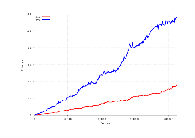
Figure 1. Isogeny computations for Jacobians of genus $2$ and $3$ curves in $\mathbb{F}_{7}$.

References

- [BCG+17] A. Bostan, F. Chyzak, M. Giusti, R. Lebreton, G. Lecerf, B. Salvy, and É. Schost. Algorithmes efficaces en calcul formel. 2017.
- [BCP97] W. Bosma, J. Cannon, and C. Playoust. The Magma algebra system. I. The user language. J. Symbolic Comput., 24(3-4):235–265, 1997. Computational algebra and number theory (London, 1993).
- [BGG+17] S. Ballentine, A. Guillevic, E. L. García, C. Martindale, M. Massierer, B. Smith, and J. Top. Isogenies for point counting on genus two hyperelliptic curves with maximal real multiplication. In Algebraic geometry for coding theory and cryptography, pages 63–94. Springer, 2017.
- [Car17] X. Caruso. Computations with -adic numbers. Les cours du CIRM, 5(1), 2017.
- [CE15] J.-M. Couveignes and T. Ezome. Computing functions on jacobians and their quotients. LMS Journal of Computation and Mathematics, 18(1):555–577, 2015.
- [CEL20] X. Caruso, E. Eid, and R. Lercier. Fast computation of elliptic curve isogenies in characteristic two. working paper or preprint, March 2020.
- [CR15] R. Cosset and D. Robert. Computing -isogenies in polynomial time on jacobians of genus 2 curves. Mathematics of Computation, 84(294):1953–1975, 2015.
- [CRV14] X. Caruso, D. Roe, and T. Vaccon. Tracking -adic precision. LMS J. Comput. Math., 17(suppl. A):274–294, 2014.
- [CRV15] X. Caruso, D. Roe, and T. Vaccon. -adic stability in linear algebra. In ISSAC’15—Proceedings of the 2015 ACM International Symposium on Symbolic and Algebraic Computation, pages 101–108. ACM, New York, 2015.
- [CS20] C. Costello and B. Smith. The supersingular isogeny problem in genus 2 and beyond. In International Conference on Post-Quantum Cryptography, pages 151–168. Springer, 2020.
- [FT19] E. V. Flynn and Y. B. Ti. Genus two isogeny cryptography. In J. Ding and R. Steinwandt, editors, Post-Quantum Cryptography, pages 286–306, Cham, 2019. Springer International Publishing.
- [GS12] P. Gaudry and É. Schost. Genus 2 point counting over prime fields. Journal of Symbolic Computation, 47(4):368–400, 2012.
- [KPR20] J. Kieffer, A. Page, and D. Robert. Computing isogenies from modular equations between Jacobians of genus 2 curves. working paper or preprint, January 2020.
- [LL06] R. Lercier and D. Lubicz. A quasi quadratic time algorithm for hyperelliptic curve point counting. The Ramanujan Journal, 12(3):399–423, 2006.
- [LS08] R. Lercier and T. Sirvent. On Elkies subgroups of -torsion points in elliptic curves defined over a finite field. J. Théor. Nombres Bordeaux, 20(3):783–797, 2008.
- [LV16] P. Lairez and T. Vaccon. On -adic differential equations with separation of variables. In Proceedings of the 2016 ACM International Symposium on Symbolic and Algebraic Computation, pages 319–323. ACM, New York, 2016.
- [Mat59] T. Matsusaka. On a characterization of a Jacobian variety. 1959.
- [Mil86] J. S. Milne. Abelian varieties. In Arithmetic geometry, pages 103–150. Springer, 1986.
- [Mil19] E. Milio. Computing isogenies between Jacobian of curves of genus 2 and 3. working paper or preprint, August 2019.
- [OS86] F. OORT and T. SEKIGUCHI. The canonical lifting of an ordinary jacobian variety need not be a jacobian variety. J. Math. Soc. Japan, 38(3):427–437, 07 1986.
- [Tho03] E. Thomé. Algorithmes de calcul de logarithmes discrets dans les corps finis. PhD thesis, École polytechnique, 2003.
- [Tia20] S. Tian. Translating the discrete logarithm problem on jacobians of genus 3 hyperelliptic curves with -isogenies, 2020.
- [Vac15] T. Vaccon. Précision p-adique: applications en calcul formel, théorie des nombres et cryptographie. PhD thesis, University of Rennes 1, 2015.