Lorentz Resonance in the Homogenization of Plasmonic Crystals

Abstract

We explain the Lorentz resonances in plasmonic crystals that consist of 2D nano dielectric inclusions as the interaction between resonant material properties and geometric resonances of electrostatic nature. One example of such plasmonic crystals are graphene nanosheets that are periodically arranged within a non-magnetic bulk dielectric. We identify local geometric resonances on the length scale of the small scale period. From a materials perspective, the graphene surface exhibits a dispersive surface conductance captured by the Drude model. Together these phenomena conspire to generate Lorentz resonances at frequencies controlled by the surface geometry and the surface conductance.

The Lorentz resonances found in the frequency response of the effective dielectric tensor of the bulk metamaterial is shown to be given by an explicit formula, in which material properties and geometric resonances are decoupled. This formula is rigorous and obtained directly from corrector fields describing local electrostatic fields inside the heterogeneous structure.

Our analytical findings can serve as an efficient computational tool to describe the general frequency dependence of periodic optical devices. As a concrete example, we investigate two prototypical geometries composed of nanotubes and nanoribbons.

1 Introduction

Novel frequency dependent electromagnetic behavior can be generated by patterned dispersive dielectric metamaterials undergoing localized geometric resonance. Here the period of the pattern lies below the wavelength of operation. Examples include plasmonic metasurfaces [42, 43], band gaps generated by periodic configurations of local plasmon resonators [34], and beam steering [29]. In this work we contribute to the analytic understanding of such periodic optical devices by investigating the role of local (frequency independent) geometric features and (frequency dependent) material properties. In particular, we explain the appearance of Lorentz resonances generated by periodically patterned dispersive dielectrics as the interaction between resonant material properties and local geometric resonances of electrostatic nature.

Concretely, we shall examine the optical frequency response of plasmonic crystals formed by 2D material inclusions (such as graphene) embedded in a non-magnetic bulk dielectric host. We use a Drude model for the local conductivity response of the 2D material but allow for a fairly general periodic geometry including, for example, graphene nanoribbons, or graphene nanotubes. In such geometries, frequency independent geometric resonances will be identified and characterized that occur on the length scale of the period of the 2D material inclusions. These local resonances are novel as they exist both on the surface of the sheets and in the bulk. Together with the dispersive surface conductance of the 2D material, both phenomena conspire to generate Lorentz resonances in the effective optical frequency response of the metamaterial. The resonance frequencies are controlled by the surface geometry and the surface conductance.

The Lorentz resonances for the effective dielectric tensor or equivalently the effective index of refraction for the bulk metamaterial are shown to be given by an explicit formula. This formula is rigorous and obtained directly from the corrector fields describing local electrostatic fields inside the heterogeneous structure. The local boundary value problem for the correctors follow from the periodic homogenization theory for Maxwell’s equations developed in [2, 17, 35, 36, 37]. The formula for the effective dielectric constant obtained here is notable in that the local geometric resonances and local surface conductivity are uncoupled. This offers the opportunity for efficient computation of the effective dielectric constant through the computation of the local geometric resonances that are independent of the specific material properties. The interaction between geometry and material dispersion is displayed explicitly in the rigorously derived formula.

In detail, our contributions with the current work can be summarized as follows:

• We describe the interplay between frequency-independent geometric nanoscale resonances and frequency-dependent local conductivity models that results in Lorentz resonances in the effective optical frequency response. We derive an explicit formula for the frequency response rigorously from a mathematical homogenization theory for Maxwell’s equations for periodic 2D material inclusions.

• The spectral decomposition is enabled by identifying an underlying compact self-adjoint operator on a proper function space. This was done by symmetrizing a non-hermitian operator.

• We discuss how to use the analytic result for computing approximations on the frequency response of periodic optical configurations. This approach offers a significant saving in computational resources because only one frequency-independent geometric eigenvalue problem has to be computed, in contrast to computing the corrector field for a huge number of fixed frequencies [17, 18].

• We examine two prototypical geometries—a nanotube, and a nanoribbon configuration—in more detail. The latter one is analytically and computationally much more challenging due to singularities at interior 2D material edges. We discuss decay estimates and examine the approximation quality of our computational approach.

1.1 Background: Homogenization of plasmonic crystals

The following analytical investigation is based on a rigorous periodic homogenization theory [2, 17, 35, 36, 37]. For the sake of simplicity, we will base our analytical investigation on a slightly simplified setting that we quickly outline here.

(a)

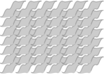
(b)

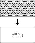
(c)

Figure 1: The homogenization procedure: (a) the nanoscale unit cell $Y$ consisting of 2D metallic inclusions $\Sigma$ with surface conductivity $\sigma(\omega)$ in an ambient host material with permittivity $\varepsilon$; (b) the plasmonic crystal formed by many scaled and repeated copies of $Y$ in every space dimension; (c) a schematic of the homogenization process in which the nanoscale structure is replace by a homogeneous material with effective permittivity $\varepsilon^{\text{eff}}$.

Consider a three-dimensional plasmonic crystal consisting of periodic copies of a representative volume element $Y$, which incorporates nanoscale inclusions given by 2D material surfaces (see Figure 1) of reasonably arbitrary shape (specified in Sec. 11.2 and Appendix B). The conductivity of the surfaces is assumed to obey the Drude model:

$$\sigma(\omega)\;=\;\frac{\textrm{i}\,\omega_{p}}{\omega+\textrm{i}/\tau},$$

where i denotes the imaginary unit, $\omega$ is the angular frequency, $\omega_{p}=4\,\alpha\approx 4/137$ is a (rescaled) Drude weight, and $\tau$ is a material-dependent relaxation time. Here, we have non-dimensionalized all quantities by applying a convenient rescaling [16]: $\tilde{\omega}=\frac{\hbar\omega}{E_{F}}$, where $E_{\text{F}}$ denotes the Fermi energy associated with the 2D material and $\hbar$ is the reduced Planck constant; $\tilde{\sigma}(\tilde{\omega})=\sqrt{\frac{\mu_{0}}{\varepsilon_{0}}}\,\sigma(\omega)$, where $\mu_{0}$ and $\varepsilon_{0}$ denote the vacuum permeability and permittivity, respectively. We set the length, height, and width of the representative volume element to one, $Y=[0,1]^{3}$. Furthermore, we assume that the dielectric host has a uniform and isotropic relative permittivity $\varepsilon$.

It can then be shown [17, 16] that for sufficiently small representative volume element $Y$ and sufficiently many repetitions of $Y$, i. e., a sufficiently large plasmonic crystal, the effective conductivity of the plasmonic crystal is given by a uniform, frequency-dependent conductivity tensor

(1) $$\varepsilon^{\text{eff}}_{ij}(\omega)\;=\;\varepsilon\,\delta_{ij}\;-\;\frac{\sigma(\omega)}{\textrm{i}\omega}\,\int_{\Sigma}\big{\{}P_{T}(\boldsymbol{e}_{j})\,+\,\nabla_{T}{\chi_{j}(\omega,\boldsymbol{x})}\big{\}}\cdot P_{T}(\boldsymbol{e}_{i})\,{\mathrm{d}}o_{x},\quad i,j=1,2,3.$$

Here, $\boldsymbol{x}$ represents the spatial coordinates, $\delta_{ij}$ is Kronecker’s Delta, $\boldsymbol{e}_{j}$ is the $j$-th unit vector, ${\Sigma}$ denotes the 2D material surface (embedded in $Y$), $P_{T}$ is the projection of a vector onto the two-dimensional tangential space of ${\Sigma}$, and $\nabla_{T}=P_{T}\nabla$ denotes the tangential gradient (with respect to ${\Sigma}$).

The $Y$-periodic corrector field $\boldsymbol{\chi}(\boldsymbol{x})$ for closed $\Sigma$ is the solution of the cell problem [17],

(2) $$\begin{cases}\begin{aligned} \Delta\chi_{j}(\boldsymbol{x})\big{)}&=0&&\text{in }Y\setminus\Sigma\leavevmode\nobreak\ ,\\[5.0pt] \left[\chi_{j}(\boldsymbol{x}))\right]_{{\Sigma}}&=0&&\text{on }\Sigma\leavevmode\nobreak\ ,\\[5.0pt] \varepsilon\left[\boldsymbol{\nu}\cdot\nabla\chi_{j}(\boldsymbol{x})\right]_{{\Sigma}}&=\frac{\sigma}{i\omega}\nabla_{T}\cdot\big{(}P_{T}\boldsymbol{e}_{j}+\nabla_{T}\chi_{j}(\boldsymbol{x})\big{)}&&\text{on }\Sigma\leavevmode\nobreak\ ,\color[rgb]{0,0,0}\end{aligned}\end{cases}$$

where, $\boldsymbol{\nu}$ is the unit outward normal of ${\Sigma}$ at $\boldsymbol{x}$, and $\left[f\right](\boldsymbol{x})$ denotes the jump of a quantity $f$ across the surface ${\Sigma}$ along the normal direction of ${\Sigma}$, viz.,

$$\left[f\right](\boldsymbol{x})\,:=\,\lim_{\alpha\searrow 0}\Big{(}f(\boldsymbol{x}+\alpha\boldsymbol{\nu})-f(\boldsymbol{x}-\alpha\boldsymbol{\nu})\Big{)}\quad\text{for }\boldsymbol{x}\in{\Sigma}.$$

The novelty of plasmonic materials is that they are used to control light at wavelengths much larger than the characteristic length scale of the period. Thus understanding wave dispersion for such systems through frequency-dependent effective behavior is quite natural. Recently frequency dependent effective dispersive behavior of a finite number of metallic sheets embedded in a dielectric host is compared to direct numerical simulation and shown to agree up to a negligible error [16]. In another work the frequency dependence of effective properties have been mathematically proven to deliver the leading-order dispersive behavior for subwavelength plasmonic composites, this is rigorously done in Theorem 4 of [7]. Last it is noted that the Lorentz resonance for a single particle is not sufficient for understanding periodic subwavelength patterned arrays of inhomogeneities as it ignores close range inter-particle interactions that are captured by the local fields that determine the effective dielectric constant.

1.2 Summary of the main result

The objective of our discussion is to decouple the frequency dependence introduced in (1) by the surface conductivity and other material parameters from the geometric resonances of the nanostructure. To this end we introduce an auxiliary spectral problem to identify all $\big{\{}\lambda_{n}\big{\}}\subset\mathbb{C}$ for which there exists a $\varphi_{n}$ satisfying

$$\begin{cases}\begin{aligned} \Delta\varphi_{n}(\boldsymbol{x})\big{)}&=0&&\text{in }Y\setminus\Sigma\leavevmode\nobreak\ ,\\[5.0pt] \left[\varphi_{n}(\boldsymbol{x}))\right]_{{\Sigma}}&=0&&\text{on }\Sigma\leavevmode\nobreak\ ,\\[5.0pt] \lambda_{n}\left[\boldsymbol{\nu}\cdot\nabla\varphi_{n}(\boldsymbol{x})\right]_{{\Sigma}}&=\nabla_{T}\cdot\nabla_{T}\varphi_{n}(\boldsymbol{x})&&\text{on }\Sigma\leavevmode\nobreak\ .\end{aligned}\end{cases}$$

Introducing $\eta(\omega)=\frac{\sigma(\omega)}{\textrm{i}\omega}$ we then show that the effective refractive index in (1) can be expressed by the formula

(3) $$\varepsilon^{\text{eff}}_{ij}(\omega)\;=\;\varepsilon\,\delta_{ij}\;-\;\eta(\omega)\,\int_{\Sigma}P_{T}(\boldsymbol{e}_{j})\cdot P_{T}(\boldsymbol{e}_{i})\,{\mathrm{d}}o_{x}\;-\;\sum_{n=1}^{\infty}\,\frac{\lambda_{n}\,\eta^{2}(\omega)}{\varepsilon-\lambda_{n}\,\eta(\omega)}\;M_{jn}\;\overline{M_{in}},$$

where the factors $M_{jn}$ are defined as

$$M_{jn}=\int_{\Sigma}P_{T}(\boldsymbol{e}_{j})\cdot\nabla_{T}\overline{\varphi}_{n}(\boldsymbol{x})\,{\mathrm{d}}o_{x},\quad j=1,2,3,\quad n=1,2,\ldots$$

The important property of this formula is that the integrals only depend on geometry, and the coefficients only depend on frequency. Equating the real part of the denominator in the coefficients of (3) to zero, recovers an explicit resonance frequency $\omega_{R,n}$ for which the contribution of the $n$-th term of the sum may become dominant,

$$\omega_{R,n}\;=\;\sqrt{\omega^{2}_{0,n}-1/(2\tau)^{2}},\quad\text{where}\;\;\omega^{2}_{0,n}\;=\;\frac{\lambda_{n}\omega_{p}}{\varepsilon},\qquad n=1,2,\ldots$$

1.3 Past works

Plasmonic crystals based on patterned dispersive dielectric 2D material inclusions has made possible an unprecedented wealth of novel functional optical devices [33, 19, 31, 25, 28, 40]. Possible applications range from optical holography [39], tunable metamaterials [27], and cloaking [1], to subwavelength focusing lenses [8].

The analytical approach taken here is motivated by earlier observations of local resonances occurring at the length scale of the microgeometry. Electrostatic resonances identified at the length scale of composite geometry were shown to control the effective dielectric responce associated with crystals made from non-dispersive dielectric inclusions in the pioneering work of [5] and [21]. The associated representation formulas based on local resonances were extended and applied to bound the effective dielectric response [23], [10], and [24]. Most recently local electrostatic and plasmonic resonances are used to construct non-magnetic double negative metamaterials in the near infrared [7] and design photonic band gap materials [13].

The current work advances the understanding of effective dielectric behavior by discovering and subsequently taking advantage of local resonances supported both on surfaces and in the bulk for generating Lorentz resonances at frequencies explicitly controlled by the microstructure.

1.4 Paper organization

The remainder of the paper is organized as follows. In Section 2 we introduce the analytical setting and discuss our spectral decomposition result. The emerging Lorentz resonance and an application to inverse optical design in discussed in Section 3. A computational framework based on the spectral decomposition is outlined in Section 4 and two prototypical geometries are computationally analyzed. We discuss implications and conclude in Section 5.

Analytical technicalities concerning the spectral decomposition result on closed and open surfaces are outlined in Appendices A and B. We summarize some explicit analytical formulas for the solution of the geometric eigenvalue problem in Appendix C.

2 Spectral Decomposition

In this section we introduce and characterize an auxiliary spectral problem that enables us to derive the spectral decomposition (3) of the cell problem (2). For the sake of argument we keep the discussion in this section on a formal level. A mathematically rigorous formulation of the spectral decomposition for general classes of closed and open 2D dielectric inclusions ${\Sigma}$ is given in Appendix A and B, respectively. Here, a closed inclusion $\Sigma$ is a $Y$-periodic two-dimensional surface that does not have any one-dimensional edges in the interior of $Y$. Similarly, an open inclusion $\Sigma$ is a $Y$-periodic two-dimensional surface that exhibit an edge in the interior of $Y$; see Figure 1.

2.1 An auxiliary eigenvalue problem

As a first step we introduce an auxiliary eigenvalue problem that is closely related to the cell problem (2) of the homogenization process. By removing the forcing $P_{T}\boldsymbol{e}_{j}$ and replacing the quotient $\tfrac{\textrm{i}\omega\varepsilon}{\sigma}$ by a real-valued eigenvalue $\lambda$ one arrives at the spectral problem: Find all pairs of eigenvalues $\lambda\in\mathbb{R}$ and corresponding square-integrable eigenfunctions $\varphi$ such that

(4) $$\begin{cases}\begin{aligned} \Delta\varphi(\boldsymbol{x})&=0&&\text{in }Y\setminus\Sigma\leavevmode\nobreak\ ,\\[5.0pt] \left[\phi(\boldsymbol{x})\right]_{{\Sigma}}&=0&&\text{on }\Sigma\leavevmode\nobreak\ ,\\[5.0pt] \lambda\left[\boldsymbol{\nu}\cdot\nabla\varphi(\boldsymbol{x})\right]_{{\Sigma}}&=\,\Delta_{T}\varphi(\boldsymbol{x})&&\text{on }\Sigma\leavevmode\nobreak\ .\end{aligned}\end{cases}$$

Here, $\boldsymbol{\nu}$ is again the unit outward normal of ${\Sigma}$ at $\boldsymbol{x}$. We have set $\,\Delta_{T}:=\nabla_{T}\cdot\nabla_{T}$ and $\left[f\right](\boldsymbol{x})$ denotes the jump of a quantity $f$ across the surface ${\Sigma}$ along the normal direction of ${\Sigma}$, viz.,

$$\left[f\right](\boldsymbol{x})\,:=\,\lim_{\alpha\searrow 0}\Big{(}f(\boldsymbol{x}+\alpha\boldsymbol{\nu})-f(\boldsymbol{x}-\alpha\boldsymbol{\nu})\Big{)}\quad\text{for }\boldsymbol{x}\in{\Sigma}.$$

Eigenvalue problem (4) is certainly well posed and will admit an orthonormal basis of square-integrable eigenfunctions provided one can identify an underlying self-adjoint and compact linear operator. For all square-integrable densities $\gamma(\boldsymbol{x})$ defined on the surface ${\Sigma}$ we thus introduce the periodic single layer operator $\mathbb{S}\gamma$ by setting

(5) $$(\mathbb{S}\gamma)(\boldsymbol{x}):=\int_{\Sigma}G_{\text{per}}(\boldsymbol{x}-\boldsymbol{y})\gamma(\boldsymbol{y})\,{\mathrm{d}}o_{y},\quad\boldsymbol{x}\in Y.$$

Here, $G_{\text{per}}$ is the periodic Green’s function of the periodic Laplace problem, viz.,

$$G_{\text{per}}(\boldsymbol{x}):=\sum_{\boldsymbol{z}\in\mathbb{Z}^{n}}G_{0}(\boldsymbol{z}+\boldsymbol{x}),\qquad G_{0}(x):=-\frac{1}{4\pi|x|}.$$

The single layer operator $\mathbb{S}$ is constructed in such a way that $\mathbb{S}\gamma$ satisfies

(6) $$\Delta\mathbb{S}\gamma=0\quad\text{in }\Omega\setminus{\Sigma},\qquad\left[\mathbb{S}\gamma\right]_{{\Sigma}}=0\quad\text{on }{\Sigma},\qquad\left[\boldsymbol{\nu}\cdot\nabla(\mathbb{S}\gamma)\right]_{{\Sigma}}=\gamma\quad\text{on }{\Sigma}.$$

An important insight (that we outline in Appendix A) is the fact that this process can be reversed: In particular, for every eigenfunction $\varphi$ that solves (4) one can find a density $\gamma$ such that $\varphi(\boldsymbol{x})=(\mathbb{S}\gamma)(\boldsymbol{x})$. This allows us to substitute the representation $\varphi=\mathbb{S}\gamma$ into the last equation of (4):

$$\lambda\gamma(\boldsymbol{x})\;=\;\,\Delta_{T}(\mathbb{S}\gamma)(\boldsymbol{x})\quad\text{on }\Sigma.$$

Let $S$ denote the single layer operator $\mathbb{S}$ restricted to ${\Sigma}$ and set $\xi=S\gamma$. Provided that the inverses $S$ and $\,\Delta_{T}^{-1}$ exist we can further rearrange the eigenvalue problem (4) into an equivalent spectral problem:

(7) $$\,\Delta_{T}^{-1}S^{-1}\xi\;=\;\lambda^{-1}\xi\leavevmode\nobreak\ .$$

We establish in Appendix A that for the case of closed surfaces $\Sigma$ both inverses $S^{-1}$ and $\,\Delta_{T}^{-1}$ do indeed exist and that the operator $\,\Delta_{T}^{-1}S^{-1}$ is compact and self adjoint on a modified Hilbert space

$$N({\Sigma})\;:=\;\left\{\xi\in H^{1}({\Sigma})\;:\;\int_{{\Sigma}}S^{-1}\xi\,{\mathrm{d}}o_{x}=0\right\},$$

with associated norm $\|\nabla_{T}\cdot\|_{L^{2}(\Sigma)}$. Here, $H^{1}({\Sigma})$ denotes the Sobolev space of square integrable functions with square-integrable generalized derivatives. In summary, this guarantees the existence of a countable set of real eigenvalues $\{\lambda_{n}^{-1}\}$, $n=1\color[rgb]{0,0,0}$, $2$, …converging to zero, and an associated orthonormal basis of eigenvectors $\{\xi_{n}\}$ of $N({\Sigma})$. Note that by design $\xi_{n}$ is precisely the restriction of $\varphi_{n}$ as characterized by (4) to the surface ${\Sigma}$.

2.2 Spectral characterization of the corrector

Consider now the $Y$-periodic corrector field $\chi(\boldsymbol{x})$, described by the cell problem (2). The aforementioned orthonormal basis of eigenvectors $\{\xi_{n}\}$ admits (up to a constant) a representation

$$\chi_{j}(\boldsymbol{x})=\sum_{n=1}^{\infty}\alpha^{n}_{j}\xi_{n}(\boldsymbol{x})\quad\text{on }\Sigma.$$

Substituting this characterization back into (2) and a bit of algebra exploiting (7) then yields an explicit formula for the coefficients:

(8) $$\alpha_{j}^{n}\;=\;\frac{\lambda_{n}\eta(\omega)}{\varepsilon-\lambda_{n}\,\eta(\omega)}\int_{\Sigma}P_{T}(\boldsymbol{e}_{j})\cdot\nabla_{T}\overline{\xi}_{n}\,{\mathrm{d}}o_{x},\qquad\eta(\omega)\;:=\;\frac{\sigma(\omega)}{\textrm{i}\omega},\qquad j=1,2,3.$$

Similarly, repeating the substitution for Equation (2) yields an explicit formula for the frequency behavior of the effective dielectric tensor:

(9) $$\varepsilon^{\text{eff}}_{ij}(\omega)\;=\;\varepsilon\,\delta_{ij}\;-\;\eta(\omega)\,\int_{\Sigma}P_{T}(\boldsymbol{e}_{j})\cdot P_{T}(\boldsymbol{e}_{i})\,{\mathrm{d}}o_{x}\;-\;\sum_{n=1}^{\infty}\,\frac{\lambda_{n}\,\eta^{2}(\omega)}{\varepsilon-\lambda_{n}\,\eta(\omega)}\;M_{jn}\;\overline{M_{in}},$$

where the factors $M_{jn}$ are defined as

$$M_{jn}=\int_{\Sigma}P_{T}(\boldsymbol{e}_{j})\cdot\nabla_{T}\overline{\varphi}_{n}(\boldsymbol{x})\,{\mathrm{d}}o_{x},\quad j=1,2,3,\quad n=1,2,\ldots$$

A number of remarks are in order. Eq. (9) separates the frequency dependence of the surface conductivity (included in $\eta(\omega)$ ) from the fundamental (frequency independent) geometric resonances described by eigenvalue problem (4) that determine eigenvalues $\lambda_{k}$ and eigenmodes $\xi_{k}$. This implies that material properties and geometric resonances, that both contribute to the frequency response of the effective permittivity tensor $\varepsilon^{\text{eff}}_{ij}(\omega)$, are decoupled: The spectrum $\lambda_{k}$ and eigenmodes $\xi_{k}$ of (4) only depend on the (nanoscale) geometry and not on the concrete surface conductivity model.

3 Macroscale frequency response

We now investigate the effective permittivity tensor $\varepsilon^{\text{eff}}(\omega)$ given by (9) further: First, the somewhat hidden Lorentz resonance structure in the coefficients of the sum in Eq. (9) is made explicit. We then discuss how Eq. (9) can be used to facillitate the inverse design process [22, 26].

3.1 Lorentz dispersive material

From (9) we see that resonances in the temporal behavior of the tensor emerge whenever the denominator in the coefficients of the sum is close to zero. Equating the real part of the denominator of

$$\frac{\lambda_{n}\eta^{2}(\omega)}{\varepsilon-\lambda_{n}\eta(\omega)}$$

to zero recovers a critical frequency

(10) $$\omega_{0,n}^{2}\;=\frac{\lambda_{n}\omega_{p}}{\varepsilon}.$$

Here, we assumed a simply Drude model $\sigma(\omega)=\frac{\textrm{i}\omega_{p}}{\omega+\textrm{i}/\tau}$ to hold, where $\omega_{p}\approx\frac{4}{137}$ is a rescaled Drude weight and $\tau$ is a material-dependent relaxation time. With this definition in place we can further manipulate the coefficients:

$$\frac{\lambda_{n}\eta^{2}(\omega)}{\varepsilon-\lambda_{n}\eta(\omega)}\;=\;\frac{\omega_{0,n}^{2}\omega_{p}}{\omega(\omega+\textrm{i}/\tau)}\;\cdot\;\frac{1}{\omega^{2}-\omega_{0,n}^{2}+\textrm{i}\omega/\tau}\,.$$

In general, the angular frequency $\omega$ is much larger than the inverse of the relaxation time, viz., $\omega\gg 1/\tau$. Thus, close to resonance we can reasonably assume that $\omega\approx\omega+\textrm{i}/\tau\approx\omega_{0,n}$ and obtain

$$\frac{\lambda_{n}\eta^{2}(\omega)}{\varepsilon-\lambda_{n}\eta(\omega)}\;\approx\;\omega_{p}\;\frac{1}{\omega^{2}-\omega_{0,n}^{2}+\textrm{i}\omega/\tau}\;=\;-\omega_{p}\;\frac{\big{(}\omega_{0,n}^{2}-\omega^{2}\big{)}-\textrm{i}\omega/\tau}{\big{(}\omega_{0,n}^{2}-\omega^{2}\big{)}^{2}+\omega^{2}/\tau^{2}}.$$

The coefficients are thus Lorentzian with resonance frequency

(11) $$\omega_{R,n}\;=\;\sqrt{\omega^{2}_{0,n}-1/(2\tau)^{2}},\qquad n=1,2,\ldots$$

In summary, we obtain that up to a constant:

$$\varepsilon^{\text{eff}}_{ij}(\omega)\;\sim\;\;M_{jn}\overline{M_{in}}\,\omega_{p}\;\frac{\big{(}\omega_{0,n}^{2}-\omega^{2}\big{)}-\textrm{i}\omega/\tau}{\big{(}\omega_{0,n}^{2}-\omega^{2}\big{)}^{2}+\omega^{2}/\tau^{2}},\quad\text{for}\;\omega\approx\omega_{R,n}.$$

We point out that the nanoscale geometry that determines the spectrum $\lambda_{n}$ and eigenmodes $\xi_{n}$ only influences the numerical values of the resonance frequencies $\omega_{0,n}$ and $\omega_{R,n}$ as well as the numerical values of the weights $M_{in}$.

In summary, this heuristic argument suggests that the macroscale optical response of the plasmonic crystal is that of a Lorentz dispersive material [14, 12, 6]: The frequency response of the effective permittivity, $\varepsilon^{\text{eff}}(\omega)$, can be approximated by a finite sum of Lorentz resonances, with explicit formulas for resonant frequencies and coefficients provided by our characterization (9).

3.2 Inverse optical design

The rational expression for the effective property given by (9) lends itself to an inverse optimal design paradigm for a desired dispersive response. Equation (9) shows that the location of the poles and zeros are controlled by the eigenvalues $\lambda_{n}$ and eigenfunctions $\zeta_{n}$. These depend on the radius of the nano tubes or the side-length of the nano ribbon. One can compute a library of $\lambda_{n}$ and $\zeta_{n}$ near the desired operating frequency for a range of geometric parameters. From this library one can pick the poles and zeros that delivers the dispersive response closest to the desired one. Here the focus is on manufacturable designs and future investigations will investigate libraries of manufacturable geometries to provide a manufactorable range of resonant response.

4 Computational platform

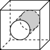
(a)

(b)

Figure 2: Prototypical geometries: (a) shows a nanotube configuration and (b) is a nanoribbon configuration. The diameter (in (a)) and the width (in (b)) was set to 0.8.

The spectral decomposition discussed in Section 22.2 allows for a very efficient computation of the frequency response of a nanostructure by first solving a single geometric eigenvalue problem given by (4) approximately. Then, (9) can be invoked to characterize the frequency response of the permittivity tensor. We will illustrate this procedure in this section on two prototypical geometries shown in Figure 2: a nanotube configuration, which is a closed smooth surface; and a nanoribbon configuration which is an open surface with edges. We point out that due to the translation invariance in $z$-direction of both configuration, the corresponding corrector $\boldsymbol{\chi}_{3}$ vanishes. This implies that the corresponding cell problems (13) reduce to a two-dimensional problem, and that the third diagonal component of the effective conductivity tensor $\varepsilon^{\text{eff}}$ is simply given by

$$\varepsilon^{\text{eff}}_{33}\;=\;\varepsilon\;-\;\eta(\omega)\,\int_{\Sigma}1\,{\mathrm{d}}o_{x}.$$

Due to symmetry we have $\varepsilon^{\text{eff}}_{11}=\varepsilon^{\text{eff}}_{22}$ for the nanotube configuration. In case of the nanoribbon geometry the averaging process in $y$-direction is trivial leading to $\varepsilon^{\text{eff}}_{22}=\varepsilon$. We thus only need to determine $\varepsilon^{\text{eff}}_{11}$ computationally in the following.

4.1 Numerical computation of the geometric spectrum

order k	$\lambda_{k}$	$\Big{|}\int_{{\Sigma}}P_{T}(\boldsymbol{e}_{1})\cdot\nabla_{T}\overline{\xi}_{n}\,{\mathrm{d}}o_{x}\Big{|}$
1	0.5924	1.1158
2	3.726	0.1077
3	6.289	0.008194
4	8.763	0.003574
5	11.26	0.0002755
6	13.76	0.00008546
7	16.27	0.000009443

(a) Nanotubes

$\lambda_{k}$	$\Big{|}\int_{{\Sigma}}P_{T}(\boldsymbol{e}_{1})\cdot\nabla_{T}\overline{\xi}_{n}\,{\mathrm{d}}o_{x}\Big{|}$
0.9873	0.8543
5.314	0.1811
9.283	0.1097
13.22	0.07913
17.16	0.06194
25.02	0.04322
28.96	0.03755

(b) Nanoribbons

Table 1: Numerically computed spectrum and weight coefficients for the two geometries (Figure 2) using the computational approach outlined in Section 3(a): Table (a) shows results for the nanotube configuration. All roots have multiplicity 2; eigenvalues with weight 0 are omitted. Table (b) shows shows results for the nanoribbon geometry. Here all roots have multiplicity 1.

In order to approximate (7) numerically we recast the eigenvalue problem in the variational form (4): Find $\varphi_{n}\in\mathcal{H}$ and $\lambda_{n}\in\mathbb{R}$ such that

$$\lambda_{n}\,\int_{Y}\nabla\varphi_{n}(\boldsymbol{x})\cdot\nabla\overline{\psi}(\boldsymbol{x})\,{\mathrm{d}}x\;=\;\int_{\Sigma}\nabla_{T}\varphi_{n}(\boldsymbol{x})\cdot\nabla_{T}\overline{\psi}(\boldsymbol{x})\,{\mathrm{d}}o_{x},\quad\forall\psi\in\mathcal{H}.$$

This eigenvalue problem can be efficiently approximated with a finite element discretization which we will quickly outline. We use the finite element toolkit deal.II [4, 3]. To achieve a good numerical convergence order we use unstructured quadrilateral meshes $\mathcal{T}_{h}$ for both geometries that are fitted to the curved hypersurface $\Sigma$ by aligning element boundaries with the hypersurface [15] and discretize with high-order Lagrange elements. Let $\big{\{}\psi^{h}_{i}\big{\}}_{i\in\{1:\mathcal{N}\}}$ be the nodal basis of the Lagrange ansatz. We can then define the usual stiffness matrix $M=(m_{ij})$

$$m_{ij}\;=\;\sum_{Q\in\mathcal{T}_{h}}\int_{Q}\nabla\psi^{h}_{j}(\boldsymbol{x})\cdot\nabla\psi^{h}_{i}(\boldsymbol{x})\,{\mathrm{d}}x.$$

The boundary term requires a modification because the trace $\nabla_{T}\psi^{h}_{i}$ is not single-valued and only defined on an individual cell of the mesh. We thus define a matrix $S=(s_{ij})$ by averaging both cell contributions to the gradient:

$$s_{ij}\;=\;\sum_{Q\in\mathcal{T}_{h}}\frac{1}{2}\int_{\partial Q}\nabla_{T}\psi^{h}_{j}(\boldsymbol{x})\cdot\nabla_{T}\psi^{h}_{i}(\boldsymbol{x})\,{\mathrm{d}}o_{x}.$$

We can then compute an approximate spectrum $\lambda_{n}^{h}$ and discrete eigenfunctions $\xi^{h}_{n}=\sum_{i}\Xi_{n,i}^{h}\psi^{h}_{i}$ by solving the matrix eigenvalue problem

$$\big{(}S+bM\big{)}\,\Xi_{n}^{h}\;=\;\tilde{\lambda}_{n}^{h}\,M\,\Xi_{n}^{h},\color[rgb]{0,0,0}$$

with an eigenvalue solver, such as SLEPc [11]. Here, $b>0$ is a suitably chosen Moebius parameter. The original eigenvalue is recovered via by setting $\lambda_{n}^{h}=\tilde{\lambda}_{n}^{h}-b$. We briefly comment on one crucial subtlety of this approach. The discrete eigenvectors $\Xi^{h}_{n}$ are orthonormal with respect to the inner product $\langle M\,.\,,\,.\,\rangle$ due to the mass matrix $M$ appearing on the right hand side. This inner product is the discrete analogue of $\int_{Y}\nabla\,.\cdot\nabla\,.\,{\mathrm{d}}x$ and not the normalization we used in Section 2. This does not change the computed eigenvalues but has an effect on the surface integrals that have to be computed next; see Proposition B.6 and the discussion in Appendix B. This can be easily cured by scaling the surface integrals appropriately by $1/\sqrt{\lambda^{h}_{n}}$, cf. Equations (9) and (21). We report numerical results for the two geometries (Figure 2) in Table 1. The decay rate of the weight coefficients $\Big{|}\int_{{\Sigma}}P_{T}(\boldsymbol{e}_{1})\cdot\nabla_{T}\overline{\xi}_{n}\,{\mathrm{d}}o_{x}\Big{|}$ deserves a short discussion. The rapid convergence of the coefficients to zero in case of nanotubes is owed to the regularity of ${\Sigma}$ and the absence of interior edges. The eigenvalues and eigenfunctions of the nanotube geometry can be explicitly computed when the periodic boundary condition on $Y$ is replaced by an infinite domain and the Sommerfeld radiation condition (see Appendix C). In this case only the first order, viz. $k=1$, has a nonzero contribution to the resonance. The rapid decay of the weight coefficients in our numerical result for the periodic case is qualitatively in agreement with this observation. Due to the singularities at the corners of the nanoribbon geometry [30], it is not surprising that the decay rate of the weight coefficients is limited.

An $n$-th order numerical approximation of the effective permittivity tensor can be constructed by invoking a discrete counterpart of (9):

(12) $$\varepsilon^{\text{app}}_{11}(\omega)\;=\;\varepsilon\,\;-\;\eta(\omega)\,\sum_{Q\in\mathcal{T}_{h}}\sum_{\partial Q\cap{\Sigma}}P_{T}(\boldsymbol{e}_{1})\cdot P_{T}(\boldsymbol{e}_{1})\,{\mathrm{d}}o_{x}\\[-10.00002pt] \;-\;\sum_{n=1}^{N}\,\frac{\lambda_{n}^{h}\eta^{2}(\omega)}{\varepsilon-\lambda_{n}^{h}\,\eta(\omega)}\;\left|\sum_{Q\in\mathcal{T}_{h}}\sum_{\partial Q\cap{\Sigma}}P_{T}(\boldsymbol{e}_{1})\cdot\nabla_{T}\xi^{h}_{n}\,{\mathrm{d}}o_{x}\right|^{2}.$$

4.2 Comparison

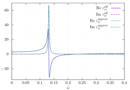
(a)

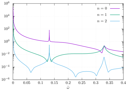
(b)

Figure 3: (a) Frequency response of $\varepsilon^{\text{eff}}_{ii}(\omega)$, $i=1,2$, for the nanotube configuration: The solid (real part) and dashed lines (imaginary part) are computed by solving the cell problem (2) for every $\omega$; the dotted and dash-dotted lines are computed by formula (9) truncated at $n=2$. (b) The corresponding relative error as a function of frequency.

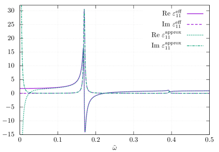
(a)

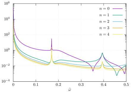
(b)

Figure 4: (a) Frequency response of $\varepsilon^{\text{eff}}_{11}(\omega)$, for the nanoribbon configuration: The solid (real part) and dashed lines (imaginary part) are computed by solving the cell problem (2) for every $\omega$; the dotted and dash-dotted lines are computed by formula (9) truncated at $n=2$. (b) The corresponding relative error as a function of frequency.

Choosing $\varepsilon=1$, we compute a reference frequency response of $\varepsilon^{\text{eff}}_{11}(\omega)$ by finely sampling over a set frequency range $0<\omega<0.5$ and performing a complete direct numerical computation of the cell problem for selected frequencies: For every chosen angular frequency $\omega$ we first determine the corrector by solving (2) with a finite-element code [18] up to a suitable resolution (about 110 k unknowns for the nanotube configuration, and about 130 k unknowns for the nanoribbon configuration). The result is plotted in Figures 3a and 4a. In both plots about 700 frequencies were chosen adaptively.

We then compare a second order approximation $\varepsilon^{\text{app}}_{11}$ by using (12) with $n=2$ against the direct numerical computation graphically in Figures 3a and 4a. For the chosen frequency range we observe an excellent agreement of the approximative permittivity $\varepsilon^{\text{app}}_{11}$ with the reference computation in the “eyeball” norm.

A more detailed comparison of the frequency behavior of the relative error between both computations is given in Figures 3b and 4b, where also the dependence of the error on the order $n$ of the approximation (12) is visualized. On average we observe a relative error of less than $1\,\%$. We note that the maxima in the relative error naturally occur at corresponding Lorentz resonances and are dominated by the approximation error of the underlying finite element simulations. We observe an exponential decay of the relative error as a function of approximation order for the smooth nanotubes geometry (see Figure 3b). The corresponding convergence behavior for nanoribbons as shown in Figure 4b is significantly slower. This is owed to the fact that the edges in the nanoribbon geometry cause singularity in the solution of the cell problems thus limiting the approximation order [30].

5 Conclusion

In this paper, we analyzed the Lorentz resonances in plasmonic crystals that consist of 2D nano dielectric inclusions embedded in a nonmagnetic bulk. From the corrector field found in a rigorous homogenization theory (13), we derived an analytic expansion formula for the effective permittivity (3). This formula decouples the local geometric resonances and the material properties, and thus enables a very efficient approximation to compute the frequency response. This formula holds for inclusions of a large family of geometries, including closed surfaces (as shown in Section 2 and Appendix A) and open surfaces that can be completed into closed surfaces as shown in Appendix B.

We observe that up to a constant factor, the $n$th Lorentz resonance is described by

$$\frac{\lambda_{n}\eta^{2}(\omega)}{\varepsilon-\lambda_{n}\eta(\omega)}\;\approx\;\omega_{p}\;\frac{1}{\omega^{2}-\omega_{0,n}^{2}+\textrm{i}\omega/\tau}\;=\;-\omega_{p}\;\frac{\big{(}\omega_{0,n}^{2}-\omega^{2}\big{)}+\textrm{i}\omega/\tau}{\big{(}\omega_{0,n}^{2}-\omega^{2}\big{)}^{2}+\omega^{2}/\tau^{2}}.$$

We have also observed that a crucial quantity that determines the convergence speed of this expansion is the decay rate of a weight factor

$$\Big{|}M_{jn}\Big{|}\;=\;\Big{|}\int_{{\Sigma}}P_{T}(\boldsymbol{e}_{j})\cdot\nabla_{T}\overline{\xi}_{n}\,{\mathrm{d}}o_{x}\Big{|}^{2}.$$

The decay rate depends on the smoothness of the corrector, i. e., whether singularities due to roughness or edges are present in the cell problem. We have demonstrated that our spectral decomposition approach offers a significant saving in computational resources because only one frequency-independent geometric eigenvalue problem has to be computed, in contrast to computing the corrector field for a huge number of fixed frequencies.

Appendix A Spectral Decomposition for closed surfaces

We now give a mathematical rigorous prove of the spectral decomposition introduced in Section 2 through the use of a weak formulation. The mathematical proof involves simpler function spaces when the surface $\Sigma$ is closed. For this reason we first discuss the case of a closed surface and discuss the case of open surfaces based on the notion of fractional Sobolev spaces in Appendix B.

A.1 The weak formulation

Provided the surface $\Sigma$ is Lipschitz continuous (implying it admits a uniquely defined surface normal), the $Y$-periodic corrector field $\boldsymbol{\chi}(\boldsymbol{x})$ is the solution of the variational cell problem [17],

(13) $$\textrm{i}\omega\varepsilon\,\int_{Y}\nabla\chi_{j}(\omega,\boldsymbol{x})\cdot\nabla\overline{\psi(\boldsymbol{x})}\,{\mathrm{d}}x\;-\;\sigma(\omega)\,\int_{\Sigma}\nabla_{T}\chi_{j}(\omega,\boldsymbol{x})\cdot\nabla_{T}\overline{\psi(\boldsymbol{x})}\,{\mathrm{d}}o_{x}\\ \;=\;\sigma(\omega)\int_{\Sigma}P_{T}\big{(}\boldsymbol{e}_{j})\cdot\nabla_{T}\overline{\psi(\boldsymbol{x})}\,{\mathrm{d}}o_{x}.$$

The appropriate function space for the variational problem (13) is

(14) $$\mathcal{H}\;:=\;\Big{\{}\psi\in H^{1}_{\text{per}}(Y,\mathbb{C})\,:\,\nabla_{T}\psi\in L^{2}({\Sigma},\mathbb{C}),\;\;\int_{Y}\psi=0\Big{\}}.$$

Here, $H^{1}_{\text{per}}(Y)$ denotes the Sobolev space of periodic functions $u$ such that $u$ and its first order (distributional) partial derivatives are square integrable in $Y$, and $L^{2}({\Sigma})$ denotes the space of square-integrable functions on ${\Sigma}$. The space $\mathcal{H}$ equipped with the norm

$$\|\,\cdot\,\|_{\mathcal{H}}^{2}=\|\nabla\,\cdot\,\|^{2}_{Y}+\|\nabla_{T}\,\cdot\,\|^{2}_{\Sigma}$$

(and the corresponding inner product) is a Hilbert space. It can be shown that the corrector problem (13) admits a unique solution $\chi_{j}\in\mathcal{H}$ [2, 17, 35, 36, 37].

Thus the auxiliary spectral problem partitioning between the first two integrals in (13), parallel to (4), is to find all pairs of eigenfunctions $\varphi\in\mathcal{H}$ and eigenvalues $\lambda\in\mathbb{R}$, such that

(15) $$\lambda\,\int_{Y}\nabla\varphi\cdot\nabla\overline{\psi}\,{\mathrm{d}}x\;=\;\int_{{\Sigma}}\nabla_{T}\varphi\cdot\nabla_{T}\overline{\psi}\,{\mathrm{d}}o_{x}\quad\text{for all }\psi\,{\in\mathcal{H}}.$$

A.2 A density representation for the corrector

The corrector $\chi_{i}\in\mathcal{H}$ given by (13) can be characterized in terms of the $Y$-periodic single layer potential $\mathbb{S}$ (5) with a density $\gamma$. Recall that we have restricted the discussion to the case of ${\Sigma}$ without internal edges in $Y$. In this case, the following two properties hold:

1. The restricted single layer operator $S\;:\;L^{2}({\Sigma})\to H^{1}({\Sigma})$ defined by by (6) is a bounded, invertible operator with a bounded inverse.

2. The jump in the normal derivative of the solution $\chi_{i}\in\mathcal{H}$ of the cell problem (13) on the surface, $[\partial_{\boldsymbol{\nu}}\chi_{j}]_{{\Sigma}}$, is in $L^{2}({\Sigma})$, where $L^{2}({\Sigma})$ the space of square integrable functions on ${\Sigma}$.

A proof of (i) for the case of Lipschitz continuous $\Sigma$ can be found in [20, Thm. 7.17], and Property (ii) is a direct consequence of the standard trace theorems [9] and Property (i). Note that Properties (i) and (ii) do not hold when ${\Sigma}$ is an open surface (i.e., when $\Sigma$ has edges in the interior of $Y$; see Appendix B). Starting from (ii), we set

$$\gamma\;:=\;[\partial_{\boldsymbol{\nu}}\chi_{j}]\;\in L^{2}(\Sigma,\mathbb{C}).$$

Recalling (6) we observe that the difference $\chi_{j}-\mathbb{S}\gamma$ belongs to $H^{1}_{\text{per}}(Y,\mathbb{C})$ and its distributional Laplacian is zero everywhere in $Y$. Therefore,

$$\chi_{j}=\mathbb{S}\gamma+C,$$

where $C$ is a constant. This suggests the following lemma:

Lemma A.1.

For the corrector $\chi_{j}$ solving (13), there exists a unique $\gamma\in L^{2}({\Sigma},\mathbb{C})$ and a unique complex valued constant $C$, such that

(16) $$\chi_{j}=\mathbb{S}\gamma+C,\qquad\text{with }\int_{{\Sigma}}\gamma\,{\mathrm{d}}o_{x}\;=\;0.$$

Proof A.2.

We have already established existence. For the uniqueness, assume that we have two representations for $\chi_{j}$, viz. $\mathbb{S}\gamma_{1}+C_{1}=\mathbb{S}\gamma_{2}+C_{2}$. This implies that $\mathbb{S}(\gamma_{1}-\gamma_{2})$ is a constant in $Y$, and thus

$$\gamma_{1}-\gamma_{2}\;=\;[\partial_{\boldsymbol{\nu}}\mathbb{S}(\gamma_{1}-\gamma_{2})]=0\qquad\text{on }{\Sigma}.$$

It follows that $C_{1}$ and $C_{2}$ are also identical. Finally, note that $\Delta\mathbb{S}\gamma=0$ implies

(17) $$\int_{{\Sigma}}\gamma\,{\mathrm{d}}o_{x}=\int_{{\Sigma}}[\partial_{\boldsymbol{\nu}}\mathbb{S}\gamma]\,{\mathrm{d}}o_{x}=-\int_{Y\setminus{\Sigma}}\Delta\mathbb{S}\gamma dx=0.$$

A.3 An equivalent spectral problem and symmetrization

Utilizing the same argument again as in the preceding subsection (Appendix AA.2), for closed $\Sigma$ every eigenfunction $\varphi$ of the spectral problem (15) has a representation $\varphi=\mathbb{S}\gamma$, where $\gamma\in L^{2}(\Sigma)$. Substituting the representation $\varphi=\mathbb{S}\gamma$ into (4), we obtain an equivalent spectral problem for $\gamma$:

$$\lambda\,\int_{Y}\nabla\mathbb{S}\gamma\cdot\nabla\overline{\psi}\,{\mathrm{d}}x\;=\;\int_{{\Sigma}}\nabla_{T}\mathbb{S}\gamma\cdot\nabla_{T}\overline{\psi}\,{\mathrm{d}}o_{x},\quad\text{for all }\psi\,{\in\mathcal{H}}.$$

Integration by parts of the volume integral and (6) further transforms the eigenvalue problem to an eigenvalue problem described exclusively on ${\Sigma}$:

$$-\lambda\,\int_{{\Sigma}}\gamma\,\overline{\psi}\,{\mathrm{d}}o_{x}\;=\;\int_{{\Sigma}}\nabla_{T}S\gamma\cdot\nabla_{T}\overline{\psi}\,{\mathrm{d}}o_{x}\quad\text{for all }\psi\,\in\mathcal{H}.$$

Writing $\xi=S\gamma$, which is equivalent to $\gamma=S^{-1}\xi$ since $S\;:\;L^{2}({\Sigma})\to H^{1}({\Sigma})$ is invertible for closed $\Sigma$, we obtain

$$-\lambda\,\int_{{\Sigma}}S^{-1}\xi\,\overline{\psi}\,{\mathrm{d}}o_{x}\;=\;\int_{{\Sigma}}\nabla_{T}\xi\cdot\nabla_{T}\overline{\psi}\,{\mathrm{d}}o_{x},\quad\forall\psi\,{\in\mathcal{H}}.$$

A.4 A compact and self-adjoint operator

The property of the density function $\gamma$ in Lemma A.1 suggests that we work with the space

(18) $$N({\Sigma})\;:=\;\left\{\xi\in H^{1}({\Sigma})\;:\;\int_{{\Sigma}}S^{-1}\xi\,{\mathrm{d}}o_{x}=0\right\}.$$

A straightforward calculation shows that $N(\Sigma)$ equipped with the norm $\|\nabla_{T}\xi\|_{L^{2}({\Sigma})}$ is a Hilbert space. The Riesz representation theorem then establishes a particular inverse of the Laplace-Beltrami operator $\Delta_{T}$:

Lemma A.3.

For $f\in L^{2}({\Sigma})$ with $\int_{{\Sigma}}f\,{\mathrm{d}}o_{x}=0$, there exists a unique $g\in N({\Sigma})$, such that

$$\int_{{\Sigma}}\nabla_{T}g\cdot\nabla_{T}\overline{\psi}\,{\mathrm{d}}o_{x}\;=\;-\int_{{\Sigma}}f\overline{\psi}\,{\mathrm{d}}o_{x},\quad\text{for all }\psi\in N({\Sigma}).$$

Moreover, the solution $g$ is bounded, viz., $\|\nabla_{T}g\|_{L^{2}({\Sigma})}\leq C\|f\|_{L^{2}({\Sigma})}$. We will denote this solution operator by $\,\Delta_{T}^{-1}$.

We are now in a position to formulate and proof a central proposition and corollary.

Proposition A.4.

The operator

$$\,\Delta_{T}^{-1}S^{-1}\;:\;N({\Sigma})\;\rightarrow\;N({\Sigma})$$

is compact and self-adjoint. Moreover, $\text{ker}\,(\,\Delta_{T}^{-1}S^{-1})=\left\{0\right\}$.

Corollary A.5 (Spectrum).

The spectrum of $\,\Delta_{T}^{-1}S^{-1}$ consists of countably many nonzero eigenvalues $\big{\{}\lambda_{n}^{-1}\big{\}}_{n}$, only possibly accumulating at $0$. The corresponding eigenfunctions $\big{\{}\xi_{n}\big{\}}$ form an orthonormal basis of $N({\Sigma})$.

Proof A.6 (Proof of Proposition A.4).

$\Delta_{T}^{-1}S^{-1}$ is well defined and bounded by virtue of Assumption (i) and Lemma A.3. For any given $f,g\in N({\Sigma})$, it holds that

$$-\int_{{\Sigma}}\big{(}\nabla_{T}\,\Delta_{T}^{-1}S^{-1}f\big{)}\cdot\nabla_{T}g\,{\mathrm{d}}o_{x}\,=\,\int_{{\Sigma}}\big{(}S^{-1}f\big{)}g\,{\mathrm{d}}o_{x}\,=\,\int_{{\Sigma}}f\big{(}S^{-1}g\big{)}\,{\mathrm{d}}o_{x}\\ \,=\,-\int_{{\Sigma}}\nabla_{T}f\cdot\big{(}\nabla_{T}\,\Delta_{T}^{-1}S^{-1}g\big{)}\,{\mathrm{d}}o_{x}$$

Therefore, $\,\Delta_{T}^{-1}S^{-1}$ is self adjoint.

In order to establish compactness of $\Delta_{T}^{-1}S^{-1}$, we first fix a bounded sequence $g_{i}\in N({\Sigma})$. The image $u_{i}=\,\Delta_{T}^{-1}S^{-1}g_{i}$ is also a bounded sequence in $N({\Sigma})$. By Rellich’s lemma, there exists subsequence $u_{i_{k}}$ that is convergent in $L^{2}({\Sigma})$. Furthermore, we have

$$\int_{{\Sigma}}\nabla_{T}u_{i}\cdot\nabla_{T}u_{j}\,{\mathrm{d}}o_{x}\,=\,-\int_{{\Sigma}}S^{-1}g_{i}\,u_{j}\,{\mathrm{d}}o_{x}.$$

Thus $\nabla_{T}u_{i_{k}}$ converges componentwise in $L^{2}({\Sigma})$, which gives that $u_{i_{k}}$ converges in $N({\Sigma})$.

The last statement follows immediately from the fact that $S$ and $\,\Delta_{T}$ are bounded and invertible. Thus $\,\Delta_{T}^{-1}S^{-1}f\equiv 0$ immediately implies $f\equiv S\,\,\Delta_{T}0=0$.

A.5 Proof of the spectral decomposition result

Proof A.7 (Proof of (9)).

Let $\chi_{j}$ be the solution of (13). According to Lemma A.1 we can write $\chi_{j}$ as a single layer potential with a density $\gamma\in L^{2}({\Sigma})$ that satisfy $\int_{{\Sigma}}\gamma\,{\mathrm{d}}o_{x}=0$, viz.,

$$\chi_{j}\,=\,\mathbb{S}\gamma\,+\,C.$$

Using the invertibility of $S$ we obtain that for $\xi=S\gamma\in N({\Sigma})$,

$$\chi_{j}\,=\,\mathbb{S}\,S^{-1}\xi\,+\,C.$$

Corollary A.5 guarantees the existence of the expansion $\xi=\sum_{k}\alpha_{j}^{k}\xi_{k}$ with $\{\alpha_{j}^{n}\}_{n}\in\ell^{2}(\mathbb{C})$, which yields (up to a constant):

$$\chi_{j}=\mathbb{S}S^{-1}\Big{(}\sum_{k}\alpha^{k}_{j}\xi_{k}\Big{)}.$$

Identity (8) follows directly from substituting this expansion into (13) and testing with $\psi=\mathbb{S}S^{-1}\xi_{k}$:

$$\eta(\omega)\int_{{\Sigma}}P_{T}\big{(}\boldsymbol{e}_{j})\cdot\nabla_{T}\overline{\xi_{k}}\,{\mathrm{d}}o_{x}\; =\;\sum_{n}(\varepsilon\alpha_{j}^{n}/\lambda_{n}-\alpha_{j}^{n}\eta(\omega))\int_{\Sigma}\nabla_{T}\xi_{n}\cdot\nabla_{T}\overline{\xi_{k}}\,{\mathrm{d}}o_{x}$$

$$=\;\sum_{n}(\varepsilon\alpha_{j}^{n}/\lambda_{n}-\alpha_{j}^{n}\eta(\omega))\,\delta_{kn}$$

$$=\;\varepsilon\alpha_{j}^{k}/\lambda_{k}-\alpha_{j}^{k}\eta(\omega).$$

Finally, Identity (9) follows from a similar substitution using Eqs. (8) and (1).

Appendix B Spectral decomposition on open surfaces

When ${\Sigma}$ is an open surface, in the sense that ${\Sigma}$ has edges in the interior of $Y$, the property in Sec. 2A.2, $S\;:\;L^{2}({\Sigma})\to H^{1}({\Sigma})$ is invertible, no longer holds. A counter-example is the fact that in two dimensional space, the non-periodic single layer potential maps $\frac{1}{\sqrt{a-x^{2}}}$ to a constant function on the interval $[-a,a]$ [41]. This means that we cannot write $\chi_{j}=\mathbb{S}\gamma+C$ for some $\gamma\in L^{2}({\Sigma})$. However, this representation is valid for $\gamma$ defined in a proper fractional Sobolev space. Thus, modifying the argument to fractional Sobolev spaces makes it possible to obtain the same expansion (9).

In this appendix, we collect all necessary modifications to the argument outlined in Appendix A, provided that the mild assumptions hold true that ${\Sigma}$ has smooth boundary and ${\Sigma}$ can be completed into a closed smooth surface ${\Sigma_{\ast}}$.

B.1 Sobolev spaces on open surfaces

We give a definition of Sobolev spaces defined on open surfaces following the notations in [20]. First, on a closed $C^{k,1}$ surface ${\Sigma_{\ast}}$ in $\mathbb{R}^{n}$, where $k\geq 0$ and $n>0$ are integers, $H^{s}({\Sigma_{\ast}})$ is defined through charts and the Fourier transform for $s\in[-k-1,k+1]$ [20, P.98].

Let ${\Sigma}$ be an open subset of ${\Sigma_{\ast}}$, and, for simplicity, assume the boundary of ${\Sigma}$ is smooth. For every real number $s\in\mathbb{R}$, we define

$$H^{s}({\Sigma}) :=\left\{f:{\Sigma}\rightarrow\mathbb{C}\,|\,f\text{ has an extension }\tilde{f}\in H^{s}({\Sigma_{\ast}})\right\},$$

$$\tilde{H}^{s}({\Sigma}) :=\text{ closure of }C^{\infty}_{0}({\Sigma})\text{ in }H^{s}({\Sigma_{\ast}}).$$

It is shown in [20, Thm. 3.14, Thm. 3.29, Thm. 3.30] that when ${\Sigma}$ is a Lipschitz subset of ${\Sigma_{\ast}}$, for all $s\in\mathbb{R}$,

$$(\tilde{H}^{s}({\Sigma}))^{\prime}=H^{-s}({\Sigma}),$$

$$(H^{s}({\Sigma}))^{\prime}=\tilde{H}^{-s}({\Sigma}),$$

$$\tilde{H}^{s}({\Sigma})=\left\{f\in H^{s}({\Sigma_{\ast}})\,|\,\text{supp}f\subset\overline{{\Sigma}}\right\},$$

and for an integer $m\in[0,k+1]$,

$$H^{m}({\Sigma}) =\left\{f:{\Sigma}\rightarrow\mathbb{C}\,|\,f\text{ and its weak tangential derivatives up to order }m\text{ are in }L^{2}({\Sigma})\right\}.$$

Note that the above defined $H^{s}({\Sigma})$ and $\tilde{H}^{-s}({\Sigma})$ for $s\geq 0$ are the same as those defined in [38, 32].

B.2 Spectral decomposition

We can now modify the argument in Appendix A as follows. Since $\chi_{j}$ belongs to $H^{1}(Y)$, its distributional Laplacian is $0$, and $[\partial_{n}\chi_{j}]=0$ on ${\Sigma_{\ast}}\setminus{\Sigma}$, we obtain the standard result that

Lemma B.1.

For the corrector $\chi_{j}$ solving (13), there exists a unique $\gamma\in\tilde{H}^{-1/2}({\Sigma},\mathbb{C})$ and a unique constant $C$, such that

$$\chi_{j}=\mathbb{S}\gamma+C.$$

This $\gamma$ satisfies that $\int_{{\Sigma}}\gamma\,{\mathrm{d}}o_{x}=0$.

The mapping property of $S$ on $\tilde{H}^{-1/2}({\Sigma})$ is given by

Lemma B.2 ([38, 32]).

The single layer operator $S:\tilde{H}^{-1/2}({\Sigma})\rightarrow H^{1/2}({\Sigma})$ is bijective.

The proper Hilbert space to consider becomes

(19) $$\mathcal{N}({\Sigma})\;:=\;\left\{f\in H^{1/2}({\Sigma}),\;\langle S^{-1}f,1\rangle_{{\Sigma}}=0\right\},$$

equipped with the inner product $\langle-S^{-1}\xi,\,\eta\rangle_{{\Sigma}}$. Here, $\langle\cdot,\,\cdot\rangle_{{\Sigma}}$ is the $L^{2}({\Sigma})$ pairing, and we’ll refer to $\langle-S^{-1}\xi,\,\eta\rangle_{{\Sigma}}$ as the $S^{-1}$ inner product.

On this space, we consider the following inverse of $\,\Delta_{T}$.

Lemma B.3 (A particular inverse of $\,\Delta_{T}$).

For $f\in\tilde{H}^{-1}({\Sigma})$ with $\langle f,\,1\rangle_{{\Sigma}}=0$, there exists a unique $g\in H^{1}({\Sigma})$ with $\langle S^{-1}g,\,1\rangle_{{\Sigma}}=0$, such that

(20) $$-\langle f,\,\psi\rangle_{{\Sigma}}\;=\;\int_{{\Sigma}}\nabla_{T}g\cdot\nabla_{T}\overline{\psi}\,{\mathrm{d}}o_{x},\quad\text{for all }\psi\in H^{1}({\Sigma}).$$

Moreover, the solution $g$ of (20) is bounded, $\|g\|_{H^{1}({\Sigma})}\leq C\|f\|_{H^{-1}({\Sigma})}$. We will denote this solution operator by $\,\Delta_{T}^{-1}$.

Proof B.4.

Given $f\in\tilde{H}^{-1}({\Sigma})$ with $\langle f,1\rangle_{{\Sigma}}=0$, it follows from standard elliptic equation theory that there exists a unique $\tilde{g}\in H^{1}({\Sigma})$ with $\langle\tilde{g},1\rangle_{{\Sigma}}=0$, such that

$$-\int_{{\Sigma}}f\overline{\psi}\,{\mathrm{d}}o_{x}\; =\;\int_{{\Sigma}}\nabla_{T}\tilde{g}\cdot\nabla_{T}\overline{\psi}\,{\mathrm{d}}o_{x}\quad\forall\psi\in H^{1}({\Sigma}),$$

$$\|\tilde{g}\|_{H^{1}({\Sigma})}\; \leq\;C\|f\|_{\tilde{H}^{-1}({\Sigma})}.$$

Now let $g_{0}=S^{-1}1\in\tilde{H}^{-1/2}({\Sigma})$ and define the constant

$$C(\tilde{g})\;:=\;\langle S^{-1}\tilde{g},1\rangle_{{\Sigma}}/\langle S^{-1}1,1\rangle_{{\Sigma}}=\langle\tilde{g},g_{0}\rangle_{{\Sigma}}/\langle 1,g_{0}\rangle_{{\Sigma}}.$$

The function $g\,:=\,\tilde{g}-C(\tilde{g})$ obviously solves (20) and by construction $\langle S^{-1}g,1\rangle_{{\Sigma}}=0$. The bound follows from

$$\|C(\tilde{g})\|_{H^{1}}=\|C(\tilde{g})\|_{L^{2}}\leq C|\langle S^{-1}\tilde{g},1\rangle|\leq C\|S^{-1}\tilde{g}\|_{L^{2}}\leq C\|\tilde{g}\|_{H^{1}}\leq C\|f\|_{\tilde{H}^{-1}}.$$

Since $\,\Delta_{T}^{-1}S^{-1}$ maps $N({\Sigma})\subset H^{1/2}({\Sigma})$ into $H^{1}({\Sigma})\subset\subset H^{1/2}({\Sigma})$, we can verify:

Proposition B.5.

The operator

$$\,\Delta_{T}^{-1}S^{-1}\;:\;\mathcal{N}({\Sigma})\;\rightarrow\;\mathcal{N}({\Sigma})$$

is compact and self-adjoint with respect to the $S^{-1}$ pairing. Here $\,\Delta_{T}^{-1}$ is the particular operator defined in Lemma B.3. Moreover,

$$\text{ker}\,(\,\Delta_{T}^{-1}S^{-1})=\left\{0\right\}.$$

Finally, the main result reads:

Proposition B.6 (Spectral decomposition for open surfaces).

Let $\chi_{j}$ be the solution of the cell problem (13). Let $\{\xi_{n},\lambda_{n}^{-1}\}_{n}$ be the orthonormal eigen-system of the operator $\,\Delta_{T}S$ in the space $\mathcal{N}({\Sigma})$. Then

$$\chi_{j}=\mathbb{S}S^{-1}\Big{(}\sum_{n}\alpha^{n}_{j}\xi_{n}\Big{)}+C,$$

where $C$ is a constant and

$$\alpha_{j}^{n}\;=\;\frac{\eta(\omega)}{\varepsilon-\lambda_{n}\,\eta(\omega)}\int_{\Sigma}P_{T}(\boldsymbol{e}_{j})\cdot\nabla_{T}\overline{\xi}_{k}\,{\mathrm{d}}o_{x}.$$

Furthermore,

(21) $$\varepsilon^{\text{eff}}_{ij}\;=\;\varepsilon\,\delta_{ij}\;-\;\eta(\omega)\,\int_{{\Sigma}}P_{T}(\boldsymbol{e}_{j})\cdot P_{T}(\boldsymbol{e}_{i})\,{\mathrm{d}}o_{x}\\ \;-\;\sum_{n}\,\frac{\eta^{2}(\omega)}{\varepsilon-\lambda_{n}\,\eta(\omega)}\;\int_{{\Sigma}}P_{T}(\boldsymbol{e}_{j})\cdot\nabla_{T}\overline{\xi}_{n}\,{\mathrm{d}}o_{x}\;\int_{{\Sigma}}\nabla_{T}\xi_{n}\cdot P_{T}(\boldsymbol{e}_{i})\,{\mathrm{d}}o_{x}.$$

Note that the $S^{-1}$ inner product gives a different normalization of $\xi_{n}$ hence different $\alpha_{j}^{n}$ values. In terms of the scaled function $\tilde{\xi}_{k}:=\frac{\xi_{k}}{\sqrt{|\lambda_{k}|}}$, (4) is satisfied and the expansion (21) takes the same form as (3).

Appendix C Explicitly computable examples

We explicitly compute the eigensystem of $\,\Delta_{T}^{-1}S^{-1}$ on two nonperiodic geometries in $\mathbb{R}^{3}$. These examples qualitatively illustrate the corresponding periodic geometries, when the inclusions are far apart from each other. On spheres and circular cylinders in $\mathbb{R}^{3}$, the eigensystem of $\,\Delta_{T}S$ are explicitly known. This is because $\,\Delta_{T}$ and $S$ separately have explicit eigensystems, and they share eigenfunctions. Note that the only manifolds on which the Laplace-Beltrami operator has explicit eigensystems are $n$-spheres, $n$-tori and Heisenberg groups.

C.1 Circular cylinder

Let ${\Sigma}$ be a cylinder with a circular cross section of radius $a$. The corresponding periodic geometry is the nanotube structure considered numerically in Sec. 4. We will abuse notation by denoting the cross sections of all quantities by the same notation, since all quantities are invariant along the axis of the cylinder. A basis for mean zero $L^{2}(\Sigma)$ functions is $\left\{e^{in\theta},n\neq 0\right\}$. This is also a set of simultaneous eigen functions for $\,\Delta_{T}$ and $S$:

$$\,\Delta_{T}e^{in\theta}=-\frac{n^{2}}{a^{2}}e^{in\theta},\quad Se^{in\theta}=-\frac{a}{2n}e^{in\theta}.$$

Thus the eigensystem for (7) normalized in the $\|\nabla_{T}\cdot\|_{L^{2}({\Sigma})}$ norm is

$$\lambda_{n}=\frac{n}{2a},\quad\xi_{n}^{k\color[rgb]{0,0,0}}=\begin{cases}\frac{1}{n}\sqrt{\frac{a}{\pi}}\cos(n\theta),\quad k\color[rgb]{0,0,0}=1\\ \frac{1}{n}\sqrt{\frac{a}{\pi}}\sin(n\theta),\quad k\color[rgb]{0,0,0}=2\end{cases},\quad n\geq 1.$$

Using $P_{T}(\boldsymbol{e}_{1})=-\hat{\theta}\sin\theta$ and $\nabla_{T}=\hat{\theta}\frac{1}{a}\partial_{\theta}$, we obtain

$$\int_{\Sigma}P_{T}(\boldsymbol{e}_{1})\cdot\nabla_{T}\overline{\xi}_{n}^{k\color[rgb]{0,0,0}}\,{\mathrm{d}}o_{x}=\begin{cases}\sqrt{\pi a},\quad n=1,\,k=1,\\ 0,\quad\text{otherwise}.\end{cases}$$

Note that the for the corresponding periodic geometry, the factor $\int_{\Sigma}P_{T}(\boldsymbol{e}_{1})\cdot\nabla_{T}\overline{\xi}_{n}^{k\color[rgb]{0,0,0}}\,{\mathrm{d}}o_{x}$ in Table 1 decays, instead of falling to zero abruptly. This is due to the effect from other cylinders in the array. The decay becomes faster when the size of the cylinder relative to the cell becomes smaller.

C.2 Sphere

Let ${\Sigma}$ be a sphere of radius $a$. A basis for mean zero $L^{2}(\Sigma)$ functions is the set of spherical harmonic functions $\left\{Y_{n}^{m},n\geq 1,-n\leq m\leq n\right\}$. This is also a set of simultaneous eigenfunctions for $\,\Delta_{T}$ and $S$:

$$\,\Delta_{T}Y_{n}^{m}=-\frac{n(n+1)}{a^{2}}Y_{n}^{m},\quad SY_{n,m}=-\frac{a}{2n+1}Y_{n,m}.$$

Thus the eigensystem for (7) is normalized in the $\|\nabla_{T}\cdot\|_{L^{2}({\Sigma})}$ norm is

$$\lambda_{n}=\frac{n(n+1)}{a(2n+1)},\quad\xi_{n}^{i}=\frac{1}{\sqrt{n(n+1)}}Y_{n,m},\quad n\geq 1,-n\leq m\leq n.$$

Using $P_{T}(\boldsymbol{e}_{1})=\hat{\theta}\cos\theta\cos\phi-\hat{\phi}\sin\phi$, $\nabla_{T}=\hat{\theta}\frac{1}{a}\partial_{\theta}+\hat{\phi}\frac{1}{a\sin\theta}\partial_{\phi}$ and the recurrence relations for the associated Legendre polynomials, we obtain

$$\int_{\Sigma}P_{T}(\boldsymbol{e}_{1})\cdot\nabla_{T}\overline{\xi}_{n}^{i}\,{\mathrm{d}}o_{x}=\begin{cases}\mp 2a\sqrt{\frac{\pi}{3}},\quad n=1,\,m=\pm 1,\\ 0,\quad\text{otherwise}.\end{cases}$$

References

- [1] Andrea Alù and Nader Engheta. Achieving transparency with plasmonic and metamaterial coatings. Phys. Rev. E, 72:016623, Jul 2005.
- [2] Youcef Amirat and Valdimir V. Shelukhin. Homogenization of time harmonic Maxwell equations: the effect of interfacial currents. Mathematical Methods in the Applied Sciences, 40(8):3140–3162, 2017.
- [3] Daniel Arndt, Wolfgang Bangerth, Bruno Blais, Thomas C. Clevenger, Marc Fehling, Alexander V. Grayver, Timo Heister, Luca Heltai, Martin Kronbichler, Peter Munch, Matthias Maier, Jean-Paul Pelteret, Reza Rastak, Bruno Turcksin, Zhuoran Wang, and David Wells. The deal.II Library, Version 9.2. Journal of Numerical Mathematics, 28(3):131–146, 2020.
- [4] Daniel Arndt, Wolfgang Bangerth, Denis Davydov, Timo Heister, Luca Heltai, Martin Kronbichler, Matthias Maier, Jean-Paul Pelteret, Bruno Turcksin, and David Wells. The deal.II finite element library: design, features, and insights. Computers & Mathematics with Applications, 81(1):407–422, 2021.
- [5] David J. Bergman. The dielectric constant of a composite material - a problem in classical physics. Physics Reports, 43:377–407, 1978.
- [6] Max Born and Emil Wolf. Principles of optics: electromagnetic theory of propagation, interference and diffraction of light. Elsevier, 6th corrected edition, 2013.
- [7] Yue Chen and Robert Lipton. Resonanace and double negative behavior in metamaterials. Archive for Rational Mechanics and Analysis, 209:835–868, 2013.
- [8] Jierong Cheng, Wei Li Wang, Hossein Mosallaei, and Efthimios Kaxiras. Surface plasmon engineering in graphene functionalized with organic molecules: A multiscale theoretical investigation. Nano Letters, 14(1):50–56, 2014.
- [9] David Gilbarg and Neil S Trudinger. Elliptic partial differential equations of second order. springer, 2015.
- [10] Kennith Golden and George Papanicolaou. Bounds for effective parameters of heterogeneous media by analytic continuation. Commun, Math. Phys., 90:473–491, 1983.
- [11] Vicente Hernandez, Jose E. Roman, and Vicente Vidal. SLEPc: A scalable and flexible toolkit for the solution of eigenvalue problems. ACM Trans. Math. Software, 31(3):351–362, 2005.
- [12] Charles Kittel. Introduction to solid state physics. John Wiley and Sons, Inc., 8th edition, 2005.
- [13] Robert Lipton and Robert Viator. Bloch waves in crystals and periodic high contrast media. ESAIM Mathematical Modeling and Numerical Analysis, 51:889–918, 2017.
- [14] Hendrik Antoon Lorentz. The theory of electrons and its applications to the phenomena of light and radiant heat, volume 29. GE Stechert & Company, 1916.
- [15] Matthias Maier, Dionisios Margetis, and Mitchell Luskin. Dipole excitation of surface plasmon on a conducting sheet: finite element approximation and validation. J. Comp. Phys., 339:126–145, 2017.
- [16] Matthias Maier, Dionisios Margetis, and Mitchell Luskin. Finite-size effects in wave transmission through plasmonic crystals: A tale of two scales. Physical Review B, 102:075308, 2020.
- [17] Matthias Maier, Dionisios Margetis, and Antoine Mellet. Homogenization of time-harmonic maxwell’s equations in nonhomogeneous plasmonic structures. Journal of Computational and Applied Mathematics, page 112909, 2020.
- [18] Matthias Maier, Marios Mattheakis, Efthimios Kaxiras, Mitchell Luskin, and Dionisios Margetis. Homogenization of plasmonic crystals: Seeking the epsilon-near-zero effect. Proceedings of the Royal Society A: Mathematical, Physical, and Engineering Sciences, 475:20190220, 2019.
- [19] Marios Mattheakis, Constantinos A. Valagiannopoulos, and Efthimios Kaxiras. Epsilon-near-zero behavior from plasmonic dirac point: Theory and realization using two-dimensional materials. Physical Review B, 94:201404(R), 2016.
- [20] William McLean. Strongly elliptic systems and boundary integral equations. Cambridge University Press, 2000.
- [21] Ralph C. McPhedran and Graeme W. Milton. Bounds and exact theories for transport properties of inhomogeneous media. Applied Physics A., 26:207–220, 1981.
- [22] O.D. Miller and E. Yablonovitch. Inverse optical design. In B. Engquist, editor, Encyclopedia of Applied and Computational Mathematics, pages 729–732. Springer Berlin Heidelberg, Berlin, Heidelberg, 2015.
- [23] Graeme W. Milton. Bounds on the complex permittivity of a two-component composite material. J. Appl. Phys., 52:5286–5293, 1981.
- [24] Graeme W. Milton. The Theory of Composites. Cambridge University Press, Cambridge, 2002.
- [25] Parikshit Moitra, Yuanmu Yang, Zachary Anderson, Ivan I. Kravchenko, Dayrl P. Briggs, and Jason Valentine. Realization of an all-dielectric zero-index optical metamaterial. Nature Photonics, 7:791–795, 2013.
- [26] Sean Molesky, Zin Lin, Alexander Y. Piggott, Weiliang Jin, Jelena Vucković, and Alejandro W. Rodriguez. Inverse design in nanophotonics. Nature Photonics, 12:659–670, 2018.
- [27] Andrei Nemilentsau, Tony Low, and George Hanson. Anisotropic 2d materials for tunable hyperbolic plasmonics. Phys. Rev. Lett., 116:066804, 2016.
- [28] Xianxiang Niu, Xiaoyang Hu, Saisai Chu, and Qihung Gong. Epsilon-near-zero photonics: A new platform for integrated devices. Advanced Optical Materials, 6:1701292, 2018.
- [29] A. Pors, O. Albrektsen, I.P. Radko, and S.I. Bozhevonlnyi. A review of gap-surface plasmon metasurfaces: fundamentals and applications. Sci. Rep., 3:2155, 2013.
- [30] R. Rannacher and H. Blum. Extrapolation techniques for reducing the pollution effect of reentrant corners in the finite element method. Numerische Mathematik, 52(5):539–564, 1987/88.
- [31] Mario Silveirinha and Nader Engheta. Tunneling of electromagnetic energy through subwavelength channels and bends using epsilon-near-zero materials. Physical Review Letters, 97:157403, 2006.
- [32] Ernst P. Stephan. Boundary integral equations for screen problems in . Integral Equations and Operator Theory, 10:236–257, 1987.
- [33] Teng Tan, Xiantao Jiang, Cong Wang, Baicheng Yao, and Han Zhang. 2d material optoelectronics for information functional device applications: status and challenges. Advanced Science, 7(11):2000058, 2020.
- [34] R. Taubert, D. Dregely, T. Stroucken, A. Christ, and H. Giessen. Octave-wide photonic band gap in three-dimensional plasmonic bragg structures and limitations of radiative coupling. Nature Communications, 3:691, 2012.
- [35] Niklas Wellander. Homogenization of the Maxwell equations: Case i. linear theory. Applications of Mathematics, 46(1):29–51, 2001.
- [36] Niklas Wellander. Homogenization of the Maxwell equations: Case ii. nonlinear conductivity. Applications of Mathematics, 47(3):255–283, 2002.
- [37] Niklas Wellander and Gerhard Kristensson. Homogenization of the Maxwell equations at fixed frequency. SIAM Journal on Applied Mathematics, 64(1):170–195, 2003.
- [38] W. L. Wendland, E. Stephan, Darmstadt, and G. C. Hsiao. On thi integral equation method for the plane mixed boundary value problem of the laplacian. Mathemathical Methods in the Applied Sciences, 1(3):265–321, 1979.
- [39] Daniel Wintz, Patrice Genevet, Antonio Ambrosio, Alex Woolf, and Federico Capasso. Holographic metalens for switchable focusing of surface plasmons. Nano Letters, 15(5):3585–3589, 2015.
- [40] Fengnian Xia, Han Wang, Di Xiao, Madan Dubey, and Ashwin Ramasubramaniam. Two-dimensional material nanophotonics. Nature Photonics, 8:899–907, 2014.
- [41] Y. Yan and I. H. Sloan. On integral equations of the first kind with logarithmic kernels. Journal of integral equations and applications, 1(4):549–579, 1988.
- [42] Yang Zhao and Andrea Alù. Manipulating light polarization with ultrathin plasmonic metasurfaces. Physical Review B, 84(20):205428, 2011.
- [43] Yang Zhao, Xing-Xiang Liu, and Andrea Alù. Recent advances on optical metasurfaces. Journal of Optics, 16(12):123001, 2014.