Can neutron disappearance/reappearance experiments definitively rule out the existence of hidden braneworlds endowed with a copy of the Standard Model?

Abstract

Many works, aiming to explain the origin of dark matter or dark energy, consider the existence of hidden (brane)worlds parallel to our own visible world - our usual universe - in a multidimensional bulk. Hidden braneworlds allow for hidden copies of the Standard Model. For instance, atoms hidden in a hidden brane could exist as dark matter candidates. As a way to constrain such hypotheses, the possibility for neutron-hidden neutron swapping can be tested thanks to disappearance-reappearance experiments also known as passing-through-walls neutron experiments. The neutron-hidden neutron coupling $g$ can be constrained from those experiments. While $g$ could be arbitrarily small, previous works involving a $M_{4}\times R_{1}$ bulk, with DGP branes, show that $g$ then possesses a value which is reachable experimentally. It is of crucial interest to know if a reachable value for $g$ is universal or not and to estimate its magnitude. Indeed, it would allow, in a near future, to reject definitively - or not - the existence of hidden braneworlds from experiments. In the present paper, we explore this issue by calculating $g$ for DGP branes, for $M_{4}\times S_{1}/Z_{2}$, $M_{4}\times R_{2}$ and $M_{4}\times T^{2}$ bulks. As a major result, no disappearance-reappearance experiment would definitively universally rules out the existence of hidden worlds endowed with their own copy of Standard Model particles, excepted for specific scenarios with conditions reachable in future experiments.

I Introduction

The existence of hidden braneworlds coexisting with our universe in a multidimensional bulk is an open question often considered in the literature regarding the quest to explain the dark matter or dark energy conundrum art82 ; art76 ; art83 ; art84 ; art85 ; art77 ; art86 ; art87 . As a consequence, beyond cosmological tests or attempts for dark matter particle detection in astroparticle physics, any other search for direct evidence of hidden worlds is fundamental. In the last fifteen years, it has been theoretically shown that neutron swapping could occur between two adjacent braneworlds both endowed with a copy of the Standard Model of particles art65 ; art107 ; art4 ; art38 ; art50 . This phenomenology is related to the fact that any Universe with two braneworlds – i.e. two topological defects in the bulk – is equivalent to an effective noncommutative two-sheeted spacetime $M_{4}\times Z_{2}$ when one follows the dynamics of particles below the GeV-scale art4 . A neutron $n$ can convert into a hidden neutron $n^{\prime}$ propagating in a hidden neighboring braneworld with a probability $p\sim g^{2}$, where $g$ is the coupling constant between the two braneworlds art38 . As a result, new kind of experiments exploiting this phenomenon has been suggested in order to probe the braneworld hypothesis art40 ; art41 ; art5 ; art6 ; art24 . For instance, neutron disappearance (reappearance) toward (from) a hidden brane can be tested to constrain the coupling constant $g$ between the visible and hidden sectors. This is the case for instance with passing-through-walls neutron experiments carried out in the last five years art5 ; art6 ; art24 . Nevertheless, $g$ is a phenomenological constant which must depend on the brane energy scale (or its thickness), the interbrane distance, the bulk dimensionality and metrics art50 . As a consequence, knowing the behaviour of $g$ against these parameters is fundamental to put constraints on specific braneworld scenarios according to experimental data but also to plan future experiments and to determine their viability or relevance.

In a previous work art50 , we introduced a phenomenological approach to compute the coupling $g$ for two DGP braneworlds art80 ; art27 embedded in a $M_{4}\times R_{1}$ bulk with a warped Chung-Freese-like metric art29 ; art104 ; art105 . One obtained for the coupling $g$ between neutron and hidden neutron art50 :

$$g=(m^{2}/M_{B})\ e^{-md},$$ (1)

where $m$ is the mass of a constituent quark ($340$ MeV) art106 , $M_{B}$ the effective brane energy scale which is related to the thickness of the brane $M_{B}^{-1}$ with respect to the extra dimension and the ratio of the distortion factors of each brane and $d$ the interbrane distance.

In the present paper, using the same method, we calculate $g$ for various bulks and we discuss the consequences in regard of experimental data for the future experiments which can be considered and expected. In section II, we recall the low-energy framework used to describe a Universe with two braneworlds at least. In section III, the 5-dimensional case with a $S_{1}/Z_{2}$ compactified extra dimension is considered. This scenario has a historical interest since it is related to the 11D supergravity model of Hořava and Witten art31 . In section IV, the model is extended to 6 dimensions and the expression of $g$ related to two large extra dimensions is derived. The result is then extended to an ADD-like scenario art78 ; art79 – thanks to a compactification on a torus $T^{2}$ – in section V. Finally, in section VI, magnitudes of the coupling constant $g$ according to these different scenarios are discussed and crossed with experimental data in the context of next generation experiments.

II Low-energy description of a Universe with two braneworlds

The fermion dynamics in a two-braneworld system can be described at low energy as being the fermion dynamics in a $M_{4}\times Z_{2}$ noncommutative two-sheeted spacetime as demonstrated elsewhere art4 (see Fig. 1). The effective two spacetime sheets – without thickness – are separated by an effective distance $\xi=1/g$, where $g$ is the coupling constant between the fermions of each braneworld. In this $M_{4}\times Z_{2}$ spacetime, the gauge field $U(1)_{+}\times U(1)_{-}$ arises when considering the electromagnetic field. Both sheets – named $(+)$ and $(-)$ – are endowed with their own effective gauge field $U(1)_{+}$ and $U(1)_{-}$. This low energy description is valid whatever the mechanism responsible for the particle and fields trapping on the branes, the number of extra dimensions or the metric of the bulk art4 . The Lagrangian of the $M_{4}\times Z_{2}$ model is given by art4 ; art38 :

$$\mathcal{L}_{M_{4}\times Z_{2}}\sim\overline{\Psi}\left({i{\not{D}}_{A}-M}\right)\Psi,$$ (2)

where

$${i{\not{D}}_{A}-M}=\left(\begin{array}[]{cc}i\gamma^{\mu}(\partial_{\mu}+iqA_{\mu}^{+})-m&ig\gamma^{5}-im_{r}\\ ig\gamma^{5}+im_{r}&i\gamma^{\mu}(\partial_{\mu}+iqA_{\mu}^{-})-m\end{array}\right)$$ (3)

is typical of the noncommutative $M_{4}\times Z_{2}$ spacetime. For these two equations, $\Psi=\left(\begin{array}[]{c}\psi_{+}\\ \psi_{-}\end{array}\right)$ is a two-level spinor which contains the fermionic wave functions $\psi_{+}$ in the visible brane ($+$) and $\psi_{-}$ in the hidden brane ($-$). $A_{\mu}^{\pm}$ are the electromagnetic four-potentials on each brane $(\pm)$ resulting from the gauge field $U(1)_{+}\times U(1)_{-}$. $m$ is the mass of the bounded fermion on a brane. $m_{r}$ is a mass-mixing term whose the phenomenology can be neglected when compared with the one induced by the coupling constant $g$ as shown in previous works art4 ; art38 . This last coupling induces a mixing which leads to fast Rabi oscillations between fermions of each braneworld, with a probability $p\sim g^{2}$ art38 . Most important, $g$ can be calculated from the fondamental properties of the two-braneworld Universe as mentioned above, i.e. $g$ depends on the brane energy scale and on the interbrane distance in the bulk art4 ; art50 , for instance. The derivation of $g$ against these parameters is considered in the following for given bulks of interest.

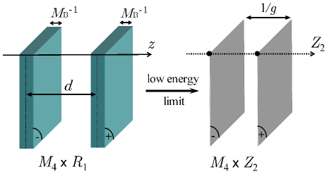
Figure 1: (Color online). Sketch of a two-brane universe in a $M_{4}\times R_{1}$ bulk. Branes are characterized by a thickness $M_{B}^{-1}$ – where $M_{B}$ is the brane energy scale – with respect to an extra dimension $z$ and an interbrane distance $d$. At low energy, the fermion dynamics in this universe is the same as in a $M_{4}\times Z_{2}$ non commutative two-sheeted spacetime where the effective distance $\delta=1/g$ is related to the coupling constant $g$ between the fermion states localized in each brane.

III Neutron-hidden neutron coupling in a $M_{4}\times S_{1}/Z_{2}$ bulk

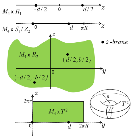
Figure 2: (Color online). Sketches of the extra-dimensional parts of the bulks under consideration for a two-braneworld Universe.

This section pursues the phenomenological investigations, regarding a two-braneworld Universe in a 5-dimensional bulk, introduced in our preliminary work art50 and in which the coupling constant $g$ for a neutron was computed for a $SO(3,1)$-broken 5-dimensional $M_{4}\times R_{1}$ bulk. In this paper, a similar calculation is derived, but now for a 5D $M_{4}\times S_{1}/Z_{2}$ orbifold bulk. The interest of such a scenario arises from the supergravity model of Hořava-Witten art31 . Their approach makes possible the link between the $E_{8}\times E_{8}$ heterotic super-string theory in 10 dimensions and the 11-dimensional supergravity on the orbifold $M_{10}\times S_{1}/Z_{2}$, where 6 of the 11 dimensions are compactified on a Calabi-Yau manifold. At low energy, this model leads then to a $M_{4}\times S_{1}/Z_{2}$ Universe with two 3-branes localized at the boundaries of the $S_{1}/Z_{2}$ orbifold. Such a configuration is considered for instance in ekpyrotic scenarios art60 ; art73 , in the Randall-Sundrum I model art88 , or in the Chung-Freese approach art29 . In these models, a warped metric is often included. Nevertheless, as shown in our previous work art50 , while there is a bare brane energy scale (or bare brane thickness) for a flat metric, the warped metric induces an effective brane energy scale (or effective brane thickness). Experimentally, bare and effective energy scales cannot be distinguish from each other. As a consequence, in the present work, all calculations are made with a Minkowski metric.

The phenomenological model here under consideration, and related calculations, are fully introduced and described elsewhere art50 for a $M_{4}\times R_{1}$ bulk. Nevertheless, the reader will find more details in section IV since they are necessary to explain how to deal with 6-dimensional bulks. As basic hypotheses, one considers fermion sectors $\psi_{+}$ and $\psi_{-}$ respectively which exist only on branes $(+)$ and $(-)$ respectively, and a massless fermion sector $\Psi$ able to propagate through the whole bulk. Each sectors are coupled to each other on each brane through the action art50 :

$$S_{coupling} = -\int d^{4}xdz\sqrt{\left|g^{(4)}\right|}$$

$$\times\left\{\frac{m}{M_{B}^{1/2}}\left(\overline{\psi}_{+}\Psi+\overline{\Psi}\psi_{+}\right)\delta(z-d/2)\right.$$

$$\left.+\frac{m}{M_{B}^{1/2}}\left(\overline{\psi}_{-}\Psi+\overline{\Psi}\psi_{-}\right)\delta(z+d/2)\right\},$$

for two branes located at $z=\pm d/2$ for instance (see Fig. 2). Let us call $G(z|z^{\prime})$ the propagator of the bulk sector $\Psi$ along the extra dimension. The bulk Dirac matrices $\Gamma^{A}$ are such that $\left\{\Gamma^{A},\Gamma^{B}\right\}=2\eta^{AB}\mathbf{1}_{4\times 4}$ ($A,B=0,1,\ldots,4$) with $\eta^{AB}$ the Minkowski metric with a $(+,-,-,-,-)$ signature, and $\Gamma^{4}=-i\gamma_{5}$. Then, it can be proved art50 that the coupling constant $g$ is equal to the component of $2(m^{2}/M_{B})G(d/2|-d/2)$ proportional to $\gamma_{5}$. For instance, Eq. (1) is obtained by considering the bulk sector propagator along the extra dimension $R_{1}$ in a $M_{4}\times R_{1}$ bulk art50 :

$$G(z) = \frac{1}{2\pi}\int\frac{i\gamma^{5}\kappa+m}{\kappa^{2}+m^{2}}e^{-i\kappa z}d\kappa$$ (5)

$$= (1/2)e^{-m\left|z\right|}\left(\mathbf{1}+sign(z)\gamma^{5}\right),$$

For a $M_{4}\times S_{1}/Z_{2}$ bulk, the propagator expression given by Eq. (5) is no longer valid. The $S_{1}/Z_{2}$ symmetry must be taken into account. First, the $G_{S_{1}}(z)$ propagator, along $S_{1}$ only, can be easily obtained from $G(z)$ thanks to a periodic summation with period $2\pi R$ art90 :

$$G_{S_{1}}(z)=\displaystyle\sum_{n=-\infty}^{+\infty}G(z+n\ 2\pi R).$$ (6)

Then, the $G_{S_{1}/Z_{2}}(z)$ propagator can be found thanks to the relationship linking the propagator to the bulk field eigenstates art90 :

$$G_{S_{1}/Z_{2}}(z)=\langle\Psi(z)\bar{\Psi}(z)\rangle,$$ (7)

where $\Psi(z)$ is a linear combination of the two possible solutions induced by a $Z_{2}$ symmetry:

$$\Psi(z)=\frac{1}{2}(\chi(z)+\gamma^{5}\chi(-z)),$$ (8)

with $\chi$ the periodical eigenstate with period $2\pi R$ resulting of the $S_{1}$ symmetry. From Eqs. (7) and (8) it is possible to deduce the $S_{1}/Z_{2}$ propagator from $G_{S_{1}}$, and one obtains:

$$G_{S_{1}/Z_{2}}(z|z^{\prime}) = \frac{1}{4}\Bigg{\{}G_{S_{1}}(z-z^{\prime})-G_{S_{1}}(-z+z^{\prime})$$ (9)

$$-G_{S_{1}}(z+z^{\prime})\gamma^{5}+G_{S_{1}}(-z-z^{\prime})\gamma^{5}\Bigg{\}}.$$

From Eqs. (5), (6) and (9), it results the following expression:

$$G_{S_{1}/Z_{2}}(z|z^{\prime}) = \frac{1}{4}\displaystyle\sum_{n=-\infty}^{+\infty}\Bigg{\{}e^{-m\left|z-z^{\prime}-2\pi Rn\right|}sign(z-z^{\prime}-2\pi Rn)\gamma^{5}$$ (10)

$$-e^{-m\left|z+z^{\prime}-2\pi Rn\right|}sign(z+z^{\prime}-2\pi Rn)\Bigg{\}},$$

with $\Gamma^{0}G^{\dagger}(z)\Gamma^{0}=G(-z)$. Following the same procedure than in our previous paper art50 by using the propagator expressed by Eq. (10), the coupling constant $g$ can be evaluated against the position of the braneworlds on the orbifold $S_{1}/Z_{2}$ (see Fig. 2). When the branes are localized at the orbifold limits, i.e. at $z=0$ and $z=\pi R$, the coupling constant $g$ drops to $0$, meaning that no geometrical coupling is allowed in such a situation. But if one considers our brane located at $z=0$ and the hidden one at $z=d$ (where $d\in\left]0,\pi R\right[$) – i.e. the hidden brane lurks along $S_{1}/Z_{2}$ – the coupling constant between neutron and hidden neutron is now given by:

$$g=\frac{m^{2}}{M_{B}}\left(\frac{e^{md}-e^{-md+m2\pi R}}{1-e^{m2\pi R}}\right),$$ (11)

with $m$ the mass of the quark constituent ($340$ MeV art106 ), $M_{B}$ the brane energy scale and $R$ the compactification radius. For $R\rightarrow+\infty$, we retrieve the non-compactified 5-dimensional case given by expression 1 and for $d\rightarrow\pi R$, we retrieve $g=0$.

IV Neutron-hidden neutron coupling in a flat non-compact 6D bulk

As a beginning and a prerequisite, let us now describe the coupling between two braneworlds in a flat non-compact 6-dimensional bulk. We follow the same approach as previously art50 . This will allow us to consider in section V the coupling between each brane in an ADD-like scenario art78 ; art79 . We consider two 3-branes respectively located at $(y,z)=(d/2,b/2)$ and $(y,z)=(-d/2,-b/2)$ (see Fig. 2). The coupling action $S_{c}$ between the 6D brane sectors $\Psi_{\pm}$ and the 6D bulk sector $\Psi$ is now given by:

$$S_{c} = \int d^{6}x\Bigg{\{}-\frac{m}{M_{B}}(\overline{\Psi}_{+}\Psi+\overline{\Psi}\Psi_{+})\delta(y-d/2)\delta(z-b/2)$$

$$-\frac{m}{M_{B}}(\overline{\Psi}_{-}\Psi+\overline{\Psi}\Psi_{-})\delta(y+d/2)\delta(z+b/2)\Bigg{\}}.$$

The energy scale of the branes $M_{B}$, with $M_{B}^{-1}$ the extradimensional extent of the braneworld in the bulk, is introduced to take into account the extradimensional volume in which the coupling interaction occurs. By contrast with Eq. (III), the power $1$ of $M_{B}$ ensures the correct dimensionality of the problem. The braneworld $S_{\pm}$ action is given by:

$$S_{\pm}=\int d^{4}x\ \overline{\psi}_{\pm}\ (i\gamma^{\mu}\partial_{\mu}+iqA_{\mu}^{\pm}-m)\ \psi_{\pm},$$ (13)

where $\mu=0,1,2,3$ and with $\psi_{\pm}$ the 4D brane sectors and $A^{\pm}$ the electromagnetic vector potentials on each brane. The bulk field $\Psi$ action $S_{bulk}$ is given by:

$$S_{bulk}=\int d^{6}x\ \overline{\Psi}\left(i\Gamma^{A}\left(\partial_{A}+iq\mathcal{A}_{A}\right)\right)\Psi,$$ (14)

where $A=0,1,2,3,5,6$ and $\mathcal{A}_{A}$ is the electromagnetic vector potential of the bulk. It is noteworthy that the electromagnetic potential is assumed to exist only on the braneworlds, with $\mathcal{A}_{4}=\mathcal{A}_{5}=0$ art4 . Here the bulk Dirac matrices $\Gamma^{A}$ are such that $\left\{\Gamma^{A},\Gamma^{B}\right\}=2\eta^{AB}\mathbf{1}_{8\times 8}$ with $\eta^{AB}$ the Minkowski metric with a $(+,-,-,-,-,-)$ signature. We then use the following 8-dimensional Dirac matrices $\Gamma^{A}$:

$$\Gamma^{\mu} = \sigma_{1}\otimes\gamma^{\mu}=\left(\begin{array}[]{cc}0&\gamma^{\mu}\\ \gamma^{\mu}&0\end{array}\right);$$ (17)

$$\text{ }\Gamma^{5} = -i\sigma_{1}\otimes\gamma^{5}=\left(\begin{array}[]{cc}0&-i\gamma^{5}\\ -i\gamma^{5}&0\end{array}\right);\text{ }$$ (20)

$$\Gamma^{6} = -i\sigma_{2}\otimes\mathbf{1}_{4\times 4}=\left(\begin{array}[]{cc}0&-\mathbf{1}_{4\times 4}\\ \mathbf{1}_{4\times 4}&0\end{array}\right),$$ (23)

and such that the chiral matrice $\Gamma^{7}=-\Gamma^{0}\Gamma^{1}\Gamma^{2}\Gamma^{3}\Gamma^{5}\Gamma^{6}$ is given by:

$$\Gamma^{7}=\sigma_{3}\otimes\mathbf{1}_{4\times 4}=\left(\begin{array}[]{cc}\mathbf{1}_{4\times 4}&0\\ 0&-\mathbf{1}_{4\times 4}\end{array}\right).$$ (24)

The chiral 6D states are then defined through:

$$\left(\frac{1\pm\Gamma^{7}}{2}\right)\Psi=\Psi_{R/L},$$ (25)

and $\Psi$ can be written as:

$$\Psi=\left(\begin{array}[]{c}\psi_{R}\\ \psi_{L}\end{array}\right)\mathrm{such\ that}\ \Psi_{R}=\left(\begin{array}[]{c}\psi_{R}\\ 0\end{array}\right)\mathrm{and}\ \Psi_{L}=\left(\begin{array}[]{c}0\\ \psi_{L}\end{array}\right)\mathrm{.}$$ (26)

Now, regarding the 6D brane sectors $\Psi_{\pm}$, the 6D chiral states do not correspond to the 4-dimensional ones on the branes. Indeed, the 6D chirality appears as an extra quantum number added to the usual particles of the Standard Model on a brane, thus doubling the Standard Model on the brane, a situation which is not observed. As a consequence, we assume that each brane can only support one 6D chiral state, for instance the left one, while the other cannot be trapped on the brane. Such a situation is supported by the works dealing with the domain wall description of branes where it is known that the fermions’ trapping on branes depends on their chirality art26 ; art91 ; art92 ; art93 ; art94 ; art95 ; art96 ; art97 ; art98 ; art99 ; art100 ; art101 ; art4 ; art102 ; art103 . As an ansatz, the brane sectors are given by:

$$\Psi_{\pm}=\left(\begin{array}[]{c}0\\ \psi_{\pm}\end{array}\right),$$ (27)

and where $\psi_{\pm}$ follow the action given by Eq. (13) thanks to the above choice for the gamma matrices and in accordance with the 6D action in Eq. (14).

Now, from the whole action, the bulk field follows:

$$\left(i\Gamma^{A}\left(\partial_{A}+iq\mathcal{A}_{A}\right)\right)\Psi=\frac{m}{M_{B}}\Psi_{+}\delta(y-d/2)\delta(z-b/2)+\frac{m}{M_{B}}\Psi_{-}\delta(y+d/2)\delta(z+b/2),$$ (28)

where the fields on each braneworld act as sources (or wells) for the bulk field.

From Eq. (28) and using the mass shell condition art50 $\left(i\Gamma_{\pm}^{\mu}\left(\partial_{\mu}+iqA_{\mu}\right)-m\right)\Psi=0$, one deduces the following propagator for the bulk sector along extra dimensions:

$$G(y,z) = \frac{1}{4\pi^{2}}\int\int\frac{\Gamma^{5}q+\Gamma^{6}\kappa+m}{q^{2}+\kappa^{2}+m^{2}}e^{i\kappa z}e^{iqy}d\kappa dq$$

$$= \frac{1}{2\pi}\frac{im}{\sqrt{z^{2}+y^{2}}}K_{1}(m\sqrt{z^{2}+y^{2}})\left(sign(y)\ |y|\ \Gamma^{5}+sign(z)\ |z|\ \Gamma^{6}\right)$$

$$+\frac{m}{2\pi}K_{0}(m\sqrt{z^{2}+y^{2}}),$$

with $\Gamma^{0}G^{\dagger}(y,z)\Gamma^{0}=G(-y,-z)$ and from which $\Psi$ can be expressed thanks to Eq. (28):

$$\Psi(x,y,z)=\frac{m}{M_{B}}G(y-d/2,z-b/2)\Psi_{+}(x)+\frac{m}{M_{B}}G(y+d/2,z+b/2)\Psi_{-}(x).$$ (30)

Injecting Eq. (30) in the coupling action given by Eq. (IV) and looking for the $M_{4}\times Z_{2}$ effective action $S_{M_{4}\times Z_{2}}=S_{+}+S_{-}+S_{c}$ given by Eqs. (2) and (3), one successively gets:

$$S_{c}=-\frac{2m^{2}}{M_{B}^{2}}\int d^{4}x\Bigg{\{}\overline{\Psi}_{+}G(d,b)\Psi_{-}+\overline{\Psi}_{-}G(-d,-b)\Psi_{+}\Bigg{\}}$$ (31)

and

$$S_{M_{4}\times Z_{2}} = \int d^{4}x\ \Bigg{\{}\overline{\psi}_{+}\ (i\gamma^{\mu}\partial_{\mu}+iqA_{\mu}^{+}-m)\ \psi_{+}$$

$$+\overline{\psi}_{-}\ (i\gamma^{\mu}\partial_{\mu}+iqA_{\mu}^{-}-m)\ \psi_{-}$$

$$+ig\overline{\psi}_{+}\gamma^{5}\psi_{-}+ig\overline{\psi}_{-}\gamma^{5}\psi_{+}$$

$$-im_{r}\overline{\psi}_{+}\psi_{-}+im_{r}\overline{\psi}_{-}\psi_{+}\Bigg{\}},$$

with the coupling constant $g$ given by:

$$g=\frac{m^{3}}{\pi M_{B}^{2}}\frac{d}{D}K_{1}(mD),$$ (33)

and

$$m_{r}=\frac{m^{3}}{\pi M_{B}^{2}}\frac{b}{D}K_{1}(mD),$$ (34)

where $D$ is the distance between the two braneworlds (see Fig. 2), with $D=\sqrt{d^{2}+b^{2}}$ and $m$ the mass of a constituent quark ($340$ MeV) when considering the neutron-hidden neutron coupling art106 ; art50 . It is interesting to note that due to the bulk symmetry breaking induced by the branes regarding to the 6D chirality, $g$ or $m_{r}$ can vanishe depending on the value of $d$ or $b$. For instance, if $b=0$, $m_{r}$ is now equal to zero, and Eq. (33) reduces to:

$$g=\frac{m^{3}}{\pi M_{B}^{2}}K_{1}(md).$$ (35)

V Neutron-hidden neutron coupling in an ADD bulk

The last case introduced in this paper is the compactification of the two extra dimensions on a torus ($T^{2}\equiv S_{1}\times S_{1}$ manifold), with two 3-branes respectively located at $(y,z)=(0,0)$ and $(y,z)=(d,0)$, with $d\in\ ]0,2\pi R[$ (see Fig. 2). This model is of interest as it is reminiscent of the ADD scenario art78 ; art79 but with two branes. Using the same approach as in section III to derive the propagator in a compactified bulk, the propagator for the bulk sector on the torus can be deduced from Eq. (IV), and we get:

$$G(y,z)=\displaystyle\sum_{n=-\infty}^{+\infty}\displaystyle\sum_{k=-\infty}^{+\infty}\Big{\{}\frac{1}{2\pi}\frac{imK_{1}(m\sqrt{(y+n2\pi R)^{2}+(z+k2\pi r)^{2}})}{\sqrt{(y+n2\pi R)^{2}+(z+k2\pi r)^{2}}}$$ (36)

$$\times\left(sign(y+n2\pi R)\ |y+n2\pi R|\ \Gamma^{5}+sign(z+k2\pi r)\ |z+k2\pi r|\ \Gamma^{6}\right)$$

$$+\frac{m}{2\pi}K_{0}(m\sqrt{(y+n2\pi R)^{2}+(z+k2\pi r)^{2}})\Big{\}},$$

with $r$ and $R$ the compactification radii of the extra dimensions (see Fig. 2). It leads to the following coupling constant $g$ expression:

$$g = \frac{m^{3}}{\pi M_{B}^{2}}\displaystyle\sum_{n=-\infty}^{+\infty}\displaystyle\sum_{k=-\infty}^{+\infty}\frac{K_{1}(m\sqrt{(d+n2\pi R)^{2}+(k2\pi r)^{2}})}{\sqrt{(d+n2\pi R)^{2}+(k2\pi r)^{2}}}$$

$$\times sign(d+n2\pi R)\ |d+n2\pi R|\$$

for which there is no trivial expression. It is notheworthy that, as for the compact 5-dimensional case introduced in section III, some locations ($d=\pi R$ for instance) of the braneworlds cancel the coupling. When $r,R\rightarrow+\infty$, i.e. the torus tends towards a plane, all terms in the summation in Eq. (V) tend towards zero, except for $(n,k)=(0,0)$, thus leading to the expected expression Eq. (35).

VI Discussion

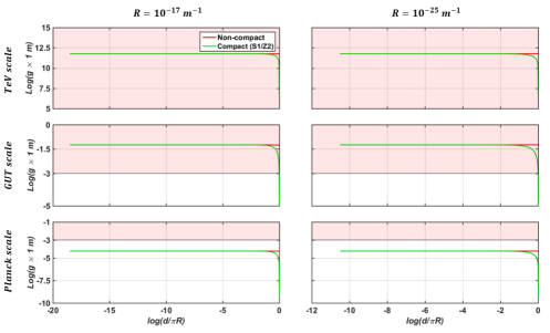
Figure 3: (Color online). Neutron-hidden neutron coupling constant $g$ against interbrane distance $d\in\ ]0,\pi R[$ for a 5-dimensional bulk with 1 extra dimension compactified on a $S_{1}/Z_{2}$ orbifold. $g$ is plotted for three braneworld energy scales (the TeV scale, the GUT scale and the Planck scale) and for two compactification radii ($R$) chosen arbitrarily ($R=10^{-17}$ m^-1 and $R=10^{-25}$ m^-1). Red curves represent the non-compact 5-dimensional case and green curves the $S_{1}/Z_{2}$ compact case. Red regions for values greater than $g=200$ peV (or $10^{-3}$ m^-1 in natural units) are excluded with confidence from experimental data art6 . For interbrane distances greater than $0.5$ fm, neutron exchange is supposed to be precluded ($g=0$ m^-1) by the model art50 .

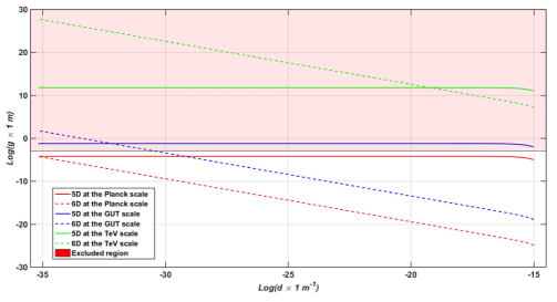
Figure 4: (Color online). Neutron-hidden neutron coupling constant $g$ against interbrane distance $d$ for non-compact 5-dimensional and 6-dimensional bulks and for various brane energy scales $M_{B}$, i.e the TeV scale, the GUT scale and the Planck scale. Solid lines represent the 5-dimensional bulk and dash curves the 6-dimensional bulk. Red regions for values greater than $g=200$ peV (or $10^{-3}$ m^-1 in natural units) are ruled out from stringent experimental data art6 . For interbrane distances greater than $0.5$ fm, neutron exchange is supposed to be precluded ($g=0$ m^-1) by the model art50 .

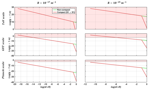
Figure 5: (Color online). Neutron-hidden neutron coupling constant $g$ against interbrane distance $d\in\ ]0,\pi R[$ for a 6-dimensional bulk with 2 extra dimensions compactified on a $S_{1}\times S_{1}$ manifold, i.e. a torus. $g$ is plotted for three braneworld energy scales (the TeV scale, the GUT scale and the Planck scale) and for two compactification radii ($r$ and $R$) chosen arbitrarily ($R=r=10^{-17}$ m^-1 and $R=r=10^{-25}$ m^-1). Red regions for values greater than $g=200$ peV (or $10^{-3}$ m^-1 in natural units) are excluded with confidence from experimental data art6 . For interbrane distances greater than $0.5$ fm, neutron exchange is supposed to be precluded ($g=0$ m^-1) by the model art50 .

The disappearance of a geometrical coupling for two braneworlds located at the $S_{1}/Z_{2}$ orbifold limits makes impossible to constrain the Hořava-Witten 11-dimensional supergravity art31 with neutron-hidden neutron transitions. However, for any other locations of the branes, the expression of the coupling constant is given by Eq. (11). Such locations are allowed in the context of some ekpyrotic scenarios art60 ; art73 . Figure 3 shows the behavior of the neutron coupling constant against the interbrane distance $d$ for an extra dimension compactified on a $S_{1}/Z_{2}$ orbifold (green points derived from Eq. (11), compared to the non-compact case art50 (red line). In Fig. 3, $g$ is plotted for two compactification radii (chosen arbitrarily), i.e $R=10^{-17}$ m^-1 and $R=10^{-25}$ m^-1, and for three brane energy scales: the TeV scale, the GUT scale and the Planck scale. For the TeV scale, the $S_{1}/Z_{2}$ compact case is ruled out as well as the non-compact case. For the GUT scale, the drop of the coupling for the compact case makes impossible to exclude this scenario for interbrane distances $d\rightarrow\pi R$. For the Planck energy scale, the non-compact case is very close to be excluded with future passing-through-walls neutron experiments art6 ; art24 while significant improvements are needed to rule out the compact case for interbrane distances close to $\pi R$ .

Figure 4 shows the neutron-hidden neutron coupling constant $g$ in function of the interbrane distance in a non-compact bulk for one extra dimension (from Eq. (1)) and for two extra dimensions (from Eq. (35)). Here again, three braneworld energy scales $M_{B}$ are also considered: the TeV scale, the GUT scale and the Planck scale. Braneworlds related to the TeV energy scale are fully excluded for one as well as for two extra dimensions. Braneworlds related to the GUT energy scale are also ruled out for one extra dimension. As shown in Fig. 4, the transition from a 5-dimensional bulk to a 6-dimensional one significantly reduces the coupling constant values for GUT and Planck scales. While the Planck scale for one non-compact extra dimension is almost reachable by experiments art6 , the 6-dimensional case is far beyond the sensitivity of passing-through-walls neutron experiments art6 . The present results show the impossibility for current passing-through-walls neutron experiments to constrain all the range of interbrane distances for GUT and Planck scales for bulks with more than 5 dimensions. Indeed, the swapping probability $p$ (see sections I and II) and the coupling constant $g$ are related as $g=\sqrt{p}$. While a gain of a factor $10$ on the last constrain found in 2016 ($p<4.6\times 10^{-10}$ at 95% CL) is expected for future passing-through-walls neutron experiments, the 6-dimensional case is far to be reachable by such experiments.

Finally, Fig. 5 shows the coupling constant $g$ against the interbrane distance $d$ for two extra dimensions compactified on a $S_{1}\times S_{1}$ manifold, i.e. a torus. As previously, we explore the same three energy scales (TeV, GUT and Planck scales). Two compactification radii are chosen (arbitrarily): $R=r=10^{-17}$ m^-1 and $R=r=10^{-25}$ m^-1. As shown by Fig. 5, the compactification leads to a decrease of the coupling for interbrane distances $d\rightarrow\pi R$ with respect to the non-compact case. While the TeV energy scale is completely ruled out whatever the values of compactification radii, all the parameter range of GUT and Planck scales are unreachable for the sensitivity of current and future passing-through-walls neutron experiments.

VII Conclusions

Many scenarios consider hidden braneworlds in the vicinity of our visible one, living together in a N-dimensional bulk. Here we have described the behavior of the neutron-hidden neutron coupling constant – an experimentally measurable parameter – for various bulks. It has been first shown that the Hořava-Witten 11-dimensional supergravity and related models cannot be excluded with passing-through-walls neutron experiments. But it is not the case for some ekpyrotic scenarios provided that one braneworld, at least, is not located on a boundary of the $M_{4}\times S_{1}/Z_{2}$ orbifold. Next, we have considered 6D bulks, with two extralarge extra dimensions or compactified on a torus in an ADD-like configuration. The addition of more than one extra dimension significantly drops the coupling constant values, making possible yet to test these scenarios but precluding to fully rule out the whole range of braneworld models. While braneworlds endowed with their own copy of the Standard Model at a TeV energy scale are already experimentally excluded, those at GUT or Planck scale are still reachable and their existence could be either confirmed or rejected for 5D bulks. By contrast, future experiments involving neutron disappearance-reappearance could constrain 6D bulks scenarios but cannot totally exclude them. Such a situation prevents to definitively close these lines of theoretical research.

References

- [1] A. Dobado J. A. R. Cembranos and A. L. Mardo. Brane-world dark matter. Phys. Rev. Lett. 90 (2001) 241301.
- [2] Ph. Brax, C. Van de Bruck and A.C. Davis. Brane world cosmology. Rep. Prog. Phys. 67 (2004) 12.
- [3] J-L Lehners. Ekpyrotic and cyclic cosmology. Phys. Rept. 465 (2008) 223-263.
- [4] R. Maartens and K. Koyama. Brane-world gravity. Living Rev. Relativity 13 (2010) 5.
- [5] M. A. Garcìa-Aspeitia, J. Magaña and T. Matos. Braneworld model of dark matter: structure formation. Gen. Relativ. Gravit. 44 (2012) 581-601.
- [6] T. Koivistoa, D. Wills and I. Zavalae. Dark D-brane cosmology. J. Cosmol. Astropart. Phys. 2014 (2014).
- [7] D. Battefeld and P. Peters. A critical review of classical bouncing cosmologies. Phys. Rept. 571 (2015) 1-66.
- [8] C. Van De Bruck and E. M. Teixeira. Dark D-brane cosmology: from background evolution to cosmological perturbations. arXiv:2007.15414.
- [9] F. Petit and M. Sarrazin. Quantum dynamics of massive particles in a non-commutative two-sheeted space-time. Phys. Lett. B 612 (2005) 105-114.
- [10] M. Sarrazin and F. Petit. Matter localization and resonant deconfinement in a two-sheeted spacetime. Int. J. Mod. Phys. A 22 (2007) 2629-2642.
- [11] M. Sarrazin and F. Petit. Equivalence between domain-walls and ”noncommutative” two-sheeted spacetimes: Model-independent matter swapping between branes. Phys. Rev. D 81 (2010) 035014.
- [12] M. sarrazin and F. Petit. Brane matter, hidden or mirror matter, their various avatars and mixings: many faces of the same physics. EPJC 72, 2230 (2012).
- [13] C. Stasser and M. Sarrazin. Sub-GeV-scale signatures of hidden braneworlds up to the planck scale in a SO(3, 1)-broken bulk. Int. J. of Phys. Mod. A 34(05):1950029 (2019).
- [14] M. Sarrazin and F. Petit. Laser frequency combs and ultracold neutrons to probe braneworlds through induced matter swapping between branes. Phys. Rev. D 83 (2011) 035009.
- [15] M. Sarrazin, G. Pignol, F. Petit and V.V. Nesvizhevsky. Experimental limits on neutron disappearance into another braneworld. Phys. Lett. B 712 (2012) 213.
- [16] M. Sarrazin, G. Pignol, J. Lamblin, F. Petit, G. Terwagne, V. V. Nesvizhevsky. Probing the braneworld hypothesis with a neutron-shining-through-a-wall experiment. Phys. Rev. D 91, 075013 (2015).
- [17] M. Sarrazin, G. Pignol, J. Lamblin, J. Pinon, O. Méplan, G. Terwagne, P-L. Debarsy, F. Petit, V. V. Nesvizhevsky. Search for passing-through-walls neutrons constrains hidden braneworlds. Phys. Lett. B 758 (2016) 14.
- [18] C. Stasser, M. Sarrazin and G. Terwagne. Search for neutron-hidden neutron interbrane transitions with murmur, a low-noise neutron passing-through-walls experiment. EPJ Web of Conferences, 2019.
- [19] G. Dvali, G. Gabadadze and M. Porrati. 4D gravity on a brane in 5D minkowski space. Phys. Lett. B 485 (2000) 208-214.
- [20] G. Dvali, G. Gabadadze and M. Shifman. (quasi)localized gauge field on a brane: Dissipating cosmic radiation to extra dimensions? Phys. Lett. B 497 (2001) 271.
- [21] D.J.H. Chung and K. Freese. Can geodesics in extra dimensions solve the cosmological horizon problem? Phys. Rev. D 62 (2000) 063513.
- [22] D.J.H. Chung, E. W. Kolb and A. Riotto. Extra dimensions present a new flatness problem. Phys. Rev. D 65 (2002) 083516.
- [23] D.J.H. Chung and K. Freese. Lensed density perturbations in braneworlds: An alternative to perturbations from inflation. Phys. Rev. D 67 (2003) 103505.
- [24] D. Griths. Introduction to elementary particles. Wiley-VCH Verlag GmbH & Co., 2008.
- [25] P. Horava and E. Witten. Heterotic and type I string dynamics from eleven dimensions. Nucl. Phys. B 460 (1996) 506.
- [26] N. Arkani-Hamed, S. Dimopoulos and G. Dvali. The hierarchy problem and new dimensions at a millimeter. Phys. Lett. B 429 (1998) 263-272.
- [27] N. Arkani-Hamed, S. Dimopoulos and G. Dvali. Phenomenology, astrophysics and cosmology of theories with sub-millimeter dimensions and TeV scale quantum gravity. Phys. Rev. D 59 (1999) 086004.
- [28] J. Khoury, B.A. Ovrut, P.J. Steinhardt and N. Turok. Ekpyrotic universe: colliding branes and the origin of the hot big bang. Phys. Rev. D64 (2001) 123522.
- [29] G. W. Gibbons, H. Lü and C. N. Pope. Brane worlds in collision. Phys. Rev. Lett. 94 (2005) 131602.
- [30] L. Randall and R. Sundrum. Large mass hierarchy from a small extra dimension. Phys. Rev. Lett. 83 (1999) 3370.
- [31] H. Georgi, A. K. Grant and G. Hailu. Brane couplings from bulk loops. Phys. Lett. B 506 (2001) 207-214.
- [32] V.A. Rubakov and M.E. Shaposhnikov. Do we live in a domain wall? Phys. Lett. 125B (1983) 136.
- [33] N. Arkani-Hamed and M. Schmaltz. Hierarchies without symmetries from extra dimensions. Phys. Rev. D 61 (2000) 033005.
- [34] S. Randjbar-Daemi and M. Shaposhnikov. On some new warped brane world solutions in higher dimensions. Phys. Lett. B 492 (2000) 361.
- [35] L. Dubovsky, V. A. Rubakov and P. G. Tinyakov. Brane world: disappearing massive matter. Phys. Rev. D 62 (2000) 10501.
- [36] A. Kehagias and K. Tamvakis. Localized gravitons, gauge bosons and chiral fermions in smooth spaces generated by a bounce. Phys. Lett. B 504 (2001) 38.
- [37] B. Bajc and G. Gabadadze. Localization of matter and cosmological constant on a brane in anti de sitter space. Phys. Lett. B 474 (2000) 282.
- [38] C. Ringeval, P. Peter and J. P. Uzan. Localization of massive fermions on the brane. Phys. Rev. D 65 (2002) 044016.
- [39] R. Koley and S. Kar. Scalar kinks and fermion localisation in warped spacetimes. Class. Quant. Grav. 22 (2005) 753.
- [40] A. Melfo, N. Pantoja and J. D. Tempo. Fermion localization on thick branes. Phys. Rev. D 73 (2006) 044033.
- [41] R. Guerrero, A. Melfo, N. Pantoja and R. O. Rodriguez. Self-gravitating non-abelian kinks as brane worlds. Phys. Rev. D 74 (2006) 084025.
- [42] Y. X. Liu, Z. H. Zhao, S. W. Wei and Y. S. Duan. Bulk matters on symmetric and asymmetric de sitter thick branes. JCAP 0902 (2009) 003.
- [43] Y. X. Liu, J. Yang, Z. H. Zhao, C. E. Fu and Y. S. Duan. Fermion localization and resonances on a de sitter thick brane. Phys. Rev. D 80 (2009) 065019.
- [44] D. Bazeia, A. Mohammadi and D. C. Moreira. Fermion bound states in geometrically deformed backgrounds. Chin. Phys. C 43 (2019) 013101.
- [45] R. Guerrero, R.O. Rodriguez and F. Carreras. Fermion bound states in geometrically deformed backgroundmassless fermions localization on domain walls. Revista Mexicana de Fisica 66 (2020) 77–81.