GEFA: Early Fusion Approach in Drug-Target Affinity Prediction

Abstract

Predicting the interaction between a compound and a target is crucial for rapid drug repurposing. Deep learning has been successfully applied in drug-target affinity (DTA) problem. However, previous deep learning-based methods ignore modeling the direct interactions between drug and protein residues. This would lead to inaccurate learning of target representation which may change due to the drug binding effects. In addition, previous DTA methods learn protein representation solely based on a small number of protein sequences in DTA datasets while neglecting the use of proteins outside of the DTA datasets. We propose GEFA (Graph Early Fusion Affinity), a novel graph-in-graph neural network with attention mechanism to address the changes in target representation because of the binding effects. Specifically, a drug is modeled as a graph of atoms, which then serves as a node in a larger graph of residues-drug complex. The resulting model is an expressive deep nested graph neural network. We also use pre-trained protein representation powered by the recent effort of learning contextualized protein representation. The experiments are conducted under different settings to evaluate scenarios such as novel drugs or targets. The results demonstrate the effectiveness of the pre-trained protein embedding and the advantages our GEFA in modeling the nested graph for drug-target interaction.

1 Introduction

Predicting drug-target binding affinity (DTA prediction) is crucial in new drug development as well as drug repurposing [1]. The gold standard to determine the binding affinity is by experimental assays but this is prohibitively expensive as a rapid screening tool as there are over 100 million drug-like compounds [2] and over 5000 potential protein targets [3]. Therefore, it is necessary to have alternative computational methods using simulation or machine learning to predict the binding affinity of novel drug-target pairs. Machine learning methods are particularly attractive because they offer cheap and fast alternatives with reasonable performance thanks to the large DTA databases [3] that we can leverage on.

With the advance of machine learning, many computational prediction methods [4, 5, 6, 7] have been proposed to tackling DTA. In recent works, the protein is typically represented as a string of amino acids denoted by letters [6, 7, 8]. The drawback of using protein sequence is that it can not represent the 3D structure of the protein which is crucial information for determining the binding affinity between protein and drug in practice[9]. However, obtaining the high-resolution 3D structure is a challenging task. A more practical solution is using the 2D residue contact maps to represent tertiary protein structure. These maps can now be determined with reasonable accuracy from deep learning powered algorithms [10, 11].

The contact map can be naturally modeled using recent advances in deep learning known as graph neural networks (GNN). Here each residue is represented as a node in the graph, and a contact between two residues as an edge. Each node is first embedded with a feature vector. The GNN operates by iteratively sending messages between nodes, effectively refining the node representation by collecting information from its neighbors and distant nodes. Then the protein representation can be pooled from its residues.

Previous deep learning-based DTA prediction methods [6, 7, 8, 12] often use the late fusion approach. The late fusion approach extracts drug and target representation separately then predicts the binding affinity from the combined representation at the very end of the process. However, this practice ignores the fact that the binding occurs at a pocket rather than the whole protein. The pocket is a small convex cave in the 3D structure of the protein that encourages stable binding of a drug to the protein. Once the drug binds, it changes the protein functions to have pharmaceutical effects, hence it can also change the protein structure [13], hence its representation. As the late fusion approach only combines drug and target representation extracted from the input, the change in protein representation due to the binding process is not addressed. In addition, the model assumes non site-specific binding, making it difficult to assign the credit to the sites that interact. It can also result in slower learning rate, and less interpretable prediction.

To address target protein representation change, we propose an early-fusion-based approach. Initially, we extract representation feature for a given drug molecule from its drug graph structure. Then, the drug representation is integrated into the protein graph structure before the protein representation learning phrase. This is basically a graph structure nested inside another graph structure. This graph-in-graph neural network design allows the model to learn changes in protein representation caused by the binding process with the drug molecule.

Previous works [8, 6, 7, 14] normally use one-hot encoding to vectorize residues. This conventional approach fails to embed the contextual dependencies between residues as well as not being able to make use of unlabeled protein sequences. Recent advances in natural language processing allow to learn contextual embedding from massive unlabeled data which are the current state-of-the-art on many tasks [15]. Therefore, we take advantage of the power of the protein embedding features learned by a protein language modeling on a large collection of protein sequences, including proteins that are not available in DTA datasets, to represent the residues in a given target protein. In this work, we refer target proteins whose the binding affinities available in the DTA datasets as labeled ones while proteins that do not exist in the DTA datasets as unlabeled proteins.

In summary, the contribution of our work is two-fold. First, we combine the protein sequence embedding feature and protein contact map to build the graph representation of a target protein. Second, in order to reflect the target representation change during the binding process, we propose a so-called Graph Early Fusion for binding Affinity prediction (GEFA) for more accurate biological modeling. We demonstrate the effects of the GEFA on Davis dataset [16] where it has shown superior performance against previous studies on different settings. Our Python implementation and data are publicly available at https://github.com/ngminhtri0394/GEFA.

2 Related Works

2.1 Drug Re-purposing as an Alternative Medication for Novel Disease

Drug re-purposing [17] is the process of identifying well-established medications for the novel target disease. The advantages of this drug re-purposing over developing a completely novel drug are lower risk and fast-track development [18]. The process of drug re-purposing consists of three key steps: identifying the candidate molecules given the target disease, drug effect assessment in the preclinical trial, and effectiveness assessment in clinical trial [19]. The first step, hypothesis generation, is critical as it decides the success of the whole process. Advanced computational approaches are used for hypothesis generation. Computational approaches in drug re-purposing can be categorized into six groups [19]: genetic association [20, 21], pathway pathing [22, 23, 24], retrospective clinical analysis [25, 26, 27], novel data sources, signature matching [28, 29, 30], molecular docking [31, 32, 33].

2.2 Drug-Target Binding Affinity Prediction Problem

Drug-target binding affinity indicates the strength of the binding force between the target protein and its ligand (drug or inhibitor) [34]. The drug-target binding affinity prediction problem is a regression task predicting the value of the binding force. The binding strength is measured by the equilibrium dissociation constant ($K_{D}$). A smaller $K_{D}$ value indicates a stronger binding affinity between protein and ligand [34]. There are two main approaches: structural approach and non-structural approach [1]. Structural methods utilize the 3D structure of protein and ligands to run the interaction simulation between protein and ligand. On the other hand, the non-structural approach relies on ligand and protein features such as sequence, hydrophobic, similarity or other alternative structural information.

2.2.1 Structural Approach

The structure-based approach involves molecular docking, predicting the three-dimensional structure of the target-ligand complex. In molecular docking, there are a large number of target-ligand complex conformations. The conformations are evaluated by the scoring function. Based on the scoring function types, the structural approach can be categories into three groups [1]: classical scoring function method [35, 36, 37, 38], machine learning scoring function method [39], and deep learning scoring function method [40, 41].

2.3 Non-structural Approach

The non-structural approach solves the binding affinity regression task without the accurate 3D structure of the target. Instead of using the 3D coordinate of target and drug atom. The non-structural approach relies on the drug-drug, target-target similarity, target and drug atom sequence, and other alternative structural information such as contact map or secondary structure.

2.3.1 Representation of Protein in Non-structural Approach

The simplest way to represent a protein chain is by a string of letters. Twenty alphabet characters are used to encode twenty types of amino acids. The torsion angle of each amino acid in the protein sequence is represented as a pair of $\phi$ and $\psi$ angle. Amino acids in protein sequence have one of three main types of secondary structure: $\alpha$ helix, $\beta$ pleated sheet, and coil. Therefore, three alphabet characters are used to encode the secondary structure. The interaction between two non-adjacency residues is represented as the contact map or distance map. Two non-adjacency residues are in contact if their distance is less than 8 ${\AA}$. The contact map is the binary map showing whether two residues in the protein chain are in contact.

2.3.2 Kernel Based Approach (KronRLS)

KronRLS [4, 5] uses the kernel-based approach to construct the similarity between drugs or between target proteins. In KronRLS, a kernel is a function measuring the similarity between two molecules. The regularized least squares regression (RLS) framework is used to predict the binding affinity values.

2.3.3 Similarity Matching Approach (SimBoost)

SimBoost [42] constructs features for each drug, target, and drug-target pair from the similarity among drugs and targets. Then similarity-based features are used as input in a gradient boosting machine to predict the continuous value of binding affinity of the drug-target couples.

2.3.4 Deep Learning Based Methods

DeepDTA [6] predicts the binding affinity from the 1D representation of protein and drug. WideDTA [8] is an extension of DeepDTA. Protein is represented not only in sequence but also in motif and domain. The drug is represented in SMILES and Ligand Maximum Common Substructures. The method’s drawback is using sequence to represent drugs and targets. However, the structural information of the drug and the target plays important roles in the drug-target interaction. Instead of using 1D representation for drug, GraphDTA [7] uses graph to express the interaction between atoms of the molecules. This allows modeling the interaction between any two atoms within the drug molecules. However, the protein is still represented as sequence which limits the model performance. PADME [43] uses graph structure to represent the compound and Protein Sequence Information (PSC descriptors) to represent the target. The PSC descriptors contains richer information than the sequence. However, the model performance may be limited without the structural information. DrugVQA [12] uses distance map to represent the protein. Sequential self-attention is used to learn which parts of the protein interact with the ligand. Multi-head self-attention is used to learn which atoms in drugs have high contribution to the drug-target interaction. However, DrugVQA is a supervised learning method without any pretraining on targets or drugs. Therefore, it may not cope well with a novel drug or protein. Graph-CNN [44] pretrains the protein pocket graph autoencoder by minimizing representation difference. The binding interaction model has protein pocket graph and 2D molecular graph as the inputs. The unsupervised learning helps the model to overcome the limited pocket graph training data. However, Graph-CNN requires the protein pockets as target representation which may limit its general usage. DGraphDTA [14] uses contact map to build protein graph structure with PSSM, one-hot encoding, and residue properties as node features. This allows the model to obtain an accurate protein representation. However, DGraphDTA ignores the representation change of the target caused by conformation change. As a result, the target representation learned by the model may be inaccurate.

3 Proposed Methods

The task of drug-target binding affinity (DTA) problem is to predict the binding affinity A between a target protein P and drug compound D. Mathematically, the problem is formulated as a regression task:

$$A=\mathcal{F}_{\theta}(P,D),$$ (1)

where $\theta$ is model parameters of predicting function $\mathcal{F}$.

In this section, we present details of our approach to solve DTA. In Sec. 3.1 explains the feature representation of target protein P, followed by the feature representation of drug compound D in Sec. 3.2. The main contribution of ours is presented in Sec. 3.3 where we aim at reflecting the changes in the target protein representation due to the conformation change.

3.1 Graph Representation of Protein

Previous methods applying deep learning to DTA [6, 8, 7] use target protein sequence whose residues are embedded into vector space, often with one-hot encoding. Subsequently, an encoder of multiple 1D convolution layers are used to obtain a final presentation of the protein sequence. This approach only makes use of the primary structure information of the target protein sequence. However, the tertiary information is important for the drug-target interaction [9]. Even though the 3D representation can precisely describe the tertiary structure, obtaining 3D geometrical structure information of the protein is time-consuming and challenging. This is even impossible for some protein types using NMR or X-ray crystallography [45]. To balance the complexity against efficiency, we utilize the 2D contact map information as the representation of the tertiary structure to represent the protein graph structure.

Given that we have the 2D tertiary structure information, each target protein is considered as a graph structure where nodes are residues in the protein sequence. Previous studies [7, 6] use one-hot encoding to vectorize each residue in a protein sequence. While using one-hot encoding is convenient, it does not tell the similarity between elements but consider them equidistant from each other. In addition, this choice of representation limits the learning capability as it fails to leverage the contextual dependencies between residues, which can be estimated through unsupervised learning. In effect, the learning signals only come from the limited number of target proteins in a particular dataset. In fact, there are only 7605 target proteins [3] being used for the task of drug-target binding affinity (DTA) prediction while the majority of proteins are not being used. It has been estimated that there exist over 188 million sequences of unlabeled target protein sequences[46].

Leveraging this rich set of unlabeled proteins, we utilize state of the art language modeling methods to learn contextual residue embedding representation. We use embedded representation learnt from a large collection of unlabeled protein sequences provided by TAPE [47] instead of one-hot encoding to represent each node in the protein graph. To be more specific, it relies on the latest advance of self-supervised learning which is widely studied in natural language processing. Self-supervised learning is a subset of unsupervised learning where the supervision is derived from the data itself [48]. Generally, a part of data is withheld and the model is trained to predict it. Language modeling is a common case of self-supervised learning in natural language processing in which it learns the representation of sequence using pretext tasks such as predicting missing token or the next token in sequence [15]. TAPE is a variant of language model for protein representation in particular. Subsequently, given a protein sequence of $L$ residues, the node features of the protein graph is a set $\mathcal{V}_{p}=\left\{v_{i}\mid v_{i}\in R{}^{h}\right\}_{i=1}^{L}$, where $h$ is the length of the embedding vector $v_{i}$ provided by TAPE. Each $v_{i}$ is contextual, that is residues occur in the context of surrounding residues. Therefore, the structural information is implicitly encoded into the embedding.

We use secondary structure as it decides the backbone shape of the target protein which also contributes to the shape of the binding site and overall structure. For each residue, the secondary structure feature is represented as the probability of three secondary structure type $\alpha$ helix, $\beta$ pleated sheet, and coil.

Solvent accessibility indicates the level of interaction between residues and drug molecule. Solvent accessibility is divided into three classes: buried (pACC from 0 to 10), medium (pACC from 11 to 40), and exposed (pACC from 41 to 100). Residues buried inside the protein core are less likely to interact with the drug molecule while exposed residues are more likely to interact with drug molecule. Eventually, the combination of embedding vector extracted by TAPE, secondary structure feature vector, and solvent accessibility feature vector are used to represent node features of residues in a target protein graph.

The contact map information provides the contacts between any two residue nodes in a protein graph. The sequence information is also retained in the graph structure in form of edges linking any two nodes of adjacency residues in the protein sequence. In practice, the contact map and sequence information are stored as an adjacency matrix $\mathcal{A}_{p}$. In the rest of this paper, we denote the protein graph as $\mathcal{G}_{p}=(\mathcal{V}_{p},\mathcal{A}_{p})$, where $\mathcal{V}_{p}$ are residue nodes in the protein chain.

3.2 Graph Representation of Drugs Compounds

The input drug compound is in the SMILES format. In the graph representation of molecule, atoms are nodes while the bonds between atoms are edges. The node feature consists of five properties: atom symbol, atom degree which is the total number of bonded atom neighbors, the number of hydrogens, implicit value of the atom, and whether if the atom is aromatic. These features are concatenated to form a multi-dimensional feature. The edges are expressed by an adjacency list indicating if there are bonds between any two atoms in the compounds. As the bonds are symmetric, a drug compound graph is a bidirectional graph. In the later use of graph representation of a drug compound, we refer it as $\mathcal{G}_{d}=(\mathcal{V}_{d},\mathcal{A}_{d})$, where $\mathcal{V}_{d}$ is atom features and $\mathcal{A}_{d}$ is bonds between atoms.

3.3 Graph Early Fusion for binding Affinity prediction (GEFA)

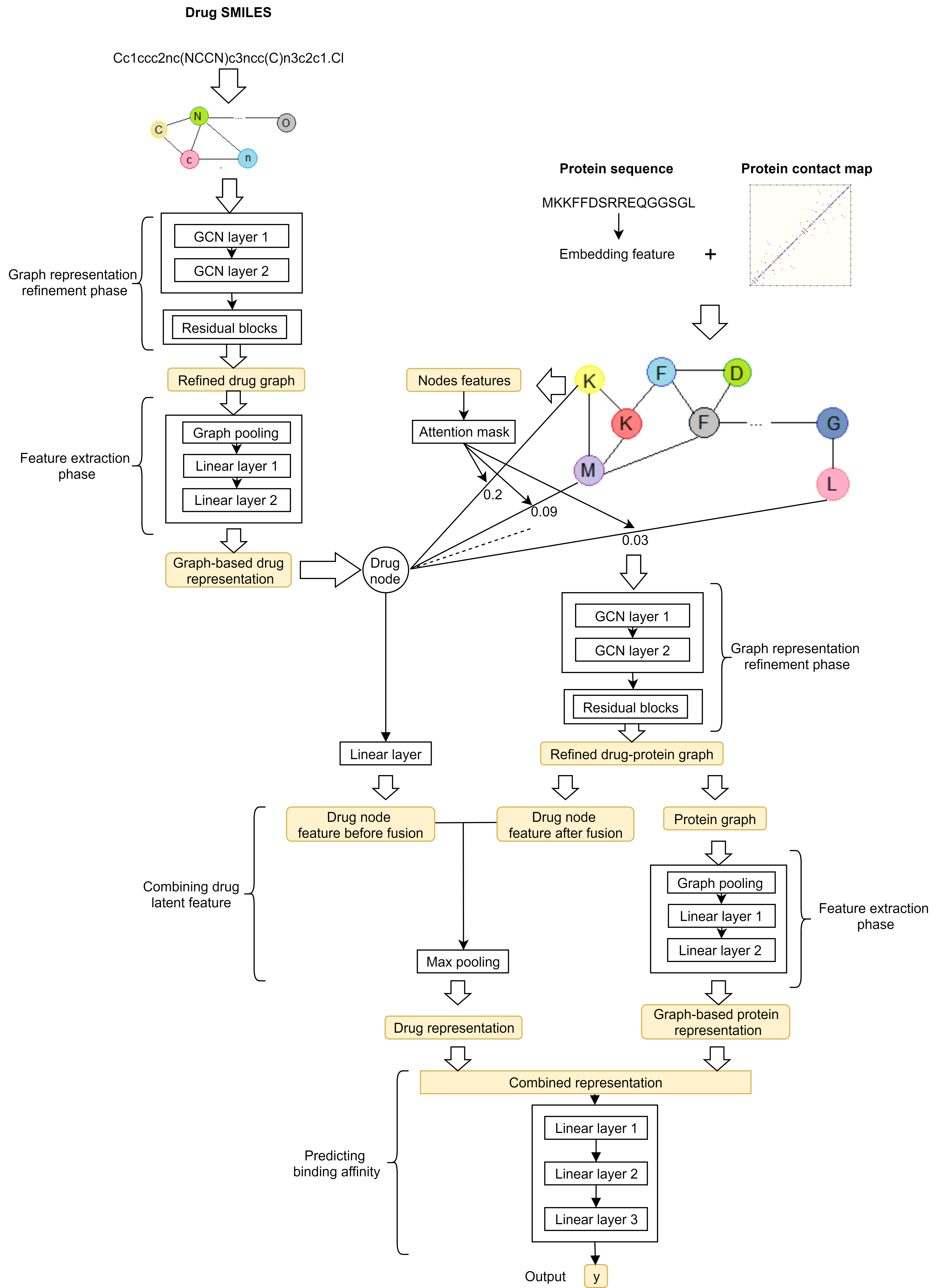
Figure 1: Illustration of Graph Early Fusion for binding Affinity prediction (GEFA). The GEFA takes as input the graph representations of a drug molecule and a protein target. We first use graph convolution network (GCN) for the drug graph feature refinement before applying a max pooling operator to obtain the estimated representation of the entire drug graph. The drug estimated vector is then used as an additional node to the protein graph, establishing graph-in-graph representation across domains. Information retrieved from the drug-protein graph along with the drug representation are finally used as the input for predicting the binding affinities between the given drug molecule and the protein target.

The overall architecture of our proposed method is presented in Fig.1. Our GEFA takes as input the graph structure of drug $\mathcal{G}_{d}$ and the graph structure of target $\mathcal{G}_{p}$ and outputs the prediction of binding affinity. We use Graph Convolutional Network (GCN) [49] for graph representation. In addition, we also make use of the well-known residual skip connection trick to make use of very deep GCNs.

3.3.1 Graph Convolutional Network

GCN is a convolutional network designed specifically for graph-structured signals. The goal is learn the node-level representation from a given input graph $\mathcal{G}=(\mathcal{X},\mathcal{A})$ where $\mathcal{X}$ is node feature matrix of $N$ nodes and $\mathcal{A}\in R^{N\times N}$ is the adjacency matrix that describes the graph structure. Let $W^{l}$ be the weight matrix at $l$-th layer, the graph convolution operation is defined by:

$$H^{1} =\mathcal{X},$$ (2)

$$H^{l} =\sigma\left(\tilde{D}^{-\frac{1}{2}}\tilde{\mathcal{A}}\tilde{D}^{-\frac{1}{2}}H^{l-1}W^{l-1}\right),$$ (3)

where $\mathcal{\tilde{A}=\mathcal{A}+I}$ is the adjacency matrix with self-loop in each node. $\mathcal{I}$ is the identity matrix and $\tilde{D}=\sum_{j}\mathcal{\tilde{A}}_{ij}$ and $\sigma$ is a non-linear function which is a ReLU [50] in our later experiments.

3.3.2 Deeper GCN with Residual Blocks

In general, a deeper model can generalize better and more compact than shallow networks[51]. However, stacking the vanilla GCN often suffers from the problem of gradient vanishing and numerical instability as a consequence of matrix multiplication in Eq. 3. To mitigate this problem, we use the GCN with residual skip-connection proposed in [52]. Similar to the effect of the residual block in the well-known CNN [53], skip connection in GCN helps to create more direct gradient flow, hence, allows to go deeper with more convolution layers. Mathematically, the graph convolution operation is given by:

$$H^{1}= \mathcal{X},$$ (4)

$$F^{l}(H^{l-1})= W_{2}^{l-1}\sigma(\mathcal{A}H^{l-1}W_{1}^{l-1}+b^{l-1}),$$ (5)

$$H^{l}= \sigma(H^{l-1}+F^{l}(H^{l-1})),$$ (6)

where $W_{1},W_{2}$ are learnable weight matrices, $l$ is layer-wise index and $\sigma$ is a non-linear function which is a ReLU activation function.

3.3.3 Graph-Graph Integration with Early Fusion

To reflect the changes in representation of a target protein due to the interaction between drug molecule and protein, we propose Graph Early Fusion for binding Affinity (GEFA), a method for migrating the drug molecule graph $\mathcal{G}_{d}=(\mathcal{V}_{d},\mathcal{A}_{d})$ into the protein graph $\mathcal{G}_{p}=(\mathcal{V}_{p},\mathcal{A}_{p})$ via a self-attention mechanism.

We first refine node representations in the drug graph with a two-layers GCN as in Eq. 3 and residual blocks as in Eq. 4, 5, 6. Let $\mathcal{V}_{d}^{\prime}=\{v_{i}^{\prime}\mid v_{i}^{\prime}\in R^{h_{1}}\}_{i=1}^{S}$ as node features of the drug graph after GCN, where $S$ is number of nodes in the drug graph. Note that $v_{i}^{\prime}$ contains aggregating information from its neighbors so we simply use the largest estimated representation of the refined drug graph as the representation of the entire graph. This is easily obtained by a max pooling operation followed by two linear layers for feature projection:

$$v_{\textrm{max}}^{\prime}=\textrm{MaxPool}(\mathcal{V}_{d}^{\prime}),$$ (7)

$$x_{d}=(W_{0}v_{\textrm{max}}^{\prime}+b_{0})W_{1}+b_{1}.$$ (8)

We call the resulted vector $x_{d}\in R^{h_{1}}$ as the drug molecules node, where $h_{1}$ is dimension of $x_{d}$.

We now explain how we integrate the drug molecules node $x_{d}$ into the protein graph $\mathcal{G}_{p}=(\mathcal{V}_{p},\mathcal{A}_{p})$ which is the main contribution of our work. The key idea is to use the drug node $x_{d}$ as an additional node that binds to the target graph $\mathcal{G}_{p}$. The edges connecting the drug node and residue nodes in the protein graph indicate the interaction between residues and drug molecule as well as the binding site. Since not every residue contributes equally to the binding affinity, the edge weights indicate the level of interactions of each residue with the drug molecule. To learn the level of contribution, we utilize a self-attention mechanism driven by the residue features $\mathcal{V}_{p}=\{v_{i}\mid v_{i}\in R^{h_{2}}\}_{i=1}^{L}$, recalling that $L$ is the length of the protein sequence. The self-attention mechanism is motivated from the fact that the binding site of the protein depends on the protein structure. In the other word, the attention weights tell which residues are more likely to participate in the binding process. Mathematically, the attention weights are given by:

$$\alpha_{i}=\textrm{sotfmax}(W_{2}\textrm{tanh}(W_{1}v_{i})),$$ (9)

where $\sum_{i=1}^{L}\alpha_{i}=1,v_{i}$ is the $i$-th residue feature, and $W_{1}$ and $W_{2}$ are the learnable parameters.

Given the drug node $x_{d}$ and its connections to residues in the target protein graph $\mathcal{G}_{p}$ denoted by $\{\alpha_{i}\}_{i=1}^{L}$, we now construct a cross-domain graph $\mathcal{G}_{pd}=\{\mathcal{V}_{pd},\mathcal{A}_{pd}\}$ where $\mathcal{V}_{pd}=\{\mathcal{V}_{p},x_{d}\}$ and $\mathcal{A}_{pd}=\{\mathcal{A}_{p},\{\alpha_{i}\}_{i=1}^{L}\}$. Similar to what we have done with the drug graph earlier, we employ a two-layers GCN followed by residual blocks to refine the node representations of the drug-protein graph $\mathcal{G}_{pd}$.

Before performing the graph feature extraction, the drug node after fusion $v_{dp}^{\prime}$ in the refined nodes $\mathcal{V}_{pd}^{\prime}$ by GCNs is taken out from the protein graph to ensure that the graph feature only contains residues nodes. Eventually, we extract the latent representation of the protein graph with a global max pooling operator followed by a two-layer linear network:

$$v_{\textrm{max}}^{\prime}=\textrm{MaxPool}(\mathcal{V}_{p}^{\prime}),$$ (10)

$$v_{pd}=(W_{0}v_{\textrm{max}}^{\prime}+b_{0})W_{1}+b_{1},$$ (11)

where $\mathcal{V}_{p}^{\prime}=\{\mathcal{V}_{pd}^{\prime}\setminus v_{dp}^{\prime}\}$ is the node representations of the protein graph after removing the drug node.

At the same time, the drug latent vector $x_{d}$ is transformed into the same dimensional space with $v_{dp}^{\prime}$ via a linear transformation. We further obtain the final representation of drug by combining these two features with a simple concatenation operator.

$$v_{db}=[x_{d};v_{dp}^{\prime}],$$ (12)

where $[\ ;]$ denotes the concatenation operation of two vectors. A max-pooling operation is then performed along the channel dimension to obtain the combined drug representation.

$$v_{dc}=\textrm{MaxPool}(v_{db}).$$ (13)

Consequently, the drug vector $v_{dc}$ and the protein latent vector $v_{pd}$ are concatenated and finally fed into a predictor of three fully connected layers to predict the binding affinities.

We wish to hypothesize that our early fusion approach with self-attention has two benefits. First, the early fusion approach explicitly models interactions between the drug graph and the target protein graph. Second, the self-attention allows the learning model to be more interpretable by showing which residues interact with drug molecules and how much they contribute to the binding process. We will back these in our later experiments.

4 Experiments

We evaluate our proposed model GEFA on Davis dataset[16] and compare against a late fusion baseline as well as state-of-the-art methods including GCNConvNet [7], GINConvNet [7], DGraphDTA [14]. Among those methods, GCNConvNet and GINConvNet use protein sequence and drug molecule graph as the input while DGraphDTA uses a protein graph built from contact and drug molecule as the input. We present the qualitative results in Sec. 4.1 and further provide analysis of our proposed model via extensive ablation studies in Sec.4.2.

4.1 Quantitative Experiments

4.1.1 Dataset

Davis dataset consists of binding affinity information between 72 drugs and 442 targets. The binding affinity between drug and target is measured by $K_{D}$ (kinase dissociation constant) value [16]. For the Davis dataset, the drug SMILES sequence of 68 drugs and the target protein sequence of 442 targets from DeepDTA[6] training/test set are used in our experiments.

There are four experiments settings for four scenarios. The first experiment setting is the warm setting where both protein and drug are known to the model. In this case, every protein and drug appear in training, validation, and test set.

The second experiment is cold-target where proteins are unknown to the model and drugs are known to the model. This setting replicates the scenarios of drug repurposing for a novel target. In this case, each unique protein sequence only appears in training, validation, or test set. As targets in the cold-target setting are required to be unique in both train, validation, and test sets, targets having the same sequence are filtered out which results in 361 targets. The 361 targets are split at 0.8/0.2 ratio for training-validation/testing. Then the training set is split at 0.8/0.2 ratio for training/validation.

The third experiment setting is cold-drug where proteins are known to the model and drugs are unknown to the model. In this case, a unique drug only appears in training, validation, or test set. We conduct the same splitting procedure in cold-target but applying for drugs.

Finally, the last experiment setting is cold-drug-target where both drugs and proteins are unknown to the model. This scenario is the case of novel drugs for the novel target. In this setting, we conduct the splitting procedure for both drug and target to ensure training, validation, and testing set do not share any common drug or target.

4.1.2 Implementation Details

Our methods are implemented using Pytorch. The protein sequence embedding features are extracted using TAPE-Protein [54]. The contact map is predicted by RaptorX [55]. The TAPE-Protein uses BERT language modelling [15]. The output of TAPE-Protein embedding features extraction is a embedding vector size 768. The graph convolution network uses the Pytorch geometric library [56]. The model are trained on $128$ mini-batch. The learning rate is $0.0005$ in warm setting. In cold-target, cold-drug, and cold-drug-target setting, the learning rate is $0.001$ as higher learning rate helps model to have better generalization and less likely to overfit. The learning rate decay is used. The learning rate is reduced by $20\%$ every $40$ epochs without improvement in MSE metric in the validation set. Adam optimizer is used. The model is trained in $1000$ epochs.

4.1.3 Evaluation Metrics

The models’ performances are evaluated using Concordance Index (CI)[57], Mean Squared Error (MSE), Root Mean Squared Error (RMSE), Pearson[58], and Spearman[59]. CI measures the quality of the ranking. CI formula is given as:

$$CI=\frac{1}{Z}\sum_{d_{i}>d_{j}}h(b_{i}-b_{j}),$$ (14)

$$h(x)=\begin{cases}1,&\text{if}\ x>0\\ 0.5,&\text{if}\ x=0\\ 0,&\text{if}\ x<0\end{cases},$$ (15)

where $b_{i}$ is the predicted value for the larger affinity value $d_{i}$, $b_{j}$ is the predicted value for the smaller affinity value $d_{j}$, Z is the normalization constant, and $h(x)$ is the step function.

MSE measures the mean squared error of the predicted values. MSE formula is given as:

$$MSE=\frac{1}{N}\sum_{i=1}^{N}(p_{i}-y_{i})^{2},$$ (16)

where $p_{i}$ is the predicted value and $y_{i}$ is the ground truth. RMSE is the square root of MSE.

Pearson measures the linear correlation between the predicted value $p$ and the ground truth $y$:

$$Pearson=\frac{\phi(p,y)}{\phi(p)\phi(y)},$$ (17)

where $\phi(p,y)$ is the covariance between the predicted value and the ground truth.

Spearman measures the rank correlation:

$$Spearman=1-\frac{6\sum_{i=1}^{n}d_{i}^{2}}{n(n^{2}-1)},$$ (18)

where $d_{i}$ is the difference between two ranks in the predicted values and ground truths.

4.1.4 Results

To compare our early fusion approach with the conventional late fusion approach, we provide a late fusion baseline model. Our late fusion baseline model (GLFA - Graph Late Fusion for binding Affinity) follows the convention model in which drug and protein representation are learned separately. GLFA has graph structures of drug and target as the input. Both graph structures are processed using the two-layers GCN and residual blocks in parallel to learn the hidden features. Then, the latent features are obtained by global max pooling followed by two linear layers. The latent features from both protein and drug are concatenated before under-going three fully connected layers. The output of the final fully connected layers is the binding affinity value of the input drug and target protein. The late fusion model is a special case of early fusion where all drug-residues edge weights are set to 0. The late fusion approach is used as baseline to compare with our proposed early fusion approach.

TABLE I: The result of quantitative experiments

Architecture	RMSE$\downarrow$	MSE$\downarrow$	Pearson$\uparrow$	Spearman$\uparrow$	CI $\uparrow$
Warm start setting
GCNConvNet [7]	0.5331	0.2842	0.8043	0.6609	0.8649
GINConvNet [7]	0.50723	0.2573	0.8245	0.6818	0.8785
DGraphDTA [14]	0.4917	0.2417	0.8378	0.7001	0.8869
GLFA	0.4850	0.2353	0.8412	0.7073	0.8950
GEFA	0.4775	0.2280	0.8467	0.7023	0.8927
Cold-target setting
GCNConvNet [7]	0.7071	0.5000	0.5145	0.4316	0.7293
GINConvNet [7]	0.7144	0.5104	0.5166	0.3904	0.7065
DGraphDTA [14]	0.6855	0.4700	0.5597	0.4941	0.7656
GLFA	0.6732	0.4531	0.5828	0.5228	0.7802
GEFA	0.6584	0.4335	0.6030	0.5506	0.7951
Cold-drug setting
GCNConvNet [7]	0.9723	0.9454	0.3385	0.3764	0.6784
GINConvNet [7]	0.9592	0.9200	0.3779	0.3693	0.6758
DGraphDTA [14]	0.9583	0.9184	0.3610	0.3150	0.5337
GLFA	0.9280	0.8612	0.4023	0.3549	0.6703
GEFA	0.9202	0.8467	0.4515	0.4320	0.7091
Cold-drug-target setting
GCNConvNet [7]	1.0632	1.1304	0.1904	0.1698	0.5782
GINConvNet [7]	1.0651	1.1345	0.1974	0.2763	0.6275
DGraphDTA [14]	1.0749	1.1554	0.0228	0.1795	0.6081
GLFA	1.0698	1.1444	0.3473	0.2901	0.6362
GEFA	0.9949	0.9899	0.3148	0.2932	0.6390

We report our late fusion approach, GLFA, and early fusion approach, GEFA, with previous works in Davis benchmark on four settings in Table I. Our proposed method GEFA consistently outperforms previous works in four settings. Our proposed methods achieve state-of-the-art performance across all four settings. Between two late fusion based methods DGraphDTA [14] and GLFA, our proposed GLFA method also outperforms DGraphDTA. This follows our expectations as the embedding feature contains richer information than one-hot encoding and PSSM. This also demonstrates the advantage of using the residual block.

DgraphDTA [14], GLFA, and GEFA outperform GINConvNet in all four settings. GINConvNet and GCNConvNet [7] only use sequence and CNN to learn the target representation. On the other hand, DgraphDTA [14], GLFA, and GEFA use the graph built from the protein contact map and learn the target representation using GCN. This demonstrates the advantage of using the graph representation of the contact map.

Between our two proposed methods GEFA and GLFA, the early fusion method GEFA shows advantages over late fusion method GLFA. This follows our expectation as the early fusion allows interactions between drug and protein graph during the graph representation learning phase for more accurate latent representation.

We can observe a common trend that all models performances in the cold-drug setting are lower than performance in the cold-target setting. The reason is that the number of unique target sequences in Davis dataset is higher than the number of unique SMILES sequence. Therefore, models have more target protein samples to learn the feature space of the protein.

4.2 Ablation Studies

To understand the contribution of each component to the overall performance in the early fusion GEFA model, we remove each component from the GEFA model. We conduct the ablation experiment using the Davis dataset benchmark in the warm setting.

First, we evaluate the usage of the embedding feature by comparing it with the one-hot encoding.

Second, we evaluate the usage of attention mask as the graph edge. Instead of using attention as drug-residue edge weight, drug-residue edges are weighted the same as the residue-residue edges in the target graph.

Third, we evaluate the usage of the 2-layer GCN and the usage of residual blocks to refine graph structure. As all residual blocks have shared weight, this reduces the number of parameters, which may help in the case of over-fitting.

Fourth, we evaluate the residual blocks. We test three cases: without residual blocks in both protein and drug graph, without protein graph residual blocks, and without drug graph residual blocks.

Finally, we compare the drug representation extracted from the drug-protein fusion graph and drug representation extracted from the drug graph. Instead of fusing two types of drug features followed by pooling, we only use one type of drug feature to combine with graph-based protein representation.

TABLE II: The result of experiment warm setting with different component in Davis dataset in warm setting. The first row shows proposed GEFA with all components.)

Architecture	RMSE$\downarrow$	MSE$\downarrow$	Pearson$\uparrow$	Spearman$\uparrow$	CI $\uparrow$
GEFA	0.4775	0.2280	0.8467	0.7023	0.8927
One-hot encoding	0.5050	0.2551	0.8274	0.6919	0.8837
W/o attention	0.4887	0.2388	0.8392	0.7014	0.8909
W/o 2-layer GCN	0.4844	0.2346	0.8425	0.6933	0.887
Residual blocks usage
W/o residual blocks	0.4933	0.2434	0.8351	0.686	0.8819
Drug graph res. blocks	0.4944	0.2444	0.8351	0.6874	0.8828
Protein graph res. blocks	0.4873	0.2375	0.8407	0.7045	0.8941
Drug representation choice
Before fusion rep.	0.4806	0.231	0.8448	0.7058	0.8954
After fusion rep.	0.5171	0.2673	0.8174	0.6437	0.8558

As shown in Table. II, model using the protein embedding feature has an improvement of $11.85\%$ in MSE and $1.00\%$ in CI. This emphasizes the advantage of using the protein embedding feature as the graph node feature.

Using attention mask as the drug-residue edge in protein graph gains improvement of $4.74\%$ in MSE and $0.20\%$ in CI. Without the attention mask, we assume that the drug molecule interacts with all residues in target protein equally. However, each residue contributes differently to the binding process. Therefore, it is reasonable to use self-attention to learn each residue’s contribution level which is used as edge weight between drug node and residue node.

Using the 2-layers GCN (GEFA in Table. II) shows improvement compared to without using 2-layer GCN (w/o using the 2-layers GCN in Table. II). Compared to the model using solely residual blocks as graph refinement (w/o 2-layer GCN in Table. II), the model with residual block shows an advantage over the model with only the 2-layers GCN (w/o graph residual blocks in Table. II). Therefore, it can be suggested that residual blocks have the same or even better learning ability than the 2-layer GCN. Interestingly, combining both the 2-layers GCN and residual blocks brings the best result as shown in the full component model GEFA.

The model using residual blocks in both drug and protein graph shows an advantage over the model without any residual blocks. Model having residual blocks for both drug graph and protein graph gains $6.73\%$ improvement in MSE over the model without residual blocks. It is interesting that applying residual blocks only for drug graph slightly decrease model performance (0.2% decrease in MSE and 0.1% decrease in CI). Adding back residual blocks for protein graph helps the model to gain $2.43\%$ improvement in MSE. Stacking residual blocks in protein graph is more crucial in the early fusion approach as it affects not only protein graph representation but also the drug node representation.

Finally, we compare the drug representation before and after the drug-target graph fusion. Model using only drug representation before fusion shows comparable performance while the model using drug representation after fusion suffers $17.24\%$ performance loss in MSE. This indicates that drug representation before fusion is more useful than after fusion. The reason is likely due to message passing in graph neural network. The drug node info is updated from its neighbor residue nodes. Therefore, this suggests that the binding process does not bring any signification change to the ligand latent representation.

4.3 Error Analysis

We analyze how protein sequences are clustered and their effect on model performance. First, we cluster target sequences based on BLAST+ similarities using CLANS [60] convex clustering on a 2D plane. Five major clusters having more than 10 targets are chosen to analyze the model performance. The distribution of five clusters in 2D is shown in Fig. 2. The average absolute errors of five major clusters are displayed in Fig. 3 and Table. III. As shown in Fig. 2, cluster 1, 2, 3, and 5 are close to each other in the 2D similarity distribution space. The average error of cluster 1, 2, 3, and 5 are roughly the same at $0.2\%$. On the other hand, cluster 4 has a high distance to other clusters. There is a significant difference in model performance in cluster 4 compared to other clusters. There are two possible explanations. First, good performance is from the over-representation of specific targets in the training set. However, this is not the case as in all five clusters the training sample/testing sample ratio is nearly the same at $0.8/0.2$. Second, the difference in performance is likely due to some specific characteristics of the cluster such as sequence length, motif, etc.

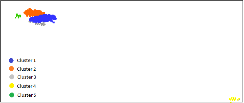
Figure 2: The distribution of five major target sequence clusters.

Figure 3: The average absolute error of each target by five major clusters.

TABLE III: The number of training and testing samples, the number of protein, and average absolute error of five major sequence clusters.)

Cluster	No pairs in testing	No pairs in training	Train/test ratio	No proteins	Average absolute error
1	2159	10952	0.1971	192	0.2137 $(\pm 0.1492)$
2	1519	7455	0.2037	132	0.2882 $(\pm 0.2059)$
3	202	1022	0.1977	18	0.2189 $(\pm 0.0849)$
4	188	900	0.2089	16	0.0386 $(\pm 0.1166)$
5	117	563	0.2078	10	0.1923 $(\pm 0.1449)$

We analyze the binding site predicted by the GEFA model in the successful case and the failed case. We choose two drug-target binding pairs with 3D structure available having the lowest and highest absolute error. For the successful case, we analyze the binding between target MST1 and compound Bosutinib (PubChem CID 5328940) predicted by our proposed model and compare it with blind docking simulation [61]. The Bosutinib-MST1 pair has predicted $K_{D}$ value at 6.72132 with the absolute error at 0.0000738.

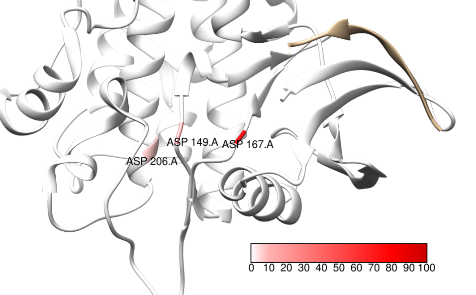
Figure 4: Attention values at predicted binding sites of MST1 target. The attention value at residue ASP 149.A is 0.2 (20%) , 0.72 (72%) at residue ASP 167.A, and 0.07 (7%) at residue ASP 206.A

Figure 5: Residue-ligand interaction between MST1 and Bosutinib predicted by blind docking.

Figure 6: Predicted binding pocket highlighted in red and the Bosutinib ligand docking

The attention value from the self-attentive layer of the MST1 target indicates that the residue ASP 167.A has the highest probability (0.72) to be the binding site. This agrees with the blind docking result. In the blind docking simulation of the Bosutinib-MST1 pair, the conformation with the lowest binding energy ($-7.30kcal/mol$) shows the hydrogen bond between ASP 167.A and the ligand (Fig. 5).

For the failed case, we analyze the binding between target EGFR(T790M) and Lapatinib (PubChem CID 208908). The predicted $K_{D}$ value is 8.7785 while the ground truth value is 6.0655. The attention value obtained from the self-attentive layer peaks at ASP 896.A with 0.48 (48%) confidence (see Fig. 7). However, in the crystallised structure of EGFR(T790M), the 896.A residue is buried (see Fig.8) and is less likely to be the binding site. In addition, the predicted conformation of blind docking shows no interaction between residue 896.A and the ligand (see Fig. 9). Therefore, in the early fusion model, the edges between the drug node and binding site residue are not correct. As a result, the error of the predicted $K_{D}$ value of Lapatinib-EGFR(T790M) is one of the highest in the Davis test set. From two examples of a successful case and failed case, obtaining the correct binding site to form the correct drug node - residues edge is one of the important aspects of the early fusion approach.

Figure 7: Attention values at predicted binding sites of EGFR(T790M) target.

Figure 8: Solvent-excluded surface areas value of EGFR(T790M) target.

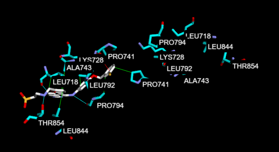
Figure 9: Residue-ligand interaction between EGFR(T790M) and Lapatinib predicted by blind docking.

5 Conclusion

We have proposed a novel deep learning method, called GEFA (Graph Early Fusion for binding Affinity prediction) for target-drug affinity prediction, a crucial task for rapid virtual drug screening and drug repurposing. To improve the power of protein representation, we use self-supervised to take advantage of a large amount of unlabeled target sequences. To address the latent representation change due to conformation change during the binding process, the early fusion between drug and target is proposed. Unlike the late fusion approach extracting representation separately, the early fusion approach integrates drug representation info into protein representation learning phase. The self-attention value of the target sequence is used as edge weight connecting drug node and residue node in the target protein graph. Self-attention allows the model more interpretable as it shows which residues contribute to the binding process and the level of contribution of each residue. The quantitative experiments show that the early fusion approach has advantages over the late fusion approach. Using the embedding feature as target node feature has advantages over using one-hot encoding. Residual block design allows stacking multiple GCN layers for better learning representation capability.

This work opens room for future investigations. Even though the target representation change is addressed by adding drug node to the target graph during the representation learning phase, the conformation change, which is the residue-residue edge connection change, is not addressed. If we can learn the edge change, we can express the conformation change caused by the drug-target binding. In addition, in case the target protein has multiple binding pocket at different regions, the drug molecule may only bind at one pocket at one time. However, in our model, the drug node links to all possible binding sites indicated by self-attention mask. The binding process modeling will be more accurate if we can combine drug info into the finding drug-residues edges process.

Tri Minh Nguyen is a PhD student at Deakin University. His research interest is applying machine learning in studying the protein structure and function. He is exploring the application of energy-based models in protein structure and function.

Thin Nguyen is a Senior Research Fellow with the Applied Artificial Intelligence Institute (A2I2), Deakin University, Australia. He graduated with a PhD in Computer Science from Curtin University, Australia. His current research topic is inter-disciplinary, bridging large-scale data analytics, pattern recognition, genetics and medicine. His research direction is to develop machine learning methods to discover functional connections between drugs, genes and diseases.

Thao Minh Le is a senior PhD student at Applied Artificial Intelligence Institute, Deakin University. His research interests focus on computer vision and its applications, and machine reasoning. He is currently exploring new frontiers in learning and reasoning across different modalities.

Truyen Tran is an Associate Professor at Deakin University. He is member of Applied Artificial Intelligence Institute where he leads the work on deep learning and its application on health, genomics, software and materials science. His other research topics include probabilistic graphical models, recommender systems, learning to rank, anomaly detection, multi-relational databases, model stability, and mixed-type analysis.

References

- [1] Maha Thafar et al. “Comparison Study of Computational Prediction Tools for Drug-Target Binding Affinities” In Frontiers in Chemistry 7 Frontiers Media SA, 2019
- [2] Sunghwan Kim et al. “PubChem 2019 update: improved access to chemical data” In Nucleic Acids Research 47.D1 Oxford University Press, 2019, pp. D1102–D1109
- [3] Michael K Gilson et al. “BindingDB in 2015: a public database for medicinal chemistry, computational chemistry and systems pharmacology” In Nucleic Acids Research 44.D1 Oxford University Press, 2016, pp. D1045–D1053
- [4] Anna Cichonska et al. “Computational-experimental approach to drug-target interaction mapping: a case study on kinase inhibitors” In PLOS Computational Biology 13.8 Public Library of Science, 2017, pp. e1005678
- [5] Anna Cichonska et al. “Learning with multiple pairwise kernels for drug bioactivity prediction” In Bioinformatics 34.13 Oxford University Press, 2018, pp. i509–i518
- [6] Hakime Öztürk, Arzucan Özgür and Elif Ozkirimli “DeepDTA: deep drug–target binding affinity prediction” In Bioinformatics 34.17 Oxford University Press, 2018, pp. i821–i829
- [7] Thin Nguyen, Hang Le and Svetha Venkatesh “GraphDTA: prediction of drug–target binding affinity using graph convolutional networks” In bioRxiv Cold Spring Harbor Laboratory, 2019, pp. 684662
- [8] Hakime Öztürk, Elif Ozkirimli and Arzucan Özgür “WideDTA: prediction of drug-target binding affinity” In arXiv preprint arXiv:1902.04166, 2019
- [9] Zhan-Chao Li et al. “Identification of drug–target interaction from interactome network with ‘guilt-by-association’ principle and topology features” In Bioinformatics 32.7 Oxford University Press, 2016, pp. 1057–1064
- [10] Sheng Wang, Siqi Sun and Jinbo Xu “Analysis of deep learning methods for blind protein contact prediction in CASP12” In Proteins: Structure, Function, and Bioinformatics 86 Wiley Online Library, 2018, pp. 67–77
- [11] Andrew W Senior et al. “Improved protein structure prediction using potentials from deep learning” In Nature 577.7792 Nature Publishing Group, 2020, pp. 706–710
- [12] Shuangjia Zheng et al. “Predicting drug–protein interaction using quasi-visual question answering system” In Nature Machine Intelligence 2.2 Nature Publishing Group, 2020, pp. 134–140
- [13] Simon J Teague “Implications of protein flexibility for drug discovery” In Nature Reviews Drug discovery 2.7 Nature Publishing Group, 2003, pp. 527–541
- [14] Mingjian Jiang et al. “Drug–target affinity prediction using graph neural network and contact maps” In RSC Advances 10.35 Royal Society of Chemistry, 2020, pp. 20701–20712
- [15] Jacob Devlin, Ming-Wei Chang, Kenton Lee and Kristina Toutanova “BERT: Pre-training of Deep Bidirectional Transformers for Language Understanding” In Proceedings of the 2019 Conference of the North American Chapter of the Association for Computational Linguistics: Human Language Technologies, pp. 4171–4186
- [16] Mindy I Davis et al. “Comprehensive analysis of kinase inhibitor selectivity” In Nature Biotechnology 29.11 Nature Publishing Group, 2011, pp. 1046–1051
- [17] Joris Langedijk, Aukje K Mantel-Teeuwisse, Diederick S Slijkerman and Marie-Hélène DB Schutjens “Drug repositioning and repurposing: terminology and definitions in literature” In Drug Discovery Today 20.8 Elsevier, 2015, pp. 1027–1034
- [18] Hanqing Xue, Jie Li, Haozhe Xie and Yadong Wang “Review of drug repositioning approaches and resources” In International Journal of Biological Sciences 14.10 Ivyspring International Publisher, 2018, pp. 1232
- [19] Sudeep Pushpakom et al. “Drug repurposing: progress, challenges and recommendations” In Nature Reviews Drug Discovery 18.1 Nature Publishing Group, 2019, pp. 41–58
- [20] Mani P Grover et al. “Novel therapeutics for coronary artery disease from genome-wide association study data” In BMC Medical Genomics 8.S2 Springer, 2015, pp. S1
- [21] Philippe Sanseau et al. “Use of genome-wide association studies for drug repositioning” In Nature Biotechnology 30.4 Nature Publishing Group, 2012, pp. 317
- [22] Francesco Iorio, Antonella Isacchi, Diego Bernardo and Nicola Brunetti-Pierri “Identification of small molecules enhancing autophagic function from drug network analysis” In Autophagy 6.8 Taylor & Francis, 2010, pp. 1204–1205
- [23] Francesco Iorio, Julio Saez-Rodriguez and Diego Di Bernardo “Network based elucidation of drug response: from modulators to targets” In BMC Systems Biology 7.1 BioMed Central, 2013, pp. 1–9
- [24] Steven B Smith et al. “Identification of common biological pathways and drug targets across multiple respiratory viruses based on human host gene expression analysis” In PLOS One 7.3 Public Library of Science, 2012, pp. e33174
- [25] MR Hurle et al. “Computational drug repositioning: from data to therapeutics” In Clinical Pharmacology & Therapeutics 93.4 Wiley Online Library, 2013, pp. 335–341
- [26] Peter B Jensen, Lars J Jensen and Søren Brunak “Mining electronic health records: towards better research applications and clinical care” In Nature Reviews Genetics 13.6 Nature Publishing Group, 2012, pp. 395–405
- [27] Hyojung Paik et al. “Repurpose terbutaline sulfate for amyotrophic lateral sclerosis using electronic medical records” In Scientific Reports 5 Nature Publishing Group, 2015, pp. 8580
- [28] Joel T Dudley, Tarangini Deshpande and Atul J Butte “Exploiting drug–disease relationships for computational drug repositioning” In Briefings in Bioinformatics 12.4 Oxford University Press, 2011, pp. 303–311
- [29] Francesco Iorio et al. “Transcriptional data: a new gateway to drug repositioning?” In Drug Discovery Today 18.7-8 Elsevier, 2013, pp. 350–357
- [30] Marina Sirota et al. “Discovery and preclinical validation of drug indications using compendia of public gene expression data” In Science Translational Medicine 3.96 American Association for the Advancement of Science, 2011, pp. 96ra77–96ra77
- [31] Douglas B Kitchen, Hélène Decornez, John R Furr and Jürgen Bajorath “Docking and scoring in virtual screening for drug discovery: methods and applications” In Nature Reviews Drug Discovery 3.11 Nature Publishing Group, 2004, pp. 935–949
- [32] Sivanesan Dakshanamurthy et al. “Predicting new indications for approved drugs using a proteochemometric method” In Journal of Medicinal Chemistry 55.15 ACS Publications, 2012, pp. 6832–6848
- [33] Robert M Cooke, Alastair JH Brown, Fiona H Marshall and Jonathan S Mason “Structures of G protein-coupled receptors reveal new opportunities for drug discovery” In Drug Discovery Today 20.11 Elsevier, 2015, pp. 1355–1364
- [34] Weina Ma, Liu Yang and Langchong He “Overview of the detection methods for equilibrium dissociation constant KD of drug-receptor interaction” In Journal of Pharmaceutical Analysis 8.3 Elsevier, 2018, pp. 147–152
- [35] Elaine C Meng, Brian K Shoichet and Irwin D Kuntz “Automated docking with grid-based energy evaluation” In Journal of Computational Chemistry 13.4 Wiley Online Library, 1992, pp. 505–524
- [36] William L Jorgensen et al. “Comparison of simple potential functions for simulating liquid water” In The Journal of Chemical Physics 79.2 American Institute of Physics, 1983, pp. 926–935
- [37] A Pullman “Intermolecular forces” Springer Science & Business Media, 2013
- [38] Kaushik Raha et al. “The role of quantum mechanics in structure-based drug design” In Drug Discovery Today 12.17-18 Elsevier, 2007, pp. 725–731
- [39] Indra Kundu, Goutam Paul and Raja Banerjee “A machine learning approach towards the prediction of protein–ligand binding affinity based on fundamental molecular properties” In RSC Advances 8.22 Royal Society of Chemistry, 2018, pp. 12127–12137
- [40] Marta M Stepniewska-Dziubinska, Piotr Zielenkiewicz and Pawel Siedlecki “Development and evaluation of a deep learning model for protein–ligand binding affinity prediction” In Bioinformatics 34.21 Oxford University Press, 2018, pp. 3666–3674
- [41] Joseph Gomes, Bharath Ramsundar, Evan N Feinberg and Vijay S Pande “Atomic convolutional networks for predicting protein-ligand binding affinity” In arXiv preprint arXiv:1703.10603, 2017
- [42] Tong He et al. “SimBoost: a read-across approach for predicting drug–target binding affinities using gradient boosting machines” In Journal of Cheminformatics 9.1 BioMed Central, 2017, pp. 1–14
- [43] Qingyuan Feng, Evgenia Dueva, Artem Cherkasov and Martin Ester “PADME: A deep learning-based framework for drug-target interaction prediction” In arXiv preprint arXiv:1807.09741, 2018
- [44] Wen Torng and Russ B Altman “Graph convolutional neural networks for predicting drug-target interactions” In Journal of Chemical Information and Modeling 59.10 ACS Publications, 2019, pp. 4131–4149
- [45] Jean-Jacques Lacapere, Eva Pebay-Peyroula, Jean-Michel Neumann and Catherine Etchebest “Determining membrane protein structures: still a challenge!” In Trends in Biochemical Sciences 32.6 Elsevier, 2007, pp. 259–270
- [46] UniProt Consortium “UniProt: a worldwide hub of protein knowledge” In Nucleic Acids Research 47.D1 Oxford University Press, 2019, pp. D506–D515
- [47] Roshan Rao et al. “Evaluating protein transfer learning with TAPE” In Advances in Neural Information Processing Systems, 2019, pp. 9689–9701
- [48] Longlong Jing and Yingli Tian “Self-supervised visual feature learning with deep neural networks: A survey” In IEEE Transactions on Pattern Analysis and Machine Intelligence IEEE, 2020
- [49] Thomas N. Kipf and Max Welling “Semi-Supervised Classification with Graph Convolutional Networks” In Proceedings of 5th International Conference on Learning Representations, ICLR 2017
- [50] Abien Fred Agarap “Deep Learning using Rectified Linear Units (ReLU)” In arXiv preprint arXiv:1803.08375, 2018
- [51] Ian Goodfellow, Yoshua Bengio and Aaron Courville “Deep Learning” MIT Press, 2016
- [52] Thao Minh Le, Vuong Le, Svetha Venkatesh and Truyen Tran “Dynamic Language Binding in Relational Visual Reasoning” In Proceedings of the Twenty-Ninth International Joint Conference on Artificial Intelligence, IJCAI-20, pp. 818–824
- [53] Kaiming He, Xiangyu Zhang, Shaoqing Ren and Jian Sun “Deep residual learning for image recognition” In Proceedings of the IEEE Conference on Computer Vision and Pattern Recognition, 2016, pp. 770–778
- [54] Roshan Rao et al. “Evaluating Protein Transfer Learning with TAPE” In Advances in Neural Information Processing Systems, 2019
- [55] Sheng Wang et al. “Accurate de novo prediction of protein contact map by ultra-deep learning model” In PLOS Computational Biology 13.1 Public Library of Science San Francisco, CA USA, 2017, pp. e1005324
- [56] Matthias Fey and Jan E. Lenssen “Fast Graph Representation Learning with PyTorch Geometric” In Proceedings of ICLR Workshop on Representation Learning on Graphs and Manifolds, 2019
- [57] Mithat Gönen and Glenn Heller “Concordance probability and discriminatory power in proportional hazards regression” In Biometrika 92.4 Oxford University Press, 2005, pp. 965–970
- [58] Jacob Benesty, Jingdong Chen, Yiteng Huang and Israel Cohen “Noise reduction in speech processing” Springer Science & Business Media, 2009
- [59] Daniel Zwillinger and Stephen Kokoska “CRC standard probability and statistics tables and formulae” CRC Press, 1999
- [60] Tancred Frickey and Andrei Lupas “CLANS: a Java application for visualizing protein families based on pairwise similarity” In Bioinformatics 20.18 Oxford University Press, 2004, pp. 3702–3704
- [61] Irene Sánchez-Linares, Horacio Pérez-Sánchez, José M Cecilia and José M García “High-throughput parallel blind virtual screening using BINDSURF” In BMC Bioinformatics 13.S14 Springer, 2012, pp. S13