Pareto efficient combinatorial auctions:
dichotomous preferences without quasilinearity

Abstract

We consider a combinatorial auction model where preferences of agents over bundles of objects and payments need not be quasilinear. However, we restrict the preferences of agents to be dichotomous. An agent with dichotomous preference partitions the set of bundles of objects as acceptable and unacceptable, and at the same payment level, she is indifferent between bundles in each class but strictly prefers acceptable to unacceptable bundles. We show that there is no Pareto efficient, dominant strategy incentive compatible (DSIC), individually rational (IR) mechanism satisfying no subsidy if the domain of preferences includes all dichotomous preferences. However, a generalization of the VCG mechanism is Pareto efficient, DSIC, IR and satisfies no subsidy if the domain of preferences contains only positive income effect dichotomous preferences. We show tightness of this result: adding any non-dichotomous preference (satisfying some natural properties) to the domain of quasilinear dichotomous preferences brings back the impossibility result.

JEL Codes: D82, D90

Keywords: combinatorial auctions; non-quasilinear preferences; dichotomous preferences; single-minded bidders

1 Introduction

The Vickrey-Clarke-Groves (VCG) mechanism (Vickrey, 1961; Clarke, 1971; Groves, 1973) occupies a central role in mechanism design theory (specially, with private values). It satisfies two fundamental desiderata: it is dominant strategy incentive compatible (DSIC) and Pareto efficient. We study a model of combinatorial auctions, where multiple objects are sold to agents simultaneously, who may buy any bundle of objects. For such combinatorial auction models, the VCG mechanism and its indirect implementations (like ascending price auctions) have been popular. The VCG mechanism is also individually rational (IR) and satisfies no subsidy (i.e., does not subsidize any agent) in these models.

Unfortunately, these desirable properties of the VCG mechanism critically rely on the fact that agents have quasilinear preferences. While analytically convenient and a good approximation of actual preferences when payments involved are low, quasilinearity is a debatable assumption in practice. For instance, consider an agent participating in a combinatorial auction for spectrum licenses, where agents often borrow from various investors at non-negligible interest rates. Such borrowing naturally leads to a preference which is not quasilinear. Further, income effects are ubiquitous in settings with non-negligible payments. For instance, a bidder in a spectrum auction often needs to invest in telecom infrastrastructure to realize the full value of spectrum. Higher payment in the auction will lead to lower investments in infrastructure, and hence, a lower value for the spectrum.

This has initiated a small literature in mechanism design theory (discussed later in this section and again in Section 4), where the quasilinearity assumption is relaxed to allow any classical preference of the agent over consumption bundles: (bundle of objects, payment) pairs. The main research question addressed in this literature is the following:

In combinatorial auction models, if agents have classical preferences, is it possible to construct a “desirable" mechanism: a mechanism which inherits the DSIC, Pareto efficiency, IR, and no subsidy properties of the VCG mechanism?

1.1 Dichotomous preferences

This paper contributes to this literature, focusing on the particular case in which agents’ preferences belong to a class of preferences, which we call dichotomous. If an agent has a dichotomous preference, she partitions the set of bundles of objects into acceptable and unacceptable. If the payments for all the bundles of objects are the same, then an agent is indifferent between her acceptable bundles of objects; she is also indifferent between unacceptable bundles of objects; but she prefers every acceptable bundle to every unacceptable bundle.

Such preferences, though restrictive, are found in many settings of interest. For instance, consider the recent “incentive auction" done by the US Government (Leyton-Brown et al., 2017). It involved a “reverse auction" phase where the broadcast licenses from existing broadcasters were bought; a “forward auction" phase where buyers bought broadcast licenses; and a clearing phase. The auction resulted in billions of dollars in revenue for US treasury (Leyton-Brown et al., 2017). The theoretical analysis of the reverse auction phase was done by Milgrom and Segal (2020), where they assume quasilinear preferences with “single-minded" bidders, a specific kind of dichotomous preference where the bidder has a unique acceptable bundle (a broadcast band in this case). In these auctions, a broadcaster had some feasible frequency bands in which it can operate. Any of those feasible frequency bands were “acceptable” and it was indifferent between them (since any of these frequencies allowed the broadcaster to realize its full value of broadcast). This resulted in dichotomous preferences of agents. Milgrom and Segal (2020) argue that the VCG mechanism is computationally challenging in this setting and propose a simpler mechanism.

The assumption of dichotomous preferences seems natural in settings where a bidder is acquiring some resources, and finds any bundle acceptable if it satisfies some requirements. For instance, consider the following examples.

• Consider a scheduling problem, where a certain set of jobs (say, flights at the take-off slots of an airport) need to be scheduled on a server. There are certain intervals where each job is available and can be processed and other intervals are not acceptable. For instance, a supplier bidding to supply to a firm’s production schedule can do so only on some fixed interval of dates. So, certain dates are acceptable to it and others are not acceptable. A traveller is buying tickets between a pair of cities but find certain dates acceptable for travel and realize value only on those dates.

• Consider a seller who is selling land to different buyers. The lands differ in size but are homogeneous otherwise. Each buyer only demands a land of a fixed size. For instance, suppose the Government is allocating land to firms to set up factories in a region, and each firm needs a land of a fixed size to set up its factory. This means all the bundles of land exceeding the size requirement are acceptable to a firm.

• Consider firms (data providers) buying paths on (data) networks (Babaioff et al., 2009) - a firm is interested in sending data from node $x$ to node $y$ on a directed graph whose edges are up for sale, and as long as a bundle of edges contain a path from $x$ to $y$, it is acceptable to the firm.

In all the examples above, if the payment involved are high, we can expect income effects, which will mean that agents do not have quasilinear preferences. One may also consider the dichotomous preference restriction as a behavioural assumption, where the agent does not consider computing values for each of the exponential number of bundles but classifies the bundles as acceptable and unacceptable. Hence, they are easy to elicit even in combinatorial auction setting. Even with quasilinear preferences, the dichotomous restriction poses interesting combinatorial challenges for computing the VCG outcome. This has led to a large literature in computer science for looking at approximately desirable VCG-style mechanisms (Babaioff et al., 2005, 2009; Lehmann et al., 2002; Ledyard, 2007; Milgrom and Segal, 2014). Also related is the literature in matching and social choice theory (models without payments), where dichotomous preferences have been widely studied (Bogomolnaia and Moulin, 2004; Bogomolnaia et al., 2005; Bade, 2015).

1.2 Summary and intuition of results

We show that if the domain of preferences contains all dichotomous classical preferences, there is no desirable mechanism. However, a natural generalization of the VCG mechanism to classical preferences, which we call the generalized VCG (GVCG) mechanism, is desirable if the domain contains only positive income effect dichotomous preferences. In other words, when normal goods are sold, the GVCG mechanism is desirable. Further, the GVCG mechanism is the unique desirable mechanism in any domain of positive income effect dichotomous preferences if it contains the quasilinear dichotomous preferences. The GVCG mechanism allocates the goods in a way such that the collective willingness to pay of all the bidders is maximized. Classical preferences imply that willingness to pay for a bundle of objects depends on the payment level. Thus, it is not clear what the counterpart of “valuation" of a bundle of objects is in this setting. Our generalized VCG is defined by treating the willingness to pay at zero payment as the “valuation" of a bundle and then defining the VCG outcome with respect to these valuations, i.e., the allocation maximizes the sum of agents’ valuations and each agent pays her externality.

The intuition for these results is the following. The GVCG mechanism allocates the goods in a way that maximizes the collective willingness to pay of all the bidders. In fact, with enough richness in the domain, every desirable mechanism must allocate objects like the GVCG mechanism at certain profiles. Individual rationality implies that winning bidders pay an amount less than their willingness to pay. So, winning makes a winning bidder wealthier. With dichotomous preferences, the payments in the GVCG mechanism can be quite low. If bidders have negative income effect, then their willingness to sell (i.e., the compensating amount needed to make a winning bidder lose her bundle of objects) is lower than their willingness to pay. This creates ex-post trading opportunities and the GVCG mechanism is no longer efficient. On the other hand, with positive income effect, the willingness to sell of winning bidders is higher than their willingness to pay and the GVCG mechanism is efficient.

Our positive result is tight: we get back impossibility in any domain containing quasilinear dichotomous preferences and at least one more positive income effect non-dichotomous preference (satisfying some extra reasonable conditions). Such an additional preference may be a unit-demand preference, where the agent is interested in at most one object (Demange and Gale, 1985). To get an intuition for this result, suppose we consider a domain which contains all quasilinear dichotomous preferences and one unit-demand positive income effect preference. We know that the GVCG mechanism may not be strategy-proof in the domain of unit-demand preferences if agents have income effects (Morimoto and Serizawa, 2015). But, we know that in the quasilinear domain with dichotomous preferences, the GVCG mechanism is the unique desirable mechanism. With two agents having positive income effect unit-demand preference and others having quasilinear dichotomous preference, we show that the outcome in a desirable mechanism, if it existed, would still have to be the outcome of the GVCG mechanism. As a result, the agents with positive income effect unit-demand preferences could manipulate at such preference profiles. This negative result not only establishes the tightness of our positive result, but also helps to illuminate the bigger picture of possibility and impossibility domains without quasilinearity.

We briefly connect our results to some relevant results from the literature. A detailed literature survey is given in Section 4. Saitoh and Serizawa (2008) was the first paper to define the generalized VCG mechanism for the single object auction model. They show that the generalized VCG mechanism is desirable in their model even if preferences have negative income effect. This is in contrast to our model, where we get impossibility with negative income effect preferences but the generalized VCG mechanism is desirable with positive income effect.

When we go from single object to multiple object combinatorial auctions, the generalized VCG may fail to be DSIC without quasilinear preferences. For instance, Demange and Gale (1985) consider a combinatorial auction model where multiple heterogenous objects are sold but each agent demands at most one object. In this model, the generalized VCG is no longer DSIC. However, Demange and Gale (1985) propose a different mechanism (based on the idea of market-clearing prices), which is desirable.

When agents can demand more than one object in a combinatorial auction model with multiple heterogeneous objects, Kazumura and Serizawa (2016) show that a desirable mechanism may not exist - this result requires certain richness of the domain of preferences which is violated by our dichotomous preference model. Similarly, Baisa (2020) shows that in the homogeneous objects sale case, if agents demand multiple units, then a desirable mechanism may not exist – he requires slightly different axioms than our desirability axioms.

These results point to a conjecture that when agents demand multiple objects in a combinatorial auction model, a desirable mechanism may not exist. Since ours is a combinatorial auction model where agents can consume multiple objects, an impossibility result might not seem surprising. However, dichotomous preferences are somewhat close to the single object model preference. So, it is not clear which intuition dominates. Our impossibility result with dichotomous preferences complement the earlier impossibility results, showing that the multi-demand intuition goes through if we include all possible dichotomous preferences. However, what is surprising is that we recover the desirability of the generalized VCG mechanism with positive income effect dichotomous preferences. This shows that not all multi-demand combinatorial auction models without quasilinearity are impossibility domains.

2 Preliminaries

Let $N=\{1,\ldots,n\}$ be the set of agents and $M$ be a set of $m$ objects. Let $\mathcal{B}$ be the set of all subsets of $M$. We will refer to elements in $\mathcal{B}$ as bundles (of objects). A seller (or a planner) is selling/allocating bundles from $\mathcal{B}$ to agents in $N$ using payments. We introduce the notion of classical preferences and type spaces corresponding to them below.

2.1 Classical Preferences

Each agent has preference over possible outcomes, which are pairs of the form $(A,t)$, where $A\in\mathcal{B}$ is a bundle and $t\in\mathbb{R}$ is the amount paid by the agent. Let $\mathcal{Z}=\mathcal{B}\times\mathbb{R}$ denote the set of all outcomes. A preference $R_{i}$ of agent $i$ over $\mathcal{Z}$ is a complete transitive preference relation with strict part denoted by $P_{i}$ and indifference part denoted by $I_{i}$. This formulation of preference is very general and can capture wealth effects. For instance, varying levels of transfers will correspond to varying levels of wealth and this can be captured by our preference over $\mathcal{Z}$.

We restrict attention to the following class of preferences.

Definition 1

Preference $R_{i}$ of agent $i$ over $\mathcal{Z}$ is classical if it satisfies

1. Monotonicity. for each $A,A^{\prime}\in\mathcal{B}$ with $A^{\prime}\subseteq A$ and for each $t,t^{\prime}\in\mathbb{R}$ with $t^{\prime}>t$, the following hold: (i) $(A,t)~{}P_{i}~{}(A,t^{\prime})$ and (ii) $(A,t)~{}R_{i}~{}(A^{\prime},t)$.

2. Continuity. for each $Z\in\mathcal{Z}$, the upper contour set $\{Z^{\prime}\in\mathcal{Z}:Z^{\prime}~{}R_{i}~{}Z\}$ and the lower contour set $\{Z^{\prime}\in\mathcal{Z}:Z~{}R_{i}~{}Z^{\prime}\}$ are closed.

3. Finiteness. for each $t\in\mathbb{R}$ and for each $A,A^{\prime}\in\mathcal{B}$, there exist $t^{\prime},t^{\prime\prime}\in\mathbb{R}$ such that $(A^{\prime},t^{\prime})~{}R_{i}~{}(A,t)$ and $(A,t)~{}R_{i}~{}(A^{\prime},t^{\prime\prime})$.

Restricting attention to such classical preferences is standard in mechanism design literature without quasilinearity (Demange and Gale, 1985; Baisa, 2020; Morimoto and Serizawa, 2015). The monotonicity conditions mentioned above are quite natural. The continuity and finiteness are technical conditions needed to ensure nice structure of the indifference vectors. A quasilinear preference is always classical, where indifference vectors are “parallel". Notice that the monotonicity condition requires a free-disposal property: at a fixed payment level, every bundle is weakly preferred to every other bundle which is a subset of it. All our results continue to hold even if we relax this free-disposal property to require that at a fixed payment level, every bundle be weakly preferred to the empty bundle only.

Given a classical preference $R_{i}$, the willingness to pay (WP) of agent $i$ at $t$ for bundle $A$ is defined as the unique solution $x$ to the following equation:

$$(A,t+x)~{}I_{i}~{}(\emptyset,t).$$

We denote this solution as $WP(A,t;R_{i})$. The following fact is immediate from monotonicity, continuity, and finiteness.

Fact 1

For every classical preference $R_{i}$, for every $A\in\mathcal{B}$ and for every $t\in\mathbb{R}$, $WP(A,t;R_{i})$ is a unique non-negative real number.

For quasilinear preference, $WP(A,t;R_{i})$ is independent of $t$ and represents the valuation for bundle $A$.

Another way to represent a classical preference is by a collection of indifference vectors. Fix a classical preference $R_{i}$. Then, by definition, for every $t\in\mathbb{R}$ and for every $A\in\mathcal{B}$, agent $i$ with classical preference $R_{i}$ will be indifferent between the following outcomes:

$$(\emptyset,t)~{}I_{i}~{}(A,t+WP(A,t;R_{i})).$$

Figure 1 shows a representation of classical preference for three objects $\{a,b,c\}$. The horizontal lines correspond to payment levels for each of the bundles. Hence, these lines are the set of all outcomes $Z$ – the space between these eight lines have no meaning and are kept only for ease of illustration. As we go to the right along any of these lines, the outcomes become worse since the payment (payment made by the agent) increases. Figure 1 shows eight points, each corresponding to a unique bundle and a payment level for that bundle. These points are joined to show that the agent is indifferent between these outcomes for a classical preference. Classical preference implies that all the points to the left of this indifference vector are better than these outcomes and all the points to the right of this indifference vector are worse than these outcomes. Indeed, every classical preference can be represented by a collection of an infinite number of such indifference vectors.

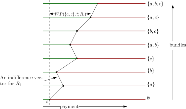
Figure 1: Representation of classical preferences

2.2 Domains and mechanisms

A bundle allocation is an ordered sequence of objects $(A_{1},\ldots,A_{n})$, where $A_{i}$ denotes the bundle allocated to agent $i$, such that for each $A_{i},A_{j}\in\mathcal{B}$, we have $A_{i}\cap A_{j}=\emptyset$ - note that $A_{i}$ can be equal to $\emptyset$ for any $i$ in an object allocation. Let $\mathcal{X}$ denote the set of all bundle allocations.

An outcome profile $((A_{1},t_{1}),\ldots,(A_{n},t_{n}))$ is a collection of $n$ outcomes such that $(A_{1},\ldots,A_{n})$ is the bundle allocation and $t_{i}$ denotes the payment made by agent $i$. An outcome profile $((A_{1},t_{1}),\ldots,(A_{n},t_{n}))$ is Pareto efficient at $R\equiv(R_{1},\ldots,R_{n})$, if there does not exist another outcome profile $((A^{\prime}_{1},t^{\prime}_{1}),\ldots,(A^{\prime}_{n},t^{\prime}_{n}))$ such that

1. for each $i\in N,(A_{i}^{\prime},t_{i}^{\prime})~{}R_{i}~{}(A_{i},t_{i})$,

2. $\sum_{i\in N}t_{i}^{\prime}\geq\sum_{i\in N}t_{i}$,

with one of the inequalities strictly satisfied. The first relation says that each agent $i$ prefers $(A^{\prime}_{i},t^{\prime}_{i})$ to $(A_{i},t_{i})$. The second relation requires that the seller is not spending money to make everyone better off. Without the second relation, we can always improve any outcome profile by subsidizing the agents.

A domain or type space is any subset of classical preferences. A typical domain of preferences will be denoted by $\mathcal{T}$. A mechanism is a pair $(f,\mathbf{p})$, where $f:\mathcal{T}^{n}\rightarrow\mathcal{X}$ and $\mathbf{p}\equiv(p_{1},\ldots,p_{n})$ is a collection of payment rules with each $p_{i}:\mathcal{T}^{n}\rightarrow\mathbb{R}$. Here, $f$ is the bundle allocation rule and $p_{i}$ is the payment rule of agent $i$. We denote the bundle allocated to agent $i$ at type profile $R$ by $f_{i}(R)\in\mathcal{B}$ in the bundle allocation rule $f$.

We require the following properties from a mechanism, which we term desirable.

Definition 2 (Desirable mechanisms)

A mechanism $(f,\mathbf{p})$ is desirable if

1. it is dominant strategy incentive compatible (DSIC): for all $i\in N$, for all $R_{-i}\in\mathcal{T}^{n-1}$, and for all $R_{i},R^{\prime}_{i}\in\mathcal{T}$, we have

   $$\Big{(}f_{i}(R),p_{i}(R)\Big{)}~{}R_{i}~{}\Big{(}f_{i}(R_{i}^{\prime},R_{-i}),p_{i}(R^{\prime}_{i},R_{-i})\Big{)}.$$

2. it is Pareto efficient: $\Big{(}(f_{1}(R),p_{1}(R)),\ldots,(f_{n}(R),p_{n}(R))\Big{)}$ is Pareto efficient at $R$, for all $R\in\mathcal{T}^{n}$.

3. it is individually rational (IR): for all $R\in\mathcal{T}^{n}$ and for all $i\in N$,

   $$\Big{(}f_{i}(R),p_{i}(R)\Big{)}~{}R_{i}~{}(\emptyset,0).$$

4. satisfies no subsidy: for all $R\in\mathcal{T}^{n}$ and for all $i\in N$,

   $$p_{i}(R)\geq 0.$$

We will explore domains where a desirable mechanism exists. DSIC, Pareto efficiency, and IR are standard constraints in mechanism design. No subsidy is debatable. Our motivation for considering it as desirable stems from the fact that most auction formats in practice and the VCG mechanism satisfy it. It also discourages fake buyers from participating in the mechanism.

2.3 A motivating example

In this section, we provide an example to give some intuition for one of our main results.

Example 1

Consider a setting with three agents $N=\{1,2,3\}$, and two objects $M=\{a,b\}$. We are interested in a preference profile where agents 2 and 3 have identical preference: $R_{2}=R_{3}=R_{0}$. In particular, all non-empty bundles have the same willingness to pay according to $R_{0}$ and satisfy

$$WP(\{a,b\},t;R_{0})=WP(\{a\},t;R_{0})=WP(\{b\},t;R_{0})=2+3t,$$

for $t>-\frac{1}{2}$. We are silent about the willingness to pay below $-\frac{1}{2}$, but it can be taken to be $0.5$. We will only consider payments $t>-\frac{1}{2}$ for this example. At preference $R_{0}$, we have

$$(\{a,b\},2+4t)~{}I_{0}~{}(\{b\},2+4t)~{}I_{0}~{}(\{a\},2+4t)~{}I_{0}~{}(\emptyset,t),$$

for all $t>-\frac{1}{2}$. Hence, as $t$ increases, bundle $\{a\}$ (or $\{b\}$ or $\{a,b\}$) will require more payment to be indifferent to $(\emptyset,t)$. We term this negative income effect.

	$\{a\}$	$\{b\}$	$\{a,b\}$
$WP(\cdot,0;R_{1})$	$0$	$0$	$3.9$
$WP(\cdot,0;R_{2}=R_{0})$	$2$	$2$	$2$
$WP(\cdot,0;R_{3}=R_{0})$	$2$	$2$	$2$

Table 1: A profiles of preferences with $M=\{a,b\}$, $N=\{1,2,3\}$.

Agent $1$ has quasilinear preference with a value of $3.9$ for bundle $\{a,b\}$; value zero (or, arbitrarily close to zero) for bundle $\{a\}$ and bundle $\{b\}$, and value of bundle $\emptyset$ is normalized to zero. We denote this preference as $R_{1}$. The willingness to pay at zero payment for these preferences are shown in Table 1.

Suppose $(f,\mathbf{p})$ is a desirable mechanism defined on a (rich enough) type space $\mathcal{T}$ containing the preference profile $R\equiv(R_{1},R_{2}=R_{0},R_{3}=R_{0})$. Notice that the value of $\{a,b\}$ for agent $1$ is 3.9 but $WP(\{a\},0;R_{2})+WP(\{b\},0;R_{3})=4$. Hence, a consequence of Pareto efficiency, individual rationality, and no subsidy is that $f_{1}(R)=\emptyset$. Then, without loss of generality, agent $2$ gets bundle $\{a\}$ and agent $3$ gets bundle $\{b\}$ due to Pareto efficiency.

Next, we can pin down the payments of agents at $R$. Since agent $1$ gets $\emptyset$, her payment must be zero by IR and no subsidy. Now, pretend as if agents $2$ and $3$ have quasilinear preference with valuations equal to their willingness to pay at zero payment (see Table 1). Then, the VCG mechanism would charge them their externalities, which is equal to $1.9$ for both the agents. If the type space $\mathcal{T}$ is sufficiently rich (in a sense, we make precise later), DSIC will still require that $p_{2}(R)=p_{3}(R)=1.9$ (a precise argument is given in the proof of Theorem 1).

The negative income effect of $R_{0}$ makes the Pareto improvement possible in this example. The maximum payment we can extract from agent $1$ is $3.9$. Hence, to collect more payment than the VCG outcome, we can pay a maximum of $0.1(=3.9-3.8)$ to agents 2 and 3. If the preference $R_{0}$ was quasilinear, agents 2 and 3 would have required a compensation of $0.1$ each to be indifferent between not getting any objects and the VCG outcome. Due to negative income effect, agents 2 and 3 can be made to improve from their VCG outcome by paying them much lower amounts. This in turn enables us to Pareto dominate the VCG outcome.

To be precise, the following outcome vector Pareto dominates the outcome of the mechanism at $R$:

$$z_{1}:=(\{a,b\},3.9),~{}~{}z_{2}:=(\emptyset,-0.025),~{}~{}z_{3}:=(\emptyset,-0.025).$$

To see why, note that (a) sum of payments in $z$ is $3.85>p_{2}(R)+p_{3}(R)=3.8$; (b) agent $1$ is indifferent between $z_{1}$ and $(\emptyset,0)$; (c) agents 2 and 3 are also indifferent between their outcomes in the mechanism and $z$ since $(\emptyset,-0.025)~{}I_{0}~{}(\{a\},1.9)$ (because $WP(\{a\},t;R_{0})=2+3t$ for all $t>-0.5$).

It is important to note that $R_{1}$ having high value on $\{a,b\}$ and (almost) zero value on all other bundles played a crucial role in determining payments of agents, and hence, in the impossibility. Indeed, if agent $1$ also had equal willingness to pay on some smaller bundle, then the example will not work. This motivates the class of preferences we study in the next section. $\lozenge$

2.4 Dichotomous preferences

We turn our focus on a subset of classical preferences which we call dichotomous. The dichotomous preferences can be described by: (a) a collection of bundles, which we call the acceptable bundles, and (b) a willingness to pay function, which only depends on the payment level. Formally, it is defined as follows.

Definition 3

A classical preference $R_{i}$ of agent $i$ is dichotomous if there exists a non-empty set of bundles $\emptyset\neq\mathcal{S}_{i}\subseteq(\mathcal{B}\setminus\{\emptyset\})$ and a willingness to pay (WP) map $w_{i}:\mathbb{R}\rightarrow\mathbb{R}_{++}$ such that for every $t\in\mathbb{R}$,

$$WP(A,t;R_{i})=\left\{\begin{array}[]{l l}w_{i}(t)&\forall~{}A\in\mathcal{S}_{i}\\ 0&\forall~{}A\in\mathcal{B}\setminus\mathcal{S}_{i}.\end{array}\right.$$

In this case, we refer to $\mathcal{S}_{i}$ as the collection of acceptable bundles.

The interpretation of the dichotomous preference is that, given same price (payment) for all the bundles, the agent is indifferent between the bundles in $\mathcal{S}_{i}$. Similarly, she is indifferent between the bundles in $\mathcal{B}\setminus\mathcal{S}_{i}$, but it strictly prefers a bundle in $\mathcal{S}_{i}$ to a bundle outside it. Hence, a dichotomous preference can be succinctly represented by a pair $(w_{i},\mathcal{S}_{i})$, where $w_{i}:\mathbb{R}\rightarrow\mathbb{R}_{++}$ is a WP map and $\emptyset\neq\mathcal{S}_{i}\subseteq(\mathcal{B}\setminus\{\emptyset\})$ is the set of acceptable bundles.

By our monotonicity requirement (free-disposal) of classical preference, for every $S,T\in\mathcal{B}$, we have

$$\Big{[}S\subseteq T,S\in\mathcal{S}_{i}\Big{]}\Rightarrow\Big{[}T\in\mathcal{S}_{i}\Big{]}.$$

Hence, a dichotomous preference can be described by $w_{i}$ and a minimal set of bundles $\mathcal{S}^{min}_{i}$ such that

$$\mathcal{S}_{i}:=\{T\in\mathcal{B}:S\subseteq T~{}\textrm{for some}~{}S\in\mathcal{S}^{min}_{i}\}.$$

Figure 2 shows two indifference vectors of a dichotomous preference. The figure shows that the bundles $\{a\},\{a,c\},\{a,b\}$ and $\{a,b,c\}$ are acceptable but others are not.

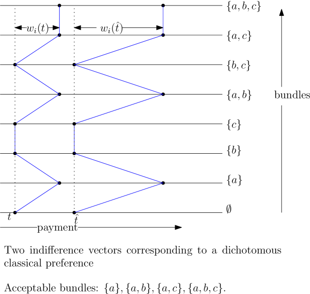
Figure 2: A dichotomous preference

We will denote the domain of all dichotomous preferences as $\mathcal{D}$, where each preference in $\mathcal{D}$ for agent $i$ is described by a $w_{i}$ map and a collection of minimal bundles $\mathcal{S}^{min}_{i}$. A dichotomous domain is any subset of dichotomous preferences.

For some of our results, we will need a particular type of dichotomous preference.

Definition 4

A dichotmous preference $R_{i}\equiv(\mathcal{S}_{i}^{min},w_{i})$ is called a single-minded preference if $|\mathcal{S}_{i}^{min}|=1$.

An agent having a single-minded dichotomous preference has a unique bundle of objects and all its supersets as acceptable bundles. Let $\mathcal{D}^{single}$ denote the set of all single-minded preferences. Single-minded preferences are well-studied in the algorithmic game theory literature (Lehmann et al., 2002; Babaioff et al., 2005, 2009). They were also central in the recent analysis of US incentive auction (Milgrom and Segal, 2020). Our main negative result will be for domains containing $\mathcal{D}^{single}$. Establishing a negative result on domains containing $\mathcal{D}^{single}$ implies a negative result on domains containing $\mathcal{D}$ since $\mathcal{D}^{single}\subsetneq\mathcal{D}$.

Before concluding this section, we briefly discuss how dichotomous preferences are similar to some other kinds of preferences in the literature. In the single object model, the preferences are clearly dichotomous, where there is no uncertainty about the acceptable bundles. Similarly, consider the unit demand preferences studied in Demange and Gale (1985); Morimoto and Serizawa (2015). A preference $R_{i}$ is a unit demand preference if for every $S\in\mathcal{B}$ and every $t\in\mathbb{R}$, we have $WP(S,t;R_{i})=\max_{a\in S}WP(\{a\},t;R_{i})$. Now, suppose the objects are homogeneous in the following sense: $WP(\{a\},t;R_{i})=WP(\{b\},t;R_{i})$ for all $a,b\in M$ and for all $t\in\mathbb{R}$. It is clear that a unit demand preference $R_{i}$ over homogeneous objects is a dichotomous preference, where $\mathcal{S}^{min}_{i}$ consists of singleton bundles. If the objects are not homogeneous, the unit demand preferences are not dichotmous since the willingness to pay of different objects may be different.

3 The results

We describe our main results in this section.

3.1 An impossibility result

We start with our main negative result: if the domain consists of all single-minded preferences, then there is no desirable mechanism. This generalizes the intuition we demonstrated in the example in Section 2.3.

Theorem 1 (Impossibility)

Suppose $\mathcal{T}\supseteq\mathcal{D}^{single}$ (i.e., the domain contains all single-minded preferences), $n\geq 3$, and $m\geq 2$. Then, no desirable mechanism exists in $\mathcal{T}^{n}$.

The proof of this theorem and all other proofs are relegated to an appendix at the end. The proof formalizes the sketch given in the example in Section 2.3. The main idea of the proof is that if a desirable mechanism exists in $\mathcal{D}^{single}$, it has to define outcomes at all single-minded preference profiles, which includes an $n$-agent and $m$-object version of the preference profile discussed in Section 2.3. The challenge is to show that any desirable mechanism at that profile must coincide with the outcome of a generalized VCG mechanism (where agents pay their “externalities"). Once this is shown, the rest of the proof is similar to the discussion in Section 2.3.

As discussed in the introduction, Theorem 1 adds to a small list of papers that have established such negative results in other combinatorial auction problems. Notice that the domain $\mathcal{T}$ may contain preferences that are not dichotomous or it may be equal to $\mathcal{D}$, the set of all dichotomous preferences.

The conditions $m\geq 2$ and $n\geq 3$ are both necessary: if $m=1$, we know that a desirable mechanism exists (Saitoh and Serizawa, 2008); if $n=2$, the mechanism that we propose next is desirable – see Proposition 1 and discussions after it.

Definition 5

The generalized Vickrey-Clarke-Groves mechanism with loser’s payment $t_{L}$ (GVCG-$t_{L}$), denoted as $(f^{vcg,t_{L}},\mathbf{p}^{vcg,t_{L}})$, is defined as follows: for every profile of preferences $R$,

$$f^{vcg,t_{L}}(R) \in\arg\max_{A\in\mathcal{X}}\sum_{i\in N}WP(A_{i},t_{L};R_{i})$$

$$p^{vcg,t_{L}}_{i}(R) =t_{L}+\max_{A\in\mathcal{X}}\sum_{j\neq i}WP(A_{j},t_{L};R_{j})-\sum_{j\neq i}WP(f^{vcg,t_{L}}_{j}(R),t_{L};R_{j}).$$

We refer to the GVCG-$0$ mechanism as the GVCG mechanism.

The GVCG class of mechanisms is a natural generalization of the VCG mechanism to our setting without quasilinearity. Note that the current definition does not use anything about dichotomous preferences. It computes the “externality” of every agent with respect to a reference transfer level $t_{L}$. This transfer level $t_{L}$ corresponds to the payment by any agent who does not win any non-empty bundle of objects in the mechanism (such an agent has zero externality). The additional term $t_{L}$ in the payment expression ensures that when we use $t_{L}$ as the reference transfer level to compute externalities, we maintain incentive compatibility in the dichotomous domain. In the quasilinear domain, the reference transfer level does not matter as the willingness to pay does not change with reference transfer: $WP(S,t_{L},R_{i})=WP(S,0,R_{i})$ for each $S$, if $R_{i}$ is a quasilinear preference.

Theorem 1 implies that the GVCG mechanism is not desirable. Indeed, no GVCG mechanism can be DSIC in an arbitrary combinatorial auction domain without quasilinearity. For instance, Morimoto and Serizawa (2015) show that there is a unique desirable mechanism in the domain of “unit-demand" (where agents have demand for at most one object) preferences, and it is not a GVCG mechanism. We show that the GVCG mechanism is DSIC, individually rational, and satisfies no subsidy in any dichotomous preference domain.

Proposition 1

Consider the GVCG-$t_{L}$ mechanism for some $t_{L}\in\mathbb{R}$, defined on an arbitrary dichotomous domain $\mathcal{T}\subseteq\mathcal{D}$. Then, the following are true.

1. The GVCG-$t_{L}$ mechanism is DSIC.

2. The GVCG-$t_{L}$ mechanism is individually rational if $t_{L}\leq 0$.

3. The GVCG-$t_{L}$ mechanism satisfies individual rationality and no subsidy if $t_{L}=0$.

4. The GVCG-$t_{L}$ mechanism is Pareto efficient if $n=2$.

5. The GVCG-$t_{L}$ mechanism is not Pareto efficient if $n>2,m>1$, and $\mathcal{T}\supseteq\mathcal{D}^{single}$.

We explain below why the GVCG class of mechanisms are compatible with Pareto efficiency when $n=2$ but not compatible when $n>2$. For simplicity, we assume that preferences of agents are single-minded, i.e., the domain is $\mathcal{D}^{single}$. We consider various cases.

One object ($m=1$). It is well known that the GVCG mechanism is Pareto efficient if $m=1$ (Saitoh and Serizawa, 2008). Note that for $m=1$, every preference is single-minded. The GVCG mechanism allocates the object to an agent $k$ with the highest WP at $0$, i.e., $w_{k}(0)=\max_{i\in N}w_{i}(0)$. All agents except agent $k$ pay zero and agent $k$ pays $\max_{i\neq k}w_{i}(0)$. This outcome is always Pareto efficient. The main reason for this is that there is only one object, and any new outcome can only give this object to one agent (may be the same or another agent). Take any such outcome $z\equiv(z_{1},\ldots,z_{n})$ and assume for contradiction that it Pareto dominates the GVCG outcome. If agent $k$ continues to get the object in $z_{k}$ also, her payment cannot be more than $\max_{i\neq k}w_{i}(0)$. Further, payments of other agents cannot be more than zero. As a result, total payment cannot be more than $\max_{i\neq k}w_{i}(0)$. Similarly, if any other agent $j\neq k$ receives the object in $z$, then her payment cannot be more than $w_{j}(0)$ (else, she will prefer the GVCG outcome of getting nothing and paying zero). Further, in this case, since agent $k$ does not receive the object in $z$, her payment will be non-positive. As a result, the total payment cannot be more than $\max_{i\neq k}w_{i}(0)$. In fact, the total payment in $z$ in both the cases will be strictly less than the GVCG payments if any agent strictly improves, which is a contradiction.

Two agents ($n=2$) but arbitrary $m$. Since preferences of agents are single-minded, at every preference profile the acceptable bundles of each agent $i$ are supersets of some $S_{i}\in\mathcal{B}$. Since there are two agents, we have only two cases to consider: (i) $S_{1}\cap S_{2}=\emptyset$ and (ii) $S_{1}\cap S_{2}\neq\emptyset$. Intuitively, in the first case, the two agents are not competing against each other. Pareto efficiency requires us to allocate each agent $i\in\{1,2\}$ her acceptable bundle $S_{i}$. The GVCG mechanism charges zero payment to the agents. Clearly, this cannot be Pareto dominated. In the second case, the two agents compete against each other like the single object case. This is because $S_{1}\cap S_{2}\neq\emptyset$ means exactly one agent can be assigned an acceptable bundle. In fact the allocation and payment in the GVCG mechanism for this case mirrors the single object case: the agent with the higher WP at $0$ gets her acceptable bundle and pays the willingness to pay of the other agent. The fact that this outcome cannot be Pareto dominated follows an argument similar to the $m=1$ case. Summarizing, if there are two agents, independent of the number of objects, the Pareto efficiency requirement is very similar to the single object case. Hence, the GVCG mechanism remains compatible with Pareto efficiency.

More than two agents and more than one object ($n>2,m>1$). With more than two agents and more than one object, the Pareto efficiency requirement is no longer like the single object case. To understand, let us consider Example 1 (see Table 1). The GVCG mechanism allocates objects $a$ and $b$ to agents $2$ and $3$ but charges them low payments ($1.9$ each). This is akin to low payments in the VCG mechanism as documented in Ausubel and Milgrom (2006). In our example, even though agent $1$ is not allocated any object, she has high enough willingness to pay for the bundle of objects – with one object, if the payment of the winning agent is low, then the willingness to pay of all losing agents is also low. With negative income effect, agents $2$ and $3$ feel “wealthier" after getting the objects at low payments. So, their “willingness to sell" amount is low. Hence, it is easier to compensate them. With agent $1$ having a high enough willingness to pay ($3.9$), a Pareto improving trade is thus possible. Such a Pareto improving trade is not possible if agents $2$ and $3$ have positive income effect preferences. This is because with positive income effect, the “willingness to sell" amount is higher than the willingness to pay.

3.2 Positive income effect and possibility

Proposition 1 and Theorem 1 point out that the GVCG is not Pareto efficient in the entire dichotomous domain. A closer look at the proof of Theorem 1 (and Example 1) reveals that the impossibility is driven by a particular kind of dichotomous preferences: the ones where the willingness to pay of an agent increases with payment. We term such preferences negative income effect.

A standard definition of positive income effect will say that as income rises, a preferred bundle becomes “more preferred". We do not model income explicitly, but our preferences implicitly account for income. So, if payment decreases from $t$ to $t^{\prime}$, the income level of the agent increases implicitly. As a result, she is willing to pay more for his acceptable bundles at $t^{\prime}$ than at $t$. Thus, positive income effect captures a reasonable (and standard) restriction on preferences of the agents.

Definition 6

A dichotomous preference $R_{i}\equiv(w_{i},\mathcal{S}_{i})$ satisfies positive income effect if for all $t>t^{\prime}$, we have $w_{i}(t)\leq w_{i}(t^{\prime}).$

A dichotomous domain of preferences $\mathcal{T}$ satisfies positive income effect if every preference in $\mathcal{T}$ satisfies positive income effect.

As an illustration, the indifference vectors shown in Figure 2 cannot be part of a dichotomous preference satisfying positive income effect – we see that $\hat{t}>t$ but $w_{i}(\hat{t})>w_{i}(t)$. The preference $R_{0}$ in Example 1 also violated positive income effect. A quasilinear preference (where $w_{i}(t)=w_{i}(t^{\prime})$ for all $t,t^{\prime}$) always satisfies positive income effect, and the GVCG mechanism is known to be a desirable mechanism in this domain. We show below that the GVCG mechanism is Pareto efficient if the domain contains preferences that satisfy positive income effect. Before stating the result, let us reconsider Example 1 and see why the GVCG mechanism becomes desirable with positive income effect.

Example 2

We revisit Example 1 but with an important difference: the preferences of agents 2 and 3 now satisfy positive income effect. So, we have three agents $N=\{1,2,3\}$ and two objects $M=\{a,b\}$. As in Example 1, agent $1$ has single-minded quasilinear preference $R_{1}$ with valuation $3.9$ on the unique acceptable bundle $\{a,b\}$. All the bundles are acceptable bundles for agents 2 and 3. But their preference is now $\widehat{R}_{0}$ which satisfies positive income effect. However, similar to Example 1, we have $\widehat{w}(0)=2$. Figure 3 shows two indifference vectors of $\widehat{R}_{0}$. Since $\widehat{R}_{0}$ satisfies positive income effect, we have $\widehat{w}(t)>\widehat{w}(0)$, where $t<0$.

The GVCG outcome does not change from Example 1 at this profile: agent $2$ gets object $a$ and agent $3$ gets object $b$ with payments $p_{1}^{vcg}=0,p_{2}^{vcg}=p_{3}^{vcg}=1.9$. To Pareto dominate this outcome, we need to give both the objects to agent $1$.

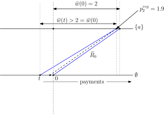
Figure 3: Possibility with positive income effect

	$\{a\}$	$\{b\}$	$\{a,b\}$
$WP(\cdot,0;R_{1})$	$0$	$0$	$3.9$
$WP(\cdot,0;R_{2}=\widehat{R}_{0})$	$2$	$2$	$2$
$WP(\cdot,0;R_{3}=\widehat{R}_{0})$	$2$	$2$	$2$

Table 2: A profiles of preferences with $M=\{a,b\}$, $N=\{1,2,3\}$.

Now, the GVCG outcome to agent $2$ is $(\{a\},1.9)$ and, by Table 2 (see Figure 3 also), $(\{a\},2)~{}\widehat{I}_{0}~{}(\emptyset,0)$. If $(\{a\},1.9)~{}\widehat{I}_{0}~{}(\emptyset,t)$, then by positive income effect $t<-0.1$. A pictorial description of the indifference vectors of $\widehat{R}_{0}$ for these transfer amounts are shown in Figure 3. This means that if agent $2$ is not given any object, the total compensation required for her alone will be more than $0.1$. Since agent $3$ needs to be compensated too and the total revenue collected in the VCG outcome is $3.8$, we need to charge more than $3.9$ to agent $1$ to Pareto dominate the VCG outcome. This is impossible since the value of agent $1$ for both the objects is only $3.9$. $\lozenge$

The intuition in this example generalizes. The main idea is that the GVCG mechanism allocates goods in a way that maximizes the collective willingness to pays (at zero) of the winning bidders. IR implies that the winning bidders pay a price less than their willingness to pay for their winning bundles. Thus, winning essentially makes the bidders feel “wealthier". Positive income effect then implies that their “willingness to sell" after the auction exceeds the willingness to pay before the auction. This rules out any Pareto improving trades.

Our next result says that the impossibility in Theorem 1 is overturned in any domain of dichotomous preferences satisfying positive income effect.

Theorem 2 (Possibility)

The GVCG mechanism is desirable on any dichotomous domain satisfying positive income effect.

Theorem 2 can be interpreted to be a generalization of the well-known result that the VCG mechanism is desirable in the quasilinear domain. Indeed, we know that if the domain of preferences is the set of all quasilinear preferences, then standard revenue equivalence result (which holds in the quasilinear domain) implies that the VCG mechanism is the only desirable mechanism. Though we do not have a revenue equivalence result, we show below a similar uniqueness result of the GVCG mechanism. For this, we first remind ourselves of the definition of a quasilinear preference. A dichotomous preference $(w_{i},\mathcal{S}_{i})$ is quasilinear if for every $t,t^{\prime}\in\mathbb{R}$, we have $w_{i}(t)=w_{i}(t^{\prime})$. We denote by $\mathcal{D}^{QL}$ the set of all dichotomous quasilinear preferences. This leads to a characterization of the GVCG mechanism.

Theorem 3 (Uniqueness)

Suppose the domain of preferences $\mathcal{T}$ is a dichotomous domain satisfying positive income effect and contains $\mathcal{D}^{QL}$. Let $(f,\mathbf{p})$ be a mechanism defined on $\mathcal{T}^{n}$. Then, the following statements are equivalent.

1. $(f,\mathbf{p})$ is a desirable mechanism.

2. $(f,\mathbf{p})$ is the GVCG mechanism.

We reiterate that the GVCG is known to fail DSIC with non-quasilinear preferences if agents demand multiple objects. So, Theorems 2 and 3 show that under dichotomous classical preferences with positive income effect, we recover the desirability of the GVCG mechanism.

3.3 Tightness of results

In this section, we investigate if the positive results in the previous sections continue to hold if the domain includes (positive income effect) non-dichotomous preferences. In particular, we investigate the consequences of adding a non-dichotomous preference satisfying positive income effect and some other reasonable properties (we precisely define them later in the section). Both these conditions are natural properties to impose on preferences. Our results below can be summarized as follows: if we take the set of all quasilinear dichotomous preferences and add any non-dichotomous preference satisfying the above two conditions, then no desirable mechanism can exist in such a type space. As corollaries, we uncover new type spaces where no desirable mechanism can exist with non-quasilinear preferences, and establish the role of dichotomous preferences in such type spaces. Before we formally state the result, we give an example to show why we should expect such an impossibility result.

	$\{a\}$	$\{b\}$	$\{a,b\}$
$WP(\cdot,0;R_{1})$	$0$	$0$	$5$
$WP(\cdot,0;R_{2}=R_{0})$	$3$	$4$	$4$
$WP(\cdot,0;R_{3}=R_{0})$	$3$	$4$	$4$
$WP(\cdot,0;R^{\prime}_{2})$	$0$	$4$	$4$

Table 3: Two profiles of preferences with $M=\{a,b\}$, $N=\{1,2,3\}$.

Example 3

We consider an example with two object $M:=\{a,b\}$ and three agents $N:=\{1,2,3\}$. We will require the following preferences of the agents. The preference $R_{1}$ of agent $1$ is quasilinear and the corresponding values for bundles of objects is shown in Table 3. It is clear that $R_{1}$ is a single-minded preference. We have two preferences of agent $2$: $R_{2}=R_{0}$ and $R^{\prime}_{2}$. Preference $R_{0}$ is not quasilinear, but it satisfies positive income effect (decreasing prices by the same amount of two indifferent consumption bundles lead the agents to strictly prefer the costlier object): $(\{b\},4)~{}I_{0}~{}(\{a\},3)$ and $(\{b\},2)~{}P_{0}~{}(\{a\},1)$. This is shown in Figure 4, where we show some indifference vectors of $R_{0}$. Note that the other indifference vectors of $R_{0}$ can be constructed such that it satisfies the unit demand property and positive income effect. Preference $R^{\prime}_{2}$ is a quasilinear single-minded preference with $\{b\}$ and $\{a,b\}$ as acceptable bundles and value $4$. Finally, preference $R_{3}$ of agent $3$ is also $R_{0}$.

Figure 4: Positive income effect preference of agents $2$ and $3$.

We argue that the GVCG mechanism containing all quasilinear dichotomous preferences and $R_{0}$ is not DSIC. So, our domain is $\mathcal{T}=\mathcal{D}^{QL}\cup\{R_{0}\}$. We will look at two preference profiles: $(R_{1},R_{2},R_{3})$ and $(R_{1},R^{\prime}_{2},R_{3})$. At the preference profile $(R_{1},R_{2},R_{3})$, agents 2 and 3 should get objects from $\{a,b\}$ according to GVCG. Since they have identical preferences, we break the tie by giving object $a$ to agent $2$ and object $b$ to agent $3$: $f_{1}^{vcg}(R_{1},R_{2},R_{3})=\{a\},f^{vcg}_{2}(R_{1},R_{2},R_{3})=\{b\}$. The payment of agent $2$ is $p^{vcg}_{2}(R_{1},R_{2},R_{3})=1$.

Now, consider the preference profile $(R_{1},R^{\prime}_{2},R_{3})$. Here, since agent $2$ has only $\{b\}$ and $\{a,b\}$ in her acceptable bundle, her GVCG outcome changes: $f_{2}^{vcg}(R_{1},R^{\prime}_{2},R_{3})=\{b\}$ and $p_{2}^{vcg}(R_{1},R^{\prime}_{2},R_{3})=2$. In other words, the externality of agent $2$ changes from $1$ at preference profile $(R_{1},R_{2},R_{3})$ to $2$ at $(R_{1},R^{\prime}_{2},R_{3})$.

If $R_{2}$ was a quasilinear preference, then agent $2$ would have been indifferent between $(\{a\},1)$ and $(\{b\},2)$. But since $R_{2}=R_{0}$ satisfies positive income effect (see Figure 4), $(\{b\},2)~{}P_{2}~{}(\{a\},1)$. This shows that with positive income effect, agent $2$ can manipulate in the GVCG mechanism in this domain.

This is a general problem. We formalize this in Theorem 4. We show in the proof of Theorem 4 that any desirable mechanism in such a domain must have the GVCG outcomes at these profiles, and this will lead to manipulation by the agent having positive income effect.

It is crucial that $WP(\{a\},0;R_{0})<WP(\{b\},0;R_{0})$ for this manipulation to happen in this example. If $WP(\{a\},0;R_{0})=WP(\{b\},0;R_{0})=4$, then $R_{0}$ can be a dichotomous preference (i.e., besides the indifference vector shown in Table 3, we can construct other indifference vectors such that it is a dichotomous preference). We know that the GVCG mechanism is DSIC in such domains. Indeed, in that case, the externality of agent $2$ remains unchanged across profiles $(R_{1},R_{2},R_{3})$ and $(R_{1},R^{\prime}_{2},R_{3})$. In other words, we have $p^{vcg}_{2}(R_{1},R_{2},R_{3})=p^{vcg}_{2}(R_{1},R^{\prime}_{2},R_{3})=1$. So, no manipulation is possible by agent $2$ across these two preference profiles.

$\lozenge$

We formalize the intuition in Example 3 now. We consider a preference where an agent can demand multiple heterogeneous objects. We require that at least two objects are heterogeneous in the following sense.

Definition 7

A preference $R_{i}$ satisfies heterogenous demand if there exists $a,b\in M$,

$$WP(\{a\},0;R_{i})\neq WP(\{b\},0;R_{i}).$$

Heterogeneous demand requires that for some pair of objects, the WP at $0$ must be different for them. If objects are not the same (i.e., not homogeneous), then we should expect this condition to hold. We can provide an analogous tightness result if objects are homogeneous.

Besides the heterogeneous demand, we will impose two natural conditions on preferences. The first condition is a mild form of substitutability condition.

Definition 8

A preference $R_{i}$ satisfies strict decreasing marginal WP if for every $a,b\in M$,

$$WP(\{a\},0;R_{i})+WP(\{b\},0;R_{i})>WP(\{a,b\},0;R_{i}).$$

Strict decreasing marginal WP requires a minimal degree of submodularity: the marginal increase in WP (at $0$) by adding $\{a\}$ to $\{b\}$ is less than adding $\{a\}$ to $\emptyset$. Notice that this substitutability requirement is only for bundles of size two. Hence, larger bundles may exhibit complementarity or substitutability. Because of free disposal, for every $a,b\in M$, we have

$$WP(\{a,b\},0;R_{i})\geq\max(WP(\{a\},0;R_{i}),WP(\{b\},0;R_{i})).$$

Hence, strict decreasing marginal WP implies that $WP(\{a\},0;R_{i})>0$ and $WP(\{b\},0;R_{i})>0$, i.e., each object is a good in a weak sense (getting an object is preferred to getting nothing at payment $0$).

We point out that unit demand preferences (studied in (Demange and Gale, 1985; Morimoto and Serizawa, 2015)) satisfy strict decreasing marginal WP. A preference $R_{i}$ is called a unit demand preference if for every $S$,

$$WP(S,t;R_{i})=\max_{a\in S}WP(\{a\},t;R_{i})~{}\forall~{}t\in\mathbb{R}_{+}.$$

If $R_{i}$ is a unit demand preference and objects are goods, then it satisfies strict decreasing marginal WP. To see this, call every object $a\in M$ a real good if $WP(\{a\},0;R_{i})>0$ at every $R_{i}$. If every object is a real good, then for every $a,b\in M$, we see that

$$WP(\{a\},0;R_{i})+WP(\{b\},0;R_{i})>\max_{x\in\{a,b\}}WP(\{x\},0;R_{i})=WP(\{a,b\},0;R_{i}).$$

Besides the strict decreasing marginal WP condition, we will also be requiring strict positive income effect, but only for singleton bundles.

Definition 9

A classical preference $R_{i}$ satisfies strict positive income effect if for every $a,b\in M$ and for every $t,t^{\prime}$ with $t^{\prime}>t$, the following holds for every $\delta>0$:

$$\Big{[}(\{b\},t^{\prime})~{}I_{i}~{}(\{a\},t)\Big{]}~{}\Rightarrow~{}\Big{[}(\{b\},t^{\prime}-\delta)~{}P_{i}~{}(\{a\},t-\delta)\Big{]}.$$

This definition of strict positive income effect requires that if two objects are indifferent then decreasing their prices by the same amount makes the higher priced (lower income) object better. This is a generalization of the definition of positive income effect we had introduced for dichotomous preferences in Definition 6, but only restricted to singleton bundles. This means that for larger bundles, we do not require positive income effect to hold.

We are ready to state the main tightness result with heterogeneous objects.

Theorem 4

Suppose $n\geq 4,m\geq 2$. Let $R_{0}$ be a heterogeneous demand preference satisfying strict positive income effect and strict decreasing marginal WP. Consider any domain $\mathcal{T}$ containing $\mathcal{D}^{QL}\cup\{R_{0}\}$. Then, no desirable mechanism exists in $\mathcal{T}^{n}$.

We make a quick remark about the statement of Theorem 4.

Remark 1.  Though Theorem 4 requires $n\geq 4$, a careful look at its proof reveals that we only need $n\geq 4$ if $m>2$. If there are only two objects, the impossibility result in Theorem 4 holds with $n\geq 3$. This was shown in Example 3 also.

The basic idea of the proof of Theorem 4 is similar to Example 3. With more than two object ($m>2$), we will need at least four agents. The reason is slightly delicate. Notice that $R_{0}$ in the statement of Theorem 4 is an arbitrary preference. As in Example 3, the proof ensures that three agents compete for two objects, say $\{a,b\}$, out of which two agents have $R_{0}$ as their preference. With more than two objects, we need a way to ensure that $\{a,b\}$ are allocated among these three agents. In the absence of a fourth agent, it is not possible to ensure that the two agents having $R_{0}$ preference are not assigned objects outside of $\{a,b\}$. A fourth agent having arbitrarily large willingness to pay for the bundle $M\setminus\{a,b\}$ ensures that.

We do not know if the impossibility result holds for $n=2$ or $n=3$ when $m>2$, but we conjecture that it does not. $\lozenge$

Unlike the negative result in Theorem 1, Theorem 4 does not require the existence of negative income effect dichotomous preferences. It requires the domain to contain the set of quasilinear dichotomous preferences and one heterogeneous demand preference satisfying some reasonable conditions. This negative result parallels a result of Kazumura and Serizawa (2016) who show that adding any multi-demand preference to a class of rich unit demand preference gives rise to a similar impossibility. As was explained in Example 3, our proof exploits the fact that any desirable mechanism must coincide with the GVCG mechanism in the positive income effect dichotomous domain, and adding any strictly positive income effect preference to the domain leads to manipulation. In the case of Kazumura and Serizawa (2016), they add an arbitrary multi-demand preference (which may or may not satisfy positive income effect) to a domain of unit demand preferences, where the GVCG mechanism is not desirable. So, neither of the results imply the other and the proof strategies are different.

We now spell out an exact implication of Theorem 4 in a corollary below. Let $\mathcal{D}^{+}$ be the set of all positive income effect dichotomous preferences (note that $\mathcal{D}^{QL}\subsetneq\mathcal{D}^{+}$) and $\mathcal{U}^{+}$ be the set of all heterogeneous unit demand preferences satisfying positive income effect (as argued earlier, unit demand preferences satisfy strict decreasing marginal WP). Then, the following corollary is immediate from Theorem 4.

Corollary 1

Suppose $\mathcal{T}=\mathcal{D}^{+}\cup\mathcal{U}^{+}$. Then, no desirable mechanism exists on $\mathcal{T}^{n}$.

Theorem 3 shows that the GVCG mechanism is the unique desirable mechanism on $\mathcal{D}^{+}$. Similarly, Demange and Gale (1985) have shown that a desirable mechanism exists in $\mathcal{U}^{+}$. This mechanism is called the minimum Walrasian equilibrium price mechanism and collapses to the VCG mechanism if preferences are quasilinear. Corollary 1 says that we lose these possibility results if we consider the unions of these two type spaces.

4 Related Literature

The quasilinearity assumption is at the heart of mechanism design literature with payments. Our formulation of classical preferences was studied in the context of single object auction by Saitoh and Serizawa (2008), who proposed the generalized VCG mechanism and axiomatized it for that setting. Other such axiomatizations include Sakai (2008, 2013). As discussed, Demange and Gale (1985) had shown that a mechanism different from the generalized VCG mechanism is desirable when multiple heterogeneous objects are sold to agents with unit demand. Characterizations of this mechanism have been given in Morimoto and Serizawa (2015), Zhou and Serizawa (2018) and Kazumura et al. (2020b). However, impossibility results for the existence of a desirable mechanism were shown (a) by Kazumura and Serizawa (2016) for multi-object auctions with multi-demand agents and (b) by Baisa (2020) for multiple homogeneous object model with multi-demand agents. Social choice problems with payments are studied with particular form of non-quasilinear preferences in Ma et al. (2016, 2018). These papers establish dictatorship results in this setting with non-quasilinear preferences.

Baisa (2016) considers non-quasilinear preferences with randomization in a single object auction environment. He proposes a randomized mechanism and establishes strategic properties of this mechanism. Dastidar (2015) considers a model where agents have same utility function but models income explicitly to allow for different incomes. He considers equilibria of standard auctions. Samuelson and Noldeke (2018) discuss an implementation duality without quasilinear preferences and apply it to matching and adverse selection problems. Kazumura et al. (2020a) discuss monotonicity based characterization of DSIC mechanisms in domains which admit non-quasilinear preferences. Baisa and Burkett (2019) discuss a model of single object allocation when bidders have interdependent values and non-quasilinear preferences with positive income effects. They give necessary and sufficient conditions for the existence of an ex-post implementable and Pareto efficient mechanism in two settings: (i) where the auctioneer is the seller; and (ii) the procurement setting, where the auctioneer is the buyer. In the former setting, their condition requires existence of an ex-post implementable and Pareto efficient mechanism in a corresponding quasilinear economy. In the latter setting, they show an impossibility result if the level of interdependence is strong.

The literature on auction design with budget constrained bidders models budget constraint such that if an agent has to pay more than budget, then his utility is minus infinity. This introduces non-quasilinear utility functions but it does not fit our model because of the hard budget constraint. For the multi-unit auction with such budget-constrained agents, Lavi and May (2012) establish that no desirable mechanism can exist – see an extension of this result in Dobzinski et al. (2012). They prove this result by considering two bidders each with publicly known budgets and two units. Their result shows an impossibility similar to ours as long as the public budgets of the bidders are not equal. Their paper also allows complementary preferences but not of the extreme form seen with dichotomous preferences.

For combinatorial auctions with single-minded and quasilinear preferences, Le (2018) shows that these impossibilities with budget-constrained agents can be overcome in a generic sense – he defines a “truncated" VCG mechanism and shows that it is desirable almost everywhere.

There is a literature in algorithmic mechanism design on combinatorial auctions with quasilinear but “single-minded" preferences. Apart from practical significance, the problem is of interest because computing a VCG outcome is computationally challenging but various “approximately" desirable mechanisms which are computationally tractable can be constructed (Babaioff et al., 2005, 2009; Lehmann et al., 2002; Milgrom and Segal, 2020). Rastegari et al. (2011) show that in this model, the revenue from the VCG mechanism (and any DSIC mechanism) may not satisfy monotonicity, i.e., adding an agent may decrease revenue. Our paper adds to this literature by illustrating the implications of non-quasilinear preferences.

Appendix A Proofs

A.1 Proof of Theorem 1

The proof extends the intuition in Example 1.

Proof:  We start by providing two useful lemmas.

Lemma 1

Suppose $(f,\mathbf{p})$ is an individually rational mechanism satisfying no subsidy. Then for every agent $i\in N$ and every $R\in\mathcal{T}^{n}$, we have $p_{i}(R)=0$ if $f_{i}(R)\notin\mathcal{S}_{i}$.

Proof:  Suppose $R$ is a profile such that $f_{i}(R)\notin\mathcal{S}_{i}$ for agent $i$. By individual rationality, $(f_{i}(R),p_{i}(R))~{}R_{i}~{}(\emptyset,0)$. But $f_{i}(R)\notin\mathcal{S}_{i}$ implies that $(\emptyset,p_{i}(R))~{}I_{i}~{}(f_{i}(R),p_{i}(R))~{}R_{i}~{}(\emptyset,0)$. Hence, $p_{i}(R)\leq 0$. But no subsidy implies that $p_{i}(R)=0$. $\blacksquare{}$

Lemma 2

Suppose $(f,\mathbf{p})$ is an individually rational mechanism satisfying no subsidy. Then for every agent $i\in N$ and every $R\in\mathcal{T}^{n}$, we have $0\leq p_{i}(R)\leq WP(f_{i}(R),0;R_{i}).$

Proof:  If $f_{i}(R)\notin\mathcal{S}_{i}$, then the claim follows from Lemma 1. Suppose $f_{i}(R)\in\mathcal{S}_{i}$. By individual rationality, $(f_{i}(R),p_{i}(R))~{}R_{i}~{}(\emptyset,0)~{}I_{i}~{}(f_{i}(R),WP(f_{i}(R),0;R_{i}))$. This implies that $p_{i}(R)\leq WP(f_{i}(R),0;R_{i})$. No subsidy implies that $p_{i}(R)\geq 0$. $\blacksquare{}$

Consider any three non-empty bundles $S,S_{1},S_{2}$ such that $S=S_{1}\cup S_{2}$ and $S_{1}\cap S_{2}=\emptyset$. Consider a profile of single-minded preferences $R^{*}\in\big{(}\mathcal{D}^{single}\big{)}^{n}$ as follows. Since all the agents have dichotomous preferences, to describe any agent $i$’s preference, we describe the minimal acceptable bundles $\mathcal{S}^{min}_{i}$ (i.e., the set of acceptable bundles $\mathcal{S}_{i}$ are derived by taking supersets of each element in $\mathcal{S}^{min}_{i}$) and the willingness to pay map $w_{i}$. Preference $R^{*}_{1}$ of agent $1$ is quasilinear:

$$\mathcal{S}^{min}_{1}=\{S\},w_{1}(t)=3.9~{}\forall~{}t\in\mathbb{R}.$$

Preference $R^{*}_{2}$ of agent $2$ is:

$$\mathcal{S}^{min}_{2}=\{S_{1}\},w_{2}(t)=2+3t~{}\forall~{}t>-\dfrac{1}{2}\textrm{ and }w_{2}(t)=\dfrac{1}{2}\textrm{ otherwise}$$

Preference $R^{*}_{3}$ of agent $3$ is:

$$\mathcal{S}^{min}_{3}=\{S_{2}\},w_{3}(t)=2+3t~{}\forall~{}t>-\dfrac{1}{2}\textrm{ and }w_{3}(t)=\dfrac{1}{2}\textrm{ otherwise}$$

Preference $R^{*}_{i}$ of each agent $i\notin\{1,2,3\}$ is quasilinear:

$$\mathcal{S}^{min}_{i}=\{S\},w_{i}(t)=\epsilon~{}\forall~{}t\in\mathbb{R},$$

where $\epsilon>0$ but very close to zero.

Assume for contradiction that there exists a DSIC, Pareto efficient, individually rational mechanism $(f,\mathbf{p})$ satisfying no subsidy. We now do the proof in several steps.

Step 1. In this step, we show that at every preference profile $R$ with $R_{i}=R^{*}_{i}$ for all $i\notin\{2,3\}$, we must have $S\nsubseteq f_{i}(R)$ if $i\notin\{1,2,3\}$. We know that $\mathcal{S}^{min}_{i}=\{S\}$ for all $i\notin\{2,3\}$. Assume for contradiction $S\subseteq f_{k}(R)$ for some $k\notin\{1,2,3\}$. Then, $S\nsubseteq f_{1}(R)$. By Lemma 1, $p_{1}(R)=0$. Consider the following outcome:

$$Z_{1}=(S,\epsilon),Z_{k}=(\emptyset,p_{k}(R)-\epsilon),Z_{j}=(f_{j}(R),p_{j}(R))~{}\forall~{}j\notin\{1,k\}.$$

Since preferences of agent $1$ and agent $k$ are quasilinear (note that $R_{1}=R^{*}_{1}$ and $R_{k}=R^{*}_{k}$) and $\epsilon$ is very close to zero, we have

$$Z_{1}~{}P_{1}~{}(f_{1}(R),p_{1}(R)=0),Z_{k}~{}I_{k}~{}(f_{k}(R),p_{k}(R)),Z_{j}~{}I_{j}~{}(f_{j}(R),p_{j}(R))~{}\forall~{}j\notin\{1,k\}.$$

Also, the sum of payments in the outcome vector $Z\equiv(Z_{1},\ldots,Z_{n})$ is $\sum_{i\in N}p_{i}(R).$ This contradicts Pareto efficiency of $(f,\mathbf{p})$.

Step 2. Fix a preference $\hat{R}_{2}$ of agent 2 such that $\mathcal{\hat{S}}^{min}_{2}=\{S_{1}\}$ and $\hat{w}_{2}(0)>1.9$. We show that at preference profile $\hat{R}=(\hat{R}_{2},R^{*}_{-2})$, $S\nsubseteq f_{1}(\hat{R})$. Suppose $S\subseteq f_{1}(\hat{R})$. Then, $S_{1}\nsubseteq f_{2}(\hat{R})$ and $S_{2}\nsubseteq f_{3}(\hat{R})$. By Lemma 1, $p_{2}(\hat{R})=0,p_{3}(\hat{R})=0$. Consider a new outcome vector:

$$Z_{1}=(\emptyset,p_{1}(\hat{R})-3.9),Z_{2}=(S_{1},\hat{w}_{2}(0)),Z_{3}=(S_{2},w_{3}(0)),Z_{j}=(f_{j}(\hat{R}),p_{j}(\hat{R}))~{}\forall~{}j\notin\{1,2,3\}.$$

By quasilinearity of $R^{*}_{1}$, we get $Z_{1}~{}I^{*}_{1}~{}(f_{1}(\hat{R}),p_{1}(\hat{R}))$. By definition,

$$Z_{2}~{}\hat{I}_{2}~{}(\emptyset,0)~{}\hat{I}_{2}~{}(f_{2}(\hat{R}),p_{2}(\hat{R})).$$

Similarly, $Z_{3}~{}I^{*}_{3}~{}(f_{3}(\hat{R}),p_{3}(\hat{R}))$. Further, the sum of payments in the outcome vector $Z$ is

$$p_{1}(\hat{R})-3.9+\hat{w}_{2}(0)+w_{3}(0)+\sum_{j\notin\{1,2,3\}}p_{j}(\hat{R})>\sum_{j\in N}p_{j}(\hat{R}),$$

where the inequality used the fact that $p_{2}(\hat{R})=p_{3}(\hat{R})=0$ and $\hat{w}_{2}(0)>1.9,w_{3}(0)=2$. This contradicts Pareto efficiency of $(f,\mathbf{p})$.

Step 3. Fix any quasilinear preference $\hat{R}_{2}$ of agent $2$ such that $\mathcal{\hat{S}}^{min}_{2}=\{S_{1}\}$ and $\hat{w}_{2}(t)=1.9-\delta$, where $\delta\in(0,1.9)$. We show that at preference profile $\hat{R}=(\hat{R}_{2},R^{*}_{-2})$, we must have $S\subseteq f_{1}(\hat{R})$. If not, then by Step 1 and by Pareto efficiency, $S_{1}\subseteq f_{2}(\hat{R})$ and $S_{2}\subseteq f_{3}(\hat{R})$. Now, consider the following outcome $Z^{\prime}$:

$$Z^{\prime}_{1}=(S,3.9),~{}Z^{\prime}_{2}=\Big{(}\emptyset,p_{2}(\hat{R})-(1.9-\frac{\delta}{2})\Big{)},~{}Z^{\prime}_{3}=(\emptyset,p_{3}(\hat{R})-2),$$

$$Z^{\prime}_{j}=(f_{j}(\hat{R}),p_{j}(\hat{R}))~{}\forall~{}j\notin\{1,2,3\}.$$

Note that by Lemma 1, $p_{1}(\hat{R})=0$. Hence, using quasilinearity of $R^{*}_{1}$, we get $(f_{1}(\hat{R}),p_{1}(\hat{R})=0)~{}I^{*}_{1}~{}(S,3.9)$. Similarly, by quasilinearity of $\hat{R}_{2}$, we get $Z^{\prime}_{2}~{}\hat{P}_{2}~{}(f_{2}(\hat{R}),p_{2}(\hat{R}))$. Also, the sum of payments in outcome $Z^{\prime}$ is

$$3.9+p_{2}(\hat{R})-(1.9-\frac{\delta}{2})+p_{3}(\hat{R})-2+\sum_{j\notin\{1,2,3\}}p_{j}(\hat{R})=\sum_{i\in N}p_{i}(\hat{R})+\frac{\delta}{2}>\sum_{i\in N}p_{i}(\hat{R}),$$

where we used the fact that $p_{1}(\hat{R})=0$.

We now prove that $(\emptyset,p_{3}(\hat{R})-2)~{}R^{*}_{3}~{}(f_{3}(\hat{R}),p_{3}(\hat{R}))$. For this, let $t=p_{3}(\hat{R})-2$. Note that $w(t)\leq 2$ follows from the definition of $w$ and the fact that $t\leq 0$ by Lemma 2. This implies $(\emptyset,t)~{}R^{*}_{3}~{}(f_{3}(\hat{R}),t+2)$ i.e. $(\emptyset,p_{3}(\hat{R})-2)~{}R^{*}_{3}~{}(f_{3}(\hat{R}),p_{3}(\hat{R}))$

Hence, we get a contradiction to Pareto efficiency.

Step 4. In this step, we show that at preference profile $R^{*}$,

$$S_{1}\subseteq f_{2}(R^{*}),S_{2}\subseteq f_{3}(R^{*}),$$

and

$$p_{2}(R^{*})=p_{3}(R^{*})=1.9.$$

Since $w_{2}(0)=2$ in preference $R^{*}_{2}$, by Step 2, $S\nsubseteq f_{1}(R^{*})$. By Step 1, $S\nsubseteq f_{i}(R^{*})$ for all $i\notin\{1,2,3\}$. By Pareto efficiency, it must be

$$S_{1}\subseteq f_{2}(R^{*}),S_{2}\subseteq f_{3}(R^{*}).$$

Now, assume for contradiction $p_{2}(R^{*})>1.9$. Fix a preference $\hat{R}_{2}$ of agent 2 such that $\mathcal{\hat{S}}^{min}_{2}=\{S_{1}\}$ and $p_{2}(R^{*})>\hat{w}_{2}(0)>1.9$. By Step 2, $S_{1}\subseteq f_{2}(\hat{R}_{2},R^{*}_{-2})$. By DSIC, $p_{2}(R^{*})=p_{2}(\hat{R}_{2},R^{*}_{-2})$. Hence, $p_{2}(\hat{R}_{2},R^{*}_{-2})>\hat{w}_{2}(0)$. This is a contradiction to Lemma 2.

Finally, assume for contradiction $p_{2}(R^{*})<1.9$. Then, consider any quasilinear preference $\hat{R}_{2}$ of agent $2$ such that $\mathcal{\hat{S}}^{min}_{2}=\{S_{1}\}$ and $p_{2}(R^{*})<\hat{w}_{2}(0)<1.9$. By Step 3, $S_{1}\nsubseteq f_{2}(\hat{R}_{2},R^{*}_{-2})$ and by Lemma 1, $p_{2}(\hat{R}_{2},R^{*}_{-2})=0$. But by reporting $R^{*}_{2}$, agent $2$ gets $S_{1}$ at a payment less than $\hat{w}_{2}(0)$. By quasilinearity of $\hat{R}_{2}$ and the fact that $S_{1}\nsubseteq f_{2}(\hat{R}_{2},R^{*}_{-2})$, she prefers this outcome to outcome $(f_{2}(\hat{R}_{2},R^{*}_{-2}),0)$, which is a contradiction to DSIC.

This concludes the proof that $p_{2}(R^{*})=1.9$. A similar argument establishes (with Steps 2 and 3 applied to agent 3) that $p_{3}(R^{*})=1.9$.

Step 5. We now complete the proof. By Step 4, we know that the outcome at preference profile $R^{*}$ satisfies:

$$S\nsubseteq f_{1}(R^{*}),S_{1}\subseteq f_{2}(R^{*}),S_{2}\subseteq f_{3}(R^{*}),$$

$$p_{1}(R^{*})=0,~{}p_{2}(R^{*})=p_{3}(R^{*})=1.9.$$

Note that by Lemma 1, $p_{j}(R^{*})=0$ for all $j\notin\{1,2,3\}$.
Now, consider the following outcome: $Z^{\prime}_{j}=(f_{j}(R^{*}),p_{j}(R^{*}))$ for all $j\notin\{1,2,3\}$ and

$$Z^{\prime}_{1}=(S,3.9),Z^{\prime}_{2}=(\{\emptyset\},-0.025),~{}Z^{\prime}_{3}=(\{\emptyset\},-0.025).$$

Note that sum of payments in $Z^{\prime}$ is $3.85>p_{2}(R^{*})+p_{3}(R^{*})=3.8$.
Agent $1$ is indifferent between $Z^{\prime}_{1}$ and $(f_{1}(R^{*}),p_{1}(R^{*}))$. Agents 2 and 3 are also indifferent between $Z^{\prime}_{i}$ and $(f_{i}(R^{*}),p_{i}(R^{*}))$. This follows from the fact that $(-0.025)+w_{2}(-0.025)=(-0.025)+w_{3}(-0.025)=1.9.$

This contradicts Pareto efficiency. $\blacksquare{}$

A.2 Proof of Proposition 1

Proof:  Fix a dichotomous domain $\mathcal{T}$. For some $t_{L}\in\mathbb{R}$, consider the GVCG-$t_{L}$ mechanism and denote it as $(f,\mathbf{p})\equiv(f^{vcg,t_{L}},\mathbf{p}^{vcg,t_{L}})$. We prove the following claim first.

Claim 1

For every agent $i\in N$ and for every profile of preferences $R\in\mathcal{T}^{n}$, the following hold:

$$(f_{i}(R),p_{i}(R))~{} R_{i}~{}(\emptyset,t_{L}),$$ (1)

$$p_{i}(R) =t_{L}~{}\qquad~{}\textrm{if}~{}f_{i}(R)\notin\mathcal{S}_{i},$$ (2)

where $\mathcal{S}_{i}$ is the acceptable set of bundles of agent $i$ at $R_{i}$.

Proof:  The following inequalities follow straightforwardly.

$$\max_{A\in\mathcal{X}}\sum_{j\in N}WP(A_{j},t_{L};R_{j}) \geq\max_{A\in\mathcal{X}}\sum_{j\neq i}WP(A_{j},t_{L};R_{j})$$

$$\Rightarrow\sum_{j\in N}WP(f_{j}(R),t_{L};R_{j}) \geq\max_{A\in\mathcal{X}}\sum_{j\neq i}WP(A_{j},t_{L};R_{j})$$

$$\Rightarrow WP(f_{i}(R),t_{L};R_{i})+t_{L} \geq\max_{A\in\mathcal{X}}\sum_{j\neq i}WP(A_{j},t_{L};R_{j})-\sum_{j\neq i}WP(f_{j}(R),t_{L};R_{j})+t_{L}=p_{i}(R).$$

But this implies that

$$\Big{(}f_{i}(R),p_{i}(R)\Big{)}~{}R_{i}~{}\Big{(}f_{i}(R),WP(f_{i}(R),t_{L};R_{i})+t_{L}\Big{)}~{}I_{i}~{}(\emptyset,t_{L}),$$

where the second relation comes from the definition of $WP$.

Suppose $f_{i}(R)$ is not an acceptable bundle at $R_{i}$, then $(f_{i}(R),p_{i}(R))~{}I_{i}~{}(\emptyset,p_{i}(R))$. Then, the relation (1) implies that $t_{L}\geq p_{i}(R)$. But by construction, $p_{i}(R)\geq t_{L}$. Hence, $p_{i}(R)=t_{L}$ if $f_{i}(R)\notin\mathcal{S}_{i}$. $\blacksquare{}$

Using Claim 1, we prove each assertion of the proposition.

Proof of (1). We prove that the GVCG-$t_{L}$ is DSIC. Fix agent $i\in N$, $R_{-i}\in\mathcal{T}^{n-1}$, and $R_{i},R^{\prime}_{i}\in\mathcal{T}$. Let $A\equiv f(R_{i},R_{-i})$ and $A^{\prime}\equiv f(R^{\prime}_{i},R_{-i})$. We start with a simple lemma.

Lemma 3

If $A_{i}$ and $A^{\prime}_{i}$ belong to the acceptable bundle set at $R_{i}$, then

$$p_{i}(R_{i},R_{-i})\leq p_{i}(R^{\prime}_{i},R_{-i}).$$

Proof:  Note that

$$p_{i}(R_{i},R_{-i})-p_{i}(R^{\prime}_{i},R_{-i}) =\big{[}\max_{\hat{A}\in\mathcal{X}}\sum_{j\neq i}WP(\hat{A}_{j},t_{L};R_{j})-\sum_{j\neq i}WP(A_{j},t_{L};R_{j})\big{]}$$

$$-\big{[}\max_{\hat{A}\in\mathcal{X}}\sum_{j\neq i}WP(\hat{A}_{j},t_{L};R_{j})-\sum_{j\neq i}WP(A^{\prime}_{j},t_{L};R_{j})\big{]}$$

$$=\sum_{j\neq i}WP(A^{\prime}_{j},t_{L};R_{j})-\sum_{j\neq i}WP(A_{j},t_{L};R_{j})$$

$$=WP(A^{\prime}_{i},t_{L};R_{i})+\sum_{j\neq i}WP(A^{\prime}_{j},t_{L};R_{j})$$

$$-WP(A_{i},t_{L};R_{i})-\sum_{j\neq i}WP(A_{j},t_{L};R_{j})$$

$$=\sum_{j\in N}WP(A^{\prime}_{j},t_{L};R_{j})-\sum_{j\in N}WP(A_{j},t_{L};R_{j})$$

$$\leq 0,$$

where the third equality follows from the fact that $A_{i},A^{\prime}_{i}$ belong to the acceptable bundle set at $R_{i}$ and the last inequality follows from the fact that $f(R)=A$. $\blacksquare{}$

Let $\mathcal{S}_{i}$ be the acceptable bundle set of agent $i$ according to $R_{i}$. We consider two cases.

Case 1. $A_{i}\in\mathcal{S}_{i}$. If $A^{\prime}_{i}\in\mathcal{S}_{i}$, then Lemma 3 implies that

$$(A_{i},p_{i}(R_{i},R_{-i}))~{}I_{i}~{}(A^{\prime}_{i},p_{i}(R_{i},R_{-i}))~{}R_{i}~{}(A^{\prime}_{i},p_{i}(R^{\prime}_{i},R_{-i})).$$

If $A^{\prime}_{i}\notin\mathcal{S}_{i}$, then Equation (2) implies that $p_{i}(R^{\prime}_{i},R_{-i})=t_{L}$. But, then Inequality (1) implies that

$$(A_{i},p_{i}(R_{i},R_{-i}))~{}R_{i}~{}(\emptyset,t_{L})~{}I_{i}~{}(A^{\prime}_{i},t_{L}).$$

Case 2. $A_{i}\notin\mathcal{S}_{i}$. By Equation 2, $p_{i}(R_{i},R_{-i})=t_{L}$. Now, note that since $A_{i}\notin\mathcal{S}_{i}$, we have $WP(A_{i},t_{L};R_{i})=0$, and hence,

$$\sum_{j\in N}WP(A_{j},t_{L};R_{j})=\max_{\hat{A}\in\mathcal{X}}\sum_{j\not=i}WP(\hat{A}_{j},t_{L};R_{j}).$$

This implies that

$$\sum_{j\in N}WP(A^{\prime}_{j},t_{L};R_{j})\leq\sum_{j\in N}WP(A_{j},t_{L};R_{j})=\max_{\hat{A}\in\mathcal{X}}\sum_{j\not=i}WP(\hat{A}_{j},t_{L};R_{j}),$$

where the first inequality followed from the definition of $A$. This implies that

$$WP(A^{\prime}_{i},t_{L};R_{i})\leq\max_{\hat{A}\in\mathcal{X}}\sum_{j\not=i}WP(\hat{A}_{j},t_{L};R_{j})-\sum_{j\neq i}WP(A^{\prime}_{j},t_{L};R_{j})=p_{i}(R^{\prime}_{i},R_{-i})-t_{L}.$$

This further implies that

$$\Big{(}A_{i},p_{i}(R_{i},R_{-i})\Big{)}~{}I_{i}~{}(\emptyset,t_{L})~{}I_{i}~{}\Big{(}A^{\prime}_{i},WP(A^{\prime}_{i},t_{L};R_{i})+t_{L}\Big{)}~{}R_{i}~{}\Big{(}A^{\prime}_{i},p_{i}(R^{\prime}_{i},R_{-i})\Big{)}.$$

Hence, in both cases, we see that agent $i$ prefers his outcome $(A_{i},p_{i}(R_{i},R_{-i}))$ in the GVCG mechanism to the outcome obtained by reporting $R^{\prime}_{i}$. This concludes the proof that the GVCG-$t_{L}$ is strategy-proof.

Proofs of (2) and (3). By Inequality (1), for every $i\in N$ and for every $R$, we have $\Big{(}f_{i}(R),p_{i}(R)\Big{)}~{}R_{i}~{}(\emptyset,t_{L})$. If $t_{L}\leq 0$, we get that $\Big{(}f_{i}(R),p_{i}(R)\Big{)}~{}R_{i}~{}(\emptyset,0)$, which is individual rationality. (3) follows from (2).

Proof of (4). We now show that for $n=2$, the GVCG-$t_{L}$ mechanism (for any $t_{L}\in\mathbb{R}$) is Pareto efficient in any dichotomous domain. Let $N=\{1,2\}$ and consider a preference profile $R\equiv(R_{1},R_{2})$ with $\mathcal{S}_{1}$ and $\mathcal{S}_{2}$ as the collection of acceptable bundles of agents 1 and 2 respectively. We consider two cases. As before, denote by $(f,\mathbf{p})\equiv(f,\mathbf{p}^{vcg,t_{L}})$.

Case 1. There exists $S_{1}\in\mathcal{S}_{1}$ and $S_{2}\in\mathcal{S}_{2}$ such that $S_{1}\cap S_{2}=\emptyset$. Then, $f_{1}(R)\in\mathcal{S}_{1}$ and $f_{2}(R)\in\mathcal{S}_{2}$ and $p_{1}(R)=p_{2}(R)=t_{L}$. Denote $A^{*}_{1}:=f_{1}(R)$ and $A^{*}_{2}:=f_{2}(R)$. Assume for contradiction that there is an outcome profile $((A_{1},p_{1}),(A_{2},p_{2}))$ such that $p_{1}+p_{2}\geq 2t_{L}$, $(A_{1},p_{1})~{}R_{1}~{}(A^{*}_{1},t_{L})$, and $(A_{2},p_{2})~{}R_{2}~{}(A^{*}_{2},t_{L})$ with strict inequality holding for one of them. By the last two relations, it must be that $p_{1}\leq t_{L}$ and $p_{2}\leq t_{L}$ with strict inequality holding whenever these relations are strict, which means that $p_{1}+p_{2}\leq 2t_{L}$. But this means $p_{1}+p_{2}=2t_{L}$ since we assumed $p_{1}+p_{2}\geq 2t_{L}$. Hence, none of the relations can hold strict, a contradiction.

Case 2. For every $S_{1}\in\mathcal{S}_{1}$ and for every $S_{2}\in\mathcal{S}_{2}$, we have $S_{1}\cap S_{2}\neq\emptyset$. Then, one of the agents in $\{1,2\}$ will be assigned an acceptable bundle in $f$. Let this agent be $1$. Hence, $f_{1}(R)\in\mathcal{S}_{1}$ and $f_{2}(R)=\emptyset$. Further, $p_{1}(R)=w_{2}(t_{L})+t_{L}$, where $w_{2}(t_{L})$ is the willingness to pay of agent $2$ at $t_{L}$, and $p_{2}(R)=t_{L}$.

Denote $A^{*}_{1}:=f_{1}(R)$ and assume for contradiction that there is an outcome profile $((A_{1},p_{1}),(A_{2},p_{2}))$ such that $p_{1}+p_{2}\geq w_{2}(t_{L})+2t_{L}$, $(A_{1},p_{1})~{}R_{1}~{}(A^{*}_{1},w_{2}(t_{L})+t_{L})$, and $(A_{2},p_{2})~{}R_{2}~{}(\emptyset,t_{L})$ with strict inequality holding for one of them. Consider the following two subcases - by our assumption that for every $S_{1}\in\mathcal{S}_{1}$ and for every $S_{2}\in\mathcal{S}_{2}$, we have $S_{1}\cap S_{2}\neq\emptyset$, only the following two subcases may happen.

• Case 2a. Suppose $A_{1}\in\mathcal{S}_{1}$ and $A_{2}\notin\mathcal{S}_{2}$. Since $(A_{1},p_{1})~{}R_{1}~{}(A^{*}_{1},w_{2}(t_{L})+t_{L})$ and $(A_{2},p_{2})~{}R_{2}~{}(\emptyset,t_{L})$, we have $p_{1}\leq w_{2}(t_{L})+t_{L}$ and $p_{2}\leq t_{L}$. Hence, we have $p_{1}+p_{2}\leq w_{2}(t_{L})+2t_{L}$.

• Case 2b. Suppose $A_{1}\notin\mathcal{S}_{1}$ and $A_{2}\in\mathcal{S}_{2}$. Inequality (1) implies $(A_{1},p_{1})~{}R_{1}~{}(A^{*}_{1},w_{2}(t_{L})+t_{L})~{}R_{1}~{}(\emptyset,t_{L})$. Hence, $p_{1}\leq t_{L}$. Similarly, Inequality (1) for agent $2$ implies that $p_{2}\leq w_{2}(t_{L})+t_{L}$. Hence, again we have $p_{1}+p_{2}\leq w_{2}(t_{L})+2t_{L}$.

Both the cases imply that $p_{1}+p_{2}\leq w_{2}(t_{L})+2t_{L}$ with strict inequality holding if

$$(A_{1},p_{1})~{}P_{1}~{}\Big{(}A^{*}_{1},w_{2}(t_{L})+t_{L}\Big{)}~{}\textrm{or}~{}(A_{2},p_{2})~{}P_{2}~{}(\emptyset,t_{L}).$$

But we are given that $p_{1}+p_{2}>w_{2}(t_{L})+2t_{L}$ or $(A_{1},p_{1})~{}P_{1}~{}(A^{*}_{1},w_{2}(t_{L}))$ or $(A_{2},p_{2})~{}P_{2}~{}(\emptyset,t_{L})$. This is a contradiction.

Proof of (5). We show the impossibility for $N=\{1,2,3\}$ and $M=\{a,b\}$. The impossibility can be extended easily to the case when $n>3$ and $m>2$ by (i) considering preference profiles where each agent $i$ has minimal acceptable bundle set $\mathcal{S}_{i}^{min}\subseteq\{a,b\}$ and (ii) every agent $i\notin\{1,2,3\}$ has arbitrarily small willingness to pay (at every transfer level) on acceptable bundles. This is similar as in the proof of Theorem 1.

Fix the GVCG-$t_{L}$ mechanism for some $t_{L}\in\mathbb{R}$ and denote it as $(f,\mathbf{p})\equiv(f^{vcg,t_{L}},\mathbf{p}^{vcg,t_{L}})$. Consider the following single-minded preference profile $(R_{1},R_{2},R_{3})$ such that

$$\mathcal{S}^{min}_{1}=\{a\},\mathcal{S}^{min}_{2}=\{b\},\mathcal{S}^{min}_{3}=\{a,b\}.$$

The WP values at transfer level $t_{L}$ are as follows:

$$WP(\{a\},t_{L};R_{1})=w_{1};WP(\{b\},t_{L};R_{2})=w_{2};WP(\{a,b\},t_{L};R_{3})=w_{3},$$

such that $w_{1}+w_{2}>w_{3}>\max(w_{1},w_{2})$. Further, we require $R_{1}$ and $R_{2}$ to satisfy the following:

$$\big{(}\{a\},w_{3}-w_{2}+t_{L}\big{)}~{}I_{1}~{}\big{(}\emptyset,t_{L}-\epsilon\big{)}~{}\textrm{and}\big{(}\{b\},w_{3}-w_{1}+t_{L}\big{)}~{}I_{2}~{}\big{(}\emptyset,t_{L}-\epsilon\big{)}.$$

Such dichotomous preferences $R_{1},R_{2},R_{3}$ are possible to construct. Figure 5 illustrates the some indifference vectors of $R_{1},R_{2}$, and $R_{3}$.

Figure 5: A profile of dichotomous preferences for $N=\{1,2,3\}$ and $M=\{a,b\}$.

Hence, the GVCG-$t_{L}$ mechanism produces the following outcome:

$$f_{1}(R_{1},R_{2},R_{3}) =\{a\},~{}~{}f_{2}(R_{1},R_{2},R_{3})=\{b\},~{}~{}f_{3}(R_{1},R_{2},R_{3})=\emptyset;$$

$$p_{1}(R_{1},R_{2},R_{3}) =w_{3}-w_{2}+t_{L},~{}~{}p_{2}(R_{1},R_{2},R_{3})=w_{3}-w_{1}+t_{L},~{}~{}p_{3}(R_{1},R_{2},R_{3})=t_{L}.$$

Consider the following outcome profile

$$z_{1}:=(\emptyset,t_{L}-\epsilon);z_{2}:=(\emptyset,t_{L}-\epsilon);z_{3}:=(\{a,b\},w_{3}+t_{L}).$$

By construction (see Figure 5), each agent $i\in\{1,2,3\}$ is indifferent between $z_{i}$ and $(f_{i}(R),p_{i}(R))$. Total transfers in the outcome profile $z$ is: $w_{3}+3t_{L}-2\epsilon$. Total transfers in the GVCG-$t_{L}$ mechanism: $2w_{3}-(w_{1}+w_{2})+3t_{L}<w_{3}+3t_{L}-\epsilon$, where the inequality follows since $w_{3}<w_{1}+w_{2}$ and $\epsilon>0$ is arbitrarily close to zero. Hence, the GVCG-$t_{L}$ mechanism is not Pareto efficient. $\blacksquare{}$

A.3 Proof of Theorem 2

Proof:  By Proposition 1, the GVCG mechanism is DSIC, individually rational, and satisfies no subsidy. Now, we prove Pareto efficiency. Let $\mathcal{T}$ be a dichotomous domain satisfying positive income effect. Assume for contradiction that there exists a profile $R\in\mathcal{T}^{n}$ such that $(f^{vcg}(R),\mathbf{p}^{vcg}(R))$ is not Pareto efficient. As before, let $(\mathcal{S}_{i},w_{i})$ denote the dichotomous preference $R_{i}$ of any agent $i$. Let $f^{vcg}(R)\equiv A$ and $\mathbf{p}^{vcg}(R)\equiv(p_{1},\ldots,p_{n})$. Then there exists, an outcome profile $((A^{\prime}_{1},p^{\prime}_{1}),\ldots,(A^{\prime}_{n},p^{\prime}_{n}))$ which Pareto dominates $((A_{1},p_{1}),\ldots,(A_{n},p_{n}))$.

We consider various cases to derive relationship between $p_{i}$ and $p^{\prime}_{i}$ for each $i\in N$.

Case 1. Pick $i\in N$ such that $A_{i},A^{\prime}_{i}\in\mathcal{S}_{i}$ or $A_{i},A^{\prime}_{i}\notin\mathcal{S}_{i}$. Dichotomous preference implies that $(A^{\prime}_{i},p^{\prime}_{i})~{}I_{i}~{}(A_{i},p^{\prime}_{i})$. But $(A^{\prime}_{i},p^{\prime}_{i})~{}R_{i}~{}(A_{i},p_{i})$ implies that $(A_{i},p^{\prime}_{i})~{}R_{i}~{}(A_{i},p_{i})$. Hence, we get

$$p_{i} \geq p^{\prime}_{i}~{}\forall~{}i~{}\textrm{such that}~{}A_{i},A^{\prime}_{i}\in\mathcal{S}_{i}~{}\textrm{or}~{}A_{i},A^{\prime}_{i}\notin\mathcal{S}_{i}.$$ (3)

Case 2. Pick $i\in N$ such that $A_{i}\notin\mathcal{S}_{i}$ but $A^{\prime}_{i}\in\mathcal{S}_{i}$. This implies that $p_{i}=0$ (by Lemma 1). Hence, $(A^{\prime}_{i},p^{\prime}_{i})~{}R_{i}~{}(A_{i},p_{i})~{}I_{i}~{}(A_{i},0)~{}I_{i}~{}(\emptyset,0)~{}I_{i}~{}(A^{\prime}_{i},w_{i}(0)).$ Thus,

$$w_{i}(0)+p_{i} \geq p^{\prime}_{i}~{}\forall~{}i~{}\textrm{such that}~{}A_{i}\notin\mathcal{S}_{i},A^{\prime}_{i}\in\mathcal{S}_{i}.$$ (4)

Case 3. Pick $i\in N$ such that $A_{i}\in\mathcal{S}_{i}$ but $A^{\prime}_{i}\notin\mathcal{S}_{i}$. Since $A^{\prime}_{i}\notin\mathcal{S}_{i}$, we can write $(A^{\prime}_{i},p^{\prime}_{i})~{}I_{i}~{}(\emptyset,p^{\prime}_{i})~{}I_{i}~{}(A_{i},p^{\prime}_{i}+w_{i}(p^{\prime}_{i}))$. But $(A^{\prime}_{i},p^{\prime}_{i})~{}R_{i}~{}(A_{i},p_{i})$ implies that

$$p_{i}\geq p^{\prime}_{i}+w_{i}(p^{\prime}_{i}).$$

Also, $(\emptyset,p^{\prime}_{i})~{}I_{i}~{}(A^{\prime}_{i},p^{\prime}_{i})~{}R_{i}~{}(A_{i},p_{i})~{}R_{i}~{}(\emptyset,0)$, where the last inequality is due to individual rationality of the GVCG mechanism. Hence, $p^{\prime}_{i}\leq 0$. But then, positive income effect implies that $w_{i}(p^{\prime}_{i})\geq w_{i}(0)$. This gives us

$$p_{i} \geq p^{\prime}_{i}+w_{i}(0)~{}\forall~{}i~{}\textrm{such that}~{}A_{i}\in\mathcal{S}_{i},A^{\prime}_{i}\notin\mathcal{S}_{i}.$$ (5)

By summing over Inequalities 3, 4, and 5, we get

$$\sum_{i\in N}p_{i} \geq\sum_{i\in N}p^{\prime}_{i}+\sum_{i:A_{i}\in\mathcal{S}_{i},A^{\prime}_{i}\notin\mathcal{S}_{i}}w_{i}(0)-\sum_{i:A_{i}\notin\mathcal{S}_{i},A^{\prime}_{i}\in\mathcal{S}_{i}}w_{i}(0).$$

$$=\sum_{i\in N}p^{\prime}_{i}+\sum_{i:A_{i}\in\mathcal{S}_{i},A^{\prime}_{i}\notin\mathcal{S}_{i}}w_{i}(0)+\sum_{i:A_{i},A^{\prime}_{i}\in\mathcal{S}_{i}}w_{i}(0)-\sum_{i:A_{i},A^{\prime}_{i}\in\mathcal{S}_{i}}w_{i}(0)-\sum_{i:A_{i}\notin\mathcal{S}_{i},A^{\prime}_{i}\in\mathcal{S}_{i}}w_{i}(0).$$

$$=\sum_{i\in N}p^{\prime}_{i}+\sum_{i\in N}WP(A_{i},0;R_{i})-\sum_{i\in N}WP(A^{\prime}_{i},0;R_{i})$$

$$\geq\sum_{i\in N}p^{\prime}_{i},$$

where the inequality follows from the definition of the GVCG mechanism. Also, note that the inequality above is strict if any of the Inequalities 3, 4, and 5 is strict. This contradicts the fact that the outcome $((A^{\prime}_{1},p^{\prime}_{1}),\ldots,(A^{\prime}_{n},p^{\prime}_{n}))$ Pareto dominates $((A_{1},p_{1}),\ldots,(A_{n},p_{n}))$. $\blacksquare{}$

A.4 Proof of Theorem 3

Proof:  Let $(f,\mathbf{p})$ be a Pareto efficient, DSIC, IR mechanism satisfying no subsidy. The proof proceeds in two steps. We assume without loss of generality that at every preference profile $R$, if an agent $i\in N$ is assigned an acceptable bundle $f_{i}(R)$, then $f_{i}(R)$ is a minimal acceptable bundle at $R_{i}$, i.e., there does not exist another acceptable bundle $S_{i}\subsetneq f_{i}(R)$ at $R_{i}$.  We now proceed with the proof in two Steps.

Allocation is GVCG allocation. In this step, we argue that $f$ must satisfy:

$$f(R)\in\arg\max_{A\in\mathcal{X}}\sum_{i\in N}WP(A_{i},0;R_{i})~{}\forall~{}R\in\mathcal{T}^{n}$$

Assume for contradiction that for some $R\in\mathcal{T}^{n}$, we have

$$\sum_{i\in N}WP(f_{i}(R),0;R_{i})<\max_{A\in\mathcal{X}}\sum_{i\in N}WP(A_{i},0;R_{i}).$$

Before proceeding with the rest of the proof, we fix a generalized VCG mechanism $(f^{vcg},p^{vcg})$ and introduce a notation. For every $R^{\prime}$, denote by

$$N_{0+}(R^{\prime}):=\Big{\{}i\in N:\big{[}(f^{vcg}_{i}(R^{\prime}),p^{vcg}_{i}(R^{\prime}))~{}I^{\prime}_{i}~{}(\emptyset,0)\big{]}~{}\textrm{and}~{}\big{[}(f_{i}(R^{\prime}),p_{i}(R^{\prime}))~{}P^{\prime}_{i}~{}(\emptyset,0)\big{]}\Big{\}}.$$

We now construct a sequence of preference profiles, starting with preference profile $R$, as follows. Let $R^{0}:=R$. Also, we will maintain a sequence of subsets of agents, which is initialized as $B^{0}:=\emptyset$. We will denote the preference profile constructed in step $t$ of the sequence as $R^{t}$ and the willingness to pay map at preference $R^{t}_{i}$ as $w^{t}_{i}$ for each $i\in N$.

1. If $N_{0+}(R^{t})\setminus B^{t}=\emptyset$, then stop. Else, go to the next step.

2. Choose $k^{t}\in N_{0+}(R^{t})\setminus B^{t}$ and consider $R^{t+1}_{k^{t}}$ to be a quasilinear dichotomous preference with valuation $w_{k^{t}}^{t+1}(0)\in(p_{k^{t}}(R^{t}),w_{k^{t}}^{t}(0))$ and a unique minimal acceptable bundle $f_{k^{t}}(R^{t})$ - such a quasilinear preference exists because $\mathcal{T}\supseteq\mathcal{D}^{QL}$. Let $R^{t+1}_{j}=R^{t}_{j}$ for all $j\neq k^{t}$.

3. Set $B^{t+1}:=B^{t}\cup\{k^{t}\}$ and $t:=t+1$. Repeat from Step S1.

Because of finiteness of number of agents, this process will terminate finitely in some $T<\infty$ steps. We establish some claims about the preference profiles generated in this procedure.

Claim 2

For every $t\in\{0,\ldots,T-1\}$, $f_{k^{t}}(R^{t+1})=f_{k^{t}}(R^{t})$ and $p_{k^{t}}(R^{t+1})=p_{k^{t}}(R^{t})$.

Proof:  Fix $t$ and assume for contradiction $f_{k^{t}}(R^{t+1})\neq f_{k^{t}}(R^{t})$. Since $f_{k^{t}}(R^{t})$ is the unique minimal acceptable bundle at $R^{t+1}_{k^{t}}$ and $f$ only assigns a minimal acceptable bundle whenever it assigns acceptable bundles, it must be that $f_{k^{t}}(R^{t+1})$ is not an acceptable bundle at $R^{t+1}_{k^{t}}$. Then, by Lemma 1, we get $p_{k^{t}}(R^{t+1})=0$. Since $w_{k^{t}}^{t+1}(0)>p_{k^{t}}(R^{t})$ and $f_{k^{t}}(R^{t})$ is an acceptable bundle at $R^{t+1}_{k^{t}}$, we get

$$(f_{k^{t}}(R^{t}),p_{k^{t}}(R^{t}))~{}P_{k^{t}}^{t+1}~{}(\emptyset,0)~{}I_{k^{t}}^{t+1}(f_{k^{t}}(R^{t+1}),p_{k^{t}}(R^{t+1})).$$

This contradicts DSIC. Finally, if $f_{k^{t}}(R^{t+1})=f_{k^{t}}(R^{t})$, we must have $p_{k^{t}}(R^{t+1})=p_{k^{t}}(R^{t})$ due to DSIC since acceptable bundle at $R^{t+1}_{k^{t}}$ is $f_{k^{t}}(R^{t})$ and $f_{k^{t}}(R^{t})$ is also an acceptable bundle at $R^{t}_{k^{t}}$. $\blacksquare{}$

The next claim establishes a useful inequality.

Claim 3

For every $t\in\{0,\ldots,T\}$, the following holds:

$$w^{t}_{k^{t}}(0)+\max_{A\in\mathcal{X},A_{k^{t}}=f_{k^{t}}(R^{t})}\sum_{j\neq k^{t}}WP_{j}(A_{j},0;R^{t}_{j})\leq\max_{A\in\mathcal{X}}\sum_{j\neq k^{t}}WP_{j}(A_{j},0;R^{t}_{j}).$$

Proof:  Pick some $t\in\{0,\ldots,T\}$ and suppose the above inequality does not hold. We complete the proof in two steps.

Step 1. In this step, we argue that $f^{vcg}_{k^{t}}$ must be an acceptable bundle for agent $k^{t}$ at preference $R^{t}$. If this is not true, then we must have

$$\sum_{j\in N}WP(f^{vcg}_{j}(R^{t}),0;R^{t}_{j}) =\sum_{j\neq k^{t}}WP(f^{vcg}_{j}(R^{t}),0;R^{t}_{j})$$

$$\leq\max_{A\in\mathcal{X}}\sum_{j\neq k^{t}}WP(A_{j},0;R^{t}_{j})$$

$$<w^{t}_{k^{t}}(0)+\max_{A\in\mathcal{X},A_{k^{t}}=f_{k^{t}}(R^{t})}\sum_{j\neq k^{t}}WP(A_{j},0;R^{t}_{j})$$

$$=WP(f_{k^{t}}(R^{t}),0;R^{t}_{k^{t}})+\max_{A\in\mathcal{X},A_{k^{t}}=f_{k^{t}}(R^{t})}\sum_{j\neq k^{t}}WP(A_{j},0;R^{t}_{j}),$$

where the last inequality follows from our assumption that the claimed inequality does not hold and the last equality follows from the fact that $f_{k^{t}}(R^{t})$ is an acceptable bundle of agent $k^{t}$ at $R^{t}_{k^{t}}$. But, then the resulting inequality contradicts the definition of $f^{vcg}$.

Step 2. We complete the proof in this step. Notice that the payment of agent $k^{t}$ in $(f^{vcg},p^{vcg})$ is defined as follows.

$$p^{vcg}_{k^{t}}(R^{t}) =\max_{A\in\mathcal{X}}\sum_{j\neq k^{t}}WP(A_{j},0;R^{t}_{j})-\sum_{j\neq k^{t}}WP(f^{vcg}_{j}(R^{t}),0;R^{t}_{j})$$

$$<w^{t}_{k^{t}}(0)+\max_{A\in\mathcal{X}:A_{k^{t}}=f_{k^{t}}(R^{t})}\sum_{j\neq k^{t}}WP(A_{j},0;R^{t}_{j})-\sum_{j\neq k^{t}}WP(f^{vcg}_{j}(R^{t}),0;R^{t}_{j})$$

$$=w^{t}_{k^{t}}(0)+\max_{A\in\mathcal{X}:A_{k^{t}}=f_{k^{t}}(R^{t})}\sum_{j\neq k^{t}}WP(A_{j},0;R^{t}_{j})$$

$$-\sum_{j\in N}WP(f^{vcg}_{j}(R^{t}),0;R^{t}_{j})+WP(f^{vcg}_{k^{t}}(R^{t}),0;R^{t}_{k^{t}})$$

$$=w^{t}_{k^{t}}(0)+\max_{A\in\mathcal{X},A_{k^{t}}=f_{k^{t}}(R^{t})}\sum_{j\in N}WP(A_{j},0;R^{t}_{j})-\sum_{j\in N}WP(f^{vcg}_{j}(R^{t}),0;R^{t}_{j})$$

$$\leq w^{t}_{k^{t}}(0),$$

where the strict inequality followed from our assumption and the last equality follows from the fact both $f_{k^{t}}(R^{t})$ and $f^{vcg}_{k^{t}}(R^{t})$ are acceptable bundles for agent $k^{t}$ at $R^{t}_{k^{t}}$ (Step 1). But, this implies that

$$(f^{vcg}_{k^{t}}(R^{t}),p^{vcg}_{k^{t}}(R^{t}))~{}P^{t}_{k^{t}}~{}(f^{vcg}_{k^{t}}(R^{t}),w^{t}_{k^{t}}(0))~{}I^{t}_{k^{t}}~{}(\emptyset,0).$$

This is a contradiction to the fact that $k^{t}\in N_{0+}(R^{t})$. This completes the proof. $\blacksquare{}$

We now establish an important claim regarding an inequality satisfied by the sequence of preferences generated.

Claim 4

For every $t\in\{0,\ldots,T\}$,

$$\sum_{j\in N}WP(f_{j}(R^{t}),0;R^{t}_{j})<\sum_{j\in N}WP(f^{vcg}_{j}(R^{t}),0;R^{t}_{j}).$$

Proof:  The inequality holds for $t=0$ by assumption. We now use induction. Suppose the inequality holds for $t\in\{0,\ldots,\tau-1\}$. We show that it holds for $\tau$. To see this, denote $k\equiv k^{\tau-1}$. By Claim 2, we know that $f_{k}(R^{\tau-1})=f_{k}(R^{\tau})$. Further, by definition, $f_{k}(R^{\tau})$ belongs to the acceptable bundle of $k$ at $R^{\tau}_{k}$ and $R^{\tau-1}_{k}$. Now, observe the following:

$$\sum_{j\in N}WP(f_{j}(R^{\tau}),0;R^{\tau}_{j}) =w^{\tau}_{k}(0)+\sum_{j\neq k}WP(f_{j}(R^{\tau}),0;R^{\tau}_{j})~{}\qquad~{}\textrm{(follows from definition of $k$)}$$

$$\leq w^{\tau}_{k}(0)+\max_{A\in\mathcal{X}:A_{k}=f_{k}(R^{\tau-1})=f_{k}(R^{\tau})}\sum_{j\neq k}WP(A_{j},0;R^{\tau}_{j})$$

$$=w^{\tau}_{k}(0)+\max_{A\in\mathcal{X}:A_{k}=f_{k}(R^{\tau-1})=f_{k}(R^{\tau})}\sum_{j\neq k}WP(A_{j},0;R^{\tau-1}_{j})$$

(using the fact that $$R^{\tau}_{j}=R^{\tau-1}_{j} j\neq k$$ for all )

$$\leq w^{\tau}_{k}(0)-w^{\tau-1}_{k}(0)+\max_{A\in\mathcal{X}}\sum_{j\neq k}WP(A_{j},0;R^{\tau-1}_{j})\qquad~{}\textrm{(using Claim \ref{cl:scl2})}$$

$$<\max_{A\in\mathcal{X}}\sum_{j\neq k}WP(A_{j},0;R^{\tau-1}_{j})~{}\qquad~{}\textrm{(using the fact that $w^{\tau}_{k}(0)<w^{\tau-1}_{k}(0)$)}$$

$$=\max_{A\in\mathcal{X}}\sum_{j\neq k}WP(A_{j},0;R^{\tau}_{j})$$

$$\leq\max_{A\in\mathcal{X}}\sum_{j\in N}WP(A_{j},0;R^{\tau}_{j}).$$

$\blacksquare{}$

We now complete our claim that the allocation is the same as in a GVCG mechanism. Let $R^{T}\equiv R^{\prime}$. Let $f^{vcg}(R^{\prime})=A^{vcg}$ and $f(R^{\prime})=A^{\prime}$. Partition the set of agents as follows.

$$N_{++} :=\{i:WP_{i}(A^{vcg}_{i},0;R^{\prime}_{i})=WP(A^{\prime}_{i},0;R^{\prime}_{i})>0\}$$

$$N_{+-} :=\{i:WP_{i}(A^{vcg}_{i},0;R^{\prime}_{i})>0,WP(A^{\prime}_{i},0;R^{\prime}_{i})=0\}$$

$$N_{-+} :=\{i:WP_{i}(A^{vcg}_{i},0;R^{\prime}_{i})=0,WP(A^{\prime}_{i},0;R^{\prime}_{i})>0\}$$

$$N_{--} :=\{i:WP_{i}(A^{vcg}_{i},0;R^{\prime}_{i})=WP(A^{\prime}_{i},0;R^{\prime}_{i})=0\}.$$

Now, consider the following consumption bundle $Z$:

$$Z_{i}:=\left\{\begin{array}[]{ll}(A^{vcg}_{i},p_{i}(R^{\prime}))&\textrm{if}~{}i\in N_{++}\cup N_{--}\\ (A^{vcg}_{i},p_{i}(R^{\prime})-WP(A^{\prime}_{i},0;R^{\prime}_{i}))&\textrm{if}~{}i\in N_{-+}\\ (A^{vcg}_{i},WP(A^{vcg}_{i},0;R^{\prime}_{i}))&\textrm{if}~{}i\in N_{+-}\end{array}\right.$$

Notice that for each $i\in N_{++}\cup N_{--}$, we have $Z_{i}=(A^{vcg}_{i},p_{i}(R^{\prime}))~{}I^{\prime}_{i}~{}(A^{\prime}_{i},p_{i}(R^{\prime}))$. For each $i\in N_{+-}$, we know that $WP(A^{\prime}_{i},0;R^{\prime}_{i})=0$ - this implies that $A^{\prime}_{i}$ is not an acceptable bundle at $R^{\prime}_{i}$. Hence, for all $i\in N_{+-}$, we have $Z_{i}=(A^{vcg}_{i},WP(A^{vcg}_{i},0;R^{\prime}_{i}))~{}I^{\prime}_{i}~{}(\emptyset,0)~{}I^{\prime}_{i}~{}(A^{\prime}_{i},p_{i}(R^{\prime}))$, where the last relation follows from Lemma 1. Finally, for all $i\in N_{-+}$, $WP_{i}(A^{vcg}_{i},0;R^{\prime}_{i})=0$ implies that $(A^{vcg}_{i},p^{vcg}_{i}(R^{\prime}))~{}I^{\prime}_{i}~{}(\emptyset,0)$. Then, for every $i\in N_{-+}$, either we have $(A^{\prime}_{i},p_{i}(R^{\prime}))~{}I^{\prime}_{i}~{}(\emptyset,0)$ or we have $i\in B^{T}$ (i.e., $R^{\prime}_{i}$ is a quasilinear preference). In the first case, $p_{i}(R^{\prime})=WP(A^{\prime}_{i},0;R^{\prime}_{i})$ implies

$$(A^{vcg}_{i},p_{i}(R^{\prime})-WP(A^{\prime}_{i},0;R^{\prime}_{i}))~{}I^{\prime}_{i}~{}(A^{vcg}_{i},0)~{}I^{\prime}_{i}~{}(\emptyset,0)~{}I^{\prime}_{i}~{}(A^{\prime}_{i},p_{i}(R^{\prime})).$$

In the second case, quasilinearity of $R^{\prime}_{i}$ implies $(A^{vcg}_{i},p_{i}(R^{\prime})-WP(A^{\prime}_{i},0;R^{\prime}_{i}))~{}I^{\prime}_{i}~{}(A^{\prime}_{i},p_{i}(R^{\prime}))$. This completes the argument that $Z_{i}~{}R^{\prime}_{i}~{}(A^{\prime}_{i},p_{i}(R^{\prime}))$ for every $i\in N$.

Now, observe the sum of payments across all agents in $Z$ is:

$$\sum_{i\notin N_{+-}}p_{i}(R^{\prime})-\sum_{i\in N_{-+}}WP(A^{\prime}_{i},0;R^{\prime}_{i})+\sum_{i\in N_{+-}}WP(A^{vcg}_{i},0;R^{\prime}_{i})$$

$$=\sum_{i\in N}p_{i}(R^{\prime})-\sum_{i\in N_{-+}}WP(A^{\prime}_{i},0;R^{\prime}_{i})+\sum_{i\in N_{+-}}WP(A^{vcg}_{i},0;R^{\prime}_{i})$$

(since $$A^{\prime}_{i} p_{i}(R^{\prime})=0 i\in N_{+-}$$ is not acceptable, Lemma 1 implies for all )

$$=\sum_{i\in N}p_{i}(R^{\prime})+\sum_{i\in N}WP(A^{vcg}_{i},0;R^{\prime}_{i})-\sum_{i\in N}WP(A^{\prime}_{i},0;R^{\prime}_{i})$$

$$>\sum_{i\in N}p_{i}(R^{\prime}),$$

where the last inequality follows from Claim 4.

Hence, $Z$ Pareto dominates the outcome $(f(R^{\prime}),p(R^{\prime}))$, contradicting Pareto efficiency. We now proceed to the next step to show that the payment in $(f,\mathbf{p})$ must also coincide with the generalized VCG outcome.

Payment is GVCG payment. Fix a preference profile $R$. We now know that

$$f(R)\in\arg\max_{A\in\mathcal{X}}\sum_{i\in N}WP(A_{i},0;R_{i}).$$

By Lemma 1, for every $i\in N$, if $f_{i}(R)=f^{vcg}_{i}(R)$ is not acceptable for agent $i$, then $p_{i}(R)=p^{vcg}_{i}(R)=0$ - here, we assume, without loss of generality, that $f(R^{\prime})=f^{vcg}(R^{\prime})$ for all $R^{\prime}$. We now consider two cases.

Case 1. Assume for contradiction that there exists $i\in N$ such that $f_{i}(R)$ is an acceptable bundle of agent $i$ and

$$p_{i}(R)>\max_{A\in\mathcal{X}}\sum_{j\neq i}WP(A_{j},0;R_{j})-\sum_{j\neq i}WP(f_{j}(R),0;R_{j}).$$ (6)

Now consider $R^{\prime}_{i}$ with the set of acceptable bundles the same in $R_{i}$ and $R^{\prime}_{i}$ but $WP(f_{i}(R),0;R^{\prime}_{i})<p_{i}(R)$ but arbitrarily close to $p_{i}(R)$. Let $A^{\prime}\equiv f(R^{\prime}_{i},R_{-i})$. We argue that $A^{\prime}_{i}$ is an acceptable bundle (at $R^{\prime}_{i}$). If not, then

$$\max_{A\in\mathcal{X}}\sum_{j\neq i}WP(A_{j},0;R_{j})\geq\sum_{j\neq i}WP(A^{\prime}_{j},0;R_{j})=WP(A^{\prime}_{i},0;R^{\prime}_{i})+\sum_{j\neq i}WP(A^{\prime}_{j},0,R_{j}),$$

where we used the fact that $A^{\prime}_{i}$ is not an acceptable bundle for $i$. But then, by construction of $R^{\prime}_{i}$ and Inequality (6), we get

$$WP(f_{i}(R),0;R^{\prime}_{i})+\sum_{j\neq i}WP(f_{j}(R),0;R_{j})>\max_{A\in\mathcal{X}}\sum_{j\neq i}WP(A_{j},0;R_{j})\geq WP(A^{\prime}_{i},0;R^{\prime}_{i})+\sum_{j\neq i}WP(A^{\prime}_{j},0,R_{j}),$$

which is a contradiction to our earlier step that $f$ is the same allocation as in the GVCG mechanism. Hence, $A^{\prime}_{i}$ is an acceptable bundle at $R^{\prime}_{i}$. But, then $p_{i}(R)=p_{i}(R^{\prime}_{i},R_{-i})$ by DSIC (since $f_{i}(R)$ is also an acceptable bundle at $R_{i}$ and the set of acceptable bundles at $R_{i}$ and $R^{\prime}_{i}$ are the same). Since $WP(A^{\prime}_{i},0;R^{\prime}_{i})<p_{i}(R)=p_{i}(R^{\prime}_{i},R_{-i})$, we get a contradiction to individual rationality.

Case 2. Assume for contradiction that there exists $i\in N$ such that $f_{i}(R)$ is an acceptable bundle of agent $i$ and

$$p_{i}(R)<p^{vcg}_{i}(R)=\max_{A\in\mathcal{X}}\sum_{j\neq i}WP(A_{j},0;R_{j})-\sum_{j\neq i}WP(f_{j}(R),0;R_{j}).$$

Pick $R^{\prime}_{i}$ such that the set of acceptable bundles at $R^{\prime}_{i}$ and $R_{i}$ are the same but $WP(f_{i}(R),0;R^{\prime}_{i})\in(p_{i}(R),p^{vcg}_{i}(R))$. Notice that if $f_{i}(R^{\prime}_{i},R_{-i})$ is not an acceptable bundle at $R^{\prime}_{i}$, then his payment is zero (Lemma 1). In that case, $WP(f_{i}(R),0;R^{\prime}_{i})>p_{i}(R)$ implies that

$$(f_{i}(R),p_{i}(R))~{}P^{\prime}_{i}~{}(\emptyset,0)~{}I^{\prime}_{i}~{}(f_{i}(R^{\prime}_{i},R_{-i}),p_{i}(R^{\prime}_{i},R_{-i})),$$

contradicting DSIC. Hence, $f_{i}(R^{\prime}_{i},R_{-i})=f^{vcg}_{i}(R^{\prime}_{i},R_{-i})$ is an acceptable bundle at $R^{\prime}_{i}$. This implies that $f^{vcg}_{i}(R^{\prime}_{i},R_{-i})$ is an acceptable bundle at $R^{\prime}_{i}$. Since the generalized VCG is DSIC, we get that $p^{vcg}_{i}(R)=p^{vcg}_{i}(R^{\prime}_{i},R_{-i})$. But $WP(f^{vcg}_{i}(R^{\prime}_{i},R_{-i}),0;R^{\prime}_{i})<p^{vcg}_{i}(R)=p^{vcg}_{i}(R^{\prime}_{i},R_{-i})$ is a contradiction to IR of the generalized VCG. This completes the proof. $\blacksquare{}$

A.5 Proof of Theorem 4

Proof:  Assume for contradiction that $(f,\mathbf{p})$ is a desirable mechanism on $\mathcal{T}^{n}$. By heterogeneous demand, there exist objects $a$ and $b$ such that $0<WP(a,0;R_{0})<WP(b,0;R_{0})$. Consider a preference profile $R\in\mathcal{T}^{n}$ as follows:

1. Agent $1$ has quasilinear dichotomous preference with $\mathcal{S}_{i}^{min}=\{\{a,b\}\}$ and value $w_{1}(0)$ that satisfies

   $$WP(\{a,b\},0;R_{0})<w_{1}(0)<WP(\{a\},0;R_{0})+WP(\{b\},0;R_{0}).$$ (7)

2. $R_{i}=R_{0}$ for all $i\in\{2,3\}$.

3. If $m>2$, agent $4$ has quasilinear dichotomous preference with acceptable bundle $M\setminus\{a,b\}$ and value very high. If $m=2$, agent $4$ has quasilinear dichotomous preference with acceptable bundle $M$ and value equals to $\epsilon$, which is very close to zero.

4. For all $i>4$, let $R_{i}$ be a quasilinear dichotomous preference with $\mathcal{S}^{min}_{i}=\{M\}$ and value equals to $\epsilon$, which is very close to zero.

We begin by a useful claim.

Claim 5

Pick $k\in\{2,3\}$ and $x\in\{a,b\}$. Let $R^{\prime}$ be a preference profile such that $R^{\prime}_{i}=R_{i}$ for all $i\neq k$. Suppose $R^{\prime}_{k}$ is such that

$$WP(\{x\},0;R^{\prime}_{k})+WP(\{a,b\}\setminus\{x\},0;R_{0})>w_{1}(0)>WP(\{a,b\},0;R^{\prime}_{k}).$$ (8)

Then, the following are true:

1. $f_{1}(R^{\prime})=\emptyset$

2. $f_{2}(R^{\prime})\cup f_{3}(R^{\prime})=\{a,b\}$

3. $f_{2}(R^{\prime})\neq\emptyset$ and $f_{3}(R^{\prime})\neq\emptyset$.

Proof:  It is without loss of generality (due to Pareto efficiency) that $f_{i}(R^{\prime})=\emptyset$ or $f_{i}(R^{\prime})\in\mathcal{S}^{min}_{i}$ for all $i$ who has dichotomous preference. Since $\epsilon$ is very close to zero, Pareto efficiency implies that (a) if $m=2$, $f_{i}(R^{\prime})=\emptyset$ for all $i>3$; and (b) if $m>2$, since agent $4$ has very high value for $M\setminus\{a,b\}$, $f_{4}(R^{\prime})=M\setminus\{a,b\}$ and $f_{i}(R^{\prime})=\emptyset$ for all $i>4$. Hence, agents $1,2,$ and $3$ will be allocated $\{a,b\}$ at $R^{\prime}$. Denote $y\equiv\{a,b\}\setminus\{x\}$ and $\ell\equiv\{2,3\}\setminus\{k\}$.

Proof of (1) and (2). Assume for contradiction $f_{1}(R^{\prime})\neq\emptyset$. Pareto efficiency implies that $f_{1}(R^{\prime})=\{a,b\}$ and $f_{2}(R^{\prime})=f_{3}(R^{\prime})=\emptyset$. Lemma 1 implies that $p_{2}(R^{\prime})=p_{3}(R^{\prime})=0$. Then, consider the following outcome:

$$z_{1}:=\Big{(}\emptyset,p_{1}(R^{\prime})-w_{1}(0)\Big{)},~{}z_{k}:=\Big{(}\{x\},WP(\{x\},0;R^{\prime}_{k})\Big{)},~{}z_{\ell}:=\Big{(}\{y\},WP(\{y\},0;R^{\prime}_{\ell})\Big{)},$$

$$z_{i}:=\Big{(}f_{i}(R^{\prime}),p_{i}(R^{\prime})\Big{)}~{}\forall~{}i>3.$$

By definition of willingness to pay, $z_{i}~{}I_{i}~{}(\emptyset,0)\equiv\Big{(}f_{i}(R^{\prime}),p_{i}(R^{\prime})\Big{)}$ for all $i\in\{2,3\}$. Since agent $1$ has quasilinear preferences, she is also indifferent between $z_{1}$ and $\Big{(}\{a,b\},p_{1}(R^{\prime})\Big{)}\equiv\Big{(}f_{1}(R^{\prime}),p_{1}(R^{\prime})\Big{)}$. Thus, the difference in total payment between the outcome $z$ and the payment in $(f,\mathbf{p})$ at $R^{\prime}$ is

$$WP(\{x\},0;R^{\prime}_{k})+WP(\{y\},0;R^{\prime}_{\ell})-w_{1}(0)=WP(\{x\},0;R^{\prime}_{k})+WP(\{y\},0;R_{0})-w_{1}(0)>0,$$

where the inequality follows from Inequality (8). This is a contradiction to Pareto efficiency of $(f,\mathbf{p})$. Hence, $f_{1}(R)=\emptyset$. By Pareto efficiency, $f_{2}(R^{\prime})\cup f_{3}(R^{\prime})=\{a,b\}$.

Proof of (3). Now, we show that $f_{2}(R^{\prime})\neq\emptyset$ and $f_{3}(R^{\prime})\neq\emptyset$. Suppose $f_{3}(R^{\prime})=\emptyset$. Then, $f_{2}(R^{\prime})=\{a,b\}$ and Lemma 1 implies that $p_{3}(R^{\prime})=0$. We first argue that $p_{2}(R^{\prime})=WP(\{a,b\},0;R^{\prime}_{2})$. To see this, consider a quasilinear dichotomous preference $\tilde{R}_{2}$ with acceptable bundle $\{a,b\}$ and value equal to $WP(\{a,b\},0;R^{\prime}_{2})$. Notice that $w_{1}(0)>WP(\{a,b\},0;R^{\prime}_{2})$ - if $k=2$, then this is true by Inequality (8) and if $\ell=2$, then $R^{\prime}_{\ell}=R_{0}$ satisfies $w_{1}(0)>WP(\{a,b\},0;R_{0})$ by Inequality (7). Since agents $1$ and $2$ have the same acceptable bundle at $(\tilde{R}_{2},R^{\prime}_{-2})$ but $w_{1}(0)>WP(\{a,b\},0;R^{\prime}_{2})$, this implies that (due to Pareto efficiency), $f_{2}(\tilde{R}_{2},R^{\prime}_{-2})=\emptyset$ and $p_{2}(\tilde{R}_{2},R^{\prime}_{-2})=0$ (Lemma 1). By DSIC, $(\emptyset,0)~{}\tilde{R}_{2}~{}(\{a,b\},p_{2}(R^{\prime})).$ This implies that $WP(\{a,b\},0;R^{\prime}_{2})\leq p_{2}(R^{\prime})$. IR of agent $2$ at $R^{\prime}$ implies $WP(\{a,b\},0;R^{\prime}_{2})=p_{2}(R^{\prime})$.

Next, consider the following outcome

$$z^{\prime}_{k}:=(\{x\},WP(\{x\},0;R^{\prime}_{k}),z^{\prime}_{\ell}:=(\{y\},WP(\{y\},0;R^{\prime}_{\ell}),z^{\prime}_{i}:=(f_{i}(R^{\prime}),p_{i}(R^{\prime}))~{}\forall~{}i\notin\{2,3\}.$$

By definition, for every agent $i$, $z^{\prime}_{i}~{}I^{\prime}_{i}~{}(f_{i}(R^{\prime}),p_{i}(R^{\prime}))$. The difference between the sum of payments of agents in $z^{\prime}$ and $(f,\mathbf{p})$ at $R$ is:

$$WP(\{x\},0;R^{\prime}_{k})+WP(\{y\},0;R^{\prime}_{\ell})-p_{2}(R^{\prime}) =WP(\{x\},0;R^{\prime}_{k})+WP(\{y\},0;R_{0})-WP(\{a,b\},0;R^{\prime}_{2})$$

$$>w_{1}(0)-WP(\{a,b\},0;R^{\prime}_{2})$$

$$>0,$$

where the first inequality follows from Inequality (8) and the second inequality follows from Inequality (8) if $k=2$ and from Inequality (7) if $\ell=2$. This contradicts Pareto efficiency of $(f,\mathbf{p})$. A similar proof shows that $f_{2}(R^{\prime})\neq\emptyset$. $\blacksquare{}$

Now, pick any $k\in\{2,3\}$ and set $R^{\prime}_{k}=R_{0}$ in Claim 5. By Inequality (7), Inequality (8) holds for $R_{0}$. As a result, we get that $f_{2}(R)\neq\emptyset,f_{3}(R)\neq\emptyset$, and $f_{2}(R)\cup f_{3}(R)=\{a,b\}$. Hence, without loss of generality, assume that $f_{2}(R)=\{a\}$ and $f_{3}(R)=\{b\}$. We now complete the proof in two steps.

Step 1. We argue that $p_{2}(R)=w_{1}(0)-WP(\{b\},0;R_{0})$ and $p_{3}(R)=w_{1}(0)-WP(\{a\},0;R_{0})$. Suppose $p_{2}(R)>w_{1}(0)-WP(\{b\},0;R_{0})$. Then, consider the quasilinear dichotomous preference $R^{Q}_{2}$ such that the minimum acceptable bundle of agent $2$ is $\{a\}$ and his value $v$ satisfies

$$w_{1}(0)-WP(\{b\},0;R_{0})<v<p_{2}(R).$$ (9)

Now, note that by IR of agent $2$ at $R$, we have

$$p_{2}(R)\leq WP(\{a\},0;R_{0})\leq WP(\{a,b\},0;R_{0})<w_{1}(0),$$

where the strict inequality followed from Inequality (7). Hence, $v<w_{1}(0)$ and $w_{1}(0)<v+WP(\{b\},0;R_{0})$ by Inequality (9). Hence, choosing $k=2,$ $x=a$ and $R^{\prime}_{k}=R_{2}^{Q}$, we can apply Claim 5 to conclude that $f_{2}(R^{Q}_{2},R_{-2})\cup f_{3}(R^{Q}_{2},R_{-2})=\{a,b\}$ and $f_{2}(R^{Q}_{2},R_{-2})\neq\emptyset$, $f_{3}(R^{Q}_{2},R_{-2})\neq\emptyset$. Since $R^{Q}_{2}$ is a dichotomous preference with acceptable bundle $\{a\}$, Pareto efficiency implies that $f_{2}(R^{Q}_{2})=\{a\}=f_{2}(R)$. By DSIC, $p_{2}(R)=p_{2}(R^{Q}_{2},R_{-2})$. But Inequality (9) gives $v<p_{2}(R)=p_{2}(R_{2}^{Q},R_{-2})$, and this contradicts individual rationality.

Next, suppose $p_{2}(R)<w_{1}(0)-WP(\{b\},0;R_{0})$. Then, consider the quasilinear dichotomous preference $\hat{R}^{Q}_{2}$ such that the minimal acceptable bundle of agent $2$ is $\{a\}$ and his value $\hat{v}$ satisfies

$$p_{2}(R)<\hat{v}<w_{1}(0)-WP(\{b\},0;R_{0}).$$ (10)

Now, consider the preference profile $\hat{R}$ such that $\hat{R}_{2}=\hat{R}_{2}^{Q}$ and $\hat{R}_{i}=R_{i}$ for all $i\neq 2$. We first argue that $f_{2}(\hat{R})=\emptyset$. Suppose not, then by Pareto efficiency, $f_{2}(\hat{R})=\{a\}$. By Pareto efficiency, we have $f_{3}(\hat{R})=\{b\}$ and $f_{1}(\hat{R})=\emptyset$. By Lemma 1, $p_{1}(\hat{R})=0$. We argue that $p_{3}(\hat{R})=WP(\{b\},0;R_{0})$. To see this, consider a profile $\hat{R}^{\prime}$ where $\hat{R}^{\prime}_{i}=\hat{R}_{i}$ for all $i\neq 3$ and $\hat{R}^{\prime}_{3}$ is a quasilinear dichotomous preferences with minimum acceptable bundle $\{b\}$ and value equal to $WP(\{b\},0;R_{0})$ - notice that every agent in $\hat{R}^{\prime}$ has quasilinear preference. As a result, Theorem 3 implies that the outcome of $(f,\mathbf{p})$ at $\hat{R}^{\prime}$ must coincide with the GVCG mechanism. But $w_{1}(0)>\hat{v}+WP(\{b\},0;R_{0})$ implies that $f_{1}(\hat{R}^{\prime})=\{a,b\}$ and $f_{2}(\hat{R}^{\prime})=f_{3}(\hat{R^{\prime}})=\emptyset$. Then, DSIC implies that (incentive constraint of agent $3$ from $\hat{R}^{\prime}$ to $\hat{R}$)  $0\geq WP(\{b\},0;R_{0})-p_{3}(\hat{R})$. By individual rationality of agent $3$ at $\hat{R}$ we get, $p_{3}(\hat{R})\leq WP(\{b\},0;R_{0})$, and combining these we get $p_{3}(\hat{R})=WP(\{b\},0;R_{0})$.

Now, consider the following allocation vector $\hat{z}$:

$$\hat{z}_{1}:=\Big{(}\{a,b\},w_{1}(0)\Big{)},\hat{z}_{2}:=\Big{(}\emptyset,p_{2}(\hat{R})-\hat{v}\Big{)},\hat{z}_{3}:=\Big{(}\emptyset,0\Big{)},$$

$$\hat{z}_{i}:=\Big{(}f_{i}(\hat{R}),p_{i}(\hat{R})\Big{)}~{}\forall~{}i>3.$$

By definition of $w_{1}(0)$, we get that $\hat{z}_{1}~{}\hat{I}_{1}~{}(\emptyset,0)$. Also, since $\hat{R}_{2}$ is quasilinear with value $\hat{v}$, we get $(\emptyset,p_{2}(\hat{R})-\hat{v})~{}\hat{I}_{2}~{}(\{a\},p_{2}(\hat{R})).$ For agent $3$, notice that $R_{3}=R_{0}$ and by the definition of willingness to pay, we get $(\emptyset,0)~{}\hat{I}_{3}~{}\Big{(}\{b\},WP(\{b\},0;R_{0})\Big{)}$. For $i>3$, each agent $i$ gets the same outcome in $\hat{z}$ and $(f,\mathbf{p})$. Finally, the sum of payments of agents $1,2$, and $3$ (payments of other agents remain unchanged) in $\hat{z}$ is

$$w_{1}(0)+p_{2}(\hat{R})-\hat{v}>p_{2}(\hat{R})+p_{3}(\hat{R}),$$

where the strict inequality follows from Inequality (10) and the fact that $p_{3}(\hat{R})=WP(\{b\},0;R_{0})$. This contradicts the fact that $(f,\mathbf{p})$ is Pareto efficient.

Hence, we must have $f_{2}(\hat{R})=\emptyset$. By Lemma 1, we have $p_{2}(\hat{R})=0$. But since $v>p_{2}(R)$, we get $(\{a\},p_{2}(R))~{}\hat{P}_{2}~{}(\emptyset,0)$. Hence, $(f_{2}(R),p_{2}(R))~{}\hat{P}_{2}~{}(f_{2}(\hat{R}),p_{2}(\hat{R}))$. This contradicts DSIC.

An identical argument establishes that $p_{3}(R)=w_{1}(0)-WP(\{a\},0;R_{0})$.

Step 2. In this step, we show that agent $2$ can manipulate at $R$, thus contradicting DSIC and completing the proof. Consider a quasilinear dichotomous preference $\bar{R}^{Q}_{2}$ where the minimum acceptable bundle of agent $2$ is $\{b\}$ (note that $f_{2}(R)=\{a\}$) and his value $\bar{v}$ is $WP(\{b\},0;R_{0})$. Consider the preference profile $\bar{R}$ where $\bar{R}_{2}=\bar{R}^{Q}_{2}$ and $\bar{R}_{i}=R_{i}$ for all $i\neq 2$. Notice that if we let $k=2,$ $x=b$, and $R^{\prime}_{k}=\bar{R}^{Q}_{2}$, Inequality (8) holds, and hence, Claim 5 implies that $f_{2}(\bar{R})\neq\emptyset$ and $f_{3}(\bar{R})\neq\emptyset$ but $f_{2}(\bar{R})\cup f_{3}(\bar{R})=\{a,b\}$. Hence, Pareto efficiency implies that $f_{2}(\bar{R})=\{b\}$ and $f_{3}(\bar{R})=\{a\}$. Then, we can mimic the argument in Step 1 to conclude that

$$p_{2}(\bar{R})=w_{1}(0)-WP(\{a\},0;R_{0}).$$

Now, by the definition of willingness to pay,

$$\Big{(}\{b\},WP(\{b\},0;R_{0})\Big{)}~{}I_{0}~{}\Big{(}\{a\},WP(\{a\},0;R_{0})\Big{)}$$

and by our assumption, $WP(\{b\},0;R_{0})>WP(\{a\},0;R_{0})$. By subtracting $WP(\{a\},0;R_{0})+WP(\{b\},0;R_{0})-w_{1}(0)$ (which is positive by Inequality (7)) from payments on both sides, and using the fact that $R_{0}$ satisfies strict positive income effect, we get

$$\Big{(}\{b\},w_{1}(0)-WP(\{a\},0;R_{0})\Big{)}~{}P_{0}~{}\Big{(}\{a\},w_{1}(0)-WP(\{b\},0;R_{0})\Big{)}.$$

Hence, $(f_{2}(\bar{R}),p_{2}(\bar{R}))~{}P_{2}~{}(f_{2}(R),p_{2}(R))$. This contradicts DSIC. $\blacksquare{}$

References

- Ausubel and Milgrom (2006) Ausubel, L. and P. Milgrom (2006): “The loverly but lonely Vickrey auction,” in Combinatorial Auctions, ed. by P. Cramton, Y. Shoham, and R. Steinberg, Cambridge, MA: MIT Press, chap. 1, 17–40.
- Babaioff et al. (2005) Babaioff, M., R. Lavi, and E. Pavlov (2005): “Mechanism design for single-value domains,” in AAAI, vol. 5, 241–247.
- Babaioff et al. (2009) ——— (2009): “Single-Value Combinatorial Auctions and Algorithmic Implementation in Undominated Strategies,” J. ACM, 56.
- Bade (2015) Bade, S. (2015): “Multilateral matching under dichotomous preferences,” Working Paper, University of London.
- Baisa (2016) Baisa, B. (2016): “Auction design without quasilinear preferences,” Theoretical Economics, 12, 53–78.
- Baisa (2020) ——— (2020): “Efficient multi-unit auctions for normal goods,” Theoretical Economics, 15, 361–413.
- Baisa and Burkett (2019) Baisa, B. and J. Burkett (2019): “Efficient ex post implementable auctions and English auctions for bidders with non-quasilinear preferences,” Journal of Mathematical Economics, 82, 227–246.
- Bogomolnaia and Moulin (2004) Bogomolnaia, A. and H. Moulin (2004): “Random matching under dichotomous preferences,” Econometrica, 72, 257–279.
- Bogomolnaia et al. (2005) Bogomolnaia, A., H. Moulin, and R. Stong (2005): “Collective choice under dichotomous preferences,” Journal of Economic Theory, 122, 165–184.
- Clarke (1971) Clarke, E. (1971): “Multipart Pricing of Public Goods,” Public Choice, 11, 17–33.
- Dastidar (2015) Dastidar, K. G. (2015): “Basic auction theory revisited,” International Journal of Economic Theory, 11, 89–106.
- Demange and Gale (1985) Demange, G. and D. Gale (1985): “The strategy structure of two-sided matching markets,” Econometrica, 53, 873–888.
- Dobzinski et al. (2012) Dobzinski, S., R. Lavi, and N. Nisan (2012): “Multi-unit auctions with budget limits,” Games and Economic Behavior, 74, 486–503.
- Groves (1973) Groves, T. (1973): “Incentives in Teams,” Econometrica, 41, 617–631.
- Kazumura et al. (2020a) Kazumura, T., D. Mishra, and S. Serizawa (2020a): “Mechanism design without quasilinearity,” Theoretical Economics, 15, 511–544.
- Kazumura et al. (2020b) ——— (2020b): “Strategy-proof multi-object mechanism design: Ex-post revenue maximization with non-quasilinear preferences,” Journal of Economic Theory, 188.
- Kazumura and Serizawa (2016) Kazumura, T. and S. Serizawa (2016): “Efficiency and strategy-proofness in object assignment problems with multi-demand preferences,” Social Choice and Welfare, 47, 633–663.
- Lavi and May (2012) Lavi, R. and M. May (2012): “A note on the incompatibility of strategy-proofness and pareto-optimality in quasi-linear settings with public budgets,” Economics Letters, 115, 100–103.
- Le (2018) Le, P. (2018): “Pareto optimal budgeted combinatorial auctions,” Theoretical Economics, 13, 831–868.
- Ledyard (2007) Ledyard, J. O. (2007): “Optimal combinatoric auctions with single-minded bidders,” in Proceedings of the 8th ACM conference on Electronic commerce, ACM, 237–242.
- Lehmann et al. (2002) Lehmann, D., L. I. Oćallaghan, and Y. Shoham (2002): “Truth revelation in approximately efficient combinatorial auctions,” Journal of the ACM (JACM), 49, 577–602.
- Leyton-Brown et al. (2017) Leyton-Brown, K., P. Milgrom, and I. Segal (2017): “Economics and computer science of a radio spectrum reallocation,” Proceedings of the National Academy of Sciences, 114, 7202–7209.
- Ma et al. (2016) Ma, H., R. Meir, and D. C. Parkes (2016): “Social Choice for Agents with General Utilities,” in Proceedings of the 25th International Joint Conference on Artificial Intelligence (IJCAI’16), 345–351.
- Ma et al. (2018) ——— (2018): “Social Choice with Non Quasi-linear Utilities,” arXiv preprint arXiv:1804.02268.
- Milgrom and Segal (2014) Milgrom, P. and I. Segal (2014): “Deferred-acceptance auctions and radio spectrum reallocation.” in EC, 185–186.
- Milgrom and Segal (2017) ——— (2017): “Designing the US Incentive Auction,” in Handbook of Spectrum Auction Design, ed. by M. Bichler and J. Goeree, Cambridge University Press.
- Milgrom and Segal (2020) ——— (2020): “Clock auctions and radio spectrum reallocation,” Journal of Political Economy, 128, 1–31.
- Morimoto and Serizawa (2015) Morimoto, S. and S. Serizawa (2015): “Strategy-proofness and efficiency with non-quasi-linear preferences: A characterization of minimum price Walrasian rule,” Theoretical Economics, 10, 445–487.
- Rastegari et al. (2011) Rastegari, B., A. Condon, and K. Leyton-Brown (2011): “Revenue monotonicity in deterministic, dominant-strategy combinatorial auctions,” Artificial Intelligence, 175, 441–456.
- Saitoh and Serizawa (2008) Saitoh, H. and S. Serizawa (2008): “Vickrey allocation rule with income effect,” Economic Theory, 35, 391–401.
- Sakai (2008) Sakai, T. (2008): “Second price auctions on general preference domains: two characterizations,” Economic Theory, 37, 347–356.
- Sakai (2013) ——— (2013): “An equity characterization of second price auctions when preferences may not be quasilinear,” Review of Economic Design, 17, 17–26.
- Samuelson and Noldeke (2018) Samuelson, L. and G. Noldeke (2018): “The Implementation Duality,” Econometrica, 86, 1283–1324.
- Vickrey (1961) Vickrey, W. (1961): “Counterspeculation, Auctions, and Competitive Sealed Tenders,” Journal of Finance, 16, 8–37.
- Zhou and Serizawa (2018) Zhou, Y. and S. Serizawa (2018): “Strategy-proofness and efficiency for non-quasi-linear and common-tiered-object preferences: Characterization of minimum price rule,” Games and Economic Behavior, 109, 327–363.