Similarity of multiple dose-response curves in interlaboratory studies in regulatory toxicology

Abstract

To claim similarity of multiple dose-response curves in interlaboratory studies in regulatory toxicology is a relevant issue during the assay validation process. Here we demonstrated the use of dose-by-laboratory interaction contrasts, particularly Williams-type by total mean contrasts. With the CRAN packages statint and multcomp in the open-source software R the estimation of adjusted p-values or compatible simultaneous confidence intervals is relatively easy. The interpretation in terms of global or partial equivalence, i.e. similarity, is challenging, because thresholds are not available a-priori. This approach is demonstrated by selected in-vitro Ames MPF assay data.

1 Introduction

A relevant objective of interlaboratory studies in regulatory toxicology is to demonstrate the similarity of multiple dose-response curves in $l$ participating laboratories $Lab_{l}$. Almost all of these bioassays are based on the design $[C-,D_{1},...,D_{k}]$, assuming a primary normally distributed endpoint. This provides a comparison of dose-response curves, whereby the dose can be modeled as a qualitative factor using contrast tests or as a quantitative covariate using nonlinear regression models. Both approaches have advantages and disadvantages in this specific design (comparisons to C- are meaningful, $k$ is low, e.g. 3), see for details e.g. [9]. Similarity is statistically translated into equivalence, which is demonstrated by inclusion in $(1-2\alpha)$ confidence intervals [1]. The crux of the matter is that the required tolerability limits are a-priori endpoint/assay specific not defined. Either a post-hoc comparative interpretation of the estimated intervals with regard to their tolerability is carried out or, alternatively, the proof-of-hazard standard used in toxicology is used as an equivalent, where $p>0.10$. One can demonstrate equivalence for a nonlinear function and thus the whole curve, or only a part of the curve (e.g. the linearized one) or for a single estimator, such as benchmark dose (BMD), LD50 or no-observed-adverse-effect-concentration (NOAEC).
Here we are guided by the evidence of a significant trend as an effectiveness criterion in the guidelines, e.g. for in-vivo micronucleus assay [17]. And as a trend test we choose the Williams test ([26]) because it is geared to comparisons with C-, as a multiple contrast test it is robust for several forms of dose-response dependence, modeling the dose as a qualitative factor level and recommended in guidance, e.g. US-NTP for continuous endpoints. If the dose factor is modeled together with the laboratory factor, a lack of two-way interaction is a criterion for similarity. However, this global criterion cannot indicate that at least one, any interaction exists, but it cannot indicate which one exactly. It could be that 1 out of 10 laboratories behave differently (but the other 9 are similar). Or only the difference between $D_{3}-D_{2}$ is different in at least a single lab, which is toxicologically not relevant. Furthermore, confidence intervals are not readily available for the F-test statistics. A better alternative are interaction contrasts. For the factor dose the Williams contrast is described here, for the factor laboratory the total mean contrast (to leave the number of comparisons at $k$); other definitions are possible.

To characterize the Ames fluctuation test [19] used the lowest ineffective concentration as criterion, the fold change increase to compare standard miniaturized and Ames II and MPF Assay [4, 21], where the confidence intervals for benchmark dose estimates were used for the blood Pig-a gene mutation assay [3] (requiring the same underlying nonlinear model for any condition).

2 A motivating example: Ames MPF in-vitro assay

In an extension interlaboratory study, the new MPF-assay was considered for 6 selected compounds, in 7 particular laboratories, using 5 strains and 2 kinds of metabolization [22]. Substance 4 was used as data example, where $n_{i}=6$ (pooled over $n_{i}=3$ per metabolization S9+, S9-) per concentration and laboratory were available. The number of revertants were transformed to Nishiyama [16] to achieve approximate normal distribution in this small sample design. The boxplots in Figure 1 reveal monotonic increasing curves with similar shapes in the different labs, still additive shifts between the labs (e.g. all comparable values in lab 3 are less than in lab 7), tied values, variance heterogeneity (commonly higher variance in higher concentrations, but not always), and small sample sizes per concentration and laboratory (pooled over $n_{i}=3$ for S9+, S9-).

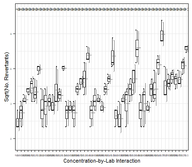
Figure 1: Boxplot for concentration-by-laboratory interaction in compound 4

3 Williams-by-total mean interaction contrasts

In the following, the interaction contrasts are derived for the two-way layout dose-by-laboratory. First, the Williams-contrast test is derived for the primary factor ’dose’, then the contrast test for comparison with the total mean for the secondary factor ’laboratories’, and finally the resulting interaction contrast.

3.1 Factor dose: The Williams-type multiple contrast test

Williams original procedure [26] is a rather complex approach based on maximum likelihood estimators under total order restriction, hard to generalize. Here we use its re-formulation as multiple contrast test [2], assuming order restriction with respect to C-. A multiple contrast test is a maximum test on $q$ elementary tests (where $q$ depends on the kind of multiple contrast) (i.e. a special version of an union-intersection test): $t_{MCT}=max(t_{1},...,t_{q})$ which follows jointly $(t_{1},\ldots,t_{q})^{\prime}$ a $q$-variate $t$- distribution with a common degree of freedom $df$ and the correlation matrix $R$, which is depending on $c_{i},n_{i}$ under simple assumptions (or more complex for other MCT’s [9]). The included single contrast tests $t_{SC}=\sum_{i=0}^{k}c_{i}\bar{x}_{i}/S\sqrt{\sum_{i}^{k}c_{i}^{2}/n_{i}}$ and $\sum_{i=0}^{k}c_{i}=0$ differ by their weights $c_{i}$, i.e. particular contrast matrix definitions determine the particular test version. For the simple balanced design with k=3 the contrast matrix for the one-sided Williams-type test is:

$c_{i}$	C	$D_{1}$	$D_{2}$	$D_{3}$
$c_{a}$	-1	0	0	1
$c_{b}$	-1	0	1/2	1/2
$c_{c}$	-1	1/3	1/3	1/3

The simple Williams contrast illustrates the idea and interoperability of an MCT: either the comparison of $D_{3}$ vs. C is significant (i.e. strict monotone), or to the pooled $(D_{3}+D_{2})/2$, or $(D_{3}+D_{2}+D_{1})/3$, i.e. a plateau (or all three, or neither ($H_{0}$). Either multiplicity-adjusted p-values or simultaneous confidence limits (here one-sided lower limits) are available: $[\sum_{i=0}^{k}c_{i}\bar{x}_{i}-S*t_{q,df,R,2-sided,1-\alpha}\sqrt{\sum_{i}^{k}c_{i}^{2}/n_{i}}]$.

This makes the Williams test the recommended trend test in pharmacology/toxicology: sensitive to some monotonic and partially non-monotonic forms, a comparison to the control, easily interpretable confidence intervals for the required effect sizes. In regulatory toxicology not only the difference of means is relevant as effect size [23], such as proportions or counts. Therefore, the Williams test is available for difference [10], risk ratio or odds ratio of proportions [9], ratio-to-control estimates [11], the nonparametric relative effect sizes [14], hazard rates [7], multiple endpoints [6], heteroscedastic error terms [8] and poly-k-adjusted tumor rates [20]).

3.2 Factor laboratory: The total mean multiple contrast test

Qualitative levels of a factor (without order restriction) are commonly compared by Tukey’s all-pairs comparison procedure [25]. Their numerous, exact $(l*(l-1)/2)*2$ comparisons make this procedure conservative and especially difficult to interpret. One or more deviating laboratories can also be identified by total mean comparisons [18], but with only $l$ to be interpreted. For $l=4$ laboratories the contrast matrix is (in a balanced design) simply

$c_{i}$	$Lab_{A}$	$Lab_{B}$	$Lab_{C}$	$Lab_{D}$
$c_{a}$	-1	1/3	1/3	1/3
$c_{b}$	1/3	-1	1/3	1/3
$c_{c}$	1/3	1/3	-1	1/3
$c_{d}$	1/3	1/3	1/3	-1

3.3 Interaction dose-by-laboratory: Williams-by-total mean interaction contrast test

When reformulating the common ANOVA interaction model: $y_{klj}=\mu+\alpha_{k}+\beta_{l}+(\alpha\beta)_{kl}+\epsilon_{klj}$ (with $j$ replicates) into a cell means model $y_{klj}=\mu_{kl}+\epsilon_{klj}$ the null hypothesis of interaction can be written:
$H_{0}:(\mu_{kl}-\mu_{kl^{\prime}})-(\mu_{k^{\prime}l}-\mu_{k^{\prime}l^{\prime}})=0$ for all $(k,k^{\prime})$ and $(l,l^{\prime})$ [13] as a special form of product-type interactions [5]. Using the both contrast matrices for Williams-type between doses $C_{Dose}$ and between laboratories total mean $C_{l}ab$, the interaction contrast is the Kronecker product $C_{Dose,lab}=C_{Dose}\otimes C_{lab}$. This can easily be realized for different two-way contrast types with the CRAN-package statint [24]. Explicit for the above Ames assay example Table 1 contains the 36 individual contrasts for Williams-by-total mean interaction with k=7 $([0,0.015625,0.03125,0.0625,0.125,0.25,0.5]$ and l=6 $[Lab_{1},Lab_{3},Lab_{4},Lab_{5},Lab_{6},Lab_{7}])$:

No.	IA-contrast lab:dose abbreviation	Contrast type
1	((1 - 2,3,4,5,6,7):0.5) - ((1 - 2,3,4,5,6,7):0)	(Lab1 vs. all Labs) by Williams contrast 1 $(0.5-C-)$
2	((1 - 2,3,4,5,6,7):0.25,0.5) - ((1 - 2,3,4,5,6,7):0)	(Lab1 vs. all Labs) by Williams contrast 2 $((0.5+0.25)/2-C-)$
3	((1 - 2,3,4,5,6,7):0.125,0.25,0.5) - ((1 - 2,3,4,5,6,7):0)	(Lab1 vs. all Labs) by Williams contrast 3 $((0.5+0.25+0.125)/3-C-)$
4	((1 - 2,3,4,5,6,7):0.0625,0.125,0.25,0.5) - ((1 - 2,3,4,5,6,7):0)	(Lab1 vs. all Labs) by Williams contrast 4 $((0.5+0.25+0.125+0.0625)/4-C-)$
5	((1 - 2,3,4,5,6,7):0.03125,0.0625,0.125,0.25,0.5) - ((1 - 2,3,4,5,6,7):0)	(Lab1 vs. all Labs) by Williams contrasts 5 $((0.5+0.25+0.125+0.0625+0.031)/5-C-)$
6	((1 - 2,3,4,5,6,7):0.015625,0.03125,0.0625,0.125,0.25,0.5) - ((1 - 2,3,4,5,6,7):0)	(Lab1 vs. all Labs) by Williams contrast 6 $((0.5+0.25+0.125+0.0625+0.031+0.015)/6-C-)$
7	((2 - 1,3,4,5,6,7):0.5) - ((2 - 1,3,4,5,6,7):0)	(Lab2 vs. all Labs) by Williams contrast 1
8	((2 - 1,3,4,5,6,7):0.25,0.5) - ((2 - 1,3,4,5,6,7):0)	(Lab2 vs. all Labs) by Williams contrast 2
9	((2 - 1,3,4,5,6,7):0.125,0.25,0.5) - ((2 - 1,3,4,5,6,7):0)	(Lab2 vs. all Labs) by Williams contrast 3
10	((2 - 1,3,4,5,6,7):0.0625,0.125,0.25,0.5) - ((2 - 1,3,4,5,6,7):0)	(Lab2 vs. all Labs) by Williams contrast 4
11	((2 - 1,3,4,5,6,7):0.03125,0.0625,0.125,0.25,0.5) - ((2 - 1,3,4,5,6,7):0)	(Lab2 vs. all Labs) by Williams contrast 5
12	((2 - 1,3,4,5,6,7):0.015625,0.03125,0.0625,0.125,0.25,0.5) - ((2 - 1,3,4,5,6,7):0)	(Lab2 vs. all Labs) by Williams contrast 6
13	((3 - 1,2,4,5,6,7):0.5) - ((3 - 1,2,4,5,6,7):0)	(Lab3 vs. all Labs) by Williams contrast 1
14	((3 - 1,2,4,5,6,7):0.25,0.5) - ((3 - 1,2,4,5,6,7):0)	(Lab3 vs. all Labs) by Williams contrast 2
15	((3 - 1,2,4,5,6,7):0.125,0.25,0.5) - ((3 - 1,2,4,5,6,7):0)	(Lab3 vs. all Labs) by Williams contrast 3
16	((3 - 1,2,4,5,6,7):0.0625,0.125,0.25,0.5) - ((3 - 1,2,4,5,6,7):0)	(Lab3 vs. all Labs) by Williams contrast 4
17	((3 - 1,2,4,5,6,7):0.03125,0.0625,0.125,0.25,0.5) - ((3 - 1,2,4,5,6,7):0)	(Lab3 vs. all Labs) by Williams contrast 5
18	((3 - 1,2,4,5,6,7):0.015625,0.03125,0.0625,0.125,0.25,0.5) - ((3 - 1,2,4,5,6,7):0)	(Lab3 vs. all Labs) by Williams contrast 6
19	((4 - 1,2,3,5,6,7):0.5) - ((4 - 1,2,3,5,6,7):0)	(Lab4 vs. all Labs) by Williams contrast 1
20	((4 - 1,2,3,5,6,7):0.25,0.5) - ((4 - 1,2,3,5,6,7):0)	(Lab4 vs. all Labs) by Williams contrast 2
21	((4 - 1,2,3,5,6,7):0.125,0.25,0.5) - ((4 - 1,2,3,5,6,7):0)	(Lab4 vs. all Labs) by Williams contrast 3
22	((4 - 1,2,3,5,6,7):0.0625,0.125,0.25,0.5) - ((4 - 1,2,3,5,6,7):0)	(Lab4 vs. all Labs) by Williams contrast 4
23	((4 - 1,2,3,5,6,7):0.03125,0.0625,0.125,0.25,0.5) - ((4 - 1,2,3,5,6,7):0)	(Lab4 vs. all Labs) by Williams contrast 5
24	((4 - 1,2,3,5,6,7):0.015625,0.03125,0.0625,0.125,0.25,0.5) - ((4 - 1,2,3,5,6,7):0)	(Lab4 vs. all Labs) by Williams contrast 6
25	((5 - 1,2,3,4,6,7):0.5) - ((5 - 1,2,3,4,6,7):0)	(Lab5 vs. all Labs) by Williams contrast 1
26	((5 - 1,2,3,4,6,7):0.25,0.5) - ((5 - 1,2,3,4,6,7):0)	(Lab5 vs. all Labs) by Williams contrast 2
27	((5 - 1,2,3,4,6,7):0.125,0.25,0.5) - ((5 - 1,2,3,4,6,7):0)	(Lab5 vs. all Labs) by Williams contrast 3
28	((5 - 1,2,3,4,6,7):0.0625,0.125,0.25,0.5) - ((5 - 1,2,3,4,6,7):0)	(Lab5 vs. all Labs) by Williams contrast 4
29	((5 - 1,2,3,4,6,7):0.03125,0.0625,0.125,0.25,0.5) - ((5 - 1,2,3,4,6,7):0)	(Lab5 vs. all Labs) by Williams contrast 5
30	((5 - 1,2,3,4,6,7):0.015625,0.03125,0.0625,0.125,0.25,0.5) - ((5 - 1,2,3,4,6,7):0)	(Lab5 vs. all Labs) by Williams contrast 6
31	((6 - 1,2,3,4,5,7):0.5) - ((6 - 1,2,3,4,5,7):0)	(Lab6 vs. all Labs) by Williams contrast 1
32	((6 - 1,2,3,4,5,7):0.25,0.5) - ((6 - 1,2,3,4,5,7):0)	(Lab6 vs. all Labs) by Williams contrast 2
33	((6 - 1,2,3,4,5,7):0.125,0.25,0.5) - ((6 - 1,2,3,4,5,7):0)	(Lab6 vs. all Labs) by Williams contrast 3
34	((6 - 1,2,3,4,5,7):0.0625,0.125,0.25,0.5) - ((6 - 1,2,3,4,5,7):0)	(Lab6 vs. all Labs) by Williams contrast 4
35	((6 - 1,2,3,4,5,7):0.03125,0.0625,0.125,0.25,0.5) - ((6 - 1,2,3,4,5,7):0)	(Lab6 vs. all Labs) by Williams contrast 5
36	((6 - 1,2,3,4,5,7):0.015625,0.03125,0.0625,0.125,0.25,0.5) - ((6 - 1,2,3,4,5,7):0)	(Lab6 vs. all Labs) by Williams contrast 6
37	((7 - 1,2,3,4,5,6):0.5) - ((7 - 1,2,3,4,5,6):0)	(Lab7 vs. all Labs) by Williams contrast 1
38	((7 - 1,2,3,4,5,6):0.25,0.5) - ((7 - 1,2,3,4,5,6):0)	(Lab7 vs. all Labs) by Williams contrast 2
39	((7 - 1,2,3,4,5,6):0.125,0.25,0.5) - ((7 - 1,2,3,4,5,6):0)	(Lab7 vs. all Labs) by Williams contrast 3
40	((7 - 1,2,3,4,5,6):0.0625,0.125,0.25,0.5) - ((7 - 1,2,3,4,5,6):0)	(Lab7 vs. all Labs) by Williams contrast 4
41	((7 - 1,2,3,4,5,6):0.03125,0.0625,0.125,0.25,0.5) - ((7 - 1,2,3,4,5,6):0)	(Lab7 vs. all Labs) by Williams contrast 5
42	((7 - 1,2,3,4,5,6):0.015625,0.03125,0.0625,0.125,0.25,0.5) - ((7 - 1,2,3,4,5,6):0)	(Lab7 vs. all Labs) by Williams contrast 6

Table 1: Interaction contrast structure for Williams trend-by-total means

This table of this already ample example makes clear the advantages and disadvantages of this approach: on the one hand, 36 individual decisions instead of one single F-test, on the other hand, the individual decisions allow the statement between which laboratories and which trend contrasts there is similarity and where not. In terms of an union-intersection test (UIT), the approach is conservative, but not so extreme because of the high correlation between the contrasts. If you want to know which interactions are equivalent and which are not, use a combined intersection-union-by-union-intersection test (IUT-UIT): IUT for the equivalence tests in both directions, and UIT between the IA contrasts. It is also possible to achieve a global statement by using an IUT-IUT (then the IA-test at the marginal $\alpha=0.05$ level), where all individual tests should fulfill $p>0.10$.

3.4 A possible simplification: $(D_{k}-C-)$-by-total mean interaction contrasts

Assuming a monotonic dose-response dependence, the entire William contrast can be replaced by $(D_{k}-C-)$ comparison in a simplified way. This is surprising, but $(D_{k}-C-)$ is the most important single contrast in the William test, is part of the corresponding closure test [9] and part of the strict trend test according [15]. This reduction especially simplifies the interpretation to only $k$ interaction contrasts. This simplification should be avoided if downturns at higher dose(s) are possible or if you are more interested in comparing the NOAEC instead of a trend itself. The simplification becomes clear looking on Table 2 for the above Ames assay example: only 7 contrasts, claiming for local equivalence for laboratories $[1,2,3,4,5,6]$ and but not for global equivalence because laboratory 7 behaves borderline non-equivalent.

Number	Interaction contrast	p-value
1	((1 - 2,3,4,5,6,7):0.5) - ((1 - 2,3,4,5,6,7):0)	0.985
2	((2 - 1,3,4,5,6,7):0.5) - ((2 - 1,3,4,5,6,7):0)	0.410
3	((3 - 1,2,4,5,6,7):0.5) - ((3 - 1,2,4,5,6,7):0)	0.999
4	((4 - 1,2,3,5,6,7):0.5) - ((4 - 1,2,3,5,6,7):0)	0.999
5	((5 - 1,2,3,4,6,7):0.5) - ((5 - 1,2,3,4,6,7):0)	0.584
6	((6 - 1,2,3,4,5,7):0.5) - ((6 - 1,2,3,4,5,7):0)	0.120
7	((7 - 1,2,3,4,5,6):0.5) - ((7 - 1,2,3,4,5,6):0)	0.100

Table 2: Compound 4: interaction contrast for C vs. $D_{k}$ by grand means between labs- S9+

3.5 A modification

Variance heterogeneity often occurs in these assays and their ignorance can lead to significant bias. Therefore you should use the sandwich variance estimator (see below using vcov=sandwich argument in the function glht()) [8].

4 Evaluation of the example using the CRAN packages statint and multcomp

The following R-code can be used for the Ames assay example for the data object A984p:

library(multcomp); library(statint); library(sandwich)
InteractionContrastsP984t <- iacontrast(fa=A984p$lab,fb=A984p$Conc,
                                       typea="totalMean", typeb="Williams")
A984p$labConct <- InteractionContrastsP984t$fab
CellMeansModelP984t <- lm(Trans ~ labConct-1, data=A984p) # cell means model
MultTestP984t <- glht(model=CellMeansModelP984t,
                 linfct = mcp(labConct=InteractionContrastsP984t$cmab), vcov=sandwich)
piap984t<-summary(MultTestP984t)ΨΨΨΨΨΨ#calculating adjusted p-values

Number	Interaction contrast	p-value
1	((1 - 2,3,4,5,6,7):0.5) - ((1 - 2,3,4,5,6,7):0)	0.9994
2	((1 - 2,3,4,5,6,7):0.25,0.5) - ((1 - 2,3,4,5,6,7):0)	0.999
3	((1 - 2,3,4,5,6,7):0.125,0.25,0.5) - ((1 - 2,3,4,5,6,7):0)	0.999
4	((1 - 2,3,4,5,6,7):0.0625,0.125,0.25,0.5) - ((1 - 2,3,4,5,6,7):0)	0.9698
5	((1 - 2,3,4,5,6,7):0.03125,0.0625,0.125,0.25,0.5) - ((1 - 2,3,4,5,6,7):0)	0.8706
6	((1 - 2,3,4,5,6,7):0.015625,0.03125,0.0625,0.125,0.25,0.5) - ((1 - 2,3,4,5,6,7):0)	0.9230
7	((2 - 1,3,4,5,6,7):0.5) - ((2 - 1,3,4,5,6,7):0)	0.5901
8	((2 - 1,3,4,5,6,7):0.25,0.5) - ((2 - 1,3,4,5,6,7):0)	0.4831
9	((2 - 1,3,4,5,6,7):0.125,0.25,0.5) - ((2 - 1,3,4,5,6,7):0)	0.8529
10	((2 - 1,3,4,5,6,7):0.0625,0.125,0.25,0.5) - ((2 - 1,3,4,5,6,7):0)	0.8546
11	((2 - 1,3,4,5,6,7):0.03125,0.0625,0.125,0.25,0.5) - ((2 - 1,3,4,5,6,7):0)	0.9306
12	((2 - 1,3,4,5,6,7):0.015625,0.03125,0.0625,0.125,0.25,0.5) - ((2 - 1,3,4,5,6,7):0)	0.9719
13	((3 - 1,2,4,5,6,7):0.5) - ((3 - 1,2,4,5,6,7):0)	0.999
14	((3 - 1,2,4,5,6,7):0.25,0.5) - ((3 - 1,2,4,5,6,7):0)	0.999
15	((3 - 1,2,4,5,6,7):0.125,0.25,0.5) - ((3 - 1,2,4,5,6,7):0)	0.9990
16	((3 - 1,2,4,5,6,7):0.0625,0.125,0.25,0.5) - ((3 - 1,2,4,5,6,7):0)	0.9887
17	((3 - 1,2,4,5,6,7):0.03125,0.0625,0.125,0.25,0.5) - ((3 - 1,2,4,5,6,7):0)	0.999
18	((3 - 1,2,4,5,6,7):0.015625,0.03125,0.0625,0.125,0.25,0.5) - ((3 - 1,2,4,5,6,7):0)	0.999
19	((4 - 1,2,3,5,6,7):0.5) - ((4 - 1,2,3,5,6,7):0)	0.999
20	((4 - 1,2,3,5,6,7):0.25,0.5) - ((4 - 1,2,3,5,6,7):0)	0.999
21	((4 - 1,2,3,5,6,7):0.125,0.25,0.5) - ((4 - 1,2,3,5,6,7):0)	0.999
22	((4 - 1,2,3,5,6,7):0.0625,0.125,0.25,0.5) - ((4 - 1,2,3,5,6,7):0)	0.999
23	((4 - 1,2,3,5,6,7):0.03125,0.0625,0.125,0.25,0.5) - ((4 - 1,2,3,5,6,7):0)	0.999
24	((4 - 1,2,3,5,6,7):0.015625,0.03125,0.0625,0.125,0.25,0.5) - ((4 - 1,2,3,5,6,7):0)	0.999
25	((5 - 1,2,3,4,6,7):0.5) - ((5 - 1,2,3,4,6,7):0)	0.7772
26	((5 - 1,2,3,4,6,7):0.25,0.5) - ((5 - 1,2,3,4,6,7):0)	0.8020
27	((5 - 1,2,3,4,6,7):0.125,0.25,0.5) - ((5 - 1,2,3,4,6,7):0)	0.9052
28	((5 - 1,2,3,4,6,7):0.0625,0.125,0.25,0.5) - ((5 - 1,2,3,4,6,7):0)	0.9928
29	((5 - 1,2,3,4,6,7):0.03125,0.0625,0.125,0.25,0.5) - ((5 - 1,2,3,4,6,7):0)	0.9828
30	((5 - 1,2,3,4,6,7):0.015625,0.03125,0.0625,0.125,0.25,0.5) - ((5 - 1,2,3,4,6,7):0)	0.9999
31	((6 - 1,2,3,4,5,7):0.5) - ((6 - 1,2,3,4,5,7):0)	0.1843
32	((6 - 1,2,3,4,5,7):0.25,0.5) - ((6 - 1,2,3,4,5,7):0)	0.2064
33	((6 - 1,2,3,4,5,7):0.125,0.25,0.5) - ((6 - 1,2,3,4,5,7):0)	0.7596
34	((6 - 1,2,3,4,5,7):0.0625,0.125,0.25,0.5) - ((6 - 1,2,3,4,5,7):0)	0.8450
35	((6 - 1,2,3,4,5,7):0.03125,0.0625,0.125,0.25,0.5) - ((6 - 1,2,3,4,5,7):0)	0.9857
36	((6 - 1,2,3,4,5,7):0.015625,0.03125,0.0625,0.125,0.25,0.5) - ((6 - 1,2,3,4,5,7):0)	0.9952
37	((7 - 1,2,3,4,5,6):0.5) - ((7 - 1,2,3,4,5,6):0)	0.1511
38	((7 - 1,2,3,4,5,6):0.25,0.5) - ((7 - 1,2,3,4,5,6):0)	0.4369
39	((7 - 1,2,3,4,5,6):0.125,0.25,0.5) - ((7 - 1,2,3,4,5,6):0)	0.3633
40	((7 - 1,2,3,4,5,6):0.0625,0.125,0.25,0.5) - ((7 - 1,2,3,4,5,6):0)	0.4856
41	((7 - 1,2,3,4,5,6):0.03125,0.0625,0.125,0.25,0.5) - ((7 - 1,2,3,4,5,6):0)	0.7422
42	((7 - 1,2,3,4,5,6):0.015625,0.03125,0.0625,0.125,0.25,0.5) - ((7 - 1,2,3,4,5,6):0)	0.8666

Table 3: Compound 4: interaction contrast for Williams trend-by grand means between labs- S9+

The related adjusted p-values for this IUT-UIT test in Table 3 are predominantly large, which indicate equivalence, even global equivalence. Only one contrast, No. 37 shows with $p=0.1511$ a tendency of non-equivalence; but the single comparison $(D_{k}-C-)$ should not be relevant for the Ames assay because the decision is based on the lower doses. This p-value of $0.1511$ is part of the comparisons of Lab 7 against all others, which are not as large as the others (but still equivalent). Notice, Lab 7 used a different source of bacteria revealing a higher spontaneous reversion rate.

Even more informative is the plot of the simultaneous two-sided $(1-2\alpha)$ confidence intervals in Figure 2, demonstrating the problems with Lab 7 in the scale of transformed revertant count differences. Notice, using the IUT-IUT approach with marginal levels, global equivalence can be claimed for this selected example.

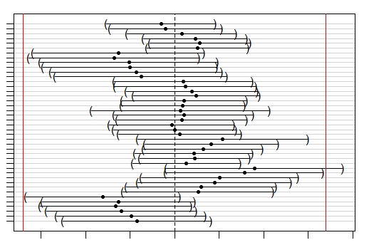
Figure 2: 42 interaction contrasts: compatible simultaneous confidence intervals

Notice, the (two-sided) p-value for the common F-test on dose-by-laboratory interaction is $0.10$ indicating that an interaction cannot be excluded. However, it is not clear for which laboratories and which dose comparisons - a nice proof of the usefulness of the above IA-contrast method in this example.

5 Summary

Similarity of multiple dose-response curves in interlaboratory studies in regulatory toxicology can be demonstrated using dose-by-laboratory interaction contrasts [12, 9]. To illustrate a trend of the dose-response curve, Williams-by-Laboratory interaction contrasts are proposed here. With help of the CRAN packages statint and multcomp the estimation of adjusted p-values or compatible simultaneous confidence intervals is relatively easy. The interpretation in terms of global or partial equivalence (similarity) is challenging, but impressive.

References

- [1] P. Bauer and M. Kieser. A unifying approach for confidence intervals and testing of equivalence and difference. Biometrika 83: 934 – 937, 1996.
- [2] F. Bretz. An extension of the Williams trend test to general unbalanced linear models. Comput. Statist. and Data Analysis, 50(7):1735–1748, April 2006.
- [3] S.D. Dertinger, et al. Intra- and inter-laboratory reproducibility of the rat blood Pig-a gene mutation assay. Environ. Mol. Mutagen. 61:500–507, 2020.
- [4] I. Flueckiger-Isler and M. Kamber. Direct comparison of the Ames microplate format (MPF) test in liquid medium with the standard Ames pre-incubation assay on agar plates by use of equivocal to weakly positive test compounds. Mutat. Res./Genet. Toxic. and Environ. Mutagen. 747: 36–45, 2012.
- [5] K.R. Gabriel and J. Putter and Y. Wax. Simultaneous confidence intervals for product-type interaction contrasts. J.R.S.S.-B 35: 234 – 244, 1973.
- [6] M. Hasler and L.A. Hothorn. A multivariate Williams-type trend procedure. Statist. in Biopharm. Res., 4(1):57–65, 2012.
- [7] E. Herberich and L.A. Hothorn. Statistical evaluation of mortality in long-term carcinogenicity bioassays using a Williams-type procedure. Regul. Toxicol. Pharm., 64:26–34, 2012.
- [8] E. Herberich, J. Sikorski, and T. Hothorn. A robust procedure for comparing multiple means under heteroscedasticity in unbalanced designs. PLOS One, 5(3):e9788, March 2010.
- [9] L.A. Hothorn. Statistics in Toxicology- using R. Chapman Hall, 2016.
- [10] L.A. Hothorn and M. Sill and F. Schaarschmidt. Evaluation of incidence rates in pre-clinical studies using a Williams-type procedure. The Int. J. of Biostat. 6: 1,15, 2010.
- [11] L.A. Hothorn and G.D. Djira. A ratio-to-control Williams-type test for trend. Pharm. Statist., 10(4):289–292, July 2011.
- [12] L.A. Hothorn Statistics of interlaboratory in vitro toxicological studies. ATLA.31: 43–63.2003.
- [13] A. Kitsche and F. Schaarschmidt. Analysis of statistical interactions in factorial experiments. J. Agr. Crop Sci. 201: 69 –79, 2014.
- [14] F. Konietschke and L.A. Hothorn. Evaluation of toxicological studies using a nonparametric Shirley-type trend test for comparing several dose levels with a control group. Statist.in Biopharm. Res., 4(1):14–27, 2012.
- [15] K.K. Lin and M.A. Rahman. Comparisons of false negative rates from a trend test alone and from a trend test jointly with a control-high groups pairwise test in the determination of the carcinogenicity of new drugs. J. Biopharm. Stat., 29(1):128–142, 2019.
- [16] H. Nishiyama and T. Omori and I. Yoshimura. A composite statistical procedure for evaluating genotoxicity using cell transformation assay data. Environmetrics 14: 183 –192, 2003.
- [17] OECD Guideline for testing of chemicals No. 474. In vivo micronucleus test, 2006.
- [18] P. Pallmann and L.A. Hothorn. Analysis of means (ANOM): a generalized approach using R. J. Appl. Stat. doi:10.1080/02664763.2015.1117584, 2016.
- [19] G. Reifferscheid and H.M. Maes et al. International Round-Robin Study on the Ames Fluctuation Test. Environm. and Mol. Mutagen. 53:185–197,2012.
- [20] F. Schaarschmidt and M. Sill and L.A. Hothorn. Poly-k-tend tests for survival adjusted analysis of tumor rates formulated as approximate multiple contrast test. J. Biopharm. Stat. 18: 934 –948, 2008.
- [21] D. Spiliotopoulos and C. Koelbert Assessment of the miniaturized liquid Ames microplate format (MPF) for a selection of the test items from the recommended list of genotoxic and non-genotoxic chemicals. Mutat. Res. 856–857:503218,2020.
- [22] D. Spiliotopoulos et al. An interlaboratory study to validate Ames MPF assay. Mut. Res., to appear.
- [23] E. Szoecs and R.B. Schaefer. A comparison of statistical approaches for analysis of count and proportion data in ecotoxicology. Environ. Sci. Pollut. Res. 22:13990–13999,2015.
- [24] A. Kitsche and F. Schaarschmidt. Generating labeled product type interaction contrasts. CRAN package
- [25] J. Tukey. The problem of multiple comparisons. Princeton University, 1953.
- [26] D.A. Williams. A test for differences between treatment means when several dose levels are compared with a zero dose control. Biometrics, 27(1):103–117, 1971.