From Gaudin Integrable Models to $d$-dimensional Multipoint Conformal Blocks

Abstract

In this work we initiate an integrability-based approach to multipoint conformal blocks for higher dimensional conformal field theories. Our main observation is that conformal blocks for $N$-point functions may be considered as eigenfunctions of integrable Gaudin Hamiltonians. This provides us with a complete set of differential equations that can be used to evaluate multipoint blocks.

DESY 20-157
ZMP-HH/20-25
SAGEX-20-22-E

I Introduction

Conformal quantum field theories (CFTs) play an important role for our understanding of phase transitions, quantum field theory and even the quantum physics of gravity, through Maldacena’s celebrated holographic duality. Since they are often strongly coupled, however, they are very difficult to access with traditional perturbative methods. Polyakov’s famous conformal bootstrap program provides a powerful non-perturbative handle that allows to calculate critical exponents and other dynamical observables using only general features such as (conformal) symmetry, locality and unitarity Polyakov:1974gs . The program has had impressive success in $d=2$ dimensions Belavin:1984vu where it produced numerous exact solutions. During the last decade, the bootstrap has seen a remarkable revival in higher dimensional theories with new numerical as well as analytical incarnations. This has produced many stunning new insights, see e.g. Poland_2019 for a review and references, including record precision computations of critical exponents in the critical 3D Ising model Kos:2016ysd ; Simmons-Duffin:2016wlq . Despite these advances, it is evident that significant further developments are needed to make these techniques more widely applicable, beyond a few special theories.

One promising avenue would be to study bootstrap consistency conditions for $N$-point correlators with $N>4$ fields. Note that the success in $d=2$ is ultimately based on the ability to analyze correlation functions with any number of stress tensor insertions. But the extension of the bootstrap constraints in $d>2$ beyond 4-point functions has been hampered by very significant technical problems, see Rosenhaus:2018zqn ; Parikh:2019ygo ; Fortin:2019dnq ; Goncalves:2019znr ; Parikh:2019dvm ; Fortin:2019zkm ; Irges:2020lgp ; Fortin:2020yjz ; Fortin:2020ncr ; Zhou:2020ptb ; Pal:2020dqf ; Fortin:2020bfq ; Hoback:2020pgj for recent publications. To overcome these challenges is the main goal of our work.

The central tool for CFTs in general and for the conformal bootstrap in particular are conformal partial wave expansions. These were introduced in Ferrara:1973vz to separate correlation functions into kinematically determined conformal blocks (partial waves) and expansion coefficients which contain all the dynamical information. For 4-point correlators, the relevant blocks are now well understood in any $d$, though only after some significant effort. Here we shall lay the foundations for a systematic extension to multipoint (MP) blocks. Our approach extends a remarkable observation in Isachenkov:2016gim about a relation between 4-point blocks and exactly solvable (integrable) Schroedinger problems.

To understand the key challenge in developing a theory of MP conformal blocks, let us consider a 5-point function of scalar fields. In more than two dimensions one can build five independent conformally invariant cross ratios from $N=5$ points. Correlation functions can be evaluated through repeated use of Wilson’s operator product expansion (OPE). We may picture this process with the help of an OPE diagram, such as the one shown in Fig. 1. For $N=5$ points, any such diagram contains two intermediate fields. The scaling weights $\Delta$ and spins $l$ of these intermediate fields provide four quantum numbers. This is not sufficient to resolve the dependence of the $5$-point function on the five cross ratios. The missing fifth quantum number is somehow associated with the choice of so-called tensor structures at the vertices of an OPE diagram. In the case of the 5-point function in $d>2$, the middle vertex in Fig. 1 gives rise to one additional quantum number. But what precisely is the nature of this quantum number and how can it be measured?

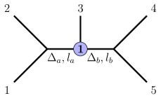
Figure 1: OPE diagram for a 5-point function. The corresponding 5-point conformal block depends on five quantum numbers which are measured by four Casimir operators and one new vertex DO.

In order to describe our answer let us turn to the most basic description of conformal blocks, the so-called shadow formalism Ferrara:1972uq . The latter provides integral formulas for conformal blocks that are reminiscent of Feynman integrals. Finding analytical expressions in terms of special functions or even just efficient numerical evaluations requires significant technology. One crucial tool in the theory of Feynman integrals is to consider them as solutions of some differential equations. In their important work, Dolan and Osborn followed this same strategy and characterized shadow integrals as eigenfunctions of a set of Casimir differential operators (DOs) Dolan:2003hv . By studying these differential equations they were able to harvest decisive new results on the conformal blocks Dolan:2003hv ; Dolan:2011dv .

Shadow integral representations for MP blocks are also known. In order to evaluate these, one may want to follow very much the same strategy that was used for 4-point functions. It is indeed relatively straightforward to write down MP generalizations of the Casimir operators of Dolan:2003hv . In the case of 5-point functions in $d>2$ there are four of them. Their eigenvalues measure the weight and spin of the intermediate fields. But as we explained above, this is not sufficient. We need one more DO that commutes with the four Casimir operators to measure a fifth quantum number. This appears to set the stage for some integrable system and indeed, as we shall show below, the four Casimir operators along with the fifth missing one can be constructed as commuting Hamiltonians of the famous Gaudin integrable model gaudin1976diagonalisation ; Gaudin_book83 , in a certain limit. The statement may be established more generally but the 5-point function of scalar fields is the first case for which we have worked out these DOs explicitly.

Let us now outline the content of this short note. In the next section we review how to construct shadow integral representations for MP functions with a particular focus on the choice of tensor structures at the vertices. We introduce a novel basis of 3-point tensor structures that enables us to characterize the shadow integral, and hence the blocks, as common eigenfunctions of a set of five commuting DOs. In section 3, we explain how these operators can be constructed systematically from Hamiltonians of the Gaudin integrable model by taking a special limit. Four of the five DOs are Casimir operators while the fifth one measures the choice of tensor structure. We conclude with an outlook on our forthcoming paper Buric:2020 , extensions and applications to the higher dimensional conformal bootstrap.

II Multipoint Shadow Integrals

In order to state our results precisely, we shall briefly review some basics of the shadow integral formalism. The shadow formalism turns the graphical representation of a conformal block, such as that of Fig. 1, into an integral formula. Just as in the case of Feynman integrals, the ‘shadow integrand’ is built from relatively simple building blocks that are assigned to the links and 3-point vertices in the associated OPE diagram. For a scalar 5-point function, the most complicated vertex contains one scalar leg and two that are carrying symmetric traceless tensor (STT) representations. In order to write this vertex, we shall employ polarization spinors $z\in\mathbb{C}^{d}$ (see Dobrev:1976aa ; Dobrev:1977qv ; Costa:2011aa ; Costa:2011ab ) to convert spinning operators in STT representations into objects of the form

$$\mathcal{O}_{\Delta,l}(x;z)=\mathcal{O}_{\Delta,l}^{\nu_{1}...\nu_{l}}(x)z_{\nu_{1}}...z_{\nu_{l}}\equiv\mathcal{O}^{\underline{\nu}}_{\Delta,l}(x)z_{\underline{\nu}}\ .$$ (1)

The usual contraction of the STTs can be re-expressed as an integral over $\mathbb{C}^{d}$ as follows Bargmann_1977

$$\mathcal{O}^{\underline{\nu}}(x)\mathcal{O}^{\prime}_{\underline{\nu}}(x^{\prime})=\!\int_{\mathbb{C}^{d}}\!\!\differential^{2d}z\,\delta(z^{2})\rho(\bar{z}\cdot z)\,\mathcal{O}(x;\bar{z})\mathcal{O}^{\prime}(x^{\prime};z),$$ (2)

$$\rho(t)=\left(\frac{2}{\pi}\right)^{d-1}\frac{(16t)^{1-d/4}}{\Gamma(d/2-1)}K_{(d/2-2)}(2\sqrt{t}),$$ (3)

where $\mathcal{O}$ and $\mathcal{O}^{\prime}$ are fields of equal spin and $K$ is the modified Bessel function of the second kind. In building shadow integrands, the function $\rho$ plays a role analogous to the propagator in Feynman integrals. Having now converted field multiplets into functions, the 3-point vertex with one scalar leg and two STT legs takes the form

$$\Phi^{t}_{acb}(x;z) =\langle\mathcal{O}_{\Delta_{a},l_{a}}(x_{a};z_{a})\mathcal{O}_{\Delta_{c}}(x_{c})\mathcal{O}_{\Delta_{b},l_{b}}(x_{b};z_{b})\rangle=$$

$$\frac{(X_{bc;a}\cdot z_{a})^{l_{a}}(X_{ca;b}\cdot z_{b})^{l_{b}}}{(X_{ab;c}^{2})^{\frac{-\Delta_{c}}{2}}(X_{ca;b}^{2})^{\frac{l_{b}-\Delta_{b}}{2}}(X_{bc;a}^{2})^{\frac{l_{a}-\Delta_{a}}{2}}}t\left(X\right),$$ (4)

if $l_{a}-l_{b}\in 2\mathbb{Z}$ and vanishes otherwise. Here we have used the standard notation

$$X_{ij;k}^{\mu}:=\frac{x_{ik}^{\mu}}{x_{ik}^{2}}-\frac{x_{jk}^{\mu}}{x_{jk}^{2}}=-X_{ji;k}^{\mu},\,\,\,X_{ij;k}^{2}=\frac{x_{ij}^{2}}{x_{ik}^{2}x_{jk}^{2}},$$ (5)

with $x_{ij}=x_{i}-x_{j}$, and we have dubbed $X$ the unique independent cross-ratio that can be constructed from $(x_{a},x_{b},x_{c};z_{a},z_{b})$,

$$X=\frac{1}{2x_{ab}^{4}}\frac{z_{a\mu}\left(x_{ab}^{2}\delta^{\mu\nu}-2x_{ab}^{\mu}x_{ab}^{\nu}\right)z_{b\nu}}{(z_{a}\cdot X_{bc;a})(z_{b}\cdot X_{ca;b})}\ .$$ (6)

To a large extent, the function $t(X)$ that appears in the 3-point vertex is left undetermined by conformal symmetry. The only constraints come from the action of the $SO(d-1)$ subgroup that stabilizes three points in $\mathbb{R}^{d}$, as well as the parity operator in $\mathrm{O}(d)$. For parity-even vertices, the function $t(X)$ belongs to the space $W^{+}_{t}$ of polynomials of order at most $\textit{min}(l_{a},l_{b})$. Parity-odd vertices with a single scalar leg only exist in $d=3$. In this case, the function $t(X)\in W_{t}^{-}$ must be chosen such that $t(X)/\sqrt{X(1-X)}$ is a polynomial of order at most $\textit{min}(l_{a},l_{b})-1$. In total, the admissible functions $t(X)$ span a vector space of dimension

$$n_{ab}=\sum_{\pm}\textit{dim}\,W_{t}^{\pm}=\left\{\begin{array}[]{ll}2\textit{min}(l_{a},l_{b})+1,&\quad d=3,\\ \textit{min}(l_{a},l_{b})+1,&\quad d>3.\end{array}\right.$$ (7)

The integer $n_{ab}$ counts the number of 3-point tensor structures Costa:2011ab . Note that $n_{ab}=1$ if either $l_{a}=0$ or $l_{b}=0$ which means that $t$ is a constant factor if there are two or three scalar legs. We shall therefore simply drop the corresponding vertex factors $t$ when using formula (4) for vertices with two scalar legs.

Having described the vertex, we can now write down (shadow) integrals for any desired $N$-point function in the so-called comb channel, in which every OPE includes at least one of the external scalar fields. For $N=5$ external scalar fields of weight $\Delta_{i},i=1,\dots,5$ the shadow integrals read

$$\Psi^{(\Delta_{1},...,\Delta_{5})}_{(\Delta_{a},\Delta_{b};l_{a},l_{b};t)}(x_{1},...,x_{5})=$$ (8)

$$=\prod_{s=a,b}\int_{\mathbb{R}^{d}}\differential^{d}x_{s}\int_{\mathbb{C}^{d}}\differential^{2d}z_{s}\delta(z_{s}^{2})\rho(\bar{z}_{s}\cdot z_{s})\Phi_{12\tilde{a}}(x_{1},x_{2},x_{a};\bar{z}_{a})$$

$$\hskip 42.67912pt\times\Phi^{t}_{a3b}(x_{a},x_{3},x_{b};z_{a},z_{b})\Phi_{\tilde{b}45}(x_{b},x_{4},x_{5};\bar{z}_{b})\ .$$

Here the tilde on the indices of the first and third vertex means that we use eq. (4) for two scalar legs but with $\Delta_{a}$ and $\Delta_{b}$ replaced by $d-\Delta_{a}$ and $d-\Delta_{b}$, respectively.

After splitting off some factor $\Omega$ that accounts for the nontrivial covariance law of the scalar fields under conformal transformations,

$$\Psi^{(\Delta_{i})}_{(\Delta_{a},\Delta_{b};l_{a},l_{b};t)}(x_{i})=\Omega^{(\Delta_{i})}(x_{i})\psi^{(\Delta_{12},\Delta_{3},\Delta_{45})}_{(\Delta_{a},\Delta_{b};l_{a},l_{b};t)}(u_{1},...,u_{5}),$$

$$\Omega^{(\Delta_{i})}(x_{i}):=(X_{23;1}^{2})^{\frac{\Delta_{1}}{2}}\,\prod_{i=2}^{4}(X_{i+1,i-1;i}^{2})^{\frac{\Delta_{i}}{2}}\,(X_{34;5}^{2})^{\frac{\Delta_{5}}{2}},$$

with $\Delta_{ij}=\Delta_{i}-\Delta_{j}$ as usual, the shadow integral (8) gives rise to a finite conformal integral that defines the conformal block $\psi$ as a function of five conformally invariant cross ratios $u_{i}$. These integrals depend on the choice of $(\Delta_{a},l_{a})$, $(\Delta_{b},l_{b})$ and the function $t(X)$. Our goal is to compute this uninviting looking integral.

The strategy we have sketched in the introduction is to write down five differential equations for these blocks. Four of these are given by the eigenvalue equations for the second and fourth order Casimir operators for the intermediate channels,

$$\mathcal{D}^{s}_{p}\psi^{(\Delta_{12},\Delta_{3},\Delta_{45})}_{(\Delta_{a},\Delta_{b};l_{a},l_{b};t)}(u)=C_{p}^{s}\psi^{(\Delta_{12},\Delta_{3},\Delta_{45})}_{(\Delta_{a},\Delta_{b};l_{a},l_{b};t)}\ ,$$ (9)

where $p=2,4$ and $C_{p}^{s}$ denotes the eigenvalue of the $p$-th order Casimir operator in the representation $(\Delta_{s},l_{s})$ for $s=a,b$. The explicit form of the DOs $\mathcal{D}^{s}_{p}$ can be worked out and the resulting expressions resemble those in Dolan:2003hv .

But we are missing one more differential equation which we shall construct in the next section. It will turn out that shadow integrals are eigenfunctions of a fifth DO provided we prepare a very special basis $t_{n}(X),n=1,\dots,n_{ab},$ in the space of 3-point tensor structures. We can characterize these functions $t_{n}(X)$ as eigenfunctions of a particular fourth order DO

$$H^{(d,\Delta_{i},l_{i})}=h_{0}(X)+\sum_{q=1}^{4}h_{q}(X)X^{q-1}(1-X)^{q-1}\partial_{X}^{q}\ ,$$ (10)

where $h_{q}=h_{q}^{(d,\Delta_{i},l_{i})}$ are polynomials of order at most three, see Supplemental Material at [URL] for concrete expressions. The operator $H$, which has several remarkable properties, appears to be new. For our discussion it is most important to note that $H$ leaves the two subspaces $W_{t}^{\pm}$ invariant whenever both $l_{a}$ and $l_{b}$ are integer. Consequently, it specifies a special basis $t_{n}$ of functions $t(X)$ in the space of tensor structures,

$$H^{(d,\Delta_{i},l_{i})}t_{n}(X)=\tau_{n}t_{n}(X)\ ,\quad n=0,\dots,n_{ab}\ .$$ (11)

Explicit formulas for the eigenvalues $\tau_{n}$ and the eigenfunctions $t_{n}(X)$ can be worked out, and it is this basis of 3-point tensor structures that we will use to write down differential equations for the associated shadow integrals.

III Multipoint Blocks and Gaudin Hamiltonians

Our goal now is to characterize the shadow integrals through a complete set of five differential equations. These will take the form of eigenvalue equations for a set of commuting Gaudin Hamiltonians. In order to state precise formulas we need a bit of background on Gaudin models gaudin1976diagonalisation ; Gaudin_book83 . Let us begin with a central object, the so-called Lax matrix,

$$\mathcal{L}(w)=\sum_{i=1}^{N}\frac{\mathcal{T}^{(i)}_{\alpha}T^{\alpha}}{w-w_{i}}=\mathcal{L}_{\alpha}(w)T^{\alpha}\ .$$ (12)

Here, $w_{i}$ are a set of complex numbers, $T_{\alpha}$ denotes a basis of generators of the conformal Lie algebra in $d$ dimensions and $T^{\alpha}$ its dual basis with respect to an invariant bilinear form. The object $\mathcal{T}^{(i)}_{\alpha}$ is the standard first order DO that describes the behavior of a scalar primary field $\mathcal{O}(x_{i})$ of weight $\Delta_{i}$ under the conformal transformation generated by $T_{\alpha}$.

Given some conformally invariant symmetric tensor $\kappa_{p}$ of degree $p$ one can construct a family $\mathcal{H}_{p}(w)$ of commuting operators as Feigin:1994in ; Talalaev:2004qi ; Molev:2013

$$\mathcal{H}_{p}(w)=\kappa^{\alpha_{1}\cdots\alpha_{p}}_{p}\mathcal{L}_{\alpha_{1}}(w)\cdots\mathcal{L}_{\alpha_{p}}(w)+\dots\ ,$$ (13)

where the dots represent correction terms expressible as lower degree combinations of the Lax matrix components $\mathcal{L}_{\alpha}(w)$ and their derivatives with respect to $w$. For $p=2$ such correction terms are absent. The correction terms are necessary to ensure that the families commute,

$$[\,\mathcal{H}_{p}(w)\,,\,\mathcal{H}_{q}(w^{\prime})\,]=0\ ,$$ (14)

for all $p,q$ and all $w,w^{\prime}\in\mathbb{C}$. In the case where $d\geq 3$, the conformal algebra possesses two independent invariant tensors of second and fourth degree . We therefore obtain two families of commuting DOs that act on functions of the coordinates $x_{i}$.

It is a well-known fact that these families commute with the diagonal action of the conformal algebra, i.e.

$$[\,\mathcal{T}_{\alpha}\,,\,\mathcal{H}_{p}(w)\,]=0\quad\textit{ where }\ \mathcal{T}_{\alpha}=\sum_{i=1}^{N}\mathcal{T}_{\alpha}^{(i)}\ .$$ (15)

Hence the commuting families $\mathcal{H}_{p}(w)$ of operators descend to DOs on functions $\psi(u)$ of the conformally invariant cross ratios $u$.

The functions $\mathcal{H}_{p}(w)$ provide several continuous families of commuting operators. Only a finite set of these operators are independent. There are many ways of constructing such sets of independent operators, e.g. by taking residues of $\mathcal{H}_{p}(w)$ at the singular points to give just one example. For the moment, any such set still contains $N$ parameters $w_{i},i=1,\dots,N$. Without loss of generality we can set three of these complex numbers to some specific value, e.g. $w_{1}=0,w_{N-1}=1,w_{N}=\infty$ so that we remain with $N-3$ complex parameters our Gaudin Hamiltonians depend on.

Now we adapt the Gaudin model to the study of MP blocks. In the latter context we insist that the set of commuting operators we work with allows us to measure the weights $\Delta$ and spins $l$ of fields that are exchanged in intermediate channels, as do the MP Casimir operators. So, in order for the Gaudin Hamiltonians to be of any use to us, we must ensure that they include all such Casimir operators. For this to be the case, we are forced to make a very special choice of the remaining parameters $w_{r}$ and to consider specific limits of these parameters . Let us explain this here for $N=5$. Setting $w_{2}=\varpi^{2}$ and $w_{3}=\varpi$ we can define

$$\widetilde{\mathcal{H}}_{p}(w):=\lim_{\varpi\rightarrow 0}\varpi^{p}\mathcal{H}_{p}(\varpi w)\quad,\ p=2,4.$$ (16)

The new functions $\widetilde{\mathcal{H}}_{p}$ take values in the space of $p^{\textit{th}}$ order DOs on cross ratios. They possess singularities at three points only, namely at $w=0,1,\infty$. Let us note that taking the limit $\varpi\rightarrow 0$ does not spoil commutativity of these Hamiltonians.

After performing the special limit on the parameters $w_{r}$ we can now extract the MP Casimir operators rather easily. In fact, it is not difficult to check that

$$\mathcal{D}^{a}_{p}=\lim_{w\rightarrow 0}w^{p}\widetilde{\mathcal{H}}_{p}(w)\quad,\quad\mathcal{D}^{b}_{p}=\lim_{w\rightarrow\infty}w^{p}\widetilde{\mathcal{H}}_{p}(w)$$ (17)

for $p=2,4$. Any additional independent operator we can obtain from $\widetilde{\mathcal{H}}_{p}(w)$ may be used to measure a fifth quantum number. One can show that the two second order Casimir operators $\mathcal{D}^{s}_{2},s=a,b$ exhaust all the independent operators that can be obtained from $\widetilde{\mathcal{H}}_{2}(w)$. The family $\widetilde{\mathcal{H}}_{4}(w)$, on the other hand, indeed supplies one independent operator in addition to the fourth order Casimir operators $\mathcal{D}^{s}_{4},s=a,b$. We propose to use the operator $\mathcal{V}_{4}$ defined through

$$\widetilde{\mathcal{H}}_{4}\left(w=1/2\right)=16\,\mathcal{V}_{4}+\dots\,,$$ (18)

where the dots represent quadratic terms coming from the corrections in eq. (13). In the particular limit $\varpi\rightarrow 0$ that we consider here, these corrections can be reexpressed in terms of the quadratic Casimirs $\mathcal{D}^{s}_{2},s=a,b$, and can thus be discarded without spoiling commutativity of $\mathcal{V}_{4}$ with the Casimirs. An explicit computation then shows that $\mathcal{V}_{4}$ is expressed in terms of the conformal generators $\mathcal{T}^{(i)}_{\alpha}$ as

$$\mathcal{V}_{4}=\kappa^{\alpha_{1}\cdots\alpha_{4}}_{4}\mathcal{S}_{\alpha_{1}}\cdots\mathcal{S}_{\alpha_{4}},\qquad\mathcal{S}_{\alpha}=\mathcal{T}_{\alpha}^{(1)}+\mathcal{T}_{\alpha}^{(2)}-\mathcal{T}_{\alpha}^{(3)}.$$ (19)

The explicit form of $\mathcal{V}_{4}$ as a DO acting on functions $\psi(u)$ of five cross ratios will be spelled out in our forthcoming publication Buric:2020 . Our central claim is that the 5-point shadow integrals $\psi$ we discussed in the previous subsection are joint eigenfunctions of the four Casimir operators, see eq. (9), and of the vertex operator we defined through eq. (18),

$$\mathcal{V}_{4}\ \psi^{(\Delta_{12},\Delta_{3},\Delta_{45})}_{(\Delta_{a},\Delta_{b};l_{a},l_{b};t_{n})}(u)=\tau_{n}\,\psi^{(\Delta_{12},\Delta_{3},\Delta_{45})}_{(\Delta_{a},\Delta_{b};l_{a},l_{b};t_{n})}(u)\ ,$$ (20)

where the eigenvalues $\tau_{n}$ coincide with those that appeared in eq. (11) when describing the particular choice of a basis $t_{n}(X)$ of tensor structures. These five differential equations characterize the shadow integral completely.

Before we conclude, let us briefly sketch how the above exposition extends to the comb channel of $N$-point functions in arbitrary dimension $d$. In this case, the Lax matrix (12) of the Gaudin model depends on $N$ complex parameters $w_{i}$. We can set three of these to the values $w_{1}=0$, $w_{N-1}=1$ and $w_{N}=\infty$ before scaling the remaining ones as $w_{i}=\varpi^{N-i-1},i=2,\dots,N-2$ in terms of a single complex parameter $\varpi$ that we send to zero. Generalizing our construction of the commuting families of operators in eq. (16) we now introduce

$$\widetilde{\mathcal{H}}_{p}^{[r]}(w):=\lim_{\varpi\rightarrow 0}\varpi^{(N-r-2)p}\mathcal{H}_{p}(\varpi^{N-r-2}w),$$ (21)

where $p=2,4,\dots$ enumerates the different (Casimir) invariants of the $d$-dimensional conformal algebra and $w\in\mathbb{C}$ is the spectral parameter. Through the label $r\in\{1,\dots,N-2\}$ we characterize different ways to perform the scaling limit of the original Gaudin Hamiltonians. It is not difficult to show that the resulting family of commuting Hamiltonians includes all the Casimir operators that are needed to measure the weight and spin of intermediate fields, similarly to eq. (17). The other Hamiltonians extracted from the families (21) then provide additional commuting operators characterizing the vertices in the $N$-point conformal block (note that the range of our index $r$ indeed allows us to enumerate these vertices). One thereby expects to complete the full set of Casimir operators into a system of independent commuting operators that suffices to characterize the dependence of $N$-point comb channel blocks on all conformal cross ratios, for arbitrary dimension $d$ and arbitrary choice of representations for external fields. We have checked this claim for various choices of $N$ and $d$.

For $d=3$, an $N$-point function with scalar external fields involves $3N-10$ cross ratios. The intermediate fields in the comb channel OPE diagram are characterised by $2N-6$ Casimir operators, of degree two and four. In addition, each of the $N-4$ internal vertices is associated with an operator $\mathcal{V}_{4}^{[r]}$, extracted similarly to $\mathcal{V}_{4}$ in eq. (18) as

$$\widetilde{\mathcal{H}}^{[r]}_{4}\left(w=1/2\right)=16\,\mathcal{V}^{[r]}_{4}+\dots\,,$$ (22)

where $r\in\{2,\dots,N-3\}$ . The spectrum of these $N-4$ operators is independent of $r$ and is still given by the eigenvalues $\tau_{n}$ we introduced in section II. With the additional index $r\in\{2,\dots,N-3\}$ on the left hand side of the vertex eigenvalue equation (20), we obtain enough differential equations to characterize 3-dimensional $N$-point blocks in the comb channel.

IV Conclusions and Outlook

In this work we initiated a systematic construction of MP conformal blocks in $d\geq 3$. Our advance relies on a characterization of MP conformal blocks as wave functions of Gaudin integrable models, which extends a similar relation between 4-point blocks and integrable Calogero-Sutherland models uncovered in Isachenkov:2016gim . More specifically, we have explained that for a very special choice of tensor structures at the 3-vertices $\Phi$ in the shadow integrand of eq. (8), the corresponding shadow integral becomes a joint eigenfunction of a complete set of commuting DOs. The latter are Hamiltonians of special limits of the Gaudin model.

While we have explained the main ideas within the example of $5$-point functions, the strategy and in particular the relation with Gaudin models is completely general, i.e. it extends to $N>5$ and even spinning external operators, with appropriate changes (see for instance the end of section III for the comb channel case). Starting from six points, there exist topologically distinct channels that can include vertices in which all three legs carry spin, such as the so-called snowflake channel for $N=6$ Fortin:2020yjz . Such vertices involve functions $t$ of several variables and hence the choice of basis in the space of tensor structures needs to be extended. As we increase the dimensions $d$, links can carry new representations beyond STT. Treating more generic links only requires us to consider higher order Casimir operators. Through the relation to Calogero-Sutherland models Isachenkov:2016gim , their solution theory is well known, see e.g. Isachenkov:2017qgn . In this sense, links do not pose a significant new complication for the construction of MP blocks in any $d$.

In forthcoming work Buric:2020 we will explain in detail how to construct the vertex DOs, both for the shadow integrand and the shadow integral, and we shall spell out explicit formulas for all five DOs that characterize the shadow integrals for $5$-point functions. This can then serve as a starting point to evaluate 5-point blocks explicitly, e.g. through series expansions or Zamolodchikov-like recursion formulas, similar to those used for 4-point blocks Dolan:2011dv ; Hogervorst:2013sma ; Kos:2013tga ; Kos:2014bka ; Penedones:2015aga ; Isachenkov:2017qgn .

Obviously, it would be very interesting to extend these constructions of DOs to $6$-point blocks, to develop an evaluation theory and to initiate a MP bootstrap for $d>2$. As we have argued in the introduction, taking bootstrap constraints from MP correlation functions seems like a good strategy. Key examples for initial studies include the $O(n)$ Wilson-Fisher fixed points with $n=2,3$ that describe the $\lambda$-point in Helium or the ferromagnetic phase transition, respectively. The current state-of-the-art for $n=2$ was set recently in Chester_2020 ; Liu:2020tpf , using $4$-point mixed correlator and analytic bootstrap. Since $6$-point functions of a single scalar field contain the information of infinitely many mixed $4$-point functions, the MP bootstrap for $N=6$ can be expected to provide significantly stronger bounds.

While we were completing this letter Vieira et al. issued the paper Goncalves:2019znr in which they initiate a MP light-cone bootstrap. With the techniques we propose here, it should be possible to study light-cone blocks along with systematic corrections in the vicinity of the strict light-cone limit and for any desired channel. We will come back to these topics in future work.

Acknowledgements: We are grateful to Gleb Arutyunov, Aleix Gimenez-Grau, Mikhail Isachenkov, Madalena Lemos, Pedro Liendo, Junchen Rong, Joerg Teschner and Benoît Vicedo for useful discussions. This project received funding from the German Research Foundation DFG under Germany’s Excellence Strategy – EXC 2121 ,,Quantum Universe” – 390833306 and from the European Union’s Horizon 2020 research and innovation programme under the MSC grant agreement No. 764850 “SAGEX”.

Appendix A The Vertex Operator $H$

Since it might be of interest for some readers we list all the coefficients $h_{q}(X)$ of the Hamiltonian (10) that is used to define our basis $t_{n}$ of 3-point tensor structures. Except for a constant term in $h_{0}$ which depends a bit on the precise choice of the fifth Gaudin Hamiltonian we extract, all coefficients are symmetric w.r.t. exchange of $a$ and $b$. Hence we will split them as

$$h^{(\Delta_{a},l_{a};\Delta_{c};\Delta_{b},l_{b})}(X)=\chi^{(\Delta_{a},l_{a};\Delta_{c};\Delta_{b},l_{b})}(X)+\ a\leftrightarrow b$$

and display the polynomials $\chi(X)$ instead of $h(X)$. Despite its relevance for representation theory, we have not found the fourth order operator (10) in the existing literature on orthogonal polynomials, except for some special cases.

$$\chi_{4} = 8\,,$$

$$\chi_{3} = 32X\left(l_{a}-2\right)-4\left(4l_{a}+2\Delta_{c}-d-8\right)\,,$$

$$\chi_{2} = 16X^{2}\Bigl{(}l_{a}^{2}+2l_{a}l_{b}-9l_{a}+7\Bigr{)}$$

$$-4X\Bigl{(}4l_{a}^{2}+8l_{a}l_{b}+2l_{a}\left(2\Delta_{c}-d-18\right)$$

$$\quad+2\Delta_{a}\Delta_{b}-2d\Delta_{a}-(4+d)\Delta_{c}+d^{2}+2d+28\Bigr{)}$$

$$+2\Bigl{(}(l_{a}+l_{b})^{2}+2l_{a}\left(2\Delta_{c}-2d-4\right)$$

$$\quad-2\Delta_{a}^{2}+\Delta_{c}^{2}+2\Delta_{a}\Delta_{b}-2(d+2)\Delta_{c}+6d+4\Bigr{)}\,,$$

$$\chi_{1} = 16X^{3}\left(l_{a}-1\right)\left(l_{b}-1\right)\left(l_{a}+l_{b}-2\right)$$

$$-2X^{2}\Bigl{(}24l_{a}^{2}(l_{b}-1)+2l_{a}l_{b}(2\Delta_{c}-24-d)+(4l_{a}-2)(2\Delta_{a}\Delta_{b}-d(\Delta_{a}+\Delta_{b}+\Delta_{c})+18+d^{2})+12\Bigr{)}$$

$$+2X\Bigl{(}2l_{a}^{2}\left(4l_{b}-d-2\right)+4l_{a}l_{b}\left(\Delta_{c}-d-3\right)+2l_{a}\bigl{(}4\Delta_{a}\Delta_{b}-2d(\Delta_{a}+\Delta_{b}+\Delta_{c}-3)+d^{2}+4\bigr{)}$$

$$\qquad\quad+(d-2)(2\Delta_{a}^{2}-\Delta_{c}^{2})-4\Delta_{a}\Delta_{b}-2d(d-4)\Delta_{a}+d^{2}\Delta_{c}-8d\Bigr{)}$$

$$+(d-2)\Bigl{(}(l_{a}+l_{b})^{2}+4l_{a}(\Delta_{c}-2)-2\Delta_{a}^{2}+\Delta_{c}^{2}+2\Delta_{a}\Delta_{b}-4\Delta_{c}+4\Bigr{)}\,,$$

$$\chi_{0} = -8X^{2}\,l_{a}\left(l_{a}-1\right)l_{b}\left(l_{b}-1\right)+4Xl_{a}l_{b}\Bigl{(}2l_{a}l_{b}-4l_{a}+2\Delta_{a}\Delta_{b}-2d\Delta_{a}-(d-2)\Delta_{c}+d^{2}-d+2\Bigr{)}+\textit{const}\,.$$

References

- (1) A. Polyakov, “Nonhamiltonian approach to conformal quantum field theory”, Zh. Eksp. Teor. Fiz. 66, 23 (1974).
- (2) A. Belavin, A. M. Polyakov and A. Zamolodchikov, “Infinite Conformal Symmetry in Two-Dimensional Quantum Field Theory”, Nucl. Phys. B 241, 333 (1984).
- (3) D. Poland, S. Rychkov and A. Vichi, “The conformal bootstrap: Theory, numerical techniques, and applications”, Reviews of Modern Physics 91, A. Vichi (2019), http://dx.doi.org/10.1103/RevModPhys.91.015002.
- (4) F. Kos, D. Poland, D. Simmons-Duffin and A. Vichi, “Precision Islands in the Ising and Models”, JHEP 1608, 036 (2016), arxiv:1603.04436.
- (5) D. Simmons-Duffin, “The Lightcone Bootstrap and the Spectrum of the 3d Ising CFT”, JHEP 1703, 086 (2017), arxiv:1612.08471.
- (6) V. Rosenhaus, “Multipoint Conformal Blocks in the Comb Channel”, JHEP 1902, 142 (2019), arxiv:1810.03244.
- (7) S. Parikh, “Holographic dual of the five-point conformal block”, JHEP 1905, 051 (2019), arxiv:1901.01267.
- (8) J.-F. Fortin and W. Skiba, “New methods for conformal correlation functions”, JHEP 2006, 028 (2020), arxiv:1905.00434.
- (9) S. Parikh, “A multipoint conformal block chain in dimensions”, JHEP 2005, 120 (2020), arxiv:1911.09190.
- (10) J.-F. Fortin, W. Ma and W. Skiba, “Higher-Point Conformal Blocks in the Comb Channel”, arxiv:1911.11046.
- (11) N. Irges, F. Koutroulis and D. Theofilopoulos, “The conformal -point scalar correlator in coordinate space”, arxiv:2001.07171.
- (12) J.-F. Fortin, W.-J. Ma and W. Skiba, “Six-Point Conformal Blocks in the Snowflake Channel”, arxiv:2004.02824.
- (13) J.-F. Fortin, W.-J. Ma, V. Prilepina and W. Skiba, “Efficient Rules for All Conformal Blocks”, arxiv:2002.09007.
- (14) X. Zhou, “How to Succeed at Witten Diagram Recursions without Really Trying”, arxiv:2005.03031.
- (15) A. Pal and K. Ray, “Conformal Correlation functions in four dimensions from Quaternionic Lauricella system”, arxiv:2005.12523.
- (16) J.-F. Fortin, W.-J. Ma and W. Skiba, “Seven-Point Conformal Blocks in the Extended Snowflake Channel and Beyond”, arxiv:2006.13964.
- (17) S. Hoback and S. Parikh, “Towards Feynman rules for conformal blocks”, arxiv:2006.14736.
- (18) P. Vieira, V. Gonçalves and C. Bercini, “Multipoint Bootstrap I: Light-Cone Snowflake OPE and the WL Origin”, arxiv:2008.10407.
- (19) S. Ferrara, A. Grillo, G. Parisi and R. Gatto, “Covariant expansion of the conformal four-point function”, Nucl. Phys. B 49, 77 (1972), [Erratum: Nucl.Phys.B 53, 643–643 (1973)].
- (20) M. Isachenkov and V. Schomerus, “Superintegrability of -dimensional Conformal Blocks”, Phys. Rev. Lett. 117, 071602 (2016), arxiv:1602.01858.
- (21) T. Anous and F. M. Haehl, “On the Virasoro six-point identity block and chaos”, JHEP 2008, 002 (2020), arxiv:2005.06440.
- (22) J.-F. Fortin, W.-J. Ma and W. Skiba, “All Global One- and Two-Dimensional Higher-Point Conformal Blocks”, arxiv:2009.07674.
- (23) S. Ferrara, A. Grillo, G. Parisi and R. Gatto, “The shadow operator formalism for conformal algebra. Vacuum expectation values and operator products”, Lett. Nuovo Cim. 4S2, 115 (1972).
- (24) F. Dolan and H. Osborn, “Conformal partial waves and the operator product expansion”, Nucl. Phys. B 678, 491 (2004), hep-th/0309180.
- (25) F. Dolan and H. Osborn, “Conformal Partial Waves: Further Mathematical Results”, arxiv:1108.6194.
- (26) M. Gaudin, “Diagonalisation d’une classe d’hamiltoniens de spin”, Journal de Physique 37, 1087 (1976).
- (27) M. Gaudin, “La fonction d’onde de Bethe”, Masson (1983).
- (28) I. Burić, S. Lacroix, L. Quintavalle, J. A. Mann and V. Schomerus, In preparation.
- (29) V. Dobrev, G. Mack, V. Petkova, S. Petrova and I. Todorov, “Dynamical derivation of vacuum operator-product expansion in Euclidean conformal quantum field theory”, Physical Review D 13, 887 (1976).
- (30) V. Dobrev, G. Mack, V. Petkova, S. Petrova and I. Todorov, “Harmonic Analysis on the n-Dimensional Lorentz Group and Its Application to Conformal Quantum Field Theory”, “volume 63”.
- (31) M. S. Costa, J. Penedones, D. Poland and S. Rychkov, “Spinning Conformal Blocks”, JHEP 1111, 154 (2011), arxiv:1109.6321.
- (32) M. S. Costa, J. Penedones, D. Poland and S. Rychkov, “Spinning Conformal Correlators”, JHEP 1111, 71 (2011), arxiv:1107.3554.
- (33) V. Bargmann and I. T. Todorov, “Spaces of analytic functions on a complex cone as carriers for the symmetric tensor representations of SO(n)”, Journal of Mathematical Physics 18, 1141 (1977).
- (34) B. Feigin, E. Frenkel and N. Reshetikhin, “Gaudin model, Bethe ansatz and correlation functions at the critical level”, Commun. Math. Phys. 166, 27 (1994), hep-th/9402022.
- (35) D. Talalaev, “Quantization of the Gaudin system”, hep-th/0404153.
- (36) A. I. Molev, “Feigin-Frenkel center in types B, C and D”, Inventiones Mathematicae 191, 1 (2013), arxiv:1105.2341.
- (37) A. Chervov, G. Falqui and L. Rybnikov, “Limits of Gaudin algebras, quantization of bending flows, Jucys-Murphy elements and Gelfand-Tsetlin bases”, Lett. Math. Phys. 91, 129 (2010), arxiv:0710.4971.
- (38) A. Chervov, G. Falqui and L. Rybnikov, “Limits of Gaudin Systems: Classical and Quantum Cases”, SIGMA 5, 029 (2009), arxiv:0903.1604.
- (39) M. Kapovich and J. Millson, “On the moduli space of polygons in the Euclidean plane”, J. Differential Geom. 42, 430 (1995).
- (40) M. Kapovich and J. J. Millson, “The symplectic geometry of polygons in Euclidean space”, J. Differential Geom. 44, 479 (1996).
- (41) H. Flaschka and J. Millson, “Bending flows for sums of rank one matrices”, Canadian Journal of Mathematics 57, 114–158 (2005), math/0108191.
- (42) G. Falqui and F. Musso, “Gaudin models and bending flows: a geometrical point of view”, J. of Phys. A 36, 11655, nlin/0306005.
- (43) M. Isachenkov and V. Schomerus, “Integrability of conformal blocks. Part I. Calogero-Sutherland scattering theory”, JHEP 1807, 180 (2018), arxiv:1711.06609.
- (44) M. Hogervorst and S. Rychkov, “Radial Coordinates for Conformal Blocks”, Phys. Rev. D 87, 106004 (2013), arxiv:1303.1111.
- (45) F. Kos, D. Poland and D. Simmons-Duffin, “Bootstrapping the vector models”, JHEP 1406, 091 (2014), arxiv:1307.6856.
- (46) F. Kos, D. Poland and D. Simmons-Duffin, “Bootstrapping Mixed Correlators in the 3D Ising Model”, JHEP 1411, 109 (2014), arxiv:1406.4858.
- (47) J. Penedones, E. Trevisani and M. Yamazaki, “Recursion Relations for Conformal Blocks”, JHEP 1609, 070 (2016), arxiv:1509.00428.
- (48) S. M. Chester, W. Landry, J. Liu, D. Poland, D. Simmons-Duffin, N. Su and A. Vichi, “Carving out OPE space and precise O(2) model critical exponents”, Journal of High Energy Physics 2020, A. Vichi (2020), http://dx.doi.org/10.1007/JHEP06(2020)142.
- (49) J. Liu, D. Meltzer, D. Poland and D. Simmons-Duffin, “The Lorentzian inversion formula and the spectrum of the 3d O(2) CFT”, arxiv:2007.07914.