Twisted Bilayer Graphene II: Stable Symmetry Anomaly in Twisted Bilayer Graphene
Abstract
We show that the entire continuous model of twisted bilayer graphene (TBG) (and not just the two active bands) with particle-hole symmetry is anomalous and hence incompatible with lattice models. Previous works, e.g., [Song et al., Phys. Rev. Lett. 123, 036401 (2019)], [Ahn et al., Phys. Rev. X 9, 021013 (2019)], [Po et al., Phys. Rev. B 99, 195455 (2019)], and others [Kang et al. Phys. Rev. X 8, 031088 (2018), Koshino et al., Phys. Rev. X 8, 031087 (2018), Liu et al., Phys. Rev. B 99, 155415 (2019), Zou et al., Phys. Rev. B 98, 085435 (2018)] found that the two flat bands in TBG possess a fragile topology protected by the symmetry. [Song et al., Phys. Rev. Lett. 123, 036401 (2019)] also pointed out an approximate particle-hole symmetry () in the continuous model of TBG. In this work, we numerically confirm that is indeed a good approximation for TBG and show that the fragile topology of the two flat bands is enhanced to a -protected stable topology. This stable topology implies () Dirac points between the middle two bands. The -protected stable topology is robust against arbitrary gap closings between the middle two bands the other bands. We further show that, remarkably, this -protected stable topology, as well as the corresponding Dirac points, cannot be realized in lattice models that preserve both and symmetries. In other words, the continuous model of TBG is anomalous and cannot be realized on lattices. Two other topology related topics, with consequences for the interacting TBG problem, i.e., the choice of Chern band basis in the two flat bands and the perfect metal phase of TBG in the so-called second chiral limit, are also discussed.
I Introduction
TBG at the first magic angle () exhibits a group of two almost exactly flat bands Bistritzer and MacDonald (2011). Due to the interesting interaction insulating and conducting states Cao et al. (2018a); Efimkin and MacDonald (2018); Xie et al. (2019); Das et al. (2020); Po et al. (2018a); Dodaro et al. (2018); Yuan and Fu (2018); Ochi et al. (2018); Xu et al. (2018); Venderbos and Fernandes (2018); Kang and Vafek (2019); Liu et al. (2019a); Jiang et al. (2019); Choi et al. (2019); Polshyn et al. (2019); Pixley and Andrei (2019); Xie and MacDonald (2020a); Bultinck et al. (2020a); Nuckolls et al. (2020); Wu et al. (2020); Saito et al. (2020); Wong et al. (2020); Zondiner et al. (2020); Sharpe et al. (2019); Serlin et al. (2019); Bultinck et al. (2020b); Saito et al. (2020a); Kang and Vafek (2020); Soejima et al. (2020); Cao et al. (2020a); Kwan et al. (2020), superconductor states Cao et al. (2018b); Lu et al. (2019); Yankowitz et al. (2019); Wu et al. (2018); Xu and Balents (2018); Liu et al. (2018); Isobe et al. (2018); Guinea and Walet (2018); Gonzalez and Stauber (2019); Lian et al. (2019); You and Vishwanath (2019); Xie et al. (2020a); Saito et al. (2020b); Stepanov et al. (2020); Arora et al. (2020); Khalaf et al. (2020); Wu and Das Sarma (2020); Julku et al. (2020); König et al. (2020), and single-particle topology Kang and Vafek (2018); Koshino et al. (2018); Ahn et al. (2019); Po et al. (2019); Song et al. (2019); Liu et al. (2019b); Tarnopolsky et al. (2019); Fu et al. (2018); Zhang et al. (2019); Bultinck et al. (2020a); Lian et al. (2020a); Lu et al. (2020); Padhi et al. (2020); Herzog-Arbeitman et al. (2020); Wilson et al. (2020) in the flat bands, TBG represents one of the most versatile physical systems of recent years Bistritzer and MacDonald (2011); Cao et al. (2018a, b); Lu et al. (2019); Yankowitz et al. (2019); Sharpe et al. (2019); Saito et al. (2020b); Stepanov et al. (2020); Liu et al. (2020a); Arora et al. (2020); Serlin et al. (2019); Cao et al. (2020a); Polshyn et al. (2019); Xie et al. (2019); Choi et al. (2019); Kerelsky et al. (2019); Jiang et al. (2019); Wong et al. (2020); Zondiner et al. (2020); Nuckolls et al. (2020); Choi et al. (2020); Saito et al. (2020); Das et al. (2020); Wu et al. (2020); Park et al. (2020); Saito et al. (2020a); Rozen et al. (2020); Lu et al. (2020); Burg et al. (2019); Shen et al. (2020); Cao et al. (2020b); Liu et al. (2019c); Chen et al. (2019a, b, 2020); Burg et al. (2020); Tarnopolsky et al. (2019); Zou et al. (2018); Fu et al. (2018); Liu et al. (2019b); Efimkin and MacDonald (2018); Kang and Vafek (2018); Song et al. (2019); Po et al. (2019); Ahn et al. (2019); Bouhon et al. (2019); Hejazi et al. (2019a); Lian et al. (2020a); Hejazi et al. (2019b); Padhi et al. (2020); Xu and Balents (2018); Koshino et al. (2018); Ochi et al. (2018); Xu et al. (2018); Guinea and Walet (2018); Venderbos and Fernandes (2018); You and Vishwanath (2019); Wu and Das Sarma (2020); Lian et al. (2019); Wu et al. (2018); Isobe et al. (2018); Liu et al. (2018); Bultinck et al. (2020b); Zhang et al. (2019); Liu et al. (2019a); Wu et al. (2019a); Thomson et al. (2018); Dodaro et al. (2018); Gonzalez and Stauber (2019); Yuan and Fu (2018); Kang and Vafek (2019); Bultinck et al. (2020a); Seo et al. (2019); Hejazi et al. (2020); Khalaf et al. (2020); Po et al. (2018a); Xie et al. (2020a); Julku et al. (2020); Hu et al. (2019); Kang and Vafek (2020); Soejima et al. (2020); Pixley and Andrei (2019); König et al. (2020); Christos et al. (2020); Lewandowski et al. (2020); Xie and MacDonald (2020b); Liu and Dai (2020); Cea and Guinea (2020); Zhang et al. (2020); Liu et al. (2020b); Da Liao et al. (2019); Liao et al. (2020); Classen et al. (2019); Kennes et al. (2018); Eugenio and Dağ (2020); Huang et al. (2020, 2019); Guo et al. (2018); Ledwith et al. (2020); Repellin et al. (2020); Abouelkomsan et al. (2020); Repellin and Senthil (2020); Vafek and Kang (2020); Fernandes and Venderbos (2020); Wilson et al. (2020); Wang et al. (2020); Bernevig et al. (2020a, b); Lian et al. (2020b); Bernevig et al. (2020c); Xie et al. (2020b). Refs. Ahn et al. (2019); Song et al. (2019) showed that the symmetry of TBG protects a fragile topology Po et al. (2018b); Cano et al. (2018); Bouhon et al. (2019); Else et al. (2019); Mañes (2020); Alexandradinata et al. (2020) of the two flat bands, which is characterized by a -valued winding number. The fragile topology manifests itself as a topological obstruction for exponentially decaying Wannier functions satisfying symmetry for the two flat bands. However, the Wannier obstruction can be removed by adding trivial bands into the consideration Po et al. (2018b); Cano et al. (2018); Bouhon et al. (2019). For example, Ref. Po et al. (2019) showed explicitly that symmetric Wannier functions can be constructed if certain additional orbitals are coupled the fragile topological band protected by . However, the papers arguing for a trivialization of the bands Po et al. (2019); Ahn et al. (2019) neglected one (approximate) symmetry of the TBG model Bistritzer and MacDonald (2011).
The Bistritzer MacDonald (BM) model Bistritzer and MacDonald (2011) of TBG has an approximate particle-hole symmetry first pointed out in Ref. Song et al. (2019). It was already pointed out in Ref. Song et al. (2019) that with this approximate symmetry, there seems to be a further, stable topology in TBG, but this result was not further expanded. We here numerically confirm that the error - on the wavefunctions - of the symmetry (defined in Section II.2) in the BM model of TBG is extremely small (). Thus we count symmetry as a good approximation for the low energy physics in TBG. We prove that if the protected winding number of the two flat bands is odd (true in TBG), then the two flat bands have a stable topology protected by , which is characterized by a invariant . In contrast to the fragile topological bands, which can be trivialized by being coupled to certain trivial bands, the topology, as well as the Wannier obstruction implied by the invariant, is stable against adding trivial bands that preserve the symmetry. We further proved that, in the presence of and , the invariant of particle-hole symmetric bands is related to the number of Dirac points between and in the first Brillouin zone (BZ) as mod 2, provided that the bands are gapped from higher and lower bands. Here () is the -th positive (negative) band. Therefore, as long as () Dirac points exist between and we find that particle-hole symmetric bands (separate in energy from the and bands) have and hence are topologically nontrivial. The feature of TBG that arbitrary bands are topological is inconsistent with lattice models with and symmetry. In a lattice model, if is large enough, e.g., equals to the number of orbitals in the model, the bands have to be topologically trivial because they span the Hilbert space of the local orbitals. Therefore, the topology, and the Dirac points accordingly, cannot be realized in lattice models with finite number of orbitals. We hence call the topology an anomaly of the and symmetries. We further note that this implies that the many-body U(4) and U(4) U(4) symmetries Bernevig et al. (2020b); Lian et al. (2020b); Bernevig et al. (2020c) are incompatible with a lattice model and hence anomalous. It also implies that the lattice models build to model TBG Po et al. (2019); Kang and Vafek (2018); Koshino et al. (2018); Bultinck et al. (2020a) have to break the symmetry or the symmetry of the TBG model.
This paper is organized as follows. In Section II, we present a review of the BM model of TBG and summarize its symmetries. The error of the approximate particle-hole symmetry is defined and is confirmed as being small (). In Section III, we prove that the symmetry protects a stable topological state. In Section IV, a no-go theorem of the topology is proved for lattice models with the and symmetries. The relation between the invariant and the number of Dirac points is also established in this section. In Section V, we show that, when the two flat bands are gapped from the other bands, there is natural choice of Chern band basis (with opposite Chern numbers) in the two flat bands. The Chern band basis is used in our interacting works Bernevig et al. (2020b); Lian et al. (2020b); Bernevig et al. (2020c); Xie et al. (2020b) on TBG. In Section VI, we show that, in the so-called second chiral limit, defined in Bernevig et al. (2020b) as the second limit having an interacting extended U(4) U(4) symmetry, the symmetry anomaly of TBG manifests as a perfect metal phase, where all the bands are connected to each other. A brief summary of this work is given in Section VII.
II The BM model of twisted bilayer graphene and its symmetries
We first present a short review of the BM model. A more detailed account can be found in supplementary material of Ref. Song et al. (2019).
II.1 A brief review of the BM model
TBG is an engineered material of two graphene layers twisted by a small angle from each other. The band structure of each of the two layers exhibits two Dirac points at the and momenta in the single layer Brillouin zone (BZ), respectively; the two Dirac points are related by time-reversal . Thus the band structure of TBG exhibits four Dirac points: two from the top layer and the other two from the bottom layer. When is small such that the interlayer coupling is smooth in real space - with a length scale much larger than the atom distances - the graphene valley ( and ) is a good quantum number of low energy states of TBG Bistritzer and MacDonald (2011). In this case, the states around () in the top layer only couple to the states around () in the bottom layer. Therefore, the low energy band structure of TBG decomposes into two independent graphene valleys, and each valley has two Dirac points originated from the two layers, respectively. In this work, we will focus on the valley . The bands in the other valley can be obtained by acting on the bands in the valley .
We assume the top single graphene layer is rotated from the -direction by an angle (rotation axis is ). Thus the Dirac Hamiltonian around in the top layer is , where is the Fermi-velocity of single-layer graphene and are Pauli matrices representing the A/B sublattices of graphene. The bottom layer is rotated from the -direction by an angle . Correspondingly, the Dirac Hamiltonian around in the bottom layer is . The interlayer coupling is encoded in a position dependent matrix , where , such that the Hamiltonian of TBG, to linear order of , can be written as
| (1) |
Here and are the two-by-two identity matrix and the third Pauli matrix for the layer degree of freedom, respectively. According to Ref. Bistritzer and MacDonald (2011), when is small (), forms a smooth moirépotential:
| (2) |
where ’s are , , , with being the distance between momenta in the two layers, and ’s are
| (3) |
where and are two constant parameters. Since the term contributes to the diagonal elements, it represents the interlayer coupling between the A(B) sublattice of the top layer and the A(B) sublattice of the bottom layer. Similarly, the term only contributes to the off-diagonal elements, it is thus associated to the interlayer coupling between A(B) sublattice of the top layer and B(A) sublattice of the bottom layer.
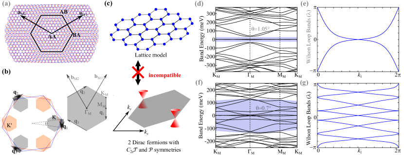
The moirépotential (Eq. 2) is invariant (up to a gauge transformation) under the translations , . The translation symmetry of the moirépotential is manifest in real space (Fig. 1a). The corresponding reciprocal lattice bases are , (Fig. 1b). The unit cell spanned by and is referred to as the moiréunit cell. Each moiréunit cell has one AA region, one AB region, and one BA region. In the AA region, the A(B) sublattice of the top layer sit on top of the A(B) sublattice of the bottom layer; in the AB region, the A and B sublattices of the top layer sit on top of the B sublattices and the empty hexagon centers of the bottom layer, respectively; in the BA region, the B and A sublattices of the upper layer sit on top of the A sublattices and the empty hexagon centers of the lower layer, respectively. First principle calculations show that the two layers are corrugated in the -direction Uchida et al. (2014); van Wijk et al. (2015); Dai et al. (2016); Jain et al. (2016). The distance between the two layers in the AA region is larger than the distance in the AB and BA regions. Since and are mainly dominated by the couplings in the AA and AB/BA regions Bistritzer and MacDonald (2011), respectively, this implies that, in the realistic model, is smaller than Koshino et al. (2018). In Figs. 1d and 1f, we show the the band structures for two different twist angles . The parameters are set as , , , .
II.2 Symmetries of the BM model
The model Eq. 1 has several point group symmetries: (i) , where is the complex conjugation, (ii) , (iii) . One can verify that the Hamiltonian is invariant under these symmetries. Notice that the single-graphene-valley Hamiltonian does not have the rotation and the time-reversal symmetries since they map one graphene valley to the other. The three crystalline symmetries and the moirétranslations generate the magnetic space group (#177.151 in the BNS setting Gallego et al. (2012)) Song et al. (2019).
We define a unitary particle-hole operation , which transforms the position as Song et al. (2019). Here are Pauli matrices representing the layer degree of freedom. Under the Hamiltonian transforms as
| (4) |
The second term on the right hand side is in linear order of . It approaches zero when . While the other terms in do not vanish in the limit. Thus it is safe to ignore this term in the small angle limit. To be specific, when , this term is of order and hence is much smaller than the energy scale of the low energy physics, which is of order . Therefore, is an emergent anticommuting symmetry when is small. It satisfies the algebra Song et al. (2019):
| (5) |
For later convenience, we define an anti-unitary particle operation , which is local in real space and satisfies . It acts on the Hamiltonian as
| (6) |
As discussed in details in Appendix B, the -dependence in the interlayer coupling may also cause a breaking of the emergent symmetry. We can also define a chiral operation , which is local in real space. Tarnopolsky et al. (2019). Under the Hamiltonian transforms as
| (7) |
In the so-called chiral limit Tarnopolsky et al. (2019), i.e., , the second term on the right hand of side vanishes and hence become an emergent anticommuting symmetry. The chiral symmetry satisfies the algebra
| (8) |
We numerically checked how much and are broken in the wavefunctions of the model Eq. 1. To be specific, we define the errors of the two symmetries in the two flat bands as
| (9) |
| (10) |
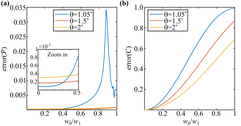
respectively, where and are the periodic parts of the Bloch states of the highest occupied band and the lowest empty band at charge neutrality, respectively, and is the area of the Moire Brillouin zone. When the two symmetries are exact, we have and hence the errors are zero. Using the parameters , , , we plot and as functions of (with fixed ) for a few twist angles in Fig. 2. For , is small () for , thus the symmetry is a good approximation for TBG, while the symmetry only starts being good (with error) for .
III Stable topology protected by particle-hole symmetry
III.1 The Wilson loop invariant protected by
We denote the Hamiltonian in momentum space as . We assume the emergent anti-unitary particle-hole symmetry, i.e., , and . As detailed in Section II.2, is anti-unitary and squares to -1, and is the product of the unitary of Ref. Song et al. (2019) and . We denote the energy and the periodic part of Bloch state of the -th band above (below) the zero energy as () and (), respectively. As explained in Appendix A and in Ref. Song et al. (2019), satisfies the periodicity , with being a reciprocal lattice and a unitary matrix referred to as the embedding matrix. Since anti-commutes with the Hamiltonian and flips the momentum, we have . The state must have the momentum and the energy . In general, is spanned by Bloch states at as
| (11) |
where the summation over is limited to those satisfying , and is a unitary matrix referred to as the sewing matrix of . is periodic in momentum space, i.e., Alexandradinata et al. (2016); Wang et al. (2016). Since , it should satisfy
| (12) |
Multiplying on the right hand side of the above equation, we obtain
| (13) |
We now prove that the symmetry protects a invariant for particle-hole symmetric separate bands, i.e., bands , gapped from higher and lower bands. This proof is not limited to TBG but applies to any system having our anti-unitary symmetry. We introduce the matrix . We parameterize as , where and are the reciprocal lattice basis vectors. Then we define the Wilson loop operator of the bands for a given as
| (14) |
The order of the matrices in the product is given by : matrices with larger () always appear on the right hand side of matrices with smaller . Due to the periodicity of Bloch states, is periodic.. Since is unitary, its eigenvalues are phase factors (), where ranges from to . are called as the Wilson loop bands. Topology is usually a result of Wilson loop flow, which in turn is a result of unavoidable crossings between Wilson loop bands.
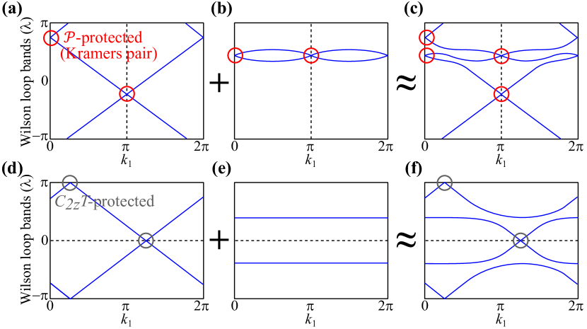
We now prove that the Wilson loop bands are doubly degenerate at and , as shown in Fig. 3a-c. In fact, we should heuristically expect this, since the Wilson loop respects as it contains all bands related by the particule-hole symmetry. Since is anti-unitary and squares to is hence acts as spinful time-reversal, which we already know to enforce Kramers doublets in the Wilson loop spectrum Yu et al. (2011); Alexandradinata et al. (2014). Due to Eq. 11, we have
| (15) |
In the above equation we have made use of a property of anti-unitary symmetries: for any two states , and an arbitrary anti-unitary operator , we have . Substituting this relation into Eq. 14 and using the periodicity relations and , we obtain
| (16) |
Since is periodic at , with are invariant under the particle-hole operation:
| (17) |
It is this invariance that protects degeneracies of Wilson loop bands at . To see this, we parameterize the unitary matrix as with being a hermitian matrix periodic in , called the Wilson Hamiltonian. The eigenvalues of form the Wilson loop bands. We can define the particle-hole operator for as such that Eq. 16 can be written as . We have due to Eq. 12. It is worth noting that unlike the Hamiltonian which anti-commutes with , commutes with . Because and for , the Wilson loop bands - the eigenstates of the Wilson Hamiltonian - at form doublets due to the Kramers theorem.
The invariant is defined such that if the Wilson loop bands form a zigzag flow between and - equivalent to a Quantum Spin Hall flow of Kramers paired Wannier centers, and otherwise. Examples of and with only symmetry are shown in Figs. 3a and 3b, respectively. Fig. 3a does not contain the symmetry and is meant to depict the possible cases with only our anti-unitary symmetry. Because the degeneracies at are protected by , a zigzag flow is stable against adding -preserving bands as long as these bands are topologically trivial (they do not exhibit Wilson loop flow themselves) that do not close the gaps between the bands and the higher/lower bands (Fig. 3a-c).
In Figs. 1e and 1g, we plot the Wilson loop bands of the middle two bands () of TBG with and the Wilson loop bands of the middle ten bands () of TBG with , respectively. Both have the zigzag flow and hence have . We do not plot the Wilson loop bands of the middle ten bands of TBG with because they have touching points with higher/lower bands at generic momenta (away from high symmetry lines).
III.2 Comparison of the -protected topology and -protected topology
In Ref. Song et al. (2019), some of the authors of the present work proved that the symmetry protects the Wilson loop flow for two bands, as shown in Fig. 3d, where the crossings at are protected by . The Wilson loop flow is characterized by an integer-valued invariant : the winding number of a smooth branch of the Wilson loop bands. There is a gauge ambiguity for the sign of . For example, the Wilson loop bands in Fig. 3d has if we choose the branch going up to define the winding number and if we choose the branch going down. is also referred to as the Euler’s class Ahn et al. (2019), as will be briefly introduced in Section V. With only symmetry, the flow can be broken by adding two trivial (flat) Wilson loop bands, as shown in Fig. 3d-f, since the crossings at generic positions - different from - in the Wilson loop spectrum are not protected by . After the Wilson loop bands are gapped, one can still define a -protected invariant through the nested Wilson loop Ahn et al. (2019); Song et al. (2019). Nevertheless, this -protected invariant does not correspond to Wannier obstruction Ahn et al. (2019); Po et al. (2019). Therefore, the topology protected only by is fragile. Ref. Song et al. (2019) showed that, by adding the unitary particle-hole symmetry , one cannot render the Stiefel–Whitney class Ahn et al. (2019) trivial by adding more bands; however, nontrivial Stiefel-Whitney index does not imply non-Wannierizable bands, and hence Song et al. (2019) called the index “stable”, between quotation marks; this paper removes the quotation marks by proving non-wannieralizability.
On the contrary, with the symmetry, we cannot break the zigzag flow by adding trivial (non-winding) Wilson loop bands, just like in the Quantum Spin Hall problem. First, due to the Kramers degeneracy guaranteed by , a trivial state must have at least two Wilson loop bands - corresponding to the fact that, with particle-hole symmetry, we must add to the nontrivial bands, generically, two bands - of some energy . The two Wilson loop bands are separated at generic but degenerate at , as shown in Fig. 3b. If we couple such a two-band trivial state to the topological state, the total Wilson loop bands are still gapless (Fig. 3c) since the degeneracies at are protected. Therefore, the topology protected by is stable.
If a two-band system has both and symmetries, the invariant protected by is given by the parity of , i.e., mod 2. For example, the Wilson loop bands in Fig. 1e has and . There is stable topology from , in systems with an even number of bands. TBG has even number of bands (as it has to, since implies even number of bands: nonzero energy states come in pairs , while zero energy states have Kramers degeneracy since ); furthermore, these bands exhibit () Dirac nodes at zero energy (proved in Section IV), which will show that TBG is in the topologically nontrivial class of this symmetry.
III.3 An alternative expression of the invariant
We have mentioned that the zigzag flow of the Wilson loop bands protected by is same as the zigzag flow of Wilson loop bands protected by the time-reversal symmetry in 2D Quantum Spin Hall topological insulator Yu et al. (2011). Now we show that they are indeed equivalent. Suppose have the () symmetry, i.e., , then we define the squared Hamiltonian as such that it commutes with , i.e., . We can regard as a “time-reversal symmetry” of . An eigenstate of with the energy is still an eigenstate of but has the squared energy . States of the particle-hole-symmetric bands used to define the Wilson loop (Eq. 14), i.e., , form the lowest bands of the squared Hamiltonian . Thus the Wilson loop operator of the particle-hole symmetric bands of is same as the Wilson loop operator of the lowest bands of . The zigzag flow of the Wilson loop can be equivalently thought as protected by the “time-reversal symmetry” of .
The time-reversal-protected invariant can be alternatively expressed as a topological obstruction Fu and Kane (2006); Fukui and Hatsugai (2007). Consider bands in a time-reversal () symmetric system that satisfy the gauge condition , , then the corresponding invariant is given by
| (18) |
where is half of the BZ whose boundary is -invariant,
| (19) |
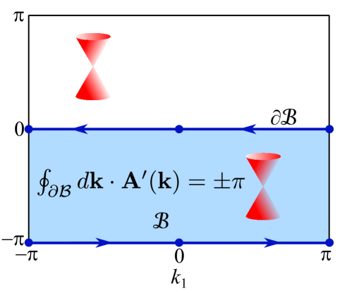
is the Berry’s connection of the considered bands, and is the Berry’s curvature. An example of is shown in Fig. 4. We regard as the lowest bands of and the “time-reversal symmetry” of . If we impose the gauge (), i.e., choose the sewing matrix defined in Eq. 11 as , then we can regard and as and , respectively. Thus the invariant of the bands of protected by is given by Eq. 18. This expression will be used for one of the ways to prove the symmetry anomaly of Dirac points in systems with and symmetries (See Section IV).
IV A no-go theorem of two Dirac fermions on lattices with and symmetries
In this section, we will prove that if there are () Dirac fermions at zero energy (chemical potential) in a system with and symmetries, then the invariant of the bands (arbitrary ) above and below the chemical potential, i.e., , is guaranteed to be 1, provided that the bands are gapped from other bands. As a consequence, for arbitrary , the particle-hole symmetric bands are not Wannierizable. That means the Dirac fermions do not have a lattice support.
Before going into a mathematical proof, we first give an intuitive proof that the Wilson loop of a and system with Dirac fermions at zero energy needs to wind. We first assume that we have bands separate from other bands close to charge neutrality. In Ahn et al. (2019); Xie et al. (2020a) it was shown that the number of Dirac points in half BZ equals the winding of the Wilson loop. For Dirac nodes in between these two bands, the winding would be odd, as in Fig. 1e. Adding non-zero trivial or nontrivial energy bands to this system would happen in pairs; introducing a set (trivial, due to , which renders Chern numbers to be zero and hence makes any single band topologically trivial) bands at non-zero energy would have its conjugate and appear in numbers . Introducing nontrivial bands at nonzero energy would mean introducing bands into the system, as any possible nontrivial set of bands at a given energy comes as a multiple of . These bands can introduce only a multiple of number of Dirac fermions into the system: each set of two separate bands has to have a multiple of Dirac fermions. From our Quantum Spin Hall (QSH) experience, whatever number of bands we introduce on top of our nontrivial bands with Dirac fermions cannot change the Wilson loop winding, as we are either adding trivial bands or pairs of nontrivial bands to a QSH system. Hence the winding (of the Dirac fermion band) is stable to the addition of any bands respecting and . The only way the winding can be interrupted is by the addition of one set of bands with Wilson loop winding to the already existent Wilson loop winding -bands. However, since with the number of Dirac nodes is equal to twice times the winding, this additional one set of -bands would bring about another Dirac points so the full system would have a number of Dirac fermions divisible by . Hence a system with Dirac fermions and and has to exhibit Wilson loop winding.
Now, by making use of Eq. 18, we give another proof that bands (gapped from other bands) with and symmetries that have Dirac points between and must have a nontrivial topology. Due to the symmetry, the Bloch states satisfy
| (20) |
where is unitary and called the sewing matrix. The summation over is limited to values satisfying . Substituting this constraint into the definition of the Berry’s curvature , we find that Ahn et al. (2019); Xie et al. (2020a); Bouhon et al. (2019). Thus we only need to evaluate the first term on the right hand side of Eq. 18. We define for the positive bands and for the negative bands. The total Berry’s connection is . By imposing the gauge condition () required by Eq. 18, we find
| (21) |
where we have applied the property of anti-unitary symmetry introduced below Eq. 15. Since the boundary (Fig. 4) is invariant under , the integrals of and are equal, i.e.,
| (22) |
The symmetry stabilizes 2D Dirac points Bernevig and Hughes (2013), and each Dirac point between the positive bands and the negative bands contribute to a or Berry’s phase of (Fig. 4). Due to the symmetry , the Dirac points must be equally distributed in and its complementary set BZ - . Hence if there are Dirac points in the BZ, there will be Dirac points in and we have mod . According to Eq. 22, we have
| (23) |
Substituting this equation into Eq. 18 and using the fact that , we obtain . Thus the presence of Dirac points in a system with and symmetries implies a nontrivial topology. In contrast to lattice models whose whole bands are trivial, this nontrivial topology is guaranteed by the Dirac points between and and hence cannot be trivialized by adding higher and lower energy bands (preserving ). Therefore, no matter how many high energy bands are included, as long as they respect and , the considered bands must have have nontrivial topology. As will be shown in next paragraph, in a lattice model with a finite number of orbitals per unit cell, the Wilson loop bands of the whole bands must be trivial. Therefore, Dirac points cannot be realized in lattice models because the corresponding band structure, no matter how many high and low energy bands are considered, must be topologically nontrivial.
Here we show that the whole bands of a lattice model must be trivial. Let the lattice model has orbitals, then the matrix entering the Wilson loop operator (Eq. 14) of the whole bands is . By the completeness of all the Bloch states we have . Thus the Wilson loop operator in Eq. 14 is , where is the embedding matrix defined in Appendix A (with ). Since is an unitary matrix, the eigenvalues of are same as eigenvalues of and hence do not change with and do not wind.
It is worth noting that, in TBG, the symmetry anomaly does not depend on the parameters of the Hamiltonian Eq. 1. In the weak coupling limit (, ), we have two Dirac points at and in the moiréBZ. If the bands are gapped from the other bands, the bands must be topological due to correspondence between the number of Dirac points and the invariant . Tuning the parameters of TBG may couple the bands to higher bands () and lower bands , which are assumed be gapped from and as we tune the parameters. In the weak coupling limit, the additional bands must have since they do not have Dirac points between and . Therefore, after we couple the bands to the bands, the bands as a whole will have . As we tune the parameters, additional Dirac points between and may be created due to gap closing and reopening between and . However, the total number of Dirac points between and must equal to 2 4, i.e., (), because the topological invariant of the bands is guaranteed to be .
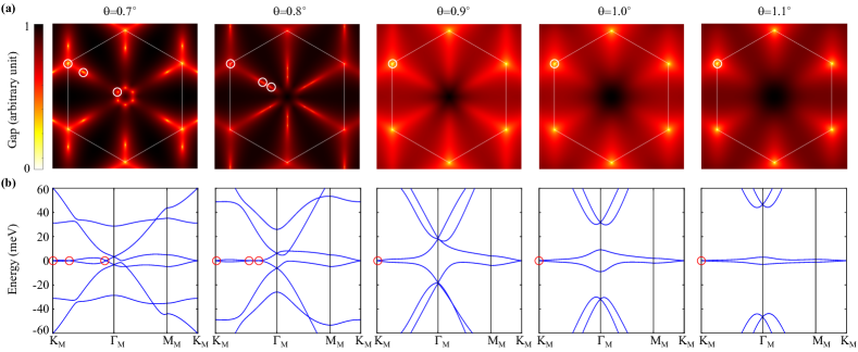
In Fig. 5, we show the evolution of Dirac points with the twisting angle changing from to . For , there are only two Dirac points in the moiréBrillouin zone and they locate at and , respectively. When decreases to , two additional Dirac points are generated along the high symmetry line . Due to the and symmetries, there are twelve Dirac points generated along the equivalent paths of . Thus for , there are in total fourteen Dirac points in the Brillouin zone. Therefore, we always have () Dirac points: for and for .
V The Chern band basis
In this section we show that, if the two bands and are gapped from other bands, we can recombine them as two Chern bands with Chern numbers and , with being the Euler’s class Ahn et al. (2019, 2018); Ünal et al. (2020); Wu et al. (2019b) (or, equivalently, the Wilson loop winding number protected by Xie et al. (2020a)). (In TBG, the Chern numbers given by are also equal to the index defined in Ref. Bernevig et al. (2020b), which, in a certain gauge, represents the eigenvalue of the Pauli matrix in the 2-dimensional space of band indices.)
In order to introduce the Chern band basis, we first introduce the definition of Euler’s class . (We refer the readers to Refs. [Ahn et al., 2019, Ahn et al., 2018, Xie et al., 2020a] for more details.) Suppose the two bands and are gapped from other bands. Then, at away from Dirac points between the two bands, the operator leaves each band unchanged up to a phase factor. In other words, the sewing matrix (Eq. 20) is diagonal at these . Hence in general, the symmetry acts on the Bloch states as (), with being the phase factors. According to Ref. Ahn et al. (2019), it follows that the non-Abelian Berry’s connection of the two bands at away from Dirac points takes the form
| (24) |
is a gauge invariant quantity up to a global ambiguity of sign. The Euler’s class is given by
| (25) |
Here indexes the Dirac points in the BZ, is a sufficiently small region covering the -th Dirac point, , and .
In the above we have assumed that the is smooth over the Brillouin zone except at the Dirac points. Eq. 24 is valid only in this gauge. In this gauge is necessarily k-dependent if there exist Dirac points between the th band and other bands. Since each Dirac point contributes to a Berry’s phase, there must be mod . Thus must wind odd times around a Dirac point.
We introduce the two Chern band basis as
| (26) |
There are two ambiguities in the above equation: (i) There is an ambiguity of the two branches of , i.e., and . (ii) At the Dirac points, where the two bands are degenerate, there is an ambiguity of choosing and . Replacing by or replacing by will interchange with . Similarly, interchanging and at the Dirac points will also interchange with at the Dirac points. To solve these ambiguities, as detailed in Appendix C, we require that the Berry’s curvatures of and to be continuous, or, equivalently,
| (27) |
where . Using Eqs. 24 and 26, we can calculate the non-Abelian Berry’s connection on the basis at away from the Dirac points. We obtain
| (28) |
and hence
| (29) |
for not at the Dirac points. Therefore, if the Berry’s curvature does not diverge at Dirac points, which is true as shown in next paragraph, the Chern numbers of the states are
| (30) |
To conclude this section, we show that in the chiral limit the Chern band basis can be chosen as the eigenstates of the chiral symmetry (Eq. 7). We define the sewing matrix of as
| (31) |
where the summation over satisfies . For the TBG Hamiltonian Eq. 1, the and operators are and , respectively. Thus we have the algebra and and hence
| (32) |
| (33) |
As discussed at the beginning of this section, at not at the Dirac points, we have . Then the solution of is
| (34) |
The sign cannot be determined by solving Eqs. 32 and 33. In practice, one should evaluate Eq. 31 to determine the sign for given . We find that the Chern band basis Eq. 26 diagonalizes . Below Eq. 26 we have discussed the ambiguity of choosing and we have imposed Eq. 27 to fix this ambiguity. This ambiguity of Eq. 26 can be alternatively solved by choosing as the eigenstates of with the eigenvalues , respectively. This choice automatically satisfies Eq. 27 since the states with different chiral eigenvalues are orthogonal, i.e., for arbitrary and .
VI Perfect metal phase of twisted bilayer graphene in the second chiral limit
In our article Ref. Bernevig et al. (2020b), we consider the opposite limit of the usual chiral limit: Instead of letting , we take to be zero. When , the model Eq. 1 has another chiral symmetry acting on the Hamiltonian as . Thus we call this limit as the second chiral limit. As discussed in Section II.1, and are the interlayer couplings contributed mainly by the AA and AB/BA regions, respectively; thus the second chiral limit can be (approximately) realized if the layer distance in the AA region is smaller than the layer distance in the AB and BA regions (shorter distance means stronger coupling). Such a configuration would be different from the corrugation predicted by the first principle calculations Uchida et al. (2014); van Wijk et al. (2015); Dai et al. (2016); Jain et al. (2016), where the distance in the AA region is larger. Nevertheless, the second chiral limit might could potentially be engineered by putting the TBG on certain substrate, and it represents an interesting interacting limit Bernevig et al. (2020b). We are mainly interested in the novel electronic band structure of TBG in the second chiral limit and hence we leave the material realization of the second chiral limit for future study.
We find that, in the second chiral limit, the -th positive (negative) band is always connected to the -th positive (negative) band. As the first positive band and the first negative band are connected through the Dirac points, the whole bands are all connected, as shown in Fig. 6a. The phase with all bands connected is referred to as the perfect metal Mora et al. (2019) in trilayer systems, where the number of Dirac nodes is odd. In the current case, we also find this “perfect metal” in even number of Dirac node systems with the special chiral symmetry of the second chiral limit.
The perfect metal phase is protected by , , and . The new chiral symmetry has a strange group algebra as it anticommutes with and with Lian et al. (2020b). We define the product of and as an effective inversion symmetry . It commutes with the Hamiltonian, i.e., and accordingly. The effective inversion operator satisfies the algebra
| (35) |
We first show that and protect double degeneracies at -invariant momenta. (In TBG, the -invariant momenta are and the three equivalent .) Since the Hamiltonian at an -invariant momentum commutes with , the Bloch states at this momentum must form eigenstates of . Suppose is such an eigenstate with eigenvalue 1, then we can show that must have the opposite eigenvalue -1 due to the anti-commutation between and . Therefore and form a doublet that has opposite eigenvalues. This explains the double degeneracies at and shown in Fig. 6a.
Next we prove that, for arbitrary even , the -th positive band is connected to the -th positive bands through () Dirac points. (For odd , we know by counting - see Fig. 6 - that the -th band is connected to the -th band through the double degeneracies at the -invariant momenta.) We only need to prove for the situation where the four bands , , , do not form four-fold degeneracies at high symmetry momenta since otherwise is already connected to . (As shown in Fig. 6a, we also do not observe four-fold degeneracies at high symmetry momenta.) We assume there are in total Dirac points between the first positive bands and the other bands. The Dirac points can appear above the -th band, i.e., between and , or below the first band, i.e., between and . According to the symmetry, half of the BZ () must have Dirac points. (The choice of is not unique. An example is shown in Fig. 4.) With the symmetry, the number of Dirac points in is related to the Berry’s phase surrounding as Bernevig and Hughes (2013)
| (36) |
where is the Berry’s connection of the first positive bands. In presence of the effective inversion symmetry , the right hand side of the above equation is determined by the eigenvalues as Fang et al. (2012); Hughes et al. (2011); Turner et al. (2012); Alexandradinata et al. (2014)
| (37) |
where indexes the four -invariant momenta, and is the eigenvalue of the -th positive band at the momentum . As discussed in the last paragraph, each doublet at an -invariant momentum has opposite eigenvalues. Thus, there are equal number of eigenvalues 1 and at the -invariant momenta; since the total number of states at the four -invariant momenta is , there are eigenvalues with and eigenvalues with . Hence the right hand side of Eq. 37 is 1 and we have mod . According to Eq. 36, the total number of Dirac points is a multiple of 4, i.e., mod 4. As we have proved in Section IV, there must be () Dirac points between and , then the number of Dirac points between and is with . Thus the -th positive band is always connected to the -th positive band through Dirac points. According to the particle-hole symmetry , the -th negative band is also connected to the -th negative band through Dirac points. Therefore, the whole set of bands in the system will be connected.
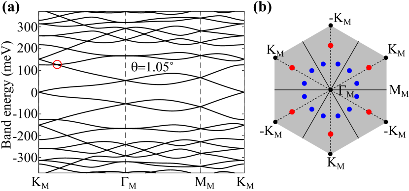
In general, the Dirac points between the -th band the -th band can be located anywhere in the BZ. However, with the and the symmetries of TBG, at least some of the Dirac points must locate at high symmetry point or along high symmetry lines of the BZ. We prove this statement by contradiction. The unitary point group of TBG is generated by , , and the effective inversion and hence is isomorphic to the point group , which has 12 elements in total. If all the Dirac points between the -th band the -th band are located at generic momenta, then the number of Dirac points would be a multiple of 12, as represented by the blue dots in Fig. 6b, leading to a contradictory with the Dirac points. Therefore, there must be 2 (modulo 4) Dirac points at the high symmetry points or along the high symmetry lines. As a consequence, the entire set of bands of TBG in the second chiral limit must be connected along the high symmetry lines. For example, as shown in Fig. 6a, there is a crossing between the 2nd and 3rd bands in the high symmetry line . (This crossing is protected by the effective mirror symmetry .) Under the actions of and , there are in total six symmetry counterparts of this crossing point (including itself). Thus the number of Dirac points is consistent with with .
VII Conclusions
In this work, we showed that even the simple, well studied BM TBG model still has several surprises related to the deep physics that it describes. We have proved that the band structure in a single graphene valley of TBG is anomalous, i.e., does not have lattice support that respects the and symmetries. The anomaly manifests as (i) a nontrivial topology protected of the bands for arbitrary , provided that the bands are gapped from other bands, (ii) () Dirac points between and . In the second chiral limit (), the anomaly manifests as (iii) a perfect metal phase where all the bands are connected.
As a consequence of the symmetry anomaly, a faithful description of TBG that respects all the symmetries of TBG, including , is forced to adopt a momentum space formalism. Any tight-binding description Po et al. (2019); Kang and Vafek (2018); Koshino et al. (2018); Bultinck et al. (2020a); Wilson et al. (2020) of TBG with finite number of orbitals must break at least one of the and symmetries (or the valley symmetry if the tight-binding model mix the two graphene valleys of TBG). In the other works of our series on TBG Bernevig et al. (2020a, b); Lian et al. (2020b); Bernevig et al. (2020c); Xie et al. (2020b), the interacting physics is studied using a momentum space formalism.
Acknowledgements.
We thank Aditya Cowsik and Fang Xie for valuable discussions. This work was supported by the DOE Grant No. DE-SC0016239, the Schmidt Fund for Innovative Research, Simons Investigator Grant No. 404513, the Packard Foundation, the Gordon and Betty Moore Foundation through Grant No. GBMF8685 towards the Princeton theory program, and a Guggenheim Fellowship from the John Simon Guggenheim Memorial Foundation. Further support was provided by the NSF-EAGER No. DMR 1643312, NSF-MRSEC No. DMR-1420541 and DMR-2011750, ONR No. N00014-20-1-2303, Gordon and Betty Moore Foundation through Grant GBMF8685 towards the Princeton theory program, BSF Israel US foundation No. 2018226, and the Princeton Global Network Funds.References
- Bistritzer and MacDonald (2011) Rafi Bistritzer and Allan H. MacDonald, “Moiré bands in twisted double-layer graphene,” Proceedings of the National Academy of Sciences 108, 12233–12237 (2011).
- Cao et al. (2018a) Yuan Cao, Valla Fatemi, Ahmet Demir, Shiang Fang, Spencer L. Tomarken, Jason Y. Luo, Javier D. Sanchez-Yamagishi, Kenji Watanabe, Takashi Taniguchi, Efthimios Kaxiras, Ray C. Ashoori, and Pablo Jarillo-Herrero, “Correlated insulator behaviour at half-filling in magic-angle graphene superlattices,” Nature 556, 80–84 (2018a).
- Efimkin and MacDonald (2018) Dmitry K. Efimkin and Allan H. MacDonald, “Helical network model for twisted bilayer graphene,” Phys. Rev. B 98, 035404 (2018).
- Xie et al. (2019) Yonglong Xie, Biao Lian, Berthold Jäck, Xiaomeng Liu, Cheng-Li Chiu, Kenji Watanabe, Takashi Taniguchi, B Andrei Bernevig, and Ali Yazdani, “Spectroscopic signatures of many-body correlations in magic-angle twisted bilayer graphene,” Nature 572, 101–105 (2019).
- Das et al. (2020) Ipsita Das, Xiaobo Lu, Jonah Herzog-Arbeitman, Zhi-Da Song, Kenji Watanabe, Takashi Taniguchi, B Andrei Bernevig, and Dmitri K Efetov, “Symmetry broken chern insulators and magic series of rashba-like landau level crossings in magic angle bilayer graphene,” arXiv preprint arXiv:2007.13390 (2020).
- Po et al. (2018a) Hoi Chun Po, Liujun Zou, Ashvin Vishwanath, and T. Senthil, “Origin of Mott Insulating Behavior and Superconductivity in Twisted Bilayer Graphene,” Physical Review X 8, 031089 (2018a).
- Dodaro et al. (2018) John F Dodaro, Steven A Kivelson, Yoni Schattner, Xiao-Qi Sun, and Chao Wang, “Phases of a phenomenological model of twisted bilayer graphene,” Physical Review B 98, 075154 (2018).
- Yuan and Fu (2018) Noah FQ Yuan and Liang Fu, “Model for the metal-insulator transition in graphene superlattices and beyond,” Physical Review B 98, 045103 (2018).
- Ochi et al. (2018) Masayuki Ochi, Mikito Koshino, and Kazuhiko Kuroki, “Possible correlated insulating states in magic-angle twisted bilayer graphene under strongly competing interactions,” Phys. Rev. B 98, 081102 (2018).
- Xu et al. (2018) Xiao Yan Xu, K. T. Law, and Patrick A. Lee, “Kekulé valence bond order in an extended hubbard model on the honeycomb lattice with possible applications to twisted bilayer graphene,” Phys. Rev. B 98, 121406 (2018).
- Venderbos and Fernandes (2018) Jörn W. F. Venderbos and Rafael M. Fernandes, “Correlations and electronic order in a two-orbital honeycomb lattice model for twisted bilayer graphene,” Phys. Rev. B 98, 245103 (2018).
- Kang and Vafek (2019) Jian Kang and Oskar Vafek, “Strong Coupling Phases of Partially Filled Twisted Bilayer Graphene Narrow Bands,” Physical Review Letters 122, 246401 (2019).
- Liu et al. (2019a) Jianpeng Liu, Zhen Ma, Jinhua Gao, and Xi Dai, “Quantum valley hall effect, orbital magnetism, and anomalous hall effect in twisted multilayer graphene systems,” Physical Review X 9, 031021 (2019a).
- Jiang et al. (2019) Yuhang Jiang, Xinyuan Lai, Kenji Watanabe, Takashi Taniguchi, Kristjan Haule, Jinhai Mao, and Eva Y. Andrei, “Charge order and broken rotational symmetry in magic-angle twisted bilayer graphene,” Nature 573, 91–95 (2019).
- Choi et al. (2019) Youngjoon Choi, Jeannette Kemmer, Yang Peng, Alex Thomson, Harpreet Arora, Robert Polski, Yiran Zhang, Hechen Ren, Jason Alicea, Gil Refael, and et al., “Electronic correlations in twisted bilayer graphene near the magic angle,” Nature Physics 15, 1174–1180 (2019).
- Polshyn et al. (2019) Hryhoriy Polshyn, Matthew Yankowitz, Shaowen Chen, Yuxuan Zhang, K. Watanabe, T. Taniguchi, Cory R. Dean, and Andrea F. Young, “Large linear-in-temperature resistivity in twisted bilayer graphene,” Nature Physics 15, 1011–1016 (2019).
- Pixley and Andrei (2019) Jed H. Pixley and Eva Y. Andrei, “Ferromagnetism in magic-angle graphene,” Science 365, 543–543 (2019), https://science.sciencemag.org/content/365/6453/543.full.pdf .
- Xie and MacDonald (2020a) Ming Xie and A. H. MacDonald, “Nature of the correlated insulator states in twisted bilayer graphene,” Phys. Rev. Lett. 124, 097601 (2020a).
- Bultinck et al. (2020a) Nick Bultinck, Eslam Khalaf, Shang Liu, Shubhayu Chatterjee, Ashvin Vishwanath, and Michael P. Zaletel, “Ground state and hidden symmetry of magic-angle graphene at even integer filling,” Phys. Rev. X 10, 031034 (2020a).
- Nuckolls et al. (2020) Kevin P. Nuckolls, Myungchul Oh, Dillon Wong, Biao Lian, Kenji Watanabe, Takashi Taniguchi, B. Andrei Bernevig, and Ali Yazdani, “Strongly Correlated Chern Insulators in Magic-Angle Twisted Bilayer Graphene,” arXiv e-prints , arXiv:2007.03810 (2020), arXiv:2007.03810 [cond-mat.mes-hall] .
- Wu et al. (2020) Shuang Wu, Zhenyuan Zhang, K. Watanabe, T. Taniguchi, and Eva Y. Andrei, “Chern Insulators and Topological Flat-bands in Magic-angle Twisted Bilayer Graphene,” arXiv e-prints , arXiv:2007.03735 (2020), arXiv:2007.03735 [cond-mat.mes-hall] .
- Saito et al. (2020) Yu Saito, Jingyuan Ge, Louk Rademaker, Kenji Watanabe, Takashi Taniguchi, Dmitry A. Abanin, and Andrea F. Young, “Hofstadter subband ferromagnetism and symmetry broken Chern insulators in twisted bilayer graphene,” arXiv e-prints , arXiv:2007.06115 (2020), arXiv:2007.06115 [cond-mat.mes-hall] .
- Wong et al. (2020) Dillon Wong, Kevin P. Nuckolls, Myungchul Oh, Biao Lian, Yonglong Xie, Sangjun Jeon, Kenji Watanabe, Takashi Taniguchi, B. Andrei Bernevig, and Ali Yazdani, “Cascade of electronic transitions in magic-angle twisted bilayer graphene,” Nature 582, 198–202 (2020).
- Zondiner et al. (2020) U. Zondiner, A. Rozen, D. Rodan-Legrain, Y. Cao, R. Queiroz, T. Taniguchi, K. Watanabe, Y. Oreg, F. von Oppen, Ady Stern, and et al., “Cascade of phase transitions and dirac revivals in magic-angle graphene,” Nature 582, 203–208 (2020).
- Sharpe et al. (2019) Aaron L. Sharpe, Eli J. Fox, Arthur W. Barnard, Joe Finney, Kenji Watanabe, Takashi Taniguchi, M. A. Kastner, and David Goldhaber-Gordon, “Emergent ferromagnetism near three-quarters filling in twisted bilayer graphene,” Science 365, 605–608 (2019).
- Serlin et al. (2019) M. Serlin, C. L. Tschirhart, H. Polshyn, Y. Zhang, J. Zhu, K. Watanabe, T. Taniguchi, L. Balents, and A. F. Young, “Intrinsic quantized anomalous hall effect in a moiré heterostructure,” Science 367, 900–903 (2019).
- Bultinck et al. (2020b) Nick Bultinck, Shubhayu Chatterjee, and Michael P. Zaletel, “Mechanism for anomalous hall ferromagnetism in twisted bilayer graphene,” Phys. Rev. Lett. 124, 166601 (2020b).
- Saito et al. (2020a) Yu Saito, Jingyuan Ge, Kenji Watanabe, Takashi Taniguchi, Erez Berg, and Andrea F. Young, “Isospin pomeranchuk effect and the entropy of collective excitations in twisted bilayer graphene,” (2020a), arXiv:2008.10830 [cond-mat.mes-hall] .
- Kang and Vafek (2020) Jian Kang and Oskar Vafek, “Non-abelian dirac node braiding and near-degeneracy of correlated phases at odd integer filling in magic-angle twisted bilayer graphene,” Phys. Rev. B 102, 035161 (2020).
- Soejima et al. (2020) Tomohiro Soejima, Daniel E. Parker, Nick Bultinck, Johannes Hauschild, and Michael P. Zaletel, “Efficient simulation of moire materials using the density matrix renormalization group,” (2020), arXiv:2009.02354 [cond-mat.str-el] .
- Cao et al. (2020a) Yuan Cao, Debanjan Chowdhury, Daniel Rodan-Legrain, Oriol Rubies-Bigorda, Kenji Watanabe, Takashi Taniguchi, T. Senthil, and Pablo Jarillo-Herrero, “Strange metal in magic-angle graphene with near planckian dissipation,” Phys. Rev. Lett. 124, 076801 (2020a).
- Kwan et al. (2020) Yves H. Kwan, Glenn Wagner, Nilotpal Chakraborty, Steven H. Simon, and S. A. Parameswaran, “Orbital chern insulator domain walls and chiral modes in twisted bilayer graphene,” (2020), arXiv:2007.07903 [cond-mat.str-el] .
- Cao et al. (2018b) Yuan Cao, Valla Fatemi, Shiang Fang, Kenji Watanabe, Takashi Taniguchi, Efthimios Kaxiras, and Pablo Jarillo-Herrero, “Unconventional superconductivity in magic-angle graphene superlattices,” Nature 556, 43–50 (2018b).
- Lu et al. (2019) Xiaobo Lu, Petr Stepanov, Wei Yang, Ming Xie, Mohammed Ali Aamir, Ipsita Das, Carles Urgell, Kenji Watanabe, Takashi Taniguchi, Guangyu Zhang, et al., “Superconductors, orbital magnets and correlated states in magic-angle bilayer graphene,” Nature 574, 653–657 (2019).
- Yankowitz et al. (2019) Matthew Yankowitz, Shaowen Chen, Hryhoriy Polshyn, Yuxuan Zhang, K Watanabe, T Taniguchi, David Graf, Andrea F Young, and Cory R Dean, “Tuning superconductivity in twisted bilayer graphene,” Science 363, 1059–1064 (2019).
- Wu et al. (2018) Fengcheng Wu, A. H. MacDonald, and Ivar Martin, “Theory of phonon-mediated superconductivity in twisted bilayer graphene,” Phys. Rev. Lett. 121, 257001 (2018).
- Xu and Balents (2018) Cenke Xu and Leon Balents, “Topological superconductivity in twisted multilayer graphene,” Physical review letters 121, 087001 (2018).
- Liu et al. (2018) Cheng-Cheng Liu, Li-Da Zhang, Wei-Qiang Chen, and Fan Yang, “Chiral spin density wave and d+ i d superconductivity in the magic-angle-twisted bilayer graphene,” Physical review letters 121, 217001 (2018).
- Isobe et al. (2018) Hiroki Isobe, Noah FQ Yuan, and Liang Fu, “Unconventional superconductivity and density waves in twisted bilayer graphene,” Physical Review X 8, 041041 (2018).
- Guinea and Walet (2018) Francisco Guinea and Niels R. Walet, “Electrostatic effects, band distortions, and superconductivity in twisted graphene bilayers,” Proceedings of the National Academy of Sciences 115, 13174–13179 (2018).
- Gonzalez and Stauber (2019) Jose Gonzalez and Tobias Stauber, “Kohn-luttinger superconductivity in twisted bilayer graphene,” Physical review letters 122, 026801 (2019).
- Lian et al. (2019) Biao Lian, Zhijun Wang, and B. Andrei Bernevig, “Twisted bilayer graphene: A phonon-driven superconductor,” Phys. Rev. Lett. 122, 257002 (2019).
- You and Vishwanath (2019) Y.-Z. You and A. Vishwanath, “Superconductivity from Valley Fluctuations and Approximate SO(4) Symmetry in a Weak Coupling Theory of Twisted Bilayer Graphene,” npj Quantum Materials 4, 16 (2019).
- Xie et al. (2020a) Fang Xie, Zhida Song, Biao Lian, and B. Andrei Bernevig, “Topology-bounded superfluid weight in twisted bilayer graphene,” Phys. Rev. Lett. 124, 167002 (2020a).
- Saito et al. (2020b) Yu Saito, Jingyuan Ge, Kenji Watanabe, Takashi Taniguchi, and Andrea F. Young, “Independent superconductors and correlated insulators in twisted bilayer graphene,” Nature Physics 16, 926–930 (2020b).
- Stepanov et al. (2020) Petr Stepanov, Ipsita Das, Xiaobo Lu, Ali Fahimniya, Kenji Watanabe, Takashi Taniguchi, Frank H. L. Koppens, Johannes Lischner, Leonid Levitov, and Dmitri K. Efetov, “Untying the insulating and superconducting orders in magic-angle graphene,” Nature 583, 375–378 (2020).
- Arora et al. (2020) Harpreet Singh Arora, Robert Polski, Yiran Zhang, Alex Thomson, Youngjoon Choi, Hyunjin Kim, Zhong Lin, Ilham Zaky Wilson, Xiaodong Xu, Jiun-Haw Chu, and et al., “Superconductivity in metallic twisted bilayer graphene stabilized by wse2,” Nature 583, 379–384 (2020).
- Khalaf et al. (2020) Eslam Khalaf, Shubhayu Chatterjee, Nick Bultinck, Michael P. Zaletel, and Ashvin Vishwanath, “Charged skyrmions and topological origin of superconductivity in magic angle graphene,” (2020), arXiv:2004.00638 [cond-mat.str-el] .
- Wu and Das Sarma (2020) Fengcheng Wu and Sankar Das Sarma, “Collective excitations of quantum anomalous hall ferromagnets in twisted bilayer graphene,” Physical Review Letters 124 (2020), 10.1103/physrevlett.124.046403.
- Julku et al. (2020) A. Julku, T. J. Peltonen, L. Liang, T. T. Heikkilä, and P. Törmä, “Superfluid weight and berezinskii-kosterlitz-thouless transition temperature of twisted bilayer graphene,” Physical Review B 101 (2020), 10.1103/physrevb.101.060505.
- König et al. (2020) E. J. König, Piers Coleman, and A. M. Tsvelik, “Spin magnetometry as a probe of stripe superconductivity in twisted bilayer graphene,” (2020), arXiv:2006.10684 [cond-mat.str-el] .
- Kang and Vafek (2018) Jian Kang and Oskar Vafek, “Symmetry, Maximally Localized Wannier States, and a Low-Energy Model for Twisted Bilayer Graphene Narrow Bands,” Phys. Rev. X 8, 031088 (2018).
- Koshino et al. (2018) Mikito Koshino, Noah F. Q. Yuan, Takashi Koretsune, Masayuki Ochi, Kazuhiko Kuroki, and Liang Fu, “Maximally localized wannier orbitals and the extended hubbard model for twisted bilayer graphene,” Phys. Rev. X 8, 031087 (2018).
- Ahn et al. (2019) Junyeong Ahn, Sungjoon Park, and Bohm-Jung Yang, “Failure of Nielsen-Ninomiya Theorem and Fragile Topology in Two-Dimensional Systems with Space-Time Inversion Symmetry: Application to Twisted Bilayer Graphene at Magic Angle,” Physical Review X 9, 021013 (2019).
- Po et al. (2019) Hoi Chun Po, Liujun Zou, T. Senthil, and Ashvin Vishwanath, “Faithful tight-binding models and fragile topology of magic-angle bilayer graphene,” Physical Review B 99, 195455 (2019).
- Song et al. (2019) Zhida Song, Zhijun Wang, Wujun Shi, Gang Li, Chen Fang, and B. Andrei Bernevig, “All Magic Angles in Twisted Bilayer Graphene are Topological,” Physical Review Letters 123, 036401 (2019).
- Liu et al. (2019b) Jianpeng Liu, Junwei Liu, and Xi Dai, “Pseudo landau level representation of twisted bilayer graphene: Band topology and implications on the correlated insulating phase,” Physical Review B 99, 155415 (2019b).
- Tarnopolsky et al. (2019) Grigory Tarnopolsky, Alex Jura Kruchkov, and Ashvin Vishwanath, “Origin of Magic Angles in Twisted Bilayer Graphene,” Physical Review Letters 122, 106405 (2019).
- Fu et al. (2018) Yixing Fu, E. J. König, J. H. Wilson, Yang-Zhi Chou, and J. H. Pixley, “Magic-angle semimetals,” (2018), arXiv:1809.04604 [cond-mat.str-el] .
- Zhang et al. (2019) Ya-Hui Zhang, Dan Mao, Yuan Cao, Pablo Jarillo-Herrero, and T Senthil, “Nearly flat chern bands in moiré superlattices,” Physical Review B 99, 075127 (2019).
- Lian et al. (2020a) Biao Lian, Fang Xie, and B. Andrei Bernevig, “Landau level of fragile topology,” Phys. Rev. B 102, 041402 (2020a).
- Lu et al. (2020) Xiaobo Lu, Biao Lian, Gaurav Chaudhary, Benjamin A. Piot, Giulio Romagnoli, Kenji Watanabe, Takashi Taniguchi, Martino Poggio, Allan H. MacDonald, B. Andrei Bernevig, and Dmitri K. Efetov, “Fingerprints of fragile topology in the hofstadter spectrum of twisted bilayer graphene close to the second magic angle,” (2020), arXiv:2006.13963 [cond-mat.mes-hall] .
- Padhi et al. (2020) Bikash Padhi, Apoorv Tiwari, Titus Neupert, and Shinsei Ryu, “Transport across twist angle domains in moiré graphene,” (2020), arXiv:2005.02406 [cond-mat.mes-hall] .
- Herzog-Arbeitman et al. (2020) Jonah Herzog-Arbeitman, Zhi-Da Song, Nicolas Regnault, and B. Andrei Bernevig, “Hofstadter Topology: Non-crystalline Topological Materials in the Moir\’e Era,” arXiv:2006.13938 [cond-mat] (2020), arXiv: 2006.13938.
- Wilson et al. (2020) Justin H. Wilson, Yixing Fu, S. Das Sarma, and J. H. Pixley, “Disorder in twisted bilayer graphene,” Phys. Rev. Research 2, 023325 (2020).
- Liu et al. (2020a) Xiaoxue Liu, Zhi Wang, K Watanabe, T Taniguchi, Oskar Vafek, and JIA Li, “Tuning electron correlation in magic-angle twisted bilayer graphene using coulomb screening,” arXiv preprint arXiv:2003.11072 (2020a).
- Kerelsky et al. (2019) Alexander Kerelsky, Leo J. McGilly, Dante M. Kennes, Lede Xian, Matthew Yankowitz, Shaowen Chen, K. Watanabe, T. Taniguchi, James Hone, Cory Dean, and et al., “Maximized electron interactions at the magic angle in twisted bilayer graphene,” Nature 572, 95–100 (2019).
- Choi et al. (2020) Youngjoon Choi, Hyunjin Kim, Yang Peng, Alex Thomson, Cyprian Lewandowski, Robert Polski, Yiran Zhang, Harpreet Singh Arora, Kenji Watanabe, Takashi Taniguchi, Jason Alicea, and Stevan Nadj-Perge, “Tracing out correlated chern insulators in magic angle twisted bilayer graphene,” (2020), arXiv:2008.11746 [cond-mat.str-el] .
- Park et al. (2020) Jeong Min Park, Yuan Cao, Kenji Watanabe, Takashi Taniguchi, and Pablo Jarillo-Herrero, “Flavour hund’s coupling, correlated chern gaps, and diffusivity in moiré flat bands,” (2020), arXiv:2008.12296 [cond-mat.mes-hall] .
- Rozen et al. (2020) Asaf Rozen, Jeong Min Park, Uri Zondiner, Yuan Cao, Daniel Rodan-Legrain, Takashi Taniguchi, Kenji Watanabe, Yuval Oreg, Ady Stern, Erez Berg, Pablo Jarillo-Herrero, and Shahal Ilani, “Entropic evidence for a pomeranchuk effect in magic angle graphene,” (2020), arXiv:2009.01836 [cond-mat.mes-hall] .
- Burg et al. (2019) G. William Burg, Jihang Zhu, Takashi Taniguchi, Kenji Watanabe, Allan H. MacDonald, and Emanuel Tutuc, “Correlated insulating states in twisted double bilayer graphene,” Phys. Rev. Lett. 123, 197702 (2019).
- Shen et al. (2020) Cheng Shen, Yanbang Chu, QuanSheng Wu, Na Li, Shuopei Wang, Yanchong Zhao, Jian Tang, Jieying Liu, Jinpeng Tian, Kenji Watanabe, Takashi Taniguchi, Rong Yang, Zi Yang Meng, Dongxia Shi, Oleg V. Yazyev, and Guangyu Zhang, “Correlated states in twisted double bilayer graphene,” Nature Physics 16, 520–525 (2020).
- Cao et al. (2020b) Yuan Cao, Daniel Rodan-Legrain, Oriol Rubies-Bigorda, Jeong Min Park, Kenji Watanabe, Takashi Taniguchi, and Pablo Jarillo-Herrero, “Tunable correlated states and spin-polarized phases in twisted bilayer–bilayer graphene,” Nature , 1–6 (2020b).
- Liu et al. (2019c) Xiaomeng Liu, Zeyu Hao, Eslam Khalaf, Jong Yeon Lee, Kenji Watanabe, Takashi Taniguchi, Ashvin Vishwanath, and Philip Kim, “Spin-polarized Correlated Insulator and Superconductor in Twisted Double Bilayer Graphene,” arXiv:1903.08130 [cond-mat] (2019c), arXiv: 1903.08130.
- Chen et al. (2019a) Guorui Chen, Lili Jiang, Shuang Wu, Bosai Lyu, Hongyuan Li, Bheema Lingam Chittari, Kenji Watanabe, Takashi Taniguchi, Zhiwen Shi, Jeil Jung, Yuanbo Zhang, and Feng Wang, “Evidence of a gate-tunable Mott insulator in a trilayer graphene moiré superlattice,” Nature Physics 15, 237 (2019a).
- Chen et al. (2019b) Guorui Chen, Aaron L. Sharpe, Patrick Gallagher, Ilan T. Rosen, Eli J. Fox, Lili Jiang, Bosai Lyu, Hongyuan Li, Kenji Watanabe, Takashi Taniguchi, Jeil Jung, Zhiwen Shi, David Goldhaber-Gordon, Yuanbo Zhang, and Feng Wang, “Signatures of tunable superconductivity in a trilayer graphene moiré superlattice,” Nature 572, 215–219 (2019b).
- Chen et al. (2020) Guorui Chen, Aaron L. Sharpe, Eli J. Fox, Ya-Hui Zhang, Shaoxin Wang, Lili Jiang, Bosai Lyu, Hongyuan Li, Kenji Watanabe, Takashi Taniguchi, Zhiwen Shi, T. Senthil, David Goldhaber-Gordon, Yuanbo Zhang, and Feng Wang, “Tunable correlated Chern insulator and ferromagnetism in a moiré superlattice,” Nature 579, 56–61 (2020).
- Burg et al. (2020) G. William Burg, Biao Lian, Takashi Taniguchi, Kenji Watanabe, B. Andrei Bernevig, and Emanuel Tutuc, “Evidence of emergent symmetry and valley chern number in twisted double-bilayer graphene,” (2020), arXiv:2006.14000 [cond-mat.mes-hall] .
- Zou et al. (2018) Liujun Zou, Hoi Chun Po, Ashvin Vishwanath, and T. Senthil, “Band structure of twisted bilayer graphene: Emergent symmetries, commensurate approximants, and wannier obstructions,” Phys. Rev. B 98, 085435 (2018).
- Bouhon et al. (2019) Adrien Bouhon, Annica M. Black-Schaffer, and Robert-Jan Slager, “Wilson loop approach to fragile topology of split elementary band representations and topological crystalline insulators with time-reversal symmetry,” Phys. Rev. B 100, 195135 (2019).
- Hejazi et al. (2019a) Kasra Hejazi, Chunxiao Liu, Hassan Shapourian, Xiao Chen, and Leon Balents, “Multiple topological transitions in twisted bilayer graphene near the first magic angle,” Phys. Rev. B 99, 035111 (2019a).
- Hejazi et al. (2019b) Kasra Hejazi, Chunxiao Liu, and Leon Balents, “Landau levels in twisted bilayer graphene and semiclassical orbits,” Physical Review B 100 (2019b), 10.1103/physrevb.100.035115.
- Wu et al. (2019a) Xiao-Chuan Wu, Chao-Ming Jian, and Cenke Xu, “Coupled-wire description of the correlated physics in twisted bilayer graphene,” Physical Review B 99 (2019a), 10.1103/physrevb.99.161405.
- Thomson et al. (2018) Alex Thomson, Shubhayu Chatterjee, Subir Sachdev, and Mathias S. Scheurer, “Triangular antiferromagnetism on the honeycomb lattice of twisted bilayer graphene,” Physical Review B 98 (2018), 10.1103/physrevb.98.075109.
- Seo et al. (2019) Kangjun Seo, Valeri N. Kotov, and Bruno Uchoa, “Ferromagnetic mott state in twisted graphene bilayers at the magic angle,” Phys. Rev. Lett. 122, 246402 (2019).
- Hejazi et al. (2020) Kasra Hejazi, Xiao Chen, and Leon Balents, “Hybrid wannier chern bands in magic angle twisted bilayer graphene and the quantized anomalous hall effect,” (2020), arXiv:2007.00134 [cond-mat.mes-hall] .
- Hu et al. (2019) Xiang Hu, Timo Hyart, Dmitry I. Pikulin, and Enrico Rossi, “Geometric and conventional contribution to the superfluid weight in twisted bilayer graphene,” Phys. Rev. Lett. 123, 237002 (2019).
- Christos et al. (2020) Maine Christos, Subir Sachdev, and Mathias Scheurer, “Superconductivity, correlated insulators, and wess-zumino-witten terms in twisted bilayer graphene,” (2020), arXiv:2007.00007 [cond-mat.str-el] .
- Lewandowski et al. (2020) Cyprian Lewandowski, Debanjan Chowdhury, and Jonathan Ruhman, “Pairing in magic-angle twisted bilayer graphene: role of phonon and plasmon umklapp,” (2020), arXiv:2007.15002 [cond-mat.supr-con] .
- Xie and MacDonald (2020b) Ming Xie and A. H. MacDonald, “Nature of the correlated insulator states in twisted bilayer graphene,” Phys. Rev. Lett. 124, 097601 (2020b).
- Liu and Dai (2020) Jianpeng Liu and Xi Dai, “Theories for the correlated insulating states and quantum anomalous hall phenomena in twisted bilayer graphene,” (2020), arXiv:1911.03760 [cond-mat.str-el] .
- Cea and Guinea (2020) Tommaso Cea and Francisco Guinea, “Band structure and insulating states driven by coulomb interaction in twisted bilayer graphene,” Phys. Rev. B 102, 045107 (2020).
- Zhang et al. (2020) Yi Zhang, Kun Jiang, Ziqiang Wang, and Fuchun Zhang, “Correlated insulating phases of twisted bilayer graphene at commensurate filling fractions: A hartree-fock study,” Phys. Rev. B 102, 035136 (2020).
- Liu et al. (2020b) Shang Liu, Eslam Khalaf, Jong Yeon Lee, and Ashvin Vishwanath, “Nematic topological semimetal and insulator in magic angle bilayer graphene at charge neutrality,” (2020b), arXiv:1905.07409 [cond-mat.str-el] .
- Da Liao et al. (2019) Yuan Da Liao, Zi Yang Meng, and Xiao Yan Xu, “Valence bond orders at charge neutrality in a possible two-orbital extended hubbard model for twisted bilayer graphene,” Phys. Rev. Lett. 123, 157601 (2019).
- Liao et al. (2020) Yuan Da Liao, Jian Kang, Clara N. Breiø, Xiao Yan Xu, Han-Qing Wu, Brian M. Andersen, Rafael M. Fernandes, and Zi Yang Meng, “Correlation-induced insulating topological phases at charge neutrality in twisted bilayer graphene,” (2020), arXiv:2004.12536 [cond-mat.str-el] .
- Classen et al. (2019) Laura Classen, Carsten Honerkamp, and Michael M Scherer, “Competing phases of interacting electrons on triangular lattices in moiré heterostructures,” Physical Review B 99, 195120 (2019).
- Kennes et al. (2018) Dante M Kennes, Johannes Lischner, and Christoph Karrasch, “Strong correlations and d+ id superconductivity in twisted bilayer graphene,” Physical Review B 98, 241407 (2018).
- Eugenio and Dağ (2020) P Myles Eugenio and Ceren B Dağ, “Dmrg study of strongly interacting flatbands: a toy model inspired by twisted bilayer graphene,” arXiv preprint arXiv:2004.10363 (2020).
- Huang et al. (2020) Yixuan Huang, Pavan Hosur, and Hridis K Pal, “Deconstructing magic-angle physics in twisted bilayer graphene with a two-leg ladder model,” arXiv preprint arXiv:2004.10325 (2020).
- Huang et al. (2019) Tongyun Huang, Lufeng Zhang, and Tianxing Ma, “Antiferromagnetically ordered mott insulator and d+ id superconductivity in twisted bilayer graphene: A quantum monte carlo study,” Science Bulletin 64, 310–314 (2019).
- Guo et al. (2018) Huaiming Guo, Xingchuan Zhu, Shiping Feng, and Richard T Scalettar, “Pairing symmetry of interacting fermions on a twisted bilayer graphene superlattice,” Physical Review B 97, 235453 (2018).
- Ledwith et al. (2020) Patrick J. Ledwith, Grigory Tarnopolsky, Eslam Khalaf, and Ashvin Vishwanath, “Fractional chern insulator states in twisted bilayer graphene: An analytical approach,” Phys. Rev. Research 2, 023237 (2020).
- Repellin et al. (2020) Cécile Repellin, Zhihuan Dong, Ya-Hui Zhang, and T. Senthil, “Ferromagnetism in narrow bands of moiré superlattices,” Phys. Rev. Lett. 124, 187601 (2020).
- Abouelkomsan et al. (2020) Ahmed Abouelkomsan, Zhao Liu, and Emil J. Bergholtz, “Particle-hole duality, emergent fermi liquids, and fractional chern insulators in moiré flatbands,” Phys. Rev. Lett. 124, 106803 (2020).
- Repellin and Senthil (2020) Cécile Repellin and T. Senthil, “Chern bands of twisted bilayer graphene: Fractional chern insulators and spin phase transition,” Phys. Rev. Research 2, 023238 (2020).
- Vafek and Kang (2020) Oskar Vafek and Jian Kang, “Towards the hidden symmetry in coulomb interacting twisted bilayer graphene: renormalization group approach,” (2020), arXiv:2009.09413 [cond-mat.str-el] .
- Fernandes and Venderbos (2020) Rafael M. Fernandes and Jörn W. F. Venderbos, “Nematicity with a twist: Rotational symmetry breaking in a moiré superlattice,” Science Advances 6 (2020), 10.1126/sciadv.aba8834, https://advances.sciencemag.org/content/6/32/eaba8834.full.pdf .
- Wang et al. (2020) Jie Wang, Yunqin Zheng, Andrew J. Millis, and Jennifer Cano, “Chiral approximation to twisted bilayer graphene: Exact intra-valley inversion symmetry, nodal structure and implications for higher magic angles,” (2020), arXiv:2010.03589 [cond-mat.mes-hall] .
- Bernevig et al. (2020a) B. Andrei Bernevig, Zhida Song, Nicolas Regnault, and Biao Lian, “TBG I: Matrix elements, approximations, perturbation theory and a 2-band model for twisted bilayer graphene,” arXiv e-prints , arXiv:2009.11301 (2020a), arXiv:2009.11301 .
- Bernevig et al. (2020b) B. Andrei Bernevig, Zhida Song, Nicolas Regnault, and Biao Lian, “TBG III: Interacting hamiltonian and exact symmetries of twisted bilayer graphene,” arXiv e-prints , arXiv:2009.12376 (2020b), arXiv:2009.12376 .
- Lian et al. (2020b) Biao Lian, Zhi-Da Song, Nicolas Regnault, Dmitri K. Efetov, Ali Yazdani, and B. Andrei Bernevig, “Tbg iv: Exact insulator ground states and phase diagram of twisted bilayer graphene,” arXiv e-prints , arXiv:2009.13530 (2020b), arXiv:2009.13530 .
- Bernevig et al. (2020c) B. Andrei Bernevig, Biao Lian, Aditya Cowsik, Fang Xie, Nicolas Regnault, and Zhi-Da Song, “TBG V: Exact analytic many-body excitations in twisted bilayer graphene coulomb hamiltonians: Charge gap, goldstone modes and absence of cooper pairing,” arXiv e-prints , arXiv:2009.14200 (2020c), arXiv:2009.14200 .
- Xie et al. (2020b) Fang Xie, Aditya Cowsik, Zhida Son, Biao Lian, B. Andrei Bernevig, and Nicolas Regnault, “TBG VI: An exact diagonalization study of twisted bilayer graphene at non-zero integer fillings,” arXiv e-prints , arXiv:2010.00588 (2020b), arXiv:2010.00588 .
- Po et al. (2018b) Hoi Chun Po, Haruki Watanabe, and Ashvin Vishwanath, “Fragile Topology and Wannier Obstructions,” Physical Review Letters 121, 126402 (2018b).
- Cano et al. (2018) Jennifer Cano, Barry Bradlyn, Zhijun Wang, L. Elcoro, M. G. Vergniory, C. Felser, M. I. Aroyo, and B. Andrei Bernevig, “Topology of disconnected elementary band representations,” Phys. Rev. Lett. 120, 266401 (2018).
- Else et al. (2019) Dominic V. Else, Hoi Chun Po, and Haruki Watanabe, “Fragile topological phases in interacting systems,” Phys. Rev. B 99, 125122 (2019).
- Mañes (2020) Juan L. Mañes, “Fragile phonon topology on the honeycomb lattice with time-reversal symmetry,” Phys. Rev. B 102, 024307 (2020).
- Alexandradinata et al. (2020) A. Alexandradinata, J. Höller, Chong Wang, Hengbin Cheng, and Ling Lu, “Crystallographic splitting theorem for band representations and fragile topological photonic crystals,” Phys. Rev. B 102, 115117 (2020).
- Uchida et al. (2014) Kazuyuki Uchida, Shinnosuke Furuya, Jun-Ichi Iwata, and Atsushi Oshiyama, “Atomic corrugation and electron localization due to moiré patterns in twisted bilayer graphenes,” Phys. Rev. B 90, 155451 (2014).
- van Wijk et al. (2015) M M van Wijk, A Schuring, M I Katsnelson, and A Fasolino, “Relaxation of moiré patterns for slightly misaligned identical lattices: graphene on graphite,” 2D Materials 2, 034010 (2015).
- Dai et al. (2016) Shuyang Dai, Yang Xiang, and David J Srolovitz, “Twisted bilayer graphene: Moiré with a twist,” Nano letters 16, 5923–5927 (2016).
- Jain et al. (2016) Sandeep K Jain, Vladimir Juričić, and Gerard T Barkema, “Structure of twisted and buckled bilayer graphene,” 2D Materials 4, 015018 (2016).
- Gallego et al. (2012) Samuel V Gallego, Emre S Tasci, G Flor, J Manuel Perez-Mato, and Mois I Aroyo, “Magnetic symmetry in the bilbao crystallographic server: a computer program to provide systematic absences of magnetic neutron diffraction,” Journal of Applied Crystallography 45, 1236–1247 (2012).
- Alexandradinata et al. (2016) A Alexandradinata, Zhijun Wang, and B Andrei Bernevig, “Topological insulators from group cohomology,” Physical Review X 6, 021008 (2016).
- Wang et al. (2016) Zhijun Wang, Aris Alexandradinata, Robert J Cava, and B Andrei Bernevig, “Hourglass fermions,” Nature 532, 189–194 (2016).
- Yu et al. (2011) Rui Yu, Xiao Liang Qi, Andrei Bernevig, Zhong Fang, and Xi Dai, “Equivalent expression of $\mathbbZ_2$ topological invariant for band insulators using the non-Abelian Berry connection,” Phys. Rev. B 84, 075119 (2011).
- Alexandradinata et al. (2014) A. Alexandradinata, Xi Dai, and B. Andrei Bernevig, “Wilson-loop characterization of inversion-symmetric topological insulators,” Phys. Rev. B 89, 155114 (2014).
- Fu and Kane (2006) Liang Fu and C. L. Kane, “Time reversal polarization and a adiabatic spin pump,” Phys. Rev. B 74, 195312 (2006).
- Fukui and Hatsugai (2007) Takahiro Fukui and Yasuhiro Hatsugai, “Quantum spin hall effect in three dimensional materials: Lattice computation of z2 topological invariants and its application to bi and sb,” Journal of the Physical Society of Japan 76, 053702–053702 (2007).
- Bernevig and Hughes (2013) B. Andrei Bernevig and Taylor L. Hughes, Topological Insulators and Topological Superconductors (Princeton University Press, 2013).
- Ahn et al. (2018) Junyeong Ahn, Dongwook Kim, Youngkuk Kim, and Bohm-Jung Yang, “Band Topology and Linking Structure of Nodal Line Semimetals with ${Z}_{2}$ Monopole Charges,” Physical Review Letters 121, 106403 (2018).
- Ünal et al. (2020) F. Nur Ünal, Adrien Bouhon, and Robert-Jan Slager, “Topological euler class as a dynamical observable in optical lattices,” Phys. Rev. Lett. 125, 053601 (2020).
- Wu et al. (2019b) QuanSheng Wu, Alexey A Soluyanov, and Tomáš Bzdušek, “Non-abelian band topology in noninteracting metals,” Science 365, 1273–1277 (2019b).
- Mora et al. (2019) Christophe Mora, Nicolas Regnault, and B. Andrei Bernevig, “Flatbands and perfect metal in trilayer moiré graphene,” Phys. Rev. Lett. 123, 026402 (2019).
- Fang et al. (2012) Chen Fang, Matthew J. Gilbert, and B. Andrei Bernevig, “Bulk topological invariants in noninteracting point group symmetric insulators,” Phys. Rev. B 86, 115112 (2012).
- Hughes et al. (2011) Taylor L. Hughes, Emil Prodan, and B. Andrei Bernevig, “Inversion-symmetric topological insulators,” Phys. Rev. B 83, 245132 (2011).
- Turner et al. (2012) Ari M. Turner, Yi Zhang, Roger S. K. Mong, and Ashvin Vishwanath, “Quantized response and topology of magnetic insulators with inversion symmetry,” Phys. Rev. B 85, 165120 (2012).
- Nam and Koshino (2017) Nguyen N. T. Nam and Mikito Koshino, “Lattice relaxation and energy band modulation in twisted bilayer graphene,” Phys. Rev. B 96, 075311 (2017).
- Koshino and Nam (2020) Mikito Koshino and Nguyen N. T. Nam, “Effective continuum model for relaxed twisted bilayer graphene and moiré electron-phonon interaction,” Phys. Rev. B 101, 195425 (2020).
- Fang et al. (2019) Shiang Fang, Stephen Carr, Ziyan Zhu, Daniel Massatt, and Efthimios Kaxiras, “Angle-dependent ab-initio low-energy hamiltonians for a relaxed twisted bilayer graphene heterostructure,” arXiv preprint arXiv:1908.00058 (2019).
Appendix A Hamiltonian of twisted bilayer graphene in momentum space
A.1 The Hamiltonian
Here we briefly introduce the momentum space Hamiltonian corresponding to Eq. 1. Readers may refer to the supplementary materials of Ref. Song et al. (2019) for more details. The basis of is , where is a momentum in the moiréBZ, is a point in the lattice shown in Fig. 7, and is the sublattice index of graphene. There are two types of lattices: the blue lattice and the red lattice . For , the basis is a plane-wave state from the top layer
| (38) |
where is the number of lattices in the top layer graphene, indexes all the lattices of the top layer graphene, is the sublattice vector of the top layer graphene, is the atomic orbital at . For , the basis is a plane-wave state from the bottom layer
| (39) |
where is the number of lattices in the bottom layer graphene (same as the one in top layer), indexes all the lattices of the bottom layer graphene, is the sublattice vector of the top layer graphene, is the atomic orbital at . The Hamiltonian (Eq. 1) on the basis is given by
| (40) |
where and () are two-by-two matrices in the sublattice space, for and for .

A.2 The periodicity of Bloch states
An eigenstate of Eq. 1 at a given momentum can be written as linear combination of the Bloch basis as . Here is the band index. It should be noticed that the basis states in Eqs. 38 and 39 are not periodic in the moiréBZ since by definition. In order for the Bloch state to be periodic in the moiréBZ, i.e., , should satisfy . We introduce the embedding matrix
| (41) |
such that we can write the periodicity of Bloch states as
| (42) |
where . While exact Bloch periodicity requires that the cutoff in the lattice be large, we have showed - around the first magic angle - Bernevig et al. (2020a) that we can obtain machine precision accuracy in the first moiréBZ by taking a small cutoff in
A.3 Symmetry operators in the momentum space
The crystalline symmetry group of the single valley Hamiltonian is the magnetic space group (#177.151 in the BNS setting Gallego et al. (2012)). The generators of this group are: The symmetry
| (43) |
where . The symmetry
| (44) |
where , and . The symmetry
| (45) |
where . It should be noticed that all rotations of momenta here are with respect to the point of the moiréBZ.
When the second term in Eq. 40 is negligible, has an emergent unitary particle-hole symmetry
| (46) |
where , and for and for . The anti-unitary particle-hole symmetry in momentum space is
| (47) |
where . When , has an emergent chiral symmetry
| (48) |
where . When , has an another emergent chiral symmetry (the second chiral symmetry)
| (49) |
where .
The embedding matrix transform under the unitary operators () as
| (50) |
For the unitary operator , we have
| (51) |
One can verify that the two identities by explicitly acting the symmetry operators on the embedding matrix.
A.4 The sewing matrices of symmetry operators
For the unitary crystalline symmetries, e.g., , we define the sewing matrices as
| (52) |
For the anti-unitary symmetries, e.g., , we define the sewing matrices as
| (53) |
Using the identities Eqs. 50 and 51, we obtain that the sewing matrices are periodic in momentum space, i.e., for arbitrary reciprocal lattice . The explicit expression for the sewing matrices depend on different basis, and will be give in Ref. Bernevig et al. (2020b) for the cases needed for our interacting problem.
Appendix B More discussions on the particle-hole symmetry
B.1 Effect of in-plane lattice relaxation
We first show that the in-plane relaxation does not directly lead to the particle-hole symmetry breaking. In Ref. Nam and Koshino (2017), Koshino et al. obtained the relaxed lattice structure of TBG by minimizing the elastic energy. The in-plane displacement of atoms in the two layers can be approximated as
| (54) |
where is the layer index and
| (55) |
is an odd function of and is dominated by the components on the shortest vectors Koshino and Nam (2020). For example, for , takes the form Koshino and Nam (2020)
| (56) |
where is the length of the displacement vectors. The in-plane displacement leads to two new terms in the Hamiltonian of TBG: (i) the correction of the intralayer hopping, which has a form of pseudo vector potential, (ii) the correction to the interlayer hopping. The pseudo vector potential has the form
| (57) |
with being the strain tensor and the coupling constant. Since is real and odd in , is real and even in . The pseudo vector potential enters the TBG Hamiltonian as
| (58) |
The factor in the pseudo vector potential term comes from the fact (Eq. 54). We find that the pseudo vector potential term respects all the symmetries. In particular, it respects the and the symmetries, which protect the stable topology.
With the in-plane displacement fields, the interlayer coupling changes to Koshino and Nam (2020)
| (59) |
where is the vector shown in Fig. 7, , , and are given in Eq. 3. The corresponding Hamiltonian matrix can be written as
| (60) |
with and being the real part and imaginary part of , respectively. Since is odd in , there is and . One can find that the interlayer coupling respects both and .
B.2 -dependence in the interlayer hopping
The continuous models of TBG discussed in the rest of this work have made an approximation on the interlayer coupling: We have neglected the -dependence of the Fourier transformation of the interlayer hopping. Refs. Koshino and Nam (2020) and Fang et al. (2019) have shown that keeping the -dependence in will lead to a particle-hole asymmetry in the energy spectrum. Ref. Fang et al. (2019) shows that keeping linear order of in the -dependence is a good approximation. Here we derive the linear -dependence explicitly. Following Eq. (14) of the supplementary material of Ref. Song et al. (2019), we have the intervalley coupling on the basis Eqs. 38 and 39
| (61) |
where is the Fourier transformation of the interlayer coupling with being the distance between the two layers, and
| (62) |
Here is the vector shown in Fig. 7, , . The parameters in have been fitted as , , , For simplicity here we assume is uniform in real space.
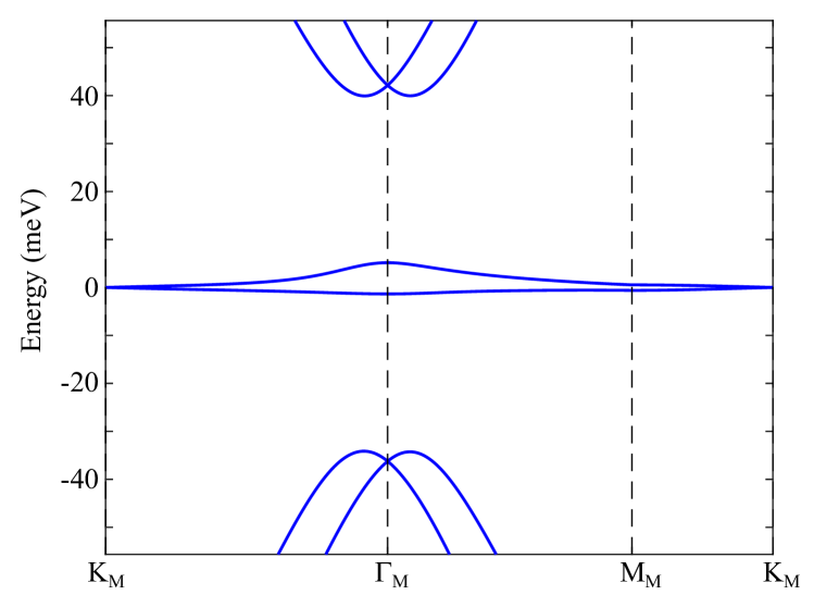
We expand to leading order of as
| (63) |
Then we obtain the correction to the continuous model as
| (64) |
for , and
| (65) |
for . Here . Since still consists of , , , it respects the symmetry. However, it breaks the unitary particle-hole symmetry (Eq. 4) and hence the anti-unitary particle-hole symmetry . We use the parameter to make a significant particle-hole asymmetry in the band structure: the lower band at has the energy meV and the upper band has the energy 5.16meV (Fig. 8). However, we find that the error of the particle-hole symmetry for the Bloch wavefunctions (Eq. 9) as , which is still weak. A more realistic model should include both the in-plane relaxation and the -dependence of the interlayer hopping Koshino and Nam (2020); Fang et al. (2019). As discussed in the last subsection, without the -dependence, the in-plane relaxation will not lead to -breaking. Hence we claim that the error of the symmetry in this more realistic model will have the same order as .
Appendix C The gauge of Chern band basis
In Section V we have explained that the choice of Chern band basis due to the gauge fixing (Eq. 26) has two ambiguities: (i) the choice of the two branches of , i.e., and , and (ii) the choice of and at Dirac points where the two bands are degenerate. Both ambiguities lead to an ambiguity when choosing . If we replace by in Eq. 26, then the two Chern band states in the new gauge are related to the Chern band states in the previous gauge as
| (66) |
Therefore, changing the branch of at will interchange the two states at . One can show that changing the branch of will also interchange the two states for the same reason. We then consider to interchange at a Dirac point . The Chern band states defined with the interchanged become
| (67) |
Thus interchanging at Dirac points will interchange at the Dirac points.
Due to the ambiguities discussed above, at each point we only have two choices for (up to phase factors). Starting with at a given momentum , the condition Eq. 27 will uniquely determine the two branches of over the whole BZ. To be specific, we consider the choice of for being a small momentum. Suppose is returned by Eq. 26 without considering Eq. 27. Then if they satisfy , we choose ; otherwise, i.e., , we choose . Repeating this procedure over the whole BZ iteratively will uniquely determined the two branches of .
We now explain that the obtained two branches by the method introduced above must be Chern bands. We first consider not at the Dirac points. Due to the discussion in Section V, if a smooth branch of is chosen, the states will have smooth Berry’s curvatures . On the other hand, if the branch of changes at , then there is and hence the Berry’s curvatures of will be discontinuous at . Therefore, choosing a smooth branch of is equivalent to choosing such that they have continuous Berry’s curvatures. Thus Eq. 27, which guarantees continuous Berry’s curvatures, also enforces that must have the Berry’s curvatures . We then consider the Dirac points. Since there is a finite number of Dirac points in the BZ, the integral of Berry’s curvature in the (infinite small) neighborhoods of the Dirac points approaches zero as long as Eq. 27 holds such that the Berry’s curvature is non-divergent. Therefore, the integral of Berry’s curvatures of subject to the condition Eq. 27 are .
Now we explicitly show why the Berry’s curvatures of Eq. 26 are not divergent at the Dirac points if Eq. 27 holds. We consider a linearized kp model around a single Dirac point , where the operator is . Since Berry’s curvature is gauge-invariant, we take the particular gauge in the calculation. The Bloch states in this gauge are
| (68) |
where . Then the recombined Chern basis are , . They satisfy Eq. 27 and have vanishing Berry’s curvatures in the neighbourhood of the Dirac point.