The Hierarchy Problem:
From the Fundamentals to the Frontiers

Abstract

We begin this thesis with an extensive pedagogical introduction aimed at clarifying the foundations of the hierarchy problem. After introducing effective field theory, we discuss renormalization at length from a variety of perspectives. We focus on conceptual understanding and connections between approaches, while providing a plethora of examples for clarity. With that background we can then clearly understand the hierarchy problem, which is reviewed primarily by introducing and refuting common misconceptions thereof. We next discuss some of the beautiful classic frameworks to approach the issue. However, we argue that the LHC data have qualitatively modified the issue into ‘The Loerarchy Problem’—how to generate an IR scale without accompanying visible structure—and we discuss recent work on this approach. In the second half, we present some of our own work in these directions, beginning with explorations of how the Neutral Naturalness approach motivates novel signatures of electroweak naturalness at a variety of physics frontiers. Finally, we propose a New Trail for Naturalness and suggest that the physical breakdown of EFT, which gravity demands, may be responsible for the violation of our EFT expectations at the LHC.

See signature

Permissions and Attributions

1. The content of Chapter 4 is the result of collaboration with Nathaniel Craig and Timothy Trott, and separately with Robert McGehee. This work previously appeared in the Journal of High Energy Physics (JHEP 05 (2017) 038) and Physical Review D (Phys. Rev. D101 (2020) 055024), respectively.

2. The content of Chapter 5 is the result of collaboration with Samuel Alipour-fard, Nathaniel Craig, and Minyuan Jiang, and previously appeared in Chinese Physics C (Chin. Phys. C43 (2019) 053101).

3. The content of Chapter 6 is the result of collaboration with Nathaniel Craig and previously appeared in the Journal of High Energy Physics (JHEP 03 (2020) 037).

Preface

The first four chapters of this thesis are introductory material which has not previously appeared in any public form. My intention has been to write the guide that would have been most useful for me toward the beginning of my graduate school journey as a field theorist interested in the hierarchy problem. My aim has been to make these chapters accessible to beginning graduate students in particle physics and interested parties in related fields—background at the level of a single semester of quantum field theory should be enough for them to be understandable in broad strokes.

Chapter 1 introduces fundamental tools and concepts in quantum field theory which are essential for particle theory, spending especial effort on discussing renormalization from a variety of perspectives. Chapter 2 discusses the hierarchy problem and how to think about it—primarily through the pedagogical device of refuting a variety of common misconceptions and pitfalls. Chapter 3 introduces in brief a variety of classic strategies and solutions to the hierarchy problem which also constitute important frameworks in theoretical particle physics beyond the Standard Model. Chapter 4 discusses more-recent ideas about the hierarchy problem in light of the empirical pressure supplied by the lack of observed new physics at the Large Hadron Collider. Throughout I also make note of interesting research programs which, while they lie too far outside the main narrative for me to explain, are too fascinating not to be mentioned.

The first half of this thesis is thus mostly an introduction to and review of material I had no hand in inventing. As always, I am ‘standing on the shoulders of giants’, and I have benefited enormously from the pedagogical efforts of those who came before me. When my thinking on a topic has been especially informed by a particular exposition, or when I present an example which was discussed in a particular source, I will endeavor to say so and refer to that presentation. As to the rest, it’s somewhere between difficult and impossible to distinguish precisely how and whose ideas I have melded together in my own understanding of the topics—to say nothing of any insight I may have had myself—but I have included copious references to reading material I enjoyed as a guide. Ultimately this is a synthesis of ideas in high energy theory aimed toward the particular purpose of understanding the hierarchy problem, and I have attempted to include the most useful and pedagogical explanations of these topics I could find, if not invent.

I then present some work on the subject by myself and my collaborators. Chapter 5 contains work constructing a viable cosmological history for mirror twin Higgs models, an exemplar of the modern Neutral Naturalness approach to the hierarchy problem. Chapter 6 focuses on searching for long-lived particles produced at particle colliders as a discovery channel for a broad class of such models. Chapter 7 is an initial exploration of a new approach to the hierarchy problem which follows a maximalist interpretation of the lack of new observed TeV scale physics, and so relies on questioning and modifying some core assumptions of conventional particle physics. In Chapter 8 we conclude with some brief parting thoughts.

If you enjoy reading this work, or find it useful, or have questions, or comments, or recommendations for good references, please do let me know—at whatever point in the future you’re reading this. As of autumn 2020, I can be reached at sethk@uchicago.edu.

Contents

1. Acknowledgements
2. Permissions and Attributions
3. Preface
4. 0 Effective Field Theory
   1. 1 EFT Basics
      1. 1 Scale-dependence
      2. 2 Bottom-up or Top-down
   2. 2 Renormalization
      1. Loops are necessary
      2. 1 To Remove Divergences
         1. Physical input is required
         2. Renormalizability
         3. Wilsonian renormalization of $\phi^{4}$
         4. Renormalization and locality
      3. 2 To Repair Perturbation Theory
         1. Renormalization group equations
         2. Decoupling
         3. Renormalized perturbation theory
         4. Continuum renormalization
         5. Renormalization group improvement
      4. 3 To Relate Theories
         1. Mass-independent schemes and matching
         2. Flowing in theory space
         3. Trivialities
      5. 4 To Reiterate
   3. 3 Naturalness
      1. 1 Technical Naturalness and Fine-Tuning
         1. Technical naturalness and masses
      2. 2 Spurion Analysis
      3. 3 Dimensional Transmutation
5. 1 The Hierarchy Problem
   1. 1 The Higgs in the Standard Model
   2. 2 Nonsolutions to the Hierarchy Problem
      1. 1 An End to Reductionism
      2. 2 Waiter, there’s Philosophy in my Physics
      3. 3 The Lonely Higgs
      4. 4 Mass-Independent Regulators
   3. 3 The Hierarchy Problem
6. 2 The Classic Strategies
   1. 1 Supersymmetry
   2. 2 Extra Dimensions
      1. 1 Technology: Kaluza-Klein Reduction
      2. 2 Quantum Gravity at the TeV Scale
      3. 3 Technology: Orbifold Reduction
      4. 4 Nonlocal Symmetry-Breaking
   3. 3 Compositeness
      1. 1 Technicolor
      2. 2 A Composite Goldstone Higgs
7. 3 The Loerarchy Problem
   1. 1 The ‘Little Hierarchy Problem’
      1. 1 The Twin Higgs
      2. 2 Neutral Naturalness or The Return Of The Orbifold
         1. Example 1: Folded Supersymmetry
         2. Example 2: The $\Gamma$-plet Higgs
   2. 2 The Loerarchy Problem
   3. 3 Violations of Effective Field Theory
      1. 1 Gravity and EFT
8. 4 Neutral Naturalness in the Sky
   1. 1 Particle Cosmology
   2. 2 Asymmetric Reheating
   3. 3 Freeze-Twin Dark Matter
9. 5 Neutral Naturalness in the Ground
10. 6 New Trail for Naturalness
11. 7 Conclusion
12. 8 Kinetic Mixing in the Mirror Twin Higgs
13. 9 How to Formulate Field Theory on a Noncommutative Space
14. 10 Wilsonian Interpretations of NCFTs from Auxiliary Fields
    1. 10.A Scalar Two-Point Function
    2. 10.B Fermion Two-Point Function
    3. 10.C Three-Point Function

Chapter 0 Effective Field Theory

The formulation and understanding of the hierarchy problem is steeped heavily in the principles and application of effective field theory (EFT) and renormalization, so we begin with an introductory overview to set the stage for our main discussion. As is clear from the table of contents, I have prioritized clarity over brevity—especially when it comes to renormalization. The reader with a strong background in particle physics may find much of this to be review, so may wish to skip ahead directly to Chapter 1 and circle back to sections of this chapter if and when the subtleties they discuss become relevant.

We will endeavor to discuss the conceptual points which will be useful later in understanding the hierarchy problem, and more generally to clarify common confusions with ample examples. Of course we will be unable to discuss everything, and will try to provide references to more detailed explanations when we must needs say less than we would like. Some generally useful introductions to effective field theory can be found from Cohen [16] and Georgi [17], and useful, pedagogical perspectives on renormalization are to be found in Srednicki [18], Peskin & Schroeder [19], Zee [20], Polchinski [21], and Schwartz [22], among others.

1 EFT Basics

Effective field theory is simply the familiar strategy to focus on the important degrees of freedom when understanding a physical system. For a simple example from an introductory Newtonian mechanics course, consider studying the motion of balls on inclined planes in a freshman lab. It is neither necessary nor useful to model the short-distance physics of the atomic composition of the ball, nor the high-energy physics of special relativity. Inversely, it is also unnecessary to account for the long-distance physics of Hubble expansion or the low-energy physics of air currents in the lab. In quantum field theories this intuitive course of action is formalized in decoupling theorems, showing precisely the sense in which field theories are amenable to this sort of analysis: the effects of short-distance degrees of freedom may be taken into account as slight modifications to the interactions of long-distance degrees of freedom, instead of including explicitly those high-energy modes.

Of course when one returns to the mechanics laboratory armed with an atomic clock and a scanning tunneling microscope, one begins to see deviations from the Newtonian predictions. Indeed, the necessary physics for describing a situation depends not only on the dynamics under consideration but also on the precision one is interested in attaining with the description. So it is crucial that one is able to correct the leading-order description by systematically adding in subdominant effects, as organized in a suitable power series in, for example, $(v/c)$, where $v$ is the ball’s velocity and $c$ is the speed of light. Of course when the full description of the physics is known it’s in principle possible to just use the full theory to compute observables—but I’d still rather not begin with the QED Lagrangian to predict the deformation of a ball rolling down a ramp.

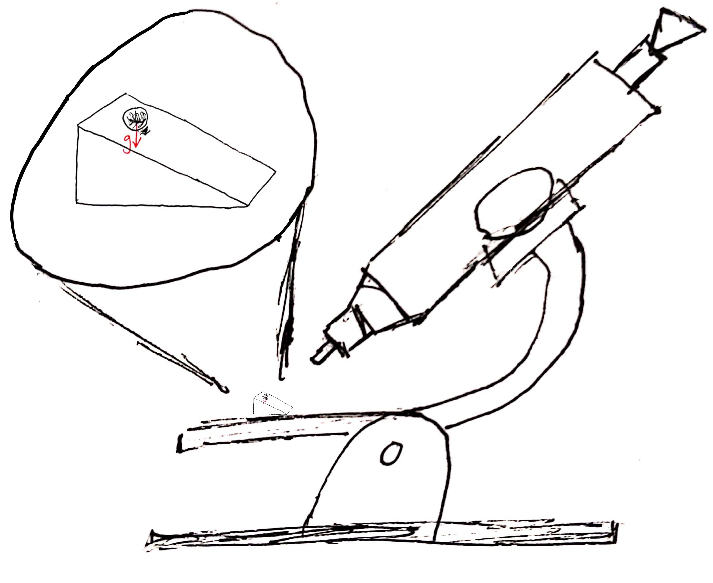
Figure 1: A cartoon of an experimental setup to look at miniature balls rolling down ramps, for which proper accounting of subleading effects may be necessary.

The construction of an appropriate effective description relies on three ingredients. The first is a list of the important degrees of freedom which specify the system under consideration—in particle physics this is often some fields $\left\{\phi_{i}\right\}$. The second is the set of symmetries which these degrees of freedom enjoy. These constrain the allowed interactions between our fields and so control the dynamics of the theory. Finally we need a notion of power counting, which organizes the effects in terms of importance. This will allow us to compute quantities to the desired precision systematically. Frequently in effective field theories of use in particle physics this role is played by $E/\Lambda$, where $E$ is an energy and $\Lambda$ is a heavy mass scale or cutoff above which we expect to require a new description of the physics.

1 Scale-dependence

We will often be interested in determining the appropriate description of a system at some scale, so it is necessary to understand which degrees of freedom and which interactions will be important as a function of energy. We can gain insight into when certain modes or couplings are important by studying the behavior of our system under scale transformations. Consider for example a theory of a real scalar field $\phi$, with action

$$S=\int\text{d}^{d}x\left(-\frac{1}{2}\partial_{\mu}\phi\partial^{\mu}\phi-\frac{1}{2}m^{2}\phi^{2}-\frac{1}{4!}\lambda\phi^{4}-\frac{1}{6!}\tau\phi^{6}+\dots\right),$$ (1)

where $d$ is the dimensionality of spacetime, $m,\lambda,\tau$ are couplings of interactions involving different numbers of $\phi$, the $\dots$ denote terms with higher powers of $\phi$, and we’ve imposed a $\mathbb{Z}_{2}:\phi\rightarrow-\phi$ symmetry for simplicity. We’ve set $c=\hbar=1$ leaving us with solely the mass dimension to speak of. From the fact that regardless of spacetime dimension we have $\left[S\right]=0$ and $\left[x\right]=-1$, where $\left[\cdot\right]$ denotes the mass dimension, we first calculate from the kinetic term that $\left[\phi\right]=\frac{d-2}{2}$, and then we can read off $\left[m^{2}\right]=2$, $\left[\lambda\right]=4-d$, $\left[\tau\right]=6-2d$. These are known as the classical dimension of the associated operators and are associated to the behavior of the operators at different energies, for the following reason.

If we wish to understand how the physics of this theory varies as a function of scale, we can perform a transformation $x^{\mu}\rightarrow sx^{\prime\mu}$ and study the long-distance limit $s\gg 1$ with $x^{\prime\mu}$ fixed. The measure transforms as $\text{d}^{d}x\rightarrow s^{d}\text{d}^{d}x^{\prime}$ and the derivatives $\partial_{\mu}\rightarrow s^{-1}\partial_{\mu^{\prime}}$. Then to restore canonical normalization of the kinetic term such that the one-particle states are properly normalized for the LSZ formula to work, we must perform a field redefinition $\phi(x)=s^{\frac{2-d}{2}}\phi^{\prime}(x^{\prime})$, and the action becomes

$$S=\int\text{d}^{d}x^{\prime}\left(-\frac{1}{2}\partial_{\mu^{\prime}}\phi^{\prime}\partial^{\mu^{\prime}}\phi^{\prime}-\frac{1}{2}m^{2}s^{2}\phi^{\prime 2}-\frac{1}{4!}\lambda s^{4-d}\phi^{\prime 4}-\frac{1}{6!}\tau s^{6-2d}\phi^{\prime 6}+\dots\right).$$ (2)

As a reminder, in the real world (at least at distances $\gtrsim 1\ \mu m$) we have $d=4$. As you look at the theory at longer distances the mass term becomes more important, so is known as a ‘relevant’ operator. One says that the operator $\phi^{2}$ has classical dimension $\Delta_{\phi^{2}}=2$. The quartic interaction is classically constant under such a transformation, so is known as ‘marginal’ with $\Delta_{\phi^{4}}=0$, and interactions with more powers of $\phi$ shrink at low energies and are termed ‘irrelevant’, e.g. $\Delta_{\phi^{6}}=-2$. We have been careful to specify that these are the classical dimension of the operators, also called the ‘engineering dimension’ or ‘canonical dimension’, which has a simple relation to the mass dimension as $\Delta_{\mathcal{O}}=d-\left[\mathcal{O}\right]$ for some operator $\mathcal{O}$. If the theory is not scale-invariant then quantum corrections modify this classical scaling by an ‘anomalous dimension’ $\delta_{\mathcal{O}}(m^{2},\lambda,\tau,\dots)$ which is a function of the couplings of the theory, and the full behavior is known as the ‘scaling dimension’. The terms ‘marginally (ir)relevant’ are used for operators whose classical dimension is zero but whose anomalous dimensions push them to one side.

The connection to the typical EFT power counting in $(E/\Lambda)$ is immediate. In an EFT with UV cutoff $\Lambda$, it’s natural to normalize all of our couplings with this scale and rename e.g. $\tau\rightarrow\bar{\tau}\Lambda^{6-2d}$ where $\bar{\tau}$ is now dimensionless. It’s easy to see that the long-distance limit is equivalently a low-energy limit by considering the derivatives, which pull down a constant $p^{\prime\mu}$ and scale as $s^{-1}$—or by simply invoking the uncertainty principle. Operators with negative scaling dimension contribute subleading effects at low energies precisely because of these extra powers of a large inverse mass scale.

2 Bottom-up or Top-down

Then he made the tank of cast metal, 10 cubits across from brim to brim, completely round; it was 5 cubits high, and it measured 30 cubits in circumference.

God on the merits of working to finite precision
1 Kings 7:23, Nevi’im
New Jewish Publication Society Translation (1985) [23]

The procedure of writing down the most general Lagrangian with the given degrees of freedom and respecting the given symmetries up to some degree of power counting is termed ‘bottom-up EFT’ as we’re constructing it entirely generally and will have to fix coefficients by making measurements. A great example is the Standard Model Effective Field Theory (SMEFT), of which the Standard Model itself is described by the SMEFT Lagrangian at zeroth order in the power counting. It is defined by being an $SU(3)\times SU(2)\times U(1)$ gauge theory with three generations of the following representations of left-handed Weyl fermions:

$3x$ Fermions	$SU(3)_{C}$	$SU(2)_{L}$	$U(1)_{Y}$
$Q$	3	2	$\frac{1}{6}$
$\bar{u}$	$\bar{3}$	-	$-\frac{2}{3}$
$\bar{d}$	$\bar{3}$	-	$\frac{1}{3}$
$L$	-	2	$-\frac{1}{2}$
$\bar{e}$	-	-	1

In addition the Standard Model contains one scalar, the Higgs boson, which is responsible for implementing the Anderson-Brout-Englert-Guralnik-Hagen-Higgs-Kibble-’t Hooft mechanism [24, 25, 26, 27, 28, 29] to break the electroweak symmetry $SU(2)_{L}\times U(1)_{Y}$ down to electromagnetism $U(1)_{Q}$ at low energies:

$H$	-	2	$-\frac{1}{2}$

The Standard Model Lagrangian contains all relevant and marginal gauge-invariant operators which can be built out of these fields, and has the following schematic form

$$\mathcal{L}_{\text{kin}} =-\frac{1}{4}F_{\mu\nu}F^{\mu\nu}-i\bar{\psi}\not{D}\psi-(D_{\mu}H)^{\dagger}(D^{\mu}H)$$ (3)

$$\mathcal{L}_{\text{Higgs}} =-yH\Psi\psi+\text{ h.c. }+m^{2}H^{\dagger}H-\frac{\lambda}{4}(H^{\dagger}H)^{2},$$ (4)

with $F$ a gauge field strength, $\psi$ a fermion, $D$ the gauge covariant derivative in the kinetic term Lagrangian on the first line, and the second line containing the Higgs’ Yukawa couplings and self-interactions. If a refresher on the Standard Model would be useful, the introduction to its structure toward the end of Srednicki’s textbook [18] will suffice for our purposes, while further discussion from a variety of perspectives can be found in Schwartz [22], Langacker [30], and Burgess & Moore [31].

The SMEFT power-counting is in energies divided by an as-yet-unknown UV scale $\Lambda$, so the dimension-$n$ SMEFT Lagrangian consists of all gauge-invariant combinations of these fields with scaling dimension $n-d$. At dimension five there is solely one operator, $\mathcal{L}^{(5)}=(LH)^{2}/\Lambda+\text{ h.c.}$, which contains a Majorana mass for neutrinos. In even-more-schematic form, the dimension six Lagrangian contains operators with the field content

$$-\Lambda^{2}\mathcal{L}^{(6)}=F^{3}+H^{6}+D^{2}H^{4}+\psi^{2}H^{3}+F^{2}H^{2}+\psi^{2}FH+\psi^{2}DH^{2}+\psi^{4},$$ (5)

where for aesthetics we have multiplied through by the scale $\Lambda$ and haven’t bothered writing down couplings. After understanding the structure of the independent symmetry-preserving operators (see e.g. [32, 33, 34]), the job of the bottom-up effective field theorist is to measure or constrain the coefficients of these higher-dimensional operators [35]. Useful data comes from both the energy frontier with searches at colliders for the production or decay of high-energy particles through these higher-dimensional operators and from the precision frontier measuring fundamental processes very well to look for deviations from the Standard Model predictions (e.g. [36, 37, 38]). For more detail, see the introduction to SMEFT by Brivio & Trott [39].

Another approach is possible when we already have a theory and just want to focus on some particular degrees of freedom. Then we may construct a ‘top-down EFT’ by taking our theory and ‘integrating out’ the degrees of freedom we don’t care about—for example by starting with the Standard Model above and getting rid of the electroweak bosons to focus on processes occurring at lower energies (e.g. Fermi’s model of the weak interaction [40]). We can’t necessarily just ignore those degrees of freedom though; what we need to do is modify the parameters of our EFT such that they reproduce the results of the full theory (to some finite precision) using only the low-energy degrees of freedom. Such a procedure can be illustrated formally by playing with path integrals. Consider the partition function for a theory with some light fields $\phi$ and some heavy fields $\Phi$:

$$Z=\int\mathcal{D}\phi\mathcal{D}\Phi\ e^{iS(\phi,\Phi)}.$$ (6)

This contains all of the physics in our theory, and so in principle we may use it to compute anything we wish. But if we’re interested in low-energy processes involving solely the $\phi$ fields, we could split up our path integral and first do the integral over the $\Phi$ fields. The light $\phi$ fields are the only ones left, so we can then write the partition function as

$$Z=\int\mathcal{D}\phi\ e^{iS_{\text{eff}}(\phi)},$$ (7)

where this defines $S_{\text{eff}}$. Thus far this still contains all the same physics, as long as we don’t want to know about processes with external heavy fields. But having decided that we are interested in the infrared physics of the $\phi$ fields, we can say that the effects of the heavy $\Phi$ fields will be suppressed by factors of the energies of interest divided by the mass of $\Phi$, and we should expand the Lagrangian $\mathcal{L}_{\text{eff}}$ in an appropriate series:

$$Z=\int\mathcal{D}\phi\ \text{exp}\left[i\int\text{d}^{d}x\left(\mathcal{L}_{0}(\phi)+\sum_{n=0}^{N}M_{\Phi}^{d-n}\sum_{i}\lambda_{i}^{(n)}\mathcal{O}_{i}^{(n)}(\phi)\right)\right],$$ (8)

where $\mathcal{L}_{0}(\phi)$ is the part of the full Lagrangian that had no heavy fields in it, $\mathcal{O}_{i}^{(n)}(\phi)$ is an operator of classical dimension $n$, $\lambda_{i}^{(n)}$ is a dimensionless coupling, and $N\geq d$ defines the precision to which one works in this effective theory. This is the procedure to find a top-down effective field theory in the abstract.

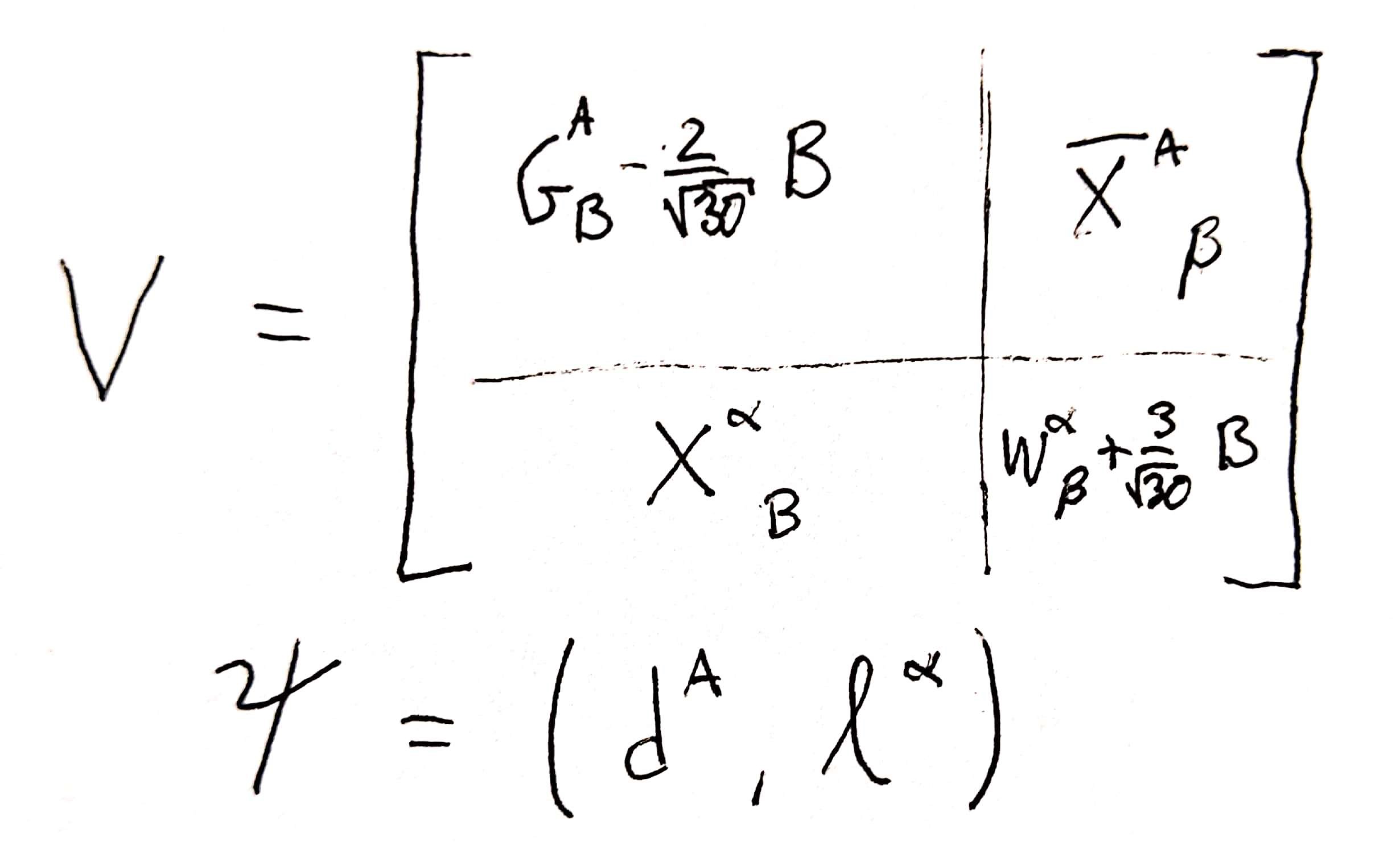
Figure 2: Schema of how the SM fits into $SU(5)$. The $SU(5)$ vector field $V$ decomposes into the gluons $G^{A}_{B}$, the $SU(2)_{L}$ vectors $W^{\alpha}_{\beta}$, hypercharge $B$ along the diagonal, and the new as-yet-unobserved leptoquarks $X^{\alpha}_{\beta}$ carrying both color and electroweak charge. The right-handed down-type quarks and the left-handed leptons are unified into an antifundamental. Decomposing the $10$ to find the rest of the SM fermions is left as an exercise.

A great example of a top-down EFT is in studying the Standard Model fields in the context of a Grand Unified Theory (GUT). Broadly, Grand Unification is the hope that there is some simpler, more symmetric theory behind the Standard Model which explains its structure. A GUT is a model in which the gauge groups of the SM are (partially [41]) unified in the UV. If there is a full unification to a single gauge factor, then this requires ‘gauge coupling unification’ in the UV until the symmetry is broken down to the SM gauge group at a high scale [42]. While one’s first exposure to this idea today may be in the context of a UV theory like string theory which roughly demands such unification, this was in fact first motivated by the observed infrared SM structure. It is frankly amazing that not only are the values of the SM gauge couplings consistent with this idea, and not only does $SU(3)\times SU(2)\times U(1)$ fit nicely inside $SU(5)$, but the SM fermion representations precisely fit into the $10\oplus\bar{5}$ representations of $SU(5)$ (see Figure 2). It’s hard to imagine a discovery that would have felt much more like one was obviously learning something deep and important about Nature than when Georgi realized how nicely all of this worked out. I’m reminded of Einstein’s words on an analogous situation in the early history of electromagnetism—the original unified theory:

The precise formulation of the time-space laws of those fields was the work of Maxwell. Imagine his feelings when the differential equations he had formulated proved to him that electromagnetic fields spread in the form of polarised waves, and with the speed of light! To few men in the world has such an experience been vouchsafed. At that thrilling moment he surely never guessed that the riddling nature of light, apparently so completely solved, would continue to baffle succeeding generations.
— Albert Einstein
Considerations concerning the Fundaments of Theoretical Physics, 1940 [43]

And just as with Maxwell, the initial deep insight into Nature was not the end of the story. As of yet, Grand Unification remains an unproven ideal, and indeed further empirical data has brought into question the simplest such schemes. But it’s hard to imagine all of this beautiful structure is simply coincidental, and I would wager that most high energy theorists still have a GUT in the back of their minds when they think about the UV structure of the universe, so this is an important story to understand. To learn generally about GUTs, I recommend the classic books by Kounnas, Masiero, Nanopoulos, & Olive [44] and Ross [45] or the recent book by Raby [46] for the more formally-minded. Shorter introductions can be found in Sher’s TASI lectures [47] or in the Particle Data Group’s Review of Particle Physics [48] from Hebecker & Hisano.

The structure of the simplest $SU(5)$ GUT is that the symmetry group breaks down to the SM at energies $M_{GUT}\sim 10^{16}\text{ GeV}$ via the Higgs mechanism. More generally, unification may proceed in stages as, for example, $SO(10)\rightarrow SU(4)_{c}\times SU(2)_{L}\times SU(2)_{R}\rightarrow SM$, and the breaking may occur via other mechanisms, as we’ll discuss further in Section 2. Back to our simple single-breaking example, as is familiar in the SM this means that the gauge bosons corresponding to broken generators get masses of order this GUT-breaking scale. As this is a far higher scale than we are currently able to directly probe, it is neither necessary nor particularly useful to keep these degrees of freedom fully in our description if we’re interesting in understanding the effects of GUT-scale fields. Rather than constructing the complete top-down EFT of the SM from a GUT, let’s focus on one particularly interesting effect.

One of the best ways to indirectly probe GUTs is by looking for proton decay. The GUT representations unify quarks and leptons, so the extra $SU(5)$ gauge bosons have nonzero baryon and lepton number and fall under the label of ‘leptoquarks’. It’s worth considering in detail why proton decay is a feature of GUTs and not of the SM, as it’s a subtler story than is usually discussed. While $U(1)_{B}$, the baryon number, is an accidental global symmetry of the SM, it’s an anomalous symmetry and so is not a symmetry of the quantum world. The ‘baryon minus lepton’ number, $U(1)_{B-L}$, is non-anomalous, but this is a good symmetry both of the SM and of a GUT and clearly does not prevent e.g. $p^{+}\rightarrow\pi^{0}e^{+}$. What’s really behind the stability of the proton is that, though $U(1)_{B}$ and $U(1)_{L}$ are not good quantum symmetries, the fact that they are good classical symmetries means their only violation is nonperturbatively by instantons. Such configurations yield solely baryon number violation by three units at once, corresponding to the number of generations, and thus the proton with $B=1$ is stable.

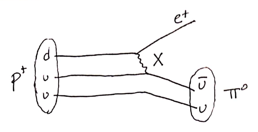
Figure 3: A representative diagram contributing to proton decay due to exchange of a heavy GUT gauge boson X.

But in GUTs, baryon number and lepton number are no longer accidental symmetries, so no such protection is available and the GUT gauge bosons mediate tree-level proton decay processes as in Figure 3. We can find the leading effect by integrating these out—in particular we’ll here look just at a four-fermion baryon-number-violating operator. The tree-level amplitude is simply

$$i\mathcal{M}(uude)=(ig)^{2}v_{u_{1}}\gamma^{\mu}u_{u_{2}}\frac{-i\left(\eta_{\mu\nu}+\frac{p^{\mu}p^{\nu}}{M_{GUT}^{2}}\right)}{p^{2}+M_{GUT}^{2}}v_{e}\gamma^{\nu}u_{d}\approx ig^{2}v_{u_{1}}\gamma^{\mu}u_{u_{2}}\frac{\eta_{\mu\nu}}{M_{GUT}^{2}}v_{e}\gamma^{\nu}u_{d}+\mathcal{O}(\frac{1}{M_{GUT}^{2}}),$$ (9)

so integrating out the gauge boson from this diagram gives us one of the contributions to the low-energy operators in Equation 8

$$\mathcal{O}=\frac{g^{2}}{2M_{\text{GUT}}^{2}}\epsilon_{\alpha\beta\gamma}\left(u_{R\alpha}\gamma_{\mu}u_{L\beta}\right)\left(e_{R}\gamma^{\mu}d_{L\gamma}\right),$$ (10)

where, in the notation of Equation 8, $\mathcal{O}_{i}^{(6)}=\epsilon_{\alpha\beta\gamma}\left(u_{R\alpha}\gamma_{\mu}u_{L\beta}\right)\left(e_{R}\gamma^{\mu}d_{L\gamma}\right),\lambda_{i}^{(6)}=g^{2}/2$ and $M_{\Phi}=M_{GUT}$. The calculation of the proton lifetime from this operator is quite complicated, but the dimensional analysis estimate of $\tau_{p}\sim M_{GUT}^{4}/g^{4}m_{p}^{5}$ actually works surprisingly well.

The job of the top-down effective field theorist is to calculate the effects of some particular UV physics on IR observables and by doing so understand how to search for their particular effects. While the effects will, by necessity, be some subset of the operators that the bottom-up effective field theorist has written down, the patterns and correlations present from a particular UV model can suggest or require particular search strategies. In the present context, a GUT may suggest the most promising final states to look for when searching for proton decay. If we wanted to calculate the lifetime and branching ratios more precisely we would have to deal with loop diagrams (among many complications), which of course is a generic feature. So we now turn our attention to the new aspects and challenges of field theory that appear once one goes beyond tree-level.

2 Renormalization

Renormalization is a notoriously challenging topic for beginning quantum field theorists to grok, and explanations often get bogged down in the details of one particular perspective or scheme or purpose and ‘miss the forest for the trees’, so to speak. We’ll attempt to overcome that issue by discussing a variety of uses for and interpretations of renormalization, as well as how they relate. And, of course, by examining copious examples and pointing out a variety of conceptual pitfalls.

Loops are necessary

At the outset the only fact one needs to have in mind is that renormalization is a procedure which lets quantum field theories make physical predictions given some physical measurements. Such a procedure was not necessary for a classical field theory, which is roughly equivalent to a quantum field theory at tree-level. A natural question for beginners to ask then is why we should bother with loops at all: Why don’t we just start off with the physical, measured values in the classical Lagrangian and be done with it? That is, if we measure, say, the mass and self-interaction of some scalar field $\phi$, let’s just define our theory

$$\mathcal{L}_{\text{exact}}\stackrel{{\scriptstyle?}}{{=}}-\frac{1}{2}\partial_{\mu}\phi\partial^{\mu}\phi-\frac{1}{2}m^{2}_{\text{phys}}\phi^{2}-\frac{1}{4!}\lambda_{\text{phys}}\phi^{4},$$ (11)

for some definitions of these physical parameters, and compute everything at tree-level. However, this does not constitute a sensible field theory, as the optical theorem tells us this is not consistent. We define $S=1+i\mathcal{M}$ as the S-matrix which encodes how states in the theory scatter, where the $1$ is the ‘trivial’ no-interaction part. Quantum mechanics turns the logical necessity that probabilities add up to 1 into the technical demand of ‘unitarity’, $S^{\dagger}S=1$, which tells us the nontrivial part must satisfy

$$i\left(\mathcal{M}^{\dagger}-\mathcal{M}\right)=\mathcal{M}^{\dagger}\mathcal{M}.$$ (12)

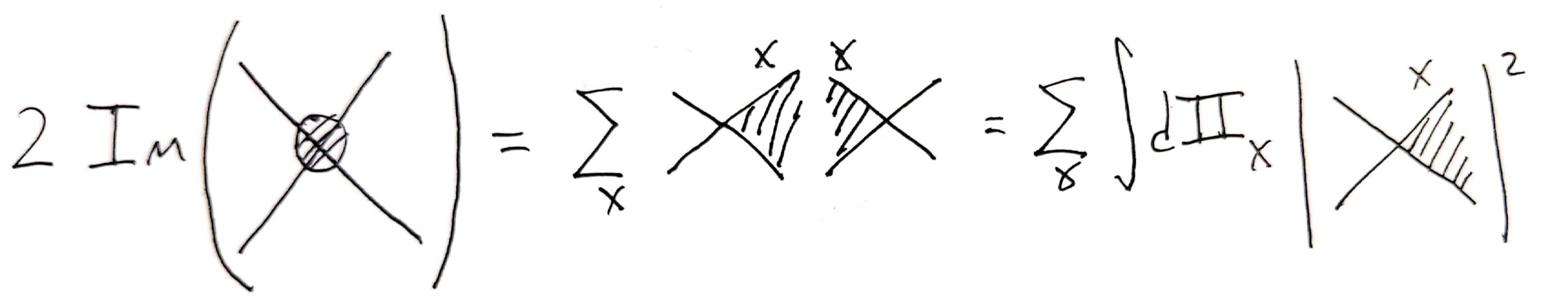
Figure 4: Schematic description of the optical theorem Equation 12 as applied to a $2\rightarrow 2$ process. On the right hand side one must sum over all possible intermediate states, including both various state labels $X$ and their phase space $\Pi_{X}$.

Sandwiching this operator equation between initial and final states, we find that the left hand side is the imaginary part of the amplitude $\mathcal{M}(i\rightarrow f)$, which is nonzero solely due to loops. This is depicted schematically in Figure 4. We can see why this is by examining a scalar field propagator. Taking the imaginary part one finds

$$\text{Im }\frac{1}{p^{2}+m^{2}+i\epsilon}=\frac{-\epsilon}{(p^{2}+m^{2})^{2}+\epsilon^{2}}.$$ (13)

This vanishes manifestly as $\epsilon\rightarrow 0$ except for when $p^{2}=-m^{2}$, and an integral to find the normalization yields

$$\text{Im }\frac{1}{p^{2}+m^{2}+i\epsilon}=-\pi\delta(p^{2}+m^{2}).$$ (14)

So internal propagators are real except for when the particle is put on-shell. In a tree-level diagram this occurs solely at some measure-zero set of exceptional external momenta, but in a loop-level diagram we integrate over all momenta in the loop, so an imaginary part is necessarily present. Now we see the necessity of loops solely from the conservation of probability and the framework of quantum mechanics.

The lesson to take away from this is that classical field theories produce correlation functions with some particular momentum dependence, which can be essentially read off from the Lagrangian. But a consistent theory requires momentum dependence of a sort that does not appear in such a Lagrangian, which demands that calculations must include loops. In particular it is the analyticity properties of these higher-order contributions that are required by unitarity, and there is an interesting program to understand the set of functions satisfying those properties at each loop order as a way to bootstrap the structure of multi-loop amplitudes (see e.g. [54, 55, 56, 57, 58, 59]).

So far from being ‘merely’ a way to deal with seemingly unphysical predictions, renormalization is very closely tied to the physics. We begin in the next section with understanding its use for removing divergences, as this is the most basic application and is often the first introduction students receive to renormalization. We will then move on to discuss other, more physical interpretations of renormalization.

1 To Remove Divergences

Physical input is required

As a first pass, let’s look again at a $\phi^{4}$ theory

$$\mathcal{L}=-\frac{1}{2}\partial_{\mu}\phi\partial^{\mu}\phi-\frac{1}{2}m_{0}^{2}\phi^{2}-\frac{1}{4!}\lambda_{0}\phi^{4},$$ (15)

and now treat it properly as a quantum field theory. As a simple example, let us consider $2\rightarrow 2$ scattering in this theory, our discussion of which is particularly influenced by Zee [20]. At lowest-order this is extremely simple, and the tree-level amplitude is $i\mathcal{M}(\phi\phi\rightarrow\phi\phi)=-i\lambda_{0}$. But if we’re interested in a more precise answer, we go to the next order in perturbation theory and we have the one-loop diagrams of Figure 5.

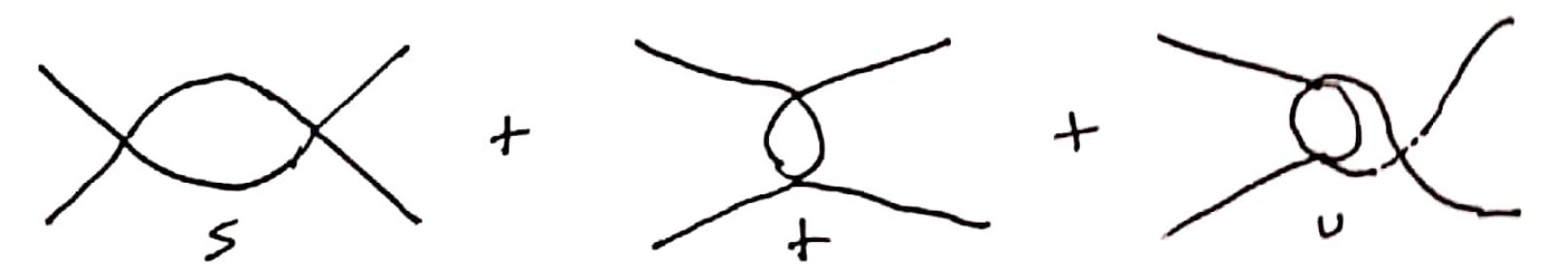
Figure 5: One-loop diagrams contributing to $2\rightarrow 2$ scattering in the $\phi^{4}$ theory. Since the external legs are all the same, these three different internal processes must be summed over, corresponding to momentum exchanged in the $s,t,u$ channels, where these are the Mandelstam variables [60].

Defining $P_{s}^{\mu}\equiv p_{1}^{\mu}+p_{2}^{\mu}$ as the momentum flowing through the loop in the $s$-channel diagram, that diagram is evaluated as

$$i\mathcal{M}(\phi\phi\rightarrow\phi\phi)_{\text{one-loop s-channel}}=(-i\lambda_{0})^{2}(-i)^{2}\frac{1}{2}\int\frac{d^{4}k}{(2\pi)^{4}}\frac{1}{P_{s}^{2}+m_{0}^{2}}\frac{1}{(P_{s}+k)^{2}+m_{0}^{2}}.$$ (16)

Just from power-counting, we can already see that this diagram will be divergent. In the infrared, as $k\rightarrow 0$, the diagram is regularized by the mass of the field, but in the ultraviolet $k\rightarrow\infty$, the integral behaves as $\sim\int d^{4}k/k^{4}\sim\int dk/k$ which is logarithmically divergent.

Though one might be tempted now to give up, we note that this divergence is appearing from an integral over very high energy modes—far larger than whatever energies we’ve verified our $\phi^{4}$ model to, so let’s try to ignore those modes and see if we can’t get a sensible answer. The general term for removing these divergences is ‘regularization’ and we will here regularize (or ‘regulate’) this diagram by imposing a hard momentum cutoff $\Lambda$ in Euclidean momentum space, which is the maximum energy of modes we let propagate in the loop. The loop amplitude may then be calculated with elementary methods detailed in, for example, Srednicki’s textbook [18]. First we introduce Feynman parameters to combine the denominators, using $(AB)^{-1}=\int_{0}^{1}dx(xA+(1-x)B)^{-2}$, which here tells us

$$\frac{1}{P_{s}^{2}+m_{0}^{2}}\frac{1}{(P_{s}+k)^{2}+m_{0}^{2}} =\int_{0}^{1}dx\left[x\left((P_{s}+k)^{2}+m_{0}^{2}\right)+(1-x)(P_{s}^{2}+m_{0}^{2})\right]^{-2}$$ (17)

$$=\int_{0}^{1}dx\left[q^{2}+D\right]^{-2},$$ (18)

where we’ve skipped the algebra letting us rewrite this with $q=k+xP_{s}$ and $D=x(1-x)P_{s}^{2}+m_{0}^{2}$. The change of variables $k\rightarrow q$ has trivial Jacobian, so the next step is to Wick rotate—Euclideanize the integral by defining $q^{0}=i\bar{q}^{d}$, such that $q^{2}\equiv q^{\mu}\eta_{\mu\nu}q^{\nu}=\bar{q}^{\mu}\delta_{\mu\nu}\bar{q}^{\nu}\equiv\bar{q}^{2}$. The measure simply picks up a factor of $i$, $d^{d}q=id^{d}\bar{q}$, and we can then go to polar coordinates via $d^{d}\bar{q}=\bar{q}^{d-1}d\bar{q}d\Omega_{d}$. Lorentz invariance then means the angular integral gives us the area of the unit sphere in $d$ dimensions, $\Omega_{d}=2\pi^{d/2}/\Gamma(d/2)$, where $\Omega_{4}=2\pi^{2}$, and the radial integral becomes

$$\int_{0}^{\Lambda}d\bar{q}\ \bar{q}^{3}\left[q^{2}+D\right]^{-2} =\left.\frac{1}{2}\left[\frac{D}{\bar{q}^{2}+D}+\log\left(\bar{q}^{2}+D\right)\right]\right|_{0}^{\Lambda}$$ (19)

$$=-\frac{1}{2}\left[\frac{\Lambda^{2}}{\Lambda^{2}+D}+\log\frac{D}{\Lambda^{2}+D}\right].$$ (20)

In fact it is possible to do the $x$ integral analytically here, but we’ll take $\Lambda^{2}\gg\left|P^{2}\right|\gg m^{2}$ to find a simple answer

$$-\frac{1}{2}\int_{0}^{1}dx\left[\frac{\Lambda^{2}}{\Lambda^{2}+D}+\log\frac{D}{\Lambda^{2}+D}\right]=\frac{1}{2}\left(1-\log\frac{P_{s}^{2}}{\Lambda^{2}}\right)+\dots$$ (21)

Now putting all that together and including all the diagrams up to one-loop, we get the form

$$\mathcal{M}(\phi\phi\rightarrow\phi\phi)=-\lambda_{0}+C\lambda_{0}^{2}\left[\log\left(\frac{\Lambda^{2}}{s}\right)+\log\left(\frac{\Lambda^{2}}{t}\right)+\log\left(\frac{\Lambda^{2}}{u}\right)\right]+\text{ subleading},$$ (22)

where $s,t,u$ are the Mandelstam variables and $C$ is just a numerical coefficient. Now we see explicitly that the divergence has led to dependence of our amplitude on our regulator $\Lambda$. Of course this is problematic because we introduced $\Lambda$ as a non-physical parameter, and it would not be good if our calculation of a physical low-energy observable depended sensitively on how we dealt with modes in the far UV. But let us try to connect this with an observable anyway. We note that the theory defined by the Lagrangian in Equation 15 can not yet be connected to an observable because we have not yet given a numerical value for $\lambda_{0}$. So let’s imagine an experimentalist friend of ours prepares some $\phi$s and measures this scattering amplitude at some particular angles and energies corresponding to values of the Mandelstam variables $s_{0},t_{0},u_{0}$. They find some value $\lambda_{\text{phys}}$, which is a pure number. If our theory is to describe this measurement accurately, this tells us a relation between our parameters and a physical quantity

$$-\lambda_{\text{phys}}=-\lambda_{0}+C\lambda_{0}^{2}\left[\log\left(\frac{\Lambda^{2}}{s_{0}}\right)+\log\left(\frac{\Lambda^{2}}{t_{0}}\right)+\log\left(\frac{\Lambda^{2}}{u_{0}}\right)\right]+\mathcal{O}(\lambda^{3}).$$ (23)

This is known as a ‘renormalization condition’ which tells us how to relate our quantum field theories to observations at non-trivial loop order. Since the left hand side is a physical quantity, it may worry us that the right hand side contains a non-physical parameter $\Lambda$. But we still haven’t said what $\lambda_{0}$ is, so perhaps we’ll be able to find a sensible answer if we choose $\lambda_{0}\equiv\lambda(\Lambda)$ in a correlated way with our regularization scheme. We call this ‘promoting $\lambda$ to a running coupling’ by changing from the ‘bare coupling’ $\lambda_{0}$ to one which depends on the cutoff. So let’s solve for $\lambda$ in terms of $\lambda_{\text{phys}}$ and $\Lambda$. Rearranging we have

$$\lambda_{0} =\lambda_{\text{phys}}+C\lambda_{0}^{2}\left[\log\left(\frac{\Lambda^{2}}{s_{0}}\right)+\log\left(\frac{\Lambda^{2}}{t_{0}}\right)+\log\left(\frac{\Lambda^{2}}{u_{0}}\right)\right]+\mathcal{O}(\lambda_{0}^{3})$$ (24)

$$\lambda(\Lambda) =\lambda_{\text{phys}}+C\lambda_{\text{phys}}^{2}\left[\log\left(\frac{\Lambda^{2}}{s_{0}}\right)+\log\left(\frac{\Lambda^{2}}{t_{0}}\right)+\log\left(\frac{\Lambda^{2}}{u_{0}}\right)\right]+\mathcal{O}(\lambda_{\text{phys}}^{3})$$ (25)

where in the second line the replacement $\lambda_{0}^{2}\mapsto\lambda_{\text{phys}}^{2}$ modifies the right side only at higher-order and so that is absorbed into our $\mathcal{O}(\lambda^{3})$ uncertainty. To see what this has done for us, let us plug this back into our one-loop amplitude Equation 22. This will impose our renormalization condition that our theory successfully reproduces our experimentalist friend’s result. We find

$$\mathcal{M}(\phi\phi\rightarrow\phi\phi)=-\lambda_{\text{phys}} -C\lambda_{\text{phys}}^{2}\left[\log\left(\frac{\Lambda^{2}}{s_{0}}\right)+\log\left(\frac{\Lambda^{2}}{t_{0}}\right)+\log\left(\frac{\Lambda^{2}}{u_{0}}\right)\right]$$ (26)

$$+C\lambda_{\text{phys}}^{2}\left[\log\left(\frac{\Lambda^{2}}{s}\right)+\log\left(\frac{\Lambda^{2}}{t}\right)+\log\left(\frac{\Lambda^{2}}{u}\right)\right]+\mathcal{O}(\lambda_{\text{phys}}^{3})$$

where again we liberally shunt higher-order corrections into our uncertainty term. Taking advantage of the nice properties of logarithms, we rearrange to get

$$\mathcal{M}(\phi\phi\rightarrow\phi\phi)=-\lambda_{\text{phys}}-C\lambda_{\text{phys}}^{2}\left[\log\left(\frac{s}{s_{0}}\right)+\log\left(\frac{t}{t_{0}}\right)+\log\left(\frac{u}{u_{0}}\right)\right]+\mathcal{O}(\lambda_{\text{phys}}^{3}).$$ (27)

We see that our renormalization procedure of relating our theory to a physical observable has enabled us to write the full amplitude in terms of physical quantities, and remove the divergence entirely. This one physical input at some particular kinematic configuration has enabled us to fully predict any $2\rightarrow 2$ scattering in this theory.

We thus see how the renormalization procedure removes the divergences in a naïve formulation of a field theory and allows us to make finite predictions for physical observables. While we did need to introduce a regulator, once we make the replacement $\lambda_{0}\rightarrow\lambda(\Lambda)$ as defined in Equation 25 (and similar replacements for the coefficients of the other operators), the one-loop divergences are gone. We are guaranteed that any one-loop correlation function we calculate is finite in the $\Lambda\rightarrow\infty$ limit, which removes the regulator. If we wanted to increase our precision and calculate now at two loops, we would first renormalize the theory at two loops analogously to the above, and would find a more precise definition for $\lambda(\Lambda)$ which included terms of order $\mathcal{O}(\lambda_{\text{phys}}^{3})$. At each loop order, replacing the bare couplings with running couplings suffices to entirely rid the theory of divergences.

Renormalizability

An important question is for which quantum field theories do a finite set of physical inputs allow the theory to be fully predictive, in analogy to the example above. Such a theory is called ‘renormalizable’ and means that after some finite number of experimental measurements, we can predict any other physics in terms of those values. Were this not the case, and no finite number of empirical measurements would fix the theory, it would not be of much use. Within the context of perturbation theory, a theory will be renormalizable if its Lagrangian contains solely relevant and marginal operators, and indeed for our $\phi^{4}$ theory three renormalization conditions are needed—one for each such operator.

The simplest way to understand why we must restrict to relevant and marginal operators is that irrelevant operators inevitably lead to the generation of a tower of more-and-more irrelevant operators. To see this, imagine now including a $\phi^{6}$ interaction, as depicted in Figure 6(a). At one loop this leads to a $4\rightarrow 4$ scattering process with the same sort of divergence we saw in our previous loop diagram. So this loop is probing the UV physics, but we cannot absorb the unphysical divergence into a local interaction in our Lagrangian unless we now include a $\phi^{8}$ term. But then we can draw a similar one-loop diagram with the $\phi^{8}$ interaction which will require a $\phi^{10}$ interaction, and so on. Note that in our $\phi^{4}$ theory we also have $4\rightarrow 4$ scattering at one loop, seen in Figure 6(b), but there it comes from a box diagram which is finite, and so there is no need to include more local operators.

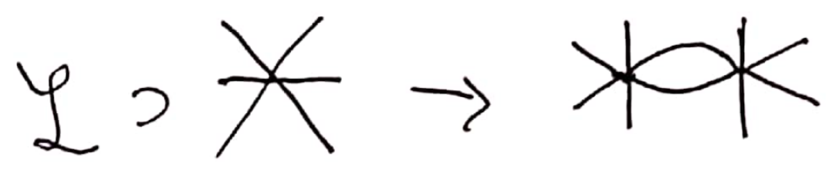
(a)

(b)

Figure 6: In (a), a pictoral representation of the nonrenormalizability of theories described by Lagrangians with irrelevant operators. A tree-level six-point coupling leads to a new divergence in $4\rightarrow 4$ scattering, which must be absorbed into a renormalized eight-point coupling, which would then beget a divergent $6\rightarrow 6$ amplitude …. Note that this does not mean there are not one-loop contributions to $4\rightarrow 4$ scattering. Such a diagram is depicted in (b), but it is finite and does not require additional local operators.

However, we emphasized above that the most useful description of a system depends on the precision at which one wishes to measure properties of the system. Thus in the study of effective field theories a broader definition of renormalizability should be used. For a theory with cutoff $\Lambda$, one decides to work to precision $\mathcal{O}(E/\Lambda)^{n}$ where $E$ is a typical energy scale of a process and $n$ is some integer. There are then a finite number of operators which contribute to processes to that precision—only those up to scaling dimension $n$—and so there is a notion of ‘effective renormalizability’ of the theory. We still require solely a finite number of inputs to set the behavior of the theory to whatever precision we wish, but such a theory nevertheless fails the original criterion, which may be termed ‘power counting renormalizability’ in comparison.

Wilsonian renormalization of $\phi^{4}$

Above we characterized our cutoff as an unphysical parametrization of physics at high scales that we do not know and we found that its precise value dropped out of our physically observable amplitude. To some extent this is rather surprising, as it’s telling us that the high energy modes in our theory have little effect on physics at long distances—we can compensate for their effects by a small shift in a coupling. We can gain insight into the effects of these high energy modes by taking the cutoff seriously and looking at what happens when the cutoff is lowered. This brilliant approach due to Wilson [61] is aimed at providing insight as to the particular effects of these high-energy modes by integrating out ‘shells’ of high-energy Euclidean momenta and looking at the low-energy effects. This discussion is closely inspired by that in Peskin & Schroeder’s chapter 12 [19], as well as Srednicki’s chapter 29 [18].

It is easiest to see how to implement this by considering the path integral formulation. We can equally well integrate over position space paths as over momentum modes:

$$Z=\int\mathcal{D}\phi(x)e^{i\int\mathcal{L}(\phi)}=\left({\displaystyle\prod_{k}}\int\text{d}\phi(k)\right)e^{i\int\mathcal{L}(\phi)},$$ (28)

and here it is clear that we may integrate over particular momentum modes separately if we so choose. In the condensed matter application in which Wilson originally worked, a cutoff appears naturally due to the lattice spacing $a$ giving an upper bound on momenta $k_{\text{max}}\sim 1/a$. In a general application we can imagine defining the theory with a fundamental cutoff $\Lambda$ by including in the path integral only modes with Euclidean momentum $k^{2}\leq\Lambda^{2}$. The theory is defined by the values of the parameters in the theory with that cutoff—our familiar relevant and marginal operators $m^{2}(\Lambda),\lambda(\Lambda)$ and in principle all of the ‘Wilson coefficients’ of irrelevant operators as well, since the theory is manifestly finite. The idea is to effectively lower the cutoff by explicitly integrating out modes with $b\Lambda\leq k\leq\Lambda$ for some $b<1$. This will leave us with a path integral over modes with $k^{2}\leq b^{2}\Lambda^{2}$—which is a theory of the same fields now with a cutoff $b\Lambda$. By integrating out the high-energy modes we’ll be able to track precisely their effects in this low-energy theory.

Peskin & Schroeder perform this path integral explicitly by splitting the high energy modes into a different field variable and quantizing it, but since we’ve already introduced the conceptual picture of integrating fields out we’ll take the less-involved approach of Srednicki. To repeat what we discussed above, the diagrammatic idea of integrating out a field is to remove it from the spectrum of the theory and reproduce its effects on low-energy physics by modifying the interactions of the light fields. Performing the path integral over some fields does not change the partition function, so the physics of the other fields must stay the same. We want to do the same thing here, but integrate out solely the high energy modes of a field and reproduce the physics in terms of the light modes.

We’ll continue playing around with $\phi^{4}$ theory and define our (finite!) theory with a cutoff of $\Lambda$, which in full generality looks like:

$$\mathcal{L}(\Lambda)=-\frac{1}{2}Z(\Lambda)\partial_{\mu}\phi\partial^{\mu}\phi-\frac{1}{2}m^{2}(\Lambda)\phi^{2}-\frac{1}{4!}\lambda(\Lambda)\phi^{4}-\sum\limits_{n=3}^{\infty}\frac{c_{n}(\Lambda)}{(2n)!}\phi^{2n}.$$ (29)

For simplicity we will decree that at our fundamental scale $\Lambda$ we have a canonically normalized field $Z(\Lambda)=1$ and no irrelevant interactions $c_{n}(\Lambda)=0$, but just some particular $m^{2}(\Lambda)$ and $\lambda(\Lambda)$.

Let’s look first at the one-loop four-point amplitude, which we must ensure is the same in both the theory with cutoff $\Lambda$ and that with cutoff $b\Lambda$. In the original theory, the amplitude at zero external momentum is

$$iV_{4}^{\Lambda}(0,0,0,0)=-i\lambda(\Lambda)+\frac{3}{2}(-i\lambda(\Lambda))^{2}\int_{|k|<\Lambda}\frac{d^{4}k}{(2\pi)^{4}}\frac{(-i)^{2}}{(k^{2}+m^{2}(\Lambda))^{2}}+\mathcal{O}(\lambda^{3})$$ (30)

When we evaluate this in the theory with a lowered cutoff $b\Lambda$, the modification is simply to everywhere make the replacement $\Lambda\mapsto b\Lambda$. In order for the physics to remain the same without the high-energy modes, the vertex function must not change. We’ll take full advantage of the perturbativity of the result—that is, $\lambda(\Lambda)-\lambda(b\Lambda)\sim\mathcal{O}(\lambda^{2})$, $m^{2}(\Lambda)-m^{2}(b\Lambda)\sim\mathcal{O}(\lambda^{2})$—to swap out quantities evaluated at $b\Lambda$ in the second-order term for those evaluated at $\Lambda$ at the cost solely of higher-order terms which we ignore.

$$0 \equiv V_{4}^{\Lambda}(0,0,0,0)-V_{4}^{b\Lambda}(0,0,0,0)$$ (31)

$$=-\lambda(\Lambda)+\frac{3}{2}\lambda(\Lambda)^{2}\int_{|\bar{k}|<\Lambda}\frac{d^{4}\bar{k}}{(2\pi)^{4}}\frac{1}{(\bar{k}^{2}+m^{2}(\Lambda))^{2}}$$

$$+\lambda(b\Lambda)-\frac{3}{2}\lambda(b\Lambda)^{2}\int_{|\bar{k}|<b\Lambda}\frac{d^{4}\bar{k}}{(2\pi)^{4}}\frac{1}{(\bar{k}^{2}+m^{2}(b\Lambda))^{2}}$$

$$=-\lambda(\Lambda)+\lambda(b\Lambda)+\frac{3}{2}\lambda(\Lambda)^{2}\int_{|\bar{k}|=b\Lambda}^{\Lambda}\frac{d^{4}\bar{k}}{(2\pi)^{4}}\frac{1}{(\bar{k}^{2}+m^{2}(\Lambda))^{2}}+\mathcal{O}(\lambda^{3})$$

$$=-\lambda(\Lambda)+\lambda(b\Lambda)+\frac{3}{16\pi^{2}}\lambda(\Lambda)^{2}\log\left(\frac{\Lambda}{b\Lambda}\right)+\mathcal{O}(\lambda^{3},\frac{m^{2}}{\Lambda^{2}})$$

$$\Rightarrow\lambda(b\Lambda) =\lambda(\Lambda)-\frac{3}{16\pi^{2}}\lambda(\Lambda)^{2}\log\left(\frac{1}{b}\right)+\dots$$ (32)

The effect of high energy modes on the four-point vertex function can be simply absorbed into a shift in the coupling constant! This procedure explicitly transfers loop-level physics in the theory defined at $\Lambda$ into tree-level physics at $b\Lambda$.

We can repeat this for the two point function to find the behavior of $Z(\Lambda)$ and $m^{2}(\Lambda)$.

$$0 \equiv\Sigma^{\Lambda}(p)-\Sigma^{b\Lambda}(p)$$ (33)

$$=Z(\Lambda)p^{2}+m^{2}(\Lambda)+\lambda(\Lambda)\int_{|\bar{k}|<\Lambda}\frac{d^{4}\bar{k}}{(2\pi)^{4}}\frac{1}{(Z(\Lambda)\bar{k}^{2}+m^{2}(\Lambda))}$$

$$-Z(b\Lambda)p^{2}-m^{2}(b\Lambda)-\lambda(b\Lambda)\int_{|\bar{k}|<b\Lambda}\frac{d^{4}\bar{k}}{(2\pi)^{4}}\frac{1}{(Z(b\Lambda)\bar{k}^{2}+m^{2}(b\Lambda))}$$

$$=\left[Z(\Lambda)-Z(b\Lambda)\right]p^{2}+m^{2}(\Lambda)-m^{2}(b\Lambda)+\lambda(\Lambda)\int_{|\bar{k}|=b\Lambda}^{\Lambda}\frac{d^{4}\bar{k}}{(2\pi)^{4}}\frac{1}{(Z(\Lambda)\bar{k}^{2}+m^{2}(\Lambda))}$$

$$=\left[Z(\Lambda)-Z(b\Lambda)\right]p^{2}+\left[m^{2}(\Lambda)-m^{2}(b\Lambda)\right]+\frac{\lambda(\Lambda)}{16\pi^{2}}\left[\Lambda^{2}-b^{2}\Lambda^{2}\right]+\lambda(\Lambda)\frac{m^{2}(\Lambda)}{8\pi^{2}}\log\left(\frac{1}{b}\right)$$

$$\Rightarrow Z(b\Lambda) =Z(\Lambda)+\mathcal{O}(\lambda^{2})$$ (34)

$$\Rightarrow m^{2}(b\Lambda) =m^{2}(\Lambda)+\frac{\lambda(\Lambda)}{16\pi^{2}}\Lambda^{2}\left[1-b^{2}\right]-\lambda(\Lambda)\frac{m^{2}(\Lambda)}{8\pi^{2}}\log\left(\frac{1}{b}\right)+\dots$$ (35)

We have again liberally ignored subleading terms. We see that the wavefunction normalization $Z$ does not run at one-loop in this theory, since the only one-loop diagram contributing to the two-point function does not have external momentum routed through the loop. This is merely ‘accidental’ as $Z$ is not symmetry-protected and does run at two-loops. We also see the first hints of a somewhat worrisome situation with scalar masses. The mass $m^{2}(\Lambda)$ receives large one-loop corrections which tend to raise the mass up to near the cutoff, regardless of whether we originally had $m^{2}(\Lambda)\ll\Lambda^{2}$. We will investigate this in great detail later.

Now imagine we want to measure some properties of $\phi$ particles with external momenta far below our fundamental cutoff $p_{i}\sim\mu\ll\Lambda$. By construction, our procedure of integrating out high-energy momentum modes keeps the physics of these low-energy particles the same. But if we calculate this scattering amplitude using $\mathcal{L}(\Lambda)$, it is not easy to see from the Lagrangian how these low-energy modes will behave, since important effects are hidden in loop diagrams. If we instead first integrate out momentum shells down to some $\mathcal{L}(b\Lambda)$ with $\mu<b\Lambda\ll\Lambda$, then the effects of the high energy modes have been absorbed into the parameters of our Lagrangian, and we can read off much more of how $\phi$ particles will behave at low energies simply by looking at the parameters.

We can see further value in this approach if we consider scattering more low-energy $\phi$. Let’s look at the $6$-point vertex function at zero momentum—in the theory at $\Lambda$, we start with $c_{6}(\Lambda)=0$ and a one-loop diagram where momenta up to $\Lambda$ run in the loop:

$$V_{6}^{\Lambda}=\frac{\lambda^{3}(\Lambda)}{48}\int_{|k|<\Lambda}\frac{d^{4}k}{(2\pi)^{4}}\left(\frac{1}{Z(\Lambda)k^{2}+m^{2}(\Lambda)}\right)^{3}.$$ (36)

Now in the theory at $b\Lambda$, the loop only contains momenta up to $b\Lambda$, so we must account for the difference with a contact interaction $c_{6}(b\Lambda)$:

$$V_{6}^{b\Lambda}=c_{6}(b\Lambda)+\frac{\lambda^{3}(b\Lambda)}{48}\int_{|k|<b\Lambda}\frac{d^{4}k}{(2\pi)^{4}}\left(\frac{1}{Z(b\Lambda)k^{2}+m^{2}(b\Lambda)}\right)^{3}.$$ (37)

Again we should ensure that the physics is the same upon lowering the cutoff:

$$0 \equiv V_{6}^{\Lambda}-V_{6}^{b\Lambda}$$ (38)

$$c_{6}(b\Lambda) =\frac{\lambda^{3}(\Lambda)}{48}\int_{b\Lambda}^{\Lambda}\frac{d^{4}k}{(2\pi)^{4}}\left(\frac{1}{Z(\Lambda)k^{2}+m^{2}(\Lambda)}\right)^{3}$$ (39)

$$=\frac{\lambda(\Lambda)^{3}}{3\times 256\pi^{2}}\left(\frac{1}{(b\Lambda)^{2}}-\frac{1}{\Lambda^{2}}\right)+\dots$$ (40)

So this renormalization procedure is especially useful for understanding the behavior of irrelevant interactions. In our original theory nothing about the six-particle interaction was obvious from the Lagrangian, but in our theory with cutoff $b\Lambda$ we can simply read off the strength of this interaction at lowest order.

Note also the inverse behavior to that of the mass corrections—for the irrelevant interaction, the most significant contributions to the infrared behavior come from the low-energy part of the loop integral, and the UV contributions are suppressed relative to this. Similarly, if we had started with a nonzero $c_{6}(\Lambda)$ which was small in units of the cutoff $c_{6}(\Lambda)\ll\Lambda^{-2}$ (so perturbative), such a UV contribution will also be subdominant. Then fully generally here, we have

$$c_{6}(b\Lambda)\simeq\frac{\lambda(\Lambda)^{3}}{16\pi^{2}}\frac{1}{b^{2}\Lambda^{2}}+\mathcal{O}(b^{0})$$ (41)

as we evolve to low scales $b\ll 1$.

The Wilsonian approach we have discussed here gives useful intuition for how renormalization works as a coarse-graining procedure wherein one changes the fundamental ‘resolution’ of the theory, but in practice can make calculations cumbersome. Furthermore, the hard momentum-space cutoff we used is not gauge-invariant, which causes difficulties in realistic applications.

The benefit, however, is that this is a ‘physical renormalization scheme’ in which the renormalization condition relates the bare parameters to physical observables. For this reason, this renormalization scheme satisfies the Appelquist-Carrazone decoupling theorem [62], which is enormously powerful. This guarantees for us that the effects of massive fields can, at low energies, simply be absorbed into modifications of the parameters in an effective theory containing solely light fields.

In the next section we’ll return to a clarifying example of the meaning of the decoupling theorem, and also discuss a renormalization scheme which does not satisfy the requirements for this theorem to operate, but is far simpler to use for calculations. The winning strategy will be to input decoupling by hand, which will allow us to get sensible physical results without the computational difficulty. Before we get to that, though, we’ll take a couple detours.

Renormalization and locality

We have seen that the need to remove divergences in our theory led to the introduction of running couplings which change as a function of scale. In our example above we see that renormalization has the operational effect of transferring loop-level physics into the tree-level parameters. This is an interesting perspective which bears further exploration—if there is hidden loop-level physics that really has the same physical effects as the tree-level bare parameters, perhaps this is a sign that there is a better way to organize our perturbation theory. Indeed, at some very general level renormalization can be thought of as a method for improving the quality of perturbation theory. For useful discussions at this level of abstraction of how renormalization operates, see [63] for its natural appearance whenever infinities are encountered in naïve perturbative calculations, and [64] for its usefulness even when infinities are not present. We’ll discuss this perspective on renormalization further in the next section.

However it’s clear that loops also give rise to physics that is starkly different from the lowest-order result (e.g. non-trivial analytic structure), so how do we know what higher-order physics we can stuff into tree-level? In a continuum quantum field theory, a Lagrangian is a local object $\mathcal{L}(x)$—that is, it contains operators like $\phi(x)^{3}$ which give an interaction between three $\phi$ modes at a single spacetime point $x$. Such effects are known as ‘contact interactions’, but even at tree-level a local Lagrangian can clearly produce non-local (that is, long-range) physics effects. For example, consider the amplitude for $2\rightarrow 2$ scattering in a $\phi^{3}$ theory at second order in the coupling.

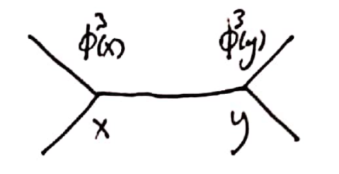
Figure 7: A position space Feynman diagram with vertices labeled.

In position space the non-locality here is obvious, as in Figure 7: A simple tree-level diagram corresponds to a particle at point $x$ and a particle at point $y$ exchanging a $\phi$ quantum, but one may forget this important fact when working in momentum space. There the result is

$$i\mathcal{M}(\phi\phi\rightarrow\phi\phi)=\frac{ig^{2}}{p^{2}+m^{2}},$$ (42)

and indeed, Fourier transforming the cross-section for this process yields a Yukawa scattering potential for our $\phi$ particles, showing that they mediate a long-range force over distances $r\sim 1/m$. We obviously cannot redefine the Lagrangian to put this effect into the lowest order of perturbation theory since this is not a local effect.

But if we do have a continuum quantum field theory, then because of locality it describes fluctuations on all scales. When we go to loop-level, we must integrate over all possible internal states, which includes integrating over arbitrarily large momenta or equivalently fluctuations on arbitrarily small scales. Heuristically, when the loop integral is sensitive to the ultraviolet of the theory, it is computing effects that operate on all scales—that is, it gives a contribution to local physics. This tells us that the pieces of this higher-order contribution which we can reshuffle into our Lagrangian are connected with ultraviolet sensitivity, leading to a close connection of renormalization with divergences.

A couple notes are warranted about the notion of locality we rely on here. Firstly, it’s clear that this criterion of local effects appears because we began with a local Lagrangian. If we postulated that our fundamental theory contained nonlocal interactions, say $\mathcal{L}(x)\supset g\phi(x)\left(\int dy\phi(y)\right)\left(\int dz\phi(z)\right)$, then we could clearly absorb further nonlocalities with the same structure into this coupling as well. However, this sort of nonlocality is different from the nonlocality we saw appearing out of the local theory at tree-level. In particular it would break the standard connection between locality and the analytic structure of amplitudes—see e.g. Schwartz [22] or Weinberg [65] on ‘polology’ and locality.

Secondly, our notion of locality should be modified in a low-energy theory with an energy-momentum cutoff $\Lambda$, as can be seen in hindsight in our Wilsonian discussion above. As $\Lambda$ defines a maximum energy scale we can probe, there is equivalently a minimum time and length scale we can probe due to the uncertainty principle, heuristically $\Delta x^{\mu}\gtrsim 1/\Delta p^{\mu}\gtrsim 1/\Lambda$. As a result, any fluctuations on shorter length scales are effectively local from the perspective of the low-energy theory. An exchange of a massive field with $M>\Lambda$ or of a light field with high frequency $\omega>\Lambda$ appears instantaneous to low-energy observers. This explains how it’s sensible to use renormalization techniques in, for example, condensed matter applications, where systems are fundamentally discrete.

We can see this concretely by imagining the light $\phi$s in the tree-level example above instead exchanged a heavier scalar $\Phi$ with mass $M\gg m$. While the amplitude $\mathcal{M}=g^{2}/(p^{2}+M^{2})$ is still nonlocal in the continuum theory, if we’re only interested in physics at energies $E\ll M$ we may Taylor expand the result $\mathcal{M}=g^{2}/M^{2}+g^{2}p^{2}/2M^{4}+\dots$. We may then absorb the leading effects of this heavy scalar into an effectively local interaction $g^{2}\phi^{4}/M^{2}$ among the light fields—as long as we work at energies below $M$.

In the next section we’ll explore concretely how these insights enable us to transfer loop-level physics to tree-level physics, and so improve our calculations.

2 To Repair Perturbation Theory

Renormalization group equations

The astute reader may notice a potential issue with our one-loop results in the $\phi^{4}$ theory, Equations 32,34,35. We’ve derived this behavior as the first subleading terms in a series expansion in the number of loops. In relation to the tree-level results, the one-loop contributions are suppressed by a factor $\sim\lambda/16\pi^{2}\log(\Lambda_{0}/\Lambda)$, where I’ve switched notation to now have $\Lambda_{0}$ as a high scale and $\Lambda$ as the lower scale we integrate down to. Higher $n$-loop contributions will be further suppressed by $n$ loop factors. But what if we wanted to study physics at a scale far lower than $\Lambda_{0}$? Eventually this factor becomes large enough that we will need to compute many loops to obtain high precision, and then large enough that we have reason to question the convergence of the series. Keep in mind that we are in the era of precision measurements of the Standard Model, so these one-loop expressions are very restrictive.

For a concrete example, say we wanted to check the SM prediction for a measurement of a coupling $\lambda(\Lambda)$ with $\lambda(\Lambda_{0})=1$ whose experimental uncertainty was $1\%$. Let’s define a theoretical uncertainty on a perturbative calculation to $n^{\text{th}}$ order as

$$\epsilon_{n}\equiv\frac{n^{\text{th}}\text{ order result}-\text{ estimated size of }(n+1)^{\text{th}}\text{ order result}}{n^{\text{th}}\text{ order result}},$$ (43)

where our Wilsonian calculation in Section 1 gave at first order, as a reminder (and with modified notation)

$$\lambda(\Lambda)=\lambda(\Lambda_{0})-\frac{3}{16\pi^{2}}\lambda(\Lambda_{0})^{2}\log\frac{\Lambda_{0}}{\Lambda}+\mathcal{O}(\lambda^{3}),$$ (44)

and our heuristic estimate for the size of the second order correction is $(\frac{3}{16\pi^{2}})^{2}\lambda(\Lambda_{0})^{3}\log^{2}\frac{\Lambda_{0}}{\Lambda}$. When the result is simply a series, the uncertainty is very simple to calculate, as the numerator is then our estimate of the $(n+1)^{\text{th}}$ order correction, which is roughly the square of the first order correction in this case for $n=1$. Here we have $\epsilon_{1}=\frac{3}{16\pi^{2}}\lambda(\Lambda_{0})\log\frac{\Lambda_{0}}{\Lambda}$.

Then in order for our theoretical uncertainty to be subdominant to the experimental precision, $\epsilon_{1}<0.01$, we must go past the one-loop result if we wish to look at energies below $\Lambda\sim\exp(-16\pi^{2}\times 0.01/3)\Lambda_{0}\sim\Lambda_{0}/2$, the two-loop result is only sufficient until $\Lambda\sim\Lambda_{0}/400$, and if we can manage to calculate the three-loop corrections that only gets us down to something like $\Lambda\sim\Lambda_{0}/8\times 10^{4}$. If we’re interested in taking the predictions of a Grand Unified Theory defined at $\Lambda_{0}\sim 10^{16}\text{ GeV}$ and comparing them to predictions at SM energies, how in the world are we to do so?

Fortunately, we can do better by applying our one-loop results more cleverly. It is clear by looking at Equations 32,34,35 that the results have the same form no matter the values of $\Lambda_{0},\Lambda$. So if we take $\Lambda$ to be only slightly smaller than $\Lambda_{0}$ (corresponding to $1-b\ll 1$ in our previous notation) the expansion parameter becomes very small and the one-loop result becomes very trustworthy. What we would like is some sort of iterative procedure to gradually lower the cutoff, which we could then use to find the one-loop result for energies far lower than the range of our perturbative series. This is in fact precisely the sort of problem that a differential equation solves, and we can derive such an equation by differentiating both sides by $\ln\Lambda$ and then taking $\Lambda$ infinitesimally close to $\Lambda_{0}$. That exercise yields

$$\frac{\text{d}Z(\Lambda)}{\text{d}\log\Lambda} =0$$ (45)

$$\frac{\text{d}m^{2}(\Lambda)}{\text{d}\log\Lambda} =\frac{\lambda(\Lambda)}{8\pi^{2}}\left(m^{2}(\Lambda)-\Lambda^{2}\right)$$ (46)

$$\frac{\text{d}\lambda(\Lambda)}{\text{d}\log\Lambda} =\frac{3}{16\pi^{2}}\lambda(\Lambda)^{2}$$ (47)

These are known as ‘renormalization group equations’ and they indeed allow us to evolve the coupling down to low energies—one says we use them to ‘resum the logarithm’. Then to study physics at a very low scale we can bring these couplings down to a lower scale and do our loop expansion using those couplings, which is known as ‘renormalization group improved perturbation theory’, and which we will discuss in more detail soon. Explicitly solving with our boundary condition at $\Lambda_{0}$ yields

$$\lambda(\Lambda)=\frac{\lambda(\Lambda_{0})}{1+\frac{3\lambda(\Lambda_{0})}{16\pi^{2}}\log\frac{\Lambda_{0}}{\Lambda}}$$ (48)

Turning back to our effective field theory language, we see that quantum corrections have generated an anomalous dimension for $\lambda$, $\delta_{\phi^{4}}=3\lambda^{2}/(16\pi^{2})$, correcting the leading order scaling behavior. Since $\delta_{\phi^{4}}>0$, we’ve determined that the quartic interaction is marginally irrelevant, which we will return to later.

We can now look at the theoretical uncertainty in this one-loop resummed calculation by including an estimate of the next order correction to the running of the quartic $\frac{\text{d}\lambda(\Lambda)}{\text{d}\log\Lambda}=\frac{3}{16\pi^{2}}\lambda(\Lambda)^{2}+\left(\frac{3}{16\pi^{2}}\right)^{2}\lambda(\Lambda)^{3}$ and resumming that expression. This can no longer be done analytically, but numerical evaluation easily reveals that the theoretical uncertainty here stays below $1\%$ for many, many orders of magnitude below $\Lambda_{0}$. Resumming the logarithmic corrections allows us to use our loop results to far greater effect.

Decoupling

The physical meaning and technical statement of the decoupling theorem commonly confuse even prominent practitioners of effective field theory, so it’s worth going clearly through an example to refine our understanding. Indeed, one may be confused just at zeroth order about how decoupling is sensible against the background of the hierarchy problem—which is an issue of sensitivity of a scalar mass to heavy mass scales. How can we claim QFT obeys a decoupling theorem and then go on to worry at length about quantum corrections $\delta m^{2}\propto M^{2}$?

The correct way to think about the decoupling theorem is not whether a top-down calculation could yield a result that depends on heavy mass scales, but whether a bottom-up effective field theorist and low-energy observer could gain information about the heavy mass scales through low-energy measurements. We can clarify this important difference by looking at a one-loop mass correction to a light scalar $\phi$ of mass $m$ from a heavy scalar $\Phi$ of mass $M$ through the interaction $\lambda\phi^{2}\Phi^{2}$. We again take a Wilsonian perspective and begin at a scale $\Lambda_{0}>M$. In close analogy to what we had before, we now find

$$0 \equiv\Sigma^{\Lambda_{0}}(0)-\Sigma^{\Lambda}(0)$$ (49)

$$=m^{2}(\Lambda_{0})+\lambda(\Lambda_{0})\int_{|k|<\Lambda_{0}}\frac{d^{4}k}{(2\pi)^{4}}\frac{1}{(k^{2}+M^{2}(\Lambda_{0}))}$$

$$-m^{2}(\Lambda)-\lambda(\Lambda)\int_{|k|<\Lambda}\frac{d^{4}k}{(2\pi)^{4}}\frac{1}{(k^{2}+M^{2}(\Lambda))}$$

$$=m^{2}(\Lambda_{0})-m^{2}(\Lambda)+\lambda(\Lambda_{0})\int_{|k|=\Lambda}^{\Lambda_{0}}\frac{d^{4}k}{(2\pi)^{4}}\frac{1}{(k^{2}+M^{2}(\Lambda_{0}))}$$

$$=\left[m^{2}(\Lambda_{0})-m^{2}(\Lambda)\right]+\frac{\lambda(\Lambda_{0})}{16\pi^{2}}\left[\Lambda_{0}^{2}-\Lambda^{2}\right]-\lambda(\Lambda_{0})\frac{M^{2}(\Lambda_{0})}{16\pi^{2}}\log\left(\frac{\Lambda_{0}^{2}+M^{2}(\Lambda_{0})}{\Lambda^{2}+M^{2}(\Lambda)}\right)$$

$$\Rightarrow m^{2}(\Lambda) =m^{2}(\Lambda_{0})+\frac{\lambda(\Lambda_{0})}{16\pi^{2}}\left(\left[\Lambda_{0}^{2}-\Lambda^{2}\right]+M^{2}(\Lambda_{0})\log\frac{\Lambda_{0}^{2}+M^{2}(\Lambda_{0})}{\Lambda^{2}+M^{2}(\Lambda)}\right)+\mathcal{O}(\lambda^{2}).$$ (50)

And we may already exhibit the confusion. If we use this to calculate the mass at a low scale $\Lambda\ll M$, we see that $m^{2}(\Lambda)$ does depend on the heavy mass scale, and gets a contribution which goes like $m^{2}(\Lambda)\sim M^{2}(\Lambda_{0})\log\left(1+\Lambda_{0}^{2}/M^{2}(\Lambda_{0})\right)$.

However, the effect on the light scalar is an additive shift of the mass. If we go out and measure the mass at a single scale $m^{2}(\Lambda)$ we can’t tell empirically which ‘parts’ of that came from $m^{2}(\Lambda_{0})$ and which came from $M^{2}(\Lambda_{0})$ or whatever else is in there, so we have no idea of how this low-energy measurement depends on heavy scales. To get information about the various contributions to the light scalar mass, we can measure it at different scales and look at how it changes. Of course this information is contained in the renormalization group equation for $m^{2}(\Lambda)$. At $\mathcal{O}(\lambda)$, we can find this by differentiating the above, and we find

$$\frac{\text{d}m^{2}(\Lambda)}{\text{d}\log\Lambda}=\frac{\lambda(\Lambda)}{8\pi^{2}}\Lambda^{2}\left[\frac{M^{2}(\Lambda)}{\Lambda^{2}+M^{2}(\Lambda)}-1\right].$$ (51)

Now we can see the difference. If we perform low-energy observations where we can take the cutoff below the mass of the heavy scalar $\Lambda\ll M$, then the physics of the heavy scalar decouples from the running of the light scalar mass. It is only by studying this running at low energies that we can gain information about the ultraviolet, and we see that this information is contained solely in small corrections scaling as $\Lambda^{2}/M^{2}$. At low energies, to learn about short-distance physics we must make very precise measurements of the low-energy physics. This is the sense in which heavy mass scales decouple from the theory in the infrared.

Renormalized perturbation theory

Now let us study another, slightly more complex theory and apply renormalization techniques to simplify our calculations. We avoid the complication of gauge symmetries and focus instead on a Yukawa theory of a Dirac fermion interacting with a parity-odd scalar.

Our first improvement to perturbation theory will be to switch from ‘bare’ to ‘renormalized perturbation theory’. Let’s first recap our procedure in Section 1. We began with a Lagrangian with bare parameters $m_{0},\lambda_{0},\dots$, introduced a regulator, computed the physical parameters $m_{\text{phys}},\lambda_{\text{phys}}$ in terms of the bare ones, inverted those relationships, and then plugged in for the bare parameters in terms of the renormalized ones, after which we were left with an amplitude which remains finite as we remove the regulator. This procedure works to remove the divergences in any renormalizable theory, but is obviously rather cumbersome.

Furthermore one may question the validity of performing a perturbative expansion in a bare parameter which we later discover is formally infinite in the continuum theory $\lambda_{0}\sim\log(\Lambda_{0}^{2})\rightarrow\infty$. It is both conceptually and computationally easier to instead start off by performing perturbation theory in terms of the renormalized parameters which we know to be finite by definition. Fortunately we can improve our accounting simply by reshuffling the Lagrangian as follows.

In terms of the bare parameters and fields, the Lagrangian reads

$$\mathcal{L}_{0} =\bar{\psi}_{0}\left(i\not{\partial}-M_{0}\right)\psi_{0}+\frac{1}{2}\phi_{0}\left(\Box-m^{2}_{0}\right)\phi_{0}$$ (52)

$$\mathcal{L}_{1} =ig_{0}\phi_{0}\bar{\psi}_{0}\gamma_{5}\psi_{0}-\frac{1}{24}\lambda_{0}\phi_{0}^{4}$$ (53)

where we’ve split up the free and interaction parts. Just as in our earlier example, when we compute at one-loop these parameters will get corrections such that the bare parameters are no longer the physical parameters we measure. Anticipating that fact, let us rewrite the Lagrangian to explicitly account for those corrections from the outset.

Although it was not a feature of our simple example above, in general there will be ‘wavefunction renormalization’ which changes the normalization of our field operators, so we define $\phi_{0}=Z_{\phi}^{1/2}\phi,\psi_{0}=Z_{\psi}^{1/2}\psi$ where $\psi,\phi$ are now renormalized fields, We do the same to define renormalized masses related to the bare masses as $M_{0}=Z_{M}Z_{\psi}^{-1}M,m_{0}^{2}=Z_{\phi}^{-1}Z_{m}m^{2}$, and for the couplings $g_{0}=Z_{\phi}^{-1/2}Z_{\psi}^{-1}Z_{g}g,\lambda_{0}=Z_{\phi}^{-2}Z_{\lambda}\lambda$. Next we use the brilliant strategy of adding zero to split these $Z$-factors into a piece with the same form we started with and a ‘counterterm’ proportional to $(Z-1)$. Since at tree-level there’s no renormalization needed, we know $Z=1+\mathcal{O}(\text{couplings})$. At nontrivial loop level, we must choose the $Z$-factors to implement our chosen renormalization scheme.

The Lagrangian now takes the form

$$\mathcal{L}_{0} =\bar{\psi}\left(i\not{\partial}-M\right)\psi+\frac{1}{2}\phi\left(\Box-m^{2}\right)\phi$$ (54)

$$\mathcal{L}_{1} =iZ_{g}g\phi\bar{\psi}\gamma_{5}\psi-\frac{1}{24}Z_{\lambda}\lambda\phi^{4}+\mathcal{L}_{\text{ct}}$$ (55)

$$\mathcal{L}_{\text{ct}} =i(Z_{\psi}-1)\bar{\psi}\not{\partial}\psi-(Z_{M}-1)M\bar{\psi}\psi-\frac{1}{2}(Z_{\phi}-1)\partial^{\mu}\phi\partial_{\mu}\phi-\frac{1}{2}(Z_{m}-1)m^{2}\phi^{2}$$ (56)

where we’ve split off the counterterms into $\mathcal{L}_{\text{ct}}$. We can now treat the terms in $\mathcal{L}_{\text{ct}}$ simply as additional lines and vertices contributing to our Feynman diagrams. We’ll see how useful this is once we begin renormalizing the theory. This is done in full in Srednicki’s chapters 51-52 [18], so we will not go through every detail.

Continuum renormalization

We’ll regulate this theory using ‘dimensional regularization’ (dim reg) which analytically continues the theory to general dimension $d=4-\epsilon$. That this will regulate our theory is not obvious, but I recommend Georgi [17] to convince yourself of this and Collins [72] for a full construction of dim reg; we’ll content ourselves with seeing it in action. Our renormalization scheme will be ‘modified minimal subtraction’ and denoted $\overline{\text{MS}}$, where ‘minimal subtraction’ means we’ll choose our counterterms solely to cancel off the divergent pieces (rather than to enforce some relation to physical observables, as we did previously) and ‘modified’ means that actually it’s a bit nicer if we cancel off a couple annoying constants as well. Since we’re using $\overline{\text{MS}}$, the mass parameters $m,M$ will not quite be the physical masses, which are always the locations of the poles in the propagators, and the fields will not be normalized to have unity residue on those poles. So we’ll have to relate these parameters to the physical ones later.

We’ll briefly go through renormalizing the scalar two-point function at one loop to evince dim reg and $\overline{\text{MS}}$. In our one-loop diagrams we use propagators given by $\mathcal{L}_{0}$, since we know the counterterms begin at higher order. The full details of the one-loop renormalization of this theory can be found in Srednicki’s Chapter 51.

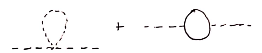
Figure 8: Diagrams giving the one-loop correction to the scalar propagator in Yukawa theory.

At one-loop, the scalar two-point function gets corrections due to both interactions, as seen in Figure 8. There is the diagram we had in the $\phi^{4}$ theory above, but we must recompute this in dim reg

$$i\Sigma_{\phi\text{ loop}}(p^{2}) =-i\frac{1}{2}\lambda\int\frac{d^{4}k}{(2\pi)^{4}}\frac{-i}{k^{2}+m^{2}}$$ (57)

$$=-i\frac{1}{2}\lambda\tilde{\mu}^{\epsilon}\int\frac{d^{d}\bar{k}}{(2\pi)^{d}}\frac{1}{\bar{k}^{2}+m^{2}}$$ (58)

$$=-i\frac{\lambda}{2}\Gamma\left(-1+\frac{\epsilon}{2}\right)\frac{m^{2}}{(4\pi)^{2}}\left(\frac{4\pi\tilde{\mu}^{2}}{m^{2}}\right)^{\epsilon/2}$$ (59)

$$\simeq i\frac{\lambda}{2(4\pi)^{2}}m^{2}\left(\frac{2}{\epsilon}+1-\gamma_{E}\right)\left(1+\frac{\epsilon}{2}\log\frac{4\pi\tilde{\mu}^{2}}{m^{2}}\right)$$ (60)

$$\simeq i\frac{\lambda}{2(4\pi)^{2}}m^{2}\left(\frac{2}{\epsilon}+1-\gamma_{E}-\log\frac{4\pi\tilde{\mu}^{2}}{m^{2}}\right)$$ (61)

$$=i\frac{\lambda}{(4\pi)^{2}}m^{2}\left(\frac{1}{2}+\frac{1}{\epsilon}+\frac{1}{2}\log\frac{\mu^{2}}{m^{2}}\right)+\mathcal{O}(\epsilon),$$ (62)

where we have analytically continued to $d=4-\epsilon$ dimensions including replacing $\lambda\mapsto\lambda\tilde{\mu}^{\epsilon}$, with $\tilde{\mu}$ a mass scale, to keep $\lambda$ dimensionless; performed the integral in general dimension; expanded for $\epsilon\simeq 0$; and defined $\mu^{2}\equiv 4\pi\tilde{\mu}^{2}e^{-\gamma_{E}}$, where $\gamma_{E}$ is the Euler-Mascheroni constant, to simplify the expression. Details on these calculational steps are laid out in Srednicki’s Chapter 14, but there’s an important and naïvely surprising feature of the above that we should discuss.

In previous sections our regularization scheme explicitly introduced a mass scale $\Lambda$ which we could think of as having a physical interpretation as some sort of short-distance cutoff, if we wished. We then saw that by cleverly studying how the parameters in the theory are modified as we change $\Lambda$ and demand the physics stays the same, we could make a variety of things easier to calculate and make the physical content of the theory more transparent. Note that in doing so, we’re stretching the meaning of the scale $\Lambda$ away slightly from that physical picture—we don’t care what the ‘real’ cutoff of our system is, or if there really is any sort of cutoff; we simply know that allowing such scale-dependence in our couplings and studying the theory at different values of $\Lambda$ makes our lives easier, so we imagine varying it.

Now the way this new regularization scheme works is somewhat opaque, but it still necessitates the introduction of a new scale. In this case, the unphysical scale $\mu$ is required to ensure that our couplings remain dimensionless away from $d=4$. This scheme thus invites us to further broaden our notion of varying a scale to study the theory at different energies—this time the scale explicitly never had a physical interpretation. We can view $\mu$ as labeling a one-parameter family of calculational schemes. We’ve ensured by construction that the physics is the same no matter what $\mu$ we choose, but by cleverly using the scale-dependence we can make our lives far easier. The intuition should be the same as in the previous case, and lowering $\mu$ does likewise transfer loop-level physics to tree-level physics and can be used to improve the convergence of perturbative calculations. The connection is now slightly more opaque, which is why we began by discussing a cutoff in Euclidean momentum space, but the calculations become far simpler.

There’s another diagram with a $\psi$ loop

$$i\Sigma_{\psi\text{ loop}}(p^{2}) =(-1)(ig)^{2}\int\frac{d^{4}k}{(2\pi)^{4}}(-i)^{2}\frac{\text{Tr}\left[(-\not{k}+M)\gamma_{5}(-\not{k}-\not{p}+M)\gamma_{5}\right]}{(k^{2}+M^{2})((k+p)^{2}+M^{2})}$$ (63)

$$=-\frac{g^{2}}{4\pi^{2}}\left[\frac{1}{\epsilon}(k^{2}+2M^{2})+\frac{1}{6}k^{2}+M^{2}-\int_{0}^{1}dx(3x(1-x)k^{2}+M^{2})\ln\frac{D}{\mu^{2}}\right],$$ (64)

with $D=x(1-x)k^{2}+m^{2}$, whose evaluation follows similar steps but we skip for brevity. Adding these together, $\overline{\text{MS}}$ tells us the $\phi$ counterterms must take the values

$$Z_{\phi} =1-\frac{g^{2}}{4\pi^{2}}\frac{1}{\epsilon}$$ (65)

$$Z_{m} =1+\left(\frac{\lambda}{16\pi^{2}}-\frac{g^{2}}{2\pi^{2}}\frac{M^{2}}{m^{2}}\right)\frac{1}{\epsilon}.$$ (66)

For the fermion, evaluating the one-loop diagrams gives us the counterterms

$$Z_{\psi} =1-\frac{g^{2}}{16\pi^{2}}\frac{1}{\epsilon}$$ (67)

$$Z_{M} =1-\frac{g^{2}}{8\pi^{2}}\frac{1}{\epsilon}.$$ (68)

Since we didn’t choose the counterterm to keep the location of the pole in the propagator fixed, $m$ is no longer the physical scalar mass. But we can find the physical, ‘pole’ mass precisely from that condition:

$$0 \equiv\Delta^{-1}(k^{2}=-m_{\text{phys}}^{2})$$ (69)

$$=\left.k^{2}+m^{2}+\Sigma(k^{2})\right|_{k^{2}=-m_{\text{phys}}^{2}}$$ (70)

$$=-m_{\text{phys}}^{2}+m^{2}-\Sigma(-m_{\text{phys}}^{2})$$ (71)

$$\Rightarrow m_{\text{phys}}^{2} =m^{2}-\Sigma(-m^{2})+\mathcal{O}(\lambda^{2},g^{4},\lambda g^{2}),$$ (72)

where we have used our favorite trick to replace $m_{\text{phys}}^{2}$ with $m^{2}$ in the one-loop correction, since it is already higher order in couplings.

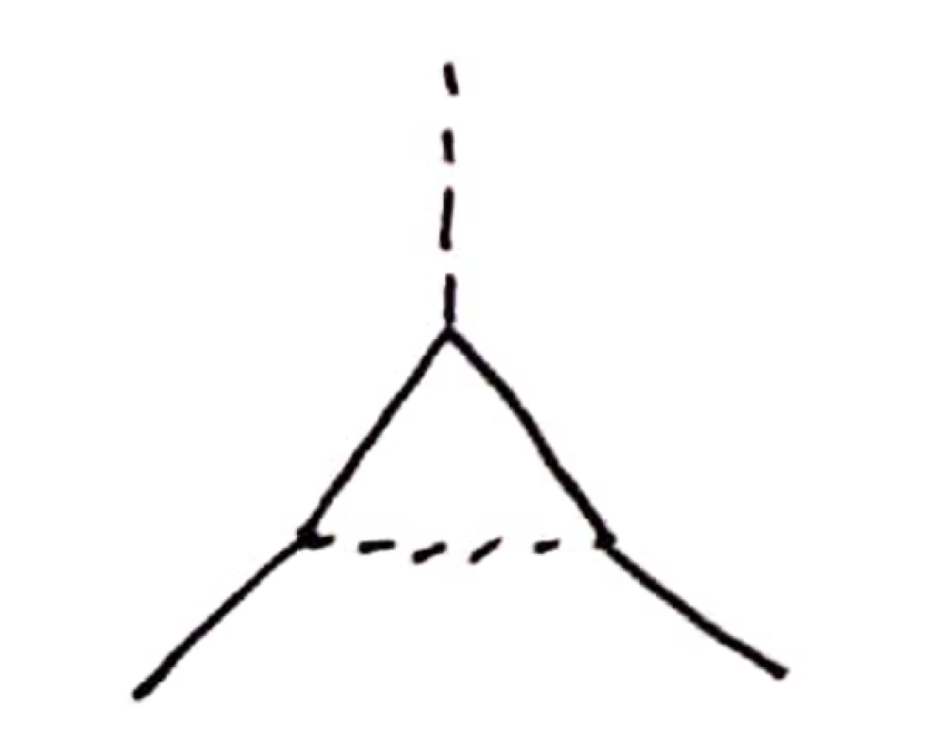
(a)

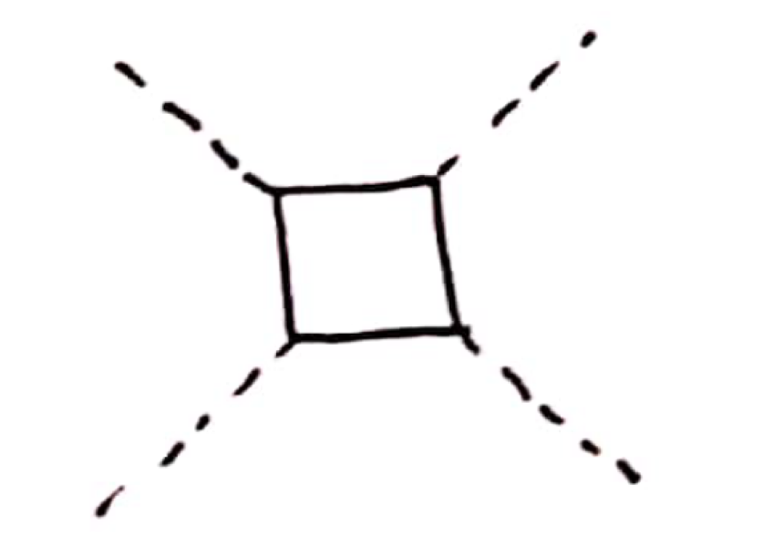
(b)

Figure 9: Some one-loop diagrams in Yukawa theory correcting the interactions. In (a), a triangle diagram correcting the Yukawa interaction. In (b), a box diagram correcting the scalar quartic interaction.

As for the interactions, we have a triangle diagram for the Yukawa coupling and a new contribution to the quartic with a fermion running in the loop, as depicted in Figures 9(a) and 9(b) respectively. These lead to the counterterms

$$Z_{g} =1+\frac{g^{2}}{8\pi^{2}}\frac{1}{\epsilon}$$ (73)

$$Z_{\lambda} =1+\left(\frac{3\lambda}{16\pi^{2}}-\frac{3g^{4}}{\pi^{2}\lambda}\right)\frac{1}{\epsilon},$$ (74)

from which we’ll be able to understand how the strength of the interactions changes as a function of the energy at which the theory is probed.

Renormalization group improvement

Now the second improvement to perturbation theory is the RG-improved perturbation theory we mentioned above. This takes on an even more useful role in our continuum renormalization scheme here. In the Wilsonian picture, $\Lambda$ was a high cutoff and we ensured the physics was invariant under evolution of $\Lambda$, but this scale still needed to stay far above the scales of interest in the problem $\Lambda\gg m,M,-k^{2},\dots$. Now the scale $\mu$ is entirely unphysical and we are free to bring it all the way down to the scales of kinematic interest—in fact doing so will vastly simplify calculations. As a result we are able to make even more use of the RG-improvement than we could above.

We find the running couplings by again using the fact that the bare parameters are independent of the unphysical renormalization scale $\mu$. Having utilized a mass-independent regulator, a Wilsonian interpretation of couplings running with the value of the regulator is nonsensical here and so renormalization group improvement is the way to extract predictions from this theory. We already have the relations between the bare and renormalized quantities, e.g.

$$g_{0}=Z_{\phi}^{-1/2}Z_{\psi}^{-1}Z_{g}g\tilde{\mu}^{\epsilon/2}.$$ (75)

And since we know that the bare parameters are independent of $\mu$ by definition, we have

$$\ln g_{0} =\ln\left(1+\frac{g^{2}}{8\pi^{2}}\frac{1}{\epsilon}\right)+\ln\left(1+\frac{g^{2}}{16\pi^{2}}\frac{1}{\epsilon}\right)+\ln\left(1+\frac{g^{2}}{8\pi^{2}}\frac{1}{\epsilon}\right)+\ln g+\frac{1}{2}\epsilon\ln\tilde{\mu}$$ (76)

$$=\frac{5g^{2}}{16\pi^{2}}\frac{1}{\epsilon}+\ln g+\frac{1}{2}\epsilon\ln\tilde{\mu}+\mathcal{O}(g^{4})$$ (77)

$$\frac{\text{d}\ln g_{0}}{\text{d}\ln\mu} =0$$ (78)

$$=\frac{10g}{16\pi^{2}}\frac{1}{\epsilon}\frac{\text{d}g}{\text{d}\ln\mu}+\frac{\text{d}\ln g}{\text{d}\ln\mu}+\frac{1}{2}\epsilon$$ (79)

$$=\frac{\text{d}g}{\text{d}\ln\mu}\left(1+\frac{5g^{2}}{8\pi^{2}}\frac{1}{\epsilon}\right)+\epsilon g.$$ (80)

If we expand $\frac{\text{d}g}{\text{d}\ln\mu}=a_{1}\epsilon+a_{0}+\dots$ order by order in $\epsilon$, then matching the $\mathcal{O}(\epsilon)$ terms gives $a_{1}=-g/2$ and matching the $\mathcal{O}(\epsilon^{0})$ terms tells us that, in the $\epsilon\rightarrow 0$ limit, we have

$$\frac{\text{d}g}{\text{d}\ln\mu}=\frac{5}{16\pi^{2}}g^{3}+\mathcal{O}(g^{4}).$$ (81)

This $\epsilon$-independent piece is known as the ‘beta function’ for the coupling, $\beta(g)=\frac{5}{16\pi^{2}}g^{3}$. Of course there are higher-order terms in $\frac{\text{d}g}{\text{d}\ln\mu}$ which are needed to match the $\mathcal{O}(\epsilon^{-n})$ terms, and which one can solve for. But these vanish in the $\epsilon\rightarrow 0$ limit, so will not contribute to the running of $g(\mu)$.

We can now resum this logarithm to find the evolution of this coupling with renormalization scale

$$g(\mu)=\frac{\bar{g}}{\sqrt[\ ]{1-\frac{5\bar{g}^{2}}{8\pi^{2}}\log\frac{\mu}{\bar{\mu}}}},$$ (82)

where we’ve used the boundary condition $g(\bar{\mu})=\bar{g}$. As before, the resummed version will allow us to maintain precision to far lower scale than we could with simply its leading order approximation.

It’s useful to keep in mind the Wilsonian picture as a clearer example because our regulator had a physical interpretation. The point is that the logarithms are really what’s encoding how couplings change as a function of scale; in the Wilsonian calculation it was obvious that the logarithmic contribution $\log\frac{1}{b}$ is present no matter the initial cutoff. One says that couplings which receive logarithmic quantum corrections ‘get contributions from all scales’. Then it’s clear why this RG-improvement is sensible—though we may start at some particular $\Lambda$ or $\mu$, a one-loop calculation offers information on the lowest-order logarithmic running over all momenta, and we may sum up those modifications to improve our perturbation theory.

3 To Relate Theories

Mass-independent schemes and matching

We’ve seen already the necessity of renormalization when a theory produces naïvely divergent results, and its enormous use in improving the precision of perturbative calculations in a given theory. The last facet we’ll discuss is its use in connecting theories. This is necessary to use the computationally-simple scheme of dim reg with $\overline{\text{MS}}$ in theories with different mass scales, and is very closely related to the effective field theory philosophy we discussed in Section 1. Cohen’s monograph [16] goes into far more depth than I will be able to, and is a fantastic introduction to these ideas and their application. This perspective on renormalization has also been of enormous use in condensed matter to understand behaviors that appear in many distinct systems in the long-distance limit, and has applications in formal field theory to understand better the properties of QFT itself.

In the previous section we derived the beta function for Yukawa theory in the $\overline{\text{MS}}$ scheme. As promised by our terming of this as a ‘mass-independent’ scheme, the beta functions indeed have no reliance on the masses. But this should seem remarkably peculiar, as it suggests that there is no decoupling at all. Were that the case, by measuring the low-energy beta functions of QED we could tell how many charged particles existed up to arbitrarily large mass scales! What has gone wrong is that $\overline{\text{MS}}$ does not meet the criterion of a physical scheme which is necessary for the Appelquist-Carrazone theorem to operate. In $\overline{\text{MS}}$ the renormalization condition has nothing to do with physical values of the parameters so, while it makes calculations far simpler, $\overline{\text{MS}}$ has broken decoupling.

To restore decoupling and allow us to properly use a mass-independent scheme, we must implement the mass-dependence ourselves by ‘matching’ the Yukawa theory at energies above the fermion mass to a theory of solely light scalars at energies below the spinor mass. To ‘match’, we consider some process which exists in both theories—for example, $\phi^{4}$ scattering—and ensure that at the matching scale $M$ both theories agree on the physics.

In the high-energy Yukawa theory we can run the RG scale all the way down from a high scale $\bar{\mu}$ to $\mu=M_{\text{phys}}$, the physical, pole mass of the fermion. To get simple closed-form expressions, we’ll take the couplings small enough that working to lowest order gives a good approximation. We’ll denote all of the UV values with bars, e.g. $M(\mu=\bar{\mu})=\bar{M}$. Firstly, we use the counterterms to find the anomalous dimension of the fermion mass

$$\frac{d\log M}{d\log\mu} =-\frac{d}{d\log\mu}\left(Z_{\psi}^{-1}Z_{M}\right)$$ (83)

$$=-\frac{g^{2}}{16\pi^{2}}$$ (84)

$$\Rightarrow M(\mu) \simeq\bar{M}\left(\frac{\bar{\mu}}{\mu}\right)^{\frac{\bar{g}^{2}}{16\pi^{2}}}$$ (85)

$$\simeq\bar{M}\left(1+\frac{\bar{g}^{2}}{16\pi^{2}}\log\frac{\bar{\mu}}{\mu}\right)+\dots$$ (86)

We then find the fermion pole mass as

$$0 =-M_{\text{phys}}+M(\mu=M_{\text{phys}})-\Sigma(-M_{\text{phys}})$$ (87)

$$M_{\text{phys}} =\bar{M}\left(1+\frac{\bar{g}^{2}}{16\pi^{2}}\log\frac{\bar{\mu}}{\bar{M}}\right)-\Sigma(-\bar{M})+\text{ subleading}$$ (88)

$$=\bar{M}\left(1+\frac{\bar{g}^{2}}{16\pi^{2}}\log\frac{\bar{\mu}}{\bar{M}}\right)-\frac{\bar{g}^{2}}{16\pi^{2}}\bar{M}\int_{0}^{1}dxx\log\left(\frac{x^{2}\bar{M}^{2}+(1-x)\bar{m}^{2}}{\bar{M}}\right)+\dots$$ (89)

$$=\bar{M}\left[1+\frac{\bar{g}^{2}}{16\pi^{2}}\left(\frac{1}{2}+\log\frac{\bar{\mu}}{\bar{M}}\right)\right]+\dots$$ (90)

Now we need the value of the other parameters at that mass threshold

$$\frac{1}{m}\frac{dm}{d\log\mu} =\frac{1}{4\pi^{2}}\left(\frac{1}{8}\lambda-g^{2}\frac{M^{2}}{m^{2}}+\frac{1}{2}g^{2}\right)$$ (91)

$$\Rightarrow m(M_{\text{phys}}) =\bar{m}\left(1-\frac{1}{4\pi^{2}}\left[\frac{1}{8}\bar{\lambda}-\bar{g}^{2}\frac{\bar{M}^{2}}{\bar{m}^{2}}+\frac{1}{2}\bar{g}^{2}\right]\log\frac{\bar{\mu}}{\bar{M}}\right)+\dots$$ (92)

$$\frac{dg}{d\log\mu} =\frac{5}{16\pi^{2}}g^{3}$$ (93)

$$\Rightarrow g(M_{\text{phys}}) =\bar{g}\left(1-\frac{5\bar{g}^{2}}{16\pi^{2}}\log\frac{\bar{\mu}}{\bar{M}}\right)+\dots$$ (94)

$$\frac{d\lambda}{d\log\mu} =\frac{1}{16\pi^{2}}\left(3\lambda^{2}+8\lambda g^{2}-48g^{4}\right)$$ (95)

$$\Rightarrow\lambda(M_{\text{phys}}) =\bar{\lambda}\left(1-\frac{1}{16\pi^{2}}\left[3\bar{\lambda}^{2}+8\bar{\lambda}\bar{g}^{2}-48\bar{g}^{4}\right]\log\frac{\bar{\mu}}{\bar{M}}\right)+\dots$$ (96)

Now we are ready to proceed to even lower energies. We enforce decoupling by matching to the low-energy theory of just a self-interacting scalar. We have

$$\mathcal{L}_{0} =\frac{1}{2}\phi\left(\Box-m^{2}\right)\phi$$ (97)

$$\mathcal{L}_{1} =-\frac{1}{24}Z_{\lambda}\lambda\phi^{4}+\mathcal{L}_{\text{ct}}$$ (98)

$$\mathcal{L}_{\text{ct}} =-\frac{1}{2}(Z_{\phi}-1)\partial^{\mu}\phi\partial_{\mu}\phi-\frac{1}{2}(Z_{m}-1)m^{2}\phi^{2}$$ (99)

The counterterms and beta functions in this theory can be conveniently found by truncating those found above. Of course, by construction, we find that the heavy fermion $\psi$ no longer contributes to the running of parameters at low-energies. To make sure we’re getting the physics correct, we must impose the boundary condition that the predictions match at $\mu=M_{\text{phys}}$, which here is quite simple—we just use the values at $M_{\text{phys}}$ in the UV theory as literal boundary conditions for our running in the IR theory. In the IR theory, for $\mu\leq M_{\text{phys}}$, we have

$$\frac{d\lambda}{d\log\mu} =\frac{3}{16\pi^{2}}\lambda^{2}$$ (100)

$$\Rightarrow\lambda(\mu) =\frac{\lambda(M_{\text{phys}})}{1+\frac{3}{16\pi^{2}}\lambda(M_{\text{phys}})\log\frac{M_{\text{phys}}}{\mu}}$$ (101)

$$\simeq\bar{\lambda}\left(1-\frac{1}{16\pi^{2}}\left[3\bar{\lambda}^{2}+8\bar{\lambda}\bar{g}^{2}-48\bar{g}^{4}\right]\log\frac{\bar{\mu}}{\bar{M}}\right)\left(1-\frac{3}{16\pi^{2}}\bar{\lambda}\log\frac{\bar{M}}{\mu}\right)+\dots$$ (102)

$$\simeq\bar{\lambda}\left(1-\frac{1}{16\pi^{2}}\left[3\bar{\lambda}^{2}+8\bar{\lambda}\bar{g}^{2}-48\bar{g}^{4}\right]\log\frac{\bar{\mu}}{\bar{M}}-\frac{3}{16\pi^{2}}\bar{\lambda}\log\frac{\bar{M}}{\mu}\right)+\dots$$ (103)

The benefit is now clear. While the RGEs in the UV theory were very complicated, the running of $\lambda$ in the low energy theory is simple. Our mass-independent scheme allows us to explicitly factorize these and contain all the UV physics in the boundary condition, which lets us study the low-energy theory in a simple manner.

The general procedure of renormalization group evolution in mass-independent schemes is called ‘running and matching’. The parameters in the Lagrangian run as you evolve down in energies, but at a mass threshold $M$ we must match the UV theory at $\mu=M$ from above to a theory without this field at $\mu=M$ from below. When we match we ensure that the physics of the low-energy fields stays constant as we cross that threshold and remove that particle from the spectrum of our theory. This becomes less trivial when we have multiple mass scales, so consider now upgrading our Yukawa theory with additional fermions.

$$\mathcal{L}\supset\sum\limits_{i=1}^{N}M_{i}\bar{\psi}_{i}\psi_{i}+g^{(N)}\phi\sum\limits_{i=1}^{N}\bar{\psi}_{i}\gamma_{5}\psi_{i}$$ (104)

Now if we are given the theory at very high energies $\mu\gg M_{i}$ and we want to understand what it looks like at very low energies, there is a cascade of EFTs we evolve through. As depicted in Figure 10, we run the parameters down to the largest fermion mass, match to a theory with one less fermion, run down again until the next mass scale, and so on.

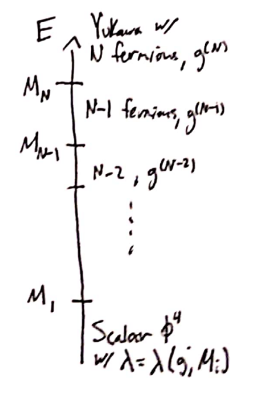
Figure 10: A schematic depiction of the cascade of effective field theories as one transitions from a Yukawa theory of $N$ fermions at high energies through integrating these out sequentially until one finds an effective $\phi^{4}$ theory at low energies.

As an example which is closer to the real world, consider QED with our three generations of leptons (and ignoring the strong sector for simplicity). At low energies we measure the asymptotic value $\alpha(\mu\simeq 0)\simeq 1/137$, and in colliders we measure the value of the gauge coupling at the $Z$ mass $m_{Z}\simeq 91\text{ GeV}$. To compare these, we must run the high-energy value all the way down into the infrared. Above $m_{\tau}\simeq 1.7\text{ GeV}$ we have a theory where all of $e,\mu,\tau$ run in loops and giving an $\overline{\text{MS}}$ beta function $\beta_{\alpha}=2\alpha^{2}/\pi$. But at $m_{\tau}$ we should remove the $\tau$ from our theory, such that from $m_{\tau}$ down to $m_{\mu}\simeq 105\text{ MeV}$ we have $\beta_{\alpha}=4\alpha^{2}/3\pi$. Below the $\mu$ we solely have the electron and recover the textbook $\beta_{\alpha}=2\alpha^{2}/3\pi$, and finally as we cross the electron mass threshold $m_{e}\simeq 511\text{ keV}$ we remove the electron from the spectrum and find that the gauge coupling stops running $\beta_{\alpha}\equiv 0$. Physically this corresponds to the fact that pure QED is scale-invariant, meaning that the coupling will not evolve at all in a theory with no charged particles. This is the regime in which classical electrodynamics holds precisely (up to the presence of additional interactions suppressed by powers of $m_{e}$, that is).

A possible confusion is to conflate the mass-independence of the regularization scheme with that of the renormalization scheme, and conclude that dimensional regularization cannot be used if one wants decoupling without having to integrate out and match. So lest one confuse the roles let’s quickly look at an example of using dimensional regularization with a renormalization scheme which does satisfy decoupling, known as ‘off-shell momentum subtraction’. For simplicity, we’ll look at the anomalous dimension of our Yukawa scalar $\phi$, and we’ll perform wavefunction renormalization by subtracting the value of the graphs at the off-shell momentum scale $k^{2}=\mu^{2}_{E}$. In symbols this amount to the prescription

$$Z_{\phi}=1+\Sigma_{\text{loop}}(k^{2}=\mu_{E}^{2}),\quad\text{ where }\Pi_{\text{loop}}(k^{2})=k^{2}\Sigma_{\text{loop}}(k^{2})+\text{ mass renorm pieces}.$$ (105)

Since we’re still using the same regularization scheme, we have the same result for $\Pi_{\text{loop}}(k^{2})$ as above. We can then simply calculate the anomalous scaling dimension as defined by $\gamma_{\phi}\equiv\frac{1}{2}\frac{\text{d}\log Z_{\phi}}{\text{d}\log\mu_{E}}$,

$$\gamma_{\phi} =\frac{1}{2}\frac{\text{d}\Sigma_{\text{loop}}(\mu_{E}^{2})}{\text{d}\log\mu_{E}}$$ (106)

$$=\frac{3g^{2}}{4\pi^{2}}\int\limits_{0}^{1}\text{d}x\frac{x^{2}(1-x)^{2}\mu_{E}^{2}}{M^{2}+(1-x)x\mu_{E}^{2}}.$$ (107)

This integral can be performed analytically, but the full expression is unilluminating. However, it is useful to look at the limits

$$\gamma_{\phi}=\begin{cases}\frac{g^{2}}{8\pi^{2}},&\mu_{E}^{2}\gg M^{2}\\ \frac{g^{2}}{40\pi^{2}}\frac{\mu_{E}^{2}}{M^{2}},&\mu_{E}^{2}\ll M^{2}\end{cases}$$

to check if they agree with our expectations. At energies far above the fermion mass its contribution to the scalar anomalous dimension cannot know about that scale, and at energies far below its mass we expect inverse dependence on the mass for decoupling to occur. This is precisely what we find, so the lesson is that even if we didn’t want to go through the trouble of integrating out the fermion and matching, we could still make use of the magical regularization scheme that is dim reg.

Flowing in theory space

Our interpretation of the renormalization group thus far has been as a way of understanding what a particular theory looks like at different energies. But there is another way of looking at it that is also useful, for which we shall follow an example of Peskin & Schroeder, though I recommend Skinner’s lecture notes [73] for clear explanation of these concepts which goes farther than we have time to. Let’s return to the idea of the Wilsonian path integral and successively integrating out Euclidean momentum shells. In the previous section we began with a scalar field theory

$$Z=\left(\int{\displaystyle\prod_{k=0}^{\Lambda}}\text{d}\phi(k)\right)\exp\left[-\int\text{d}^{d}x\left(\frac{1}{2}(\partial_{\mu}\phi)^{2}+\frac{1}{2}m^{2}\phi^{2}+\frac{1}{4!}\lambda\phi^{4}\right)\right].$$ (108)

We then integrated over momentum shells from $\Lambda$ down to $b\Lambda$ with $0<b<\Lambda$, and found we could express our result as (schematically; see 32,34,35,41)

$$Z =\left(\int{\displaystyle\prod_{k=0}^{b\Lambda}}\text{d}\phi(k)\right)\exp\left[-\int\text{d}^{d}x\mathcal{L}_{\text{eff}}\right]$$ (109)

$$\mathcal{L}_{\text{eff}} =\left(\frac{1}{2}(1+\Delta Z)(\partial_{\mu}\phi)^{2}+\frac{1}{2}(m^{2}+\Delta m^{2})\phi^{2}+\frac{1}{4!}(\lambda+\Delta\lambda)\phi^{4}+\frac{1}{6!}\Delta c_{6}\phi^{6}+\dots\right).$$ (110)

Above we interpreted this in terms of looking at the same theory at lower energies, having coarse-grained over the largest momentum modes, which is a useful way of comparing the two path integrals. Another useful way to compare is to get them to a form where they look similar, so let’s now define a change of variables $k^{\prime}=k/b,x^{\prime}=xb$, in terms of which the path integral now looks like

$$Z =\left(\int{\displaystyle\prod_{k^{\prime}=0}^{\Lambda}}\text{d}\phi(k^{\prime})\right)\exp\left[-\int\text{d}^{d}x^{\prime}\mathcal{L}_{\text{eff}}\right]$$ (111)

$$\mathcal{L}_{\text{eff}} =b^{-d}\left(\frac{1}{2}(1+\Delta Z)b^{2}(\partial_{\mu^{\prime}}\phi)^{2}+\frac{1}{2}(m^{2}+\Delta m^{2})\phi^{2}+\frac{1}{4!}(\lambda+\Delta\Lambda)\phi^{4}+\frac{1}{6!}\Delta c_{6}\phi^{6}+\dots\right).$$ (112)

We can transform the kinetic terms back to the canonical form with the field redefinition $\phi^{\prime}(x^{\prime})=b^{(2-d)/2}(1+\Delta Z)^{1/2}\phi(x^{\prime})$, after which we can write the effective Lagrangian as

$$\mathcal{L}_{\text{eff}}=\frac{1}{2}(\partial_{\mu^{\prime}}\phi^{\prime})^{2}+\frac{1}{2}m^{\prime 2}\phi^{\prime 2}+\frac{1}{4!}\lambda^{\prime}\phi^{\prime 4}+\frac{1}{6!}c^{\prime}_{6}\phi^{\prime 6}+\dots.$$ (113)

with $m^{\prime 2}=(m^{2}+\Delta m^{2})(1+\Delta Z)^{-1}b^{2},\ \lambda^{\prime}=(\lambda+\Delta\lambda)(1+\Delta Z)^{-2}b^{d-4},\ c_{6}^{\prime}=\Delta c_{6}(1+\Delta Z)^{-3}b^{2d-6},\dots$, and it’s clear that we could write such an effective action regardless of what sort of coefficients we began with before integrating out this momentum shell.

Now our series of transformations has effected the change (up to normalization)

$$Z=\left(\int{\displaystyle\prod_{k=0}^{\Lambda}}\text{d}\phi(k)\right)\exp\left[-\int\text{d}^{d}x\mathcal{L}\right]\rightarrow Z=\left(\int{\displaystyle\prod_{k^{\prime}=0}^{\Lambda}}\text{d}\phi^{\prime}(k^{\prime})\right)\exp\left[-\int\text{d}^{d}x^{\prime}\mathcal{L}^{\prime}\right].$$ (114)

Since all of our dynamical variables are integrated over in calculating the partition function, we can view this as a transition in the space of Lagrangians, $\mathcal{L}\rightarrow\mathcal{L}^{\prime}$. So this gives us an interpretation of the renormalization group as a flow in ‘theory space’.

This interpretation invites us to conceptualize renormalization group flow as a path through theory space between two conformal field theories (CFTs), as depicted in Figure 11. CFTs are quantum field theories with an enlarged spacetime symmetry group, consisting essentially of a scaling symmetry. CFTs are fixed points of RG flows—since they possess scaling symmetry they look the same at all energy scales, so if an RG flow is to have an endpoint it clearly must be a CFT.

There’s a terminological confusion here, which is that the ‘renormalization group’ isn’t actually a group at all, since the operation of integrating out a momentum shell is irreversible. This came up already above when we saw that integrating out heavy fields means we can no longer compute processes which have them as external fields (see Footnote 1). Flowing to lower energies, or toward the IR, is really a coarse-graining operation which does lose information about small scales, in precise analogy to decreasing the resolution of an image. This means that RG evolution is a directed flow, so there is a difference between fixed points in the UV and in the IR.

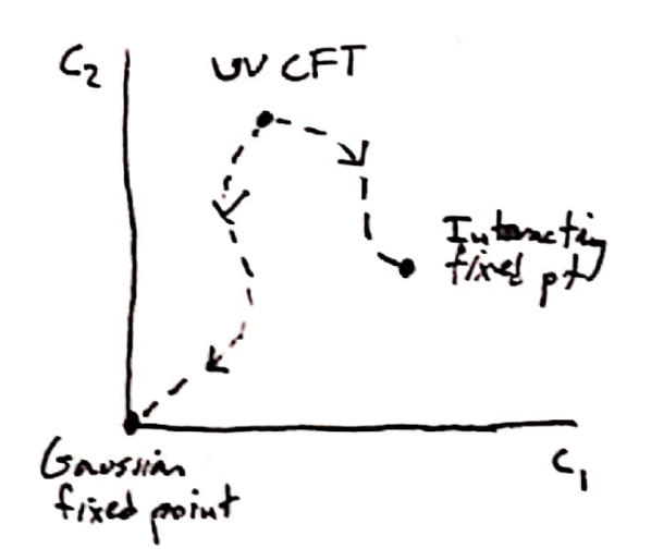
Figure 11: Schematic two-dimensional projection of some RG flow trajectories from an interacting UV fixed point which has been perturbed by one or another relevant operator, and which flow to IR fixed points that are either interacting or free. Perturbing the UV CFT by an irrelevant operator would lead to a flow directly back to the same CFT.

Quantum field theories can have different sorts of fixed points. As a familiar example, if the theory has a ‘mass gap’—no zero-energy excitations in the infrared, which may be because one began solely with massive fields or through dynamical mechanisms like Higgsing and confinement—then one finds a ‘trivial’ fixed point. In the far infrared, everything has been integrated out and there is not enough energy to excite any modes. We know phenomenologically that this happens in QCD. In the other familiar case one can have a ‘Gaussian’ or ‘free’ fixed point if the theory contains massless fields which don’t interact, such as in QED. At energies far below the mass of the lightest charged particle this is a theory of free electromagnetism, though one can still excite photons of arbitrarily-long wavelength.

Such a Gaussian fixed point occurs in the UV for QCD—the celebrated result of ‘asymptotic freedom’ [77, 78]—because the strong coupling flows toward zero, giving a free theory. This famously cannot occur for $U(1)$ gauge theories whose couplings necessarily grow with increasing energies, leading them to herald their own breakdown with the prediction of a ‘Landau pole’ [79], a finite UV energy where the perturbative theory predicts the coupling becomes infinite. From one perspective this is an inverse to the prediction of a confinement scale in QCD, where the perturbative prediction is a blowup of the coupling at low energies, as we’ll discuss further in Section 3. In either case the theory cannot make predictions for energies above the Landau pole or below the confinement scale, respectively, and so can be called inconsistent.

It’s clear that the divergence of a coupling either in the IR or the UV is problematic for a complete, consistent interpretation of a QFT. This is precisely why the formal perspective on a well-defined QFT is that it describes an RG flow between two CFTs, such that in neither direction does a coupling grow uncontrollably. In fact this provides an incredibly important perspective on renormalizability, which we’ll get to momentarily.

First, let us introduce somewhat of a generalization of the ‘relevant/irrelevant’ terminology which we introduced in Section 1. We implicitly had in mind that we were studying a theory in the vicinity of the Gaussian fixed point which we perturbed with various field operators—indeed, this is precisely how we normally carry out perturbative calculations—and our terminology depended on that. Generally one wishes to imagine perturbing a CFT by a particular operator, flowing down in energy, and seeing whether the operator grows in importance—a relevant operator—or shrinks—an irrelevant operator. Perturbing a CFT by an irrelevant operator does not induce an RG flow (to a different CFT), so interesting dynamical RG flows come from CFTs perturbed by relevant operators. This clearly agrees with our power-counting notion of relevance when we’re near the Gaussian fixed point, but works also if one is near a strongly-coupled, interacting fixed point where one may not know how to do such power-counting and anomalous dimensions of operators may grow to overpower their classical dimensions.

The importance of this language was realized in particular by Polchinski in his pioneering article [21]. He showed that in fact the intuitive notion of ‘power-counting renormalizability’ that the field had been building—that for a theory near the Gaussian fixed point we could see whether it was renormalizable merely by checking whether it has any coefficients of negative mass dimensions—in fact maps on to a very general statement. This is enormously powerful, as prior arguments for renormalizability were made on a case by case basis and were complicated and messy and graph-theoretic. His derivation of this fact is brilliant but requires much work, so we’ll merely try to get a sense for why it should be true by building on our intuition from our Wilsonian renormalization of $\phi^{4}$ theory in Section 1.

So long as your theory has a finite number of fields, all of which have mass dimension $\left[\phi_{i}\right]>0$ when canonically normalized, then there are a finite number of relevant or marginal operators. As we flow down in energy through theory space, we saw above the sense in which those coefficients are UV-sensitive—the IR coefficients of those operators are determined primarily by their UV values and IR corrections are subdominant. Contrariwise, the coefficients of the infinite number of possible irrelevant operators are UV-insensitive, being determined primarily by the IR physics of the relevant and marginal operators. That is, the RG flows are attracted to a finite-dimensional submanifold of the space of Lagrangians.

Consider a Wilsonian RG flow where we start off, as above, by specifying a cutoff $\Lambda_{0}$ and the values of coefficients $\lambda_{0}^{i}$ of all the $n$ marginal and relevant operators at that scale, as well as the coefficients $c_{0}^{i}$ of however many irrelevant operators we wish to turn on. We can then flow downwards in energy as normal, and at an energy scale $\Lambda_{R}\ll\Lambda_{0}$ let’s say we measure the relevant and marginal coefficients $\lambda_{R}^{i}$ at that scale. The coefficients of the irrelevant operators are then dominated by the infrared $\lambda_{R}^{i}$ and $\Lambda_{R}$ up to precision $(\Lambda_{R}/\Lambda_{0})^{\Delta_{i}}$ from subleading corrections, with $\Delta_{i}>0$ the scaling dimension of the irrelevant operator. So indeed, the RG flow is attracted to the $n$-dimensional surface described by $c_{i}=c_{R}^{i}(\lambda_{R}^{i};\Lambda_{R})$ and separate trajectories through theory space as a function of scale $\Lambda$ which reach the same $\lambda_{R}^{i}$ will differ only by positive powers of $(\Lambda_{R}/\Lambda_{0})$. For less abstract discussion, Polchinski goes through a simple example which may provide further insight, and Schwartz discusses the same example in Chapter 23 of his textbook [22].

To see why this implies renormalizability, recall that the program of Wilsonian renormalization is to define renormalized, ‘running’ couplings as a function of scale to keep infrared physics at $\Lambda_{R}$ fixed while ‘removing the cutoff’. A bit more formally, we want a family of Lagrangians $\mathcal{L}(\Lambda_{0};\lambda_{0}^{i},c_{0}^{i})$ with coefficients chosen as a function of $\Lambda_{0}$ such that each Lagrangian yields the same low energy physics $\lambda_{R}^{i}$, in terms of which all the IR observables can be calculated up to subleading corrections in $\Lambda_{R}/\Lambda_{0}$. When the cutoff is removed by taking $\Lambda_{0}\rightarrow\infty$, one thus recovers precisely the correct physics, specified by those chosen values of the $\lambda_{R}^{i}$, which are the renormalization conditions. If we can find such a family of Lagrangians, then we say this theory is power counting renormalizable. Polchinski’s argument shows that this can be done so long as one wishes solely to fix the IR values of relevant and marginal couplings.

Trivialities

The attentive reader may at this point notice an inconsistency due to imprecise language. We’ve seen now that the criterion for renormalizability, which Polchinski provided a robust basis for, is power-counting of the operators near the IR fixed point. This would suggest that the $\lambda\phi^{4}$ theory we’ve studied by means of an example is renormalizable. However, recall the result of resumming its renormalization group equation:

$$\lambda(\Lambda)=\frac{\lambda(\Lambda_{0})}{1+\frac{3\lambda(\Lambda_{0})}{16\pi^{2}}\log\frac{\Lambda_{0}}{\Lambda}},$$ (115)

which has a Landau pole for $\Lambda=\Lambda_{0}\exp(\frac{16\pi^{2}}{3\lambda(\Lambda_{0})})$, preventing us from taking the limit we required above. A mathematical physicist would say $\lambda\phi^{4}$ theory is ‘trivial’ or ‘quantum trivial’, as if we demand the existence of a continuum limit, that sets $\lambda(\Lambda)=\lambda(\Lambda_{0})=0$.

The issue is that the tree-level, classical scaling dimension captures only the scaling of the operators infinitesimally close to the infrared Gaussian fixed point. If we move a finite distance upward in energy scale, we’ve seen above that the $\phi^{4}$ operator gets an anomalous dimension $\delta_{\phi^{4}}>0$ and so is marginally irrelevant. So it’s clear that Polchinski’s picture of renormalization is only getting at a perturbative sense of renormalizability, and cannot tell us whether there truly exists an RG flow from a UV fixed point down to the IR theory we want to study.

So what are we to make of $\lambda\phi^{4}$ theory—or for that matter of QED, which has the same problem? Of course we know empirically that QED works fantastically well and we can absolutely make finite, accurate predictions after a finite number of inputs. To understand this, we must appeal the language of effective field theory, which we’ve already discussed. In fact the feature we’re really relying on is effective renormalizability, which tells us we require solely a finite number of inputs to set the behavior of the theory to a given precision. It’s clear that in this sense QED itself is an effective field theory whose validity breaks down somewhere below its Landau pole.

Finally, let me mention another reason not to be too worried that our most beloved quantum field theories don’t exist in the continuum limit: Our universe is not described by a QFT at its smallest scales! It’s indeed true that only RG flows between a UV CFT and an IR CFT can hope to define fully consistent and mathematically well-defined QFTs. But the existence of gravity—and the very strong evidence that a quantum field theory of gravity is inconsistent—means that at some energy scale effects not present in quantum field theory must become relevant. And since gravity couples universally to everything [80, 81], we have no strict empirical need for a UV complete, interacting quantum field theory that does not include gravity. It is entirely consistent, and overwhelmingly likely, that a quantum-field-theoretic description of the world works only approximately and some inherently quantum gravitational theory provides a sensible UV complete theory.

4 To Reiterate

Before moving on, let us reiterate what we’ve discussed about renormalization. As we’ve seen, renormalization is so important and so useful and fulfills so many purposes that an entirely general statement risks becoming vague. But if a single sentence summary is demanded: Renormalization reveals for us the scale-dependence of a quantum mechanical field theory.

The effects of this seemingly innocuous statement, however, are powerful and manifold, including:

• Correctly accounting for this scale-dependence is necessary to have well-defined quantum field theories, which otherwise appear nonpredictive.

• Bringing the non-scale-invariance of the quantum mechanical theory into clear scale-dependence of the couplings makes it simple to read off the qualitative behavior at different scales from the renormalized Lagrangian.

• Including this scale-dependence in the couplings allows us to reorganize our perturbative series such that we can efficiently calculate the behavior of the theory over a far wider range of energies than a naïve treatment allows.

• Properly accounting for the scale dependence allows us to harness the full power of effective field theory, as we can study a theory of low-energy fields which correctly accounts for corrections from the high-energy physics.

• Understanding the perspective of single quantum field theories as flows through theory space as a function of the scale allowed us to develop a nonperturbative definition of a fully UV-complete quantum field theory and how it behaves.

All of these various perspectives will be of use in the following chapters as we apply this technology to understanding what the hierarchy problem is and how we can solve it.

3 Naturalness

Naturalness is the notion that we have the right to ask about the origins of the dimensionless numbers in our theories—past solely fitting them to the data. It was Dirac who first introduced such a notion to particle physics in 1938 [82]. In modern language, what is referred to as ‘Dirac naturalness’ consists of the idea that dimensionless parameters in a fundamental physical theory should take values of order 1. In the language of EFT, in a theory with a cutoff $\Lambda$ and an operator $O$ with scaling dimension $\Delta$, we expect its coefficient to take a value $c_{O}\sim\mathcal{O}(1)\Lambda^{d-\Delta}$. As stated this is essentially dimensional analysis, as $\Lambda$ is the only scale we’ve introduced, but we will discuss below that quantum mechanics gives additional credence to this expectation—indeed we’ve already seen this feature in our one-loop examples above.

’t Hooft pointed out a refinement of this principle [83], which has come to be called ‘technical naturalness’. If the operator $O$ breaks a symmetry which is respected by the action in the limit $c_{O}\rightarrow 0$, then one says it is ‘technically natural’ for $c_{O}$ to take on a small value. The reasoning here is simple—as we saw above, in a quantum field theory defined at a high scale, one finds corrections $\delta c_{O}$ to such coupling constants as they run to low energies. If there is an enhanced symmetry of the theory in the limit that $c_{O}\rightarrow 0$, then such quantum mechanical corrections cannot generate that operator and break the symmetry, so we know that $\delta c_{O}\propto c_{O}$. The low-energy effective field theorist says of such couplings that one can ‘set it and forget it’: if one has $c_{O}\ll 1$ at the cutoff $\Lambda$, that coupling will remain small as one flows to lower energies.

Conversely, we can emphasize the connection to Dirac naturalness by looking at this picture in reverse. We know of mechanisms to generate small technically natural couplings at low energies from Dirac natural ones, as we will discuss in detail below. Imagine one measures a small coupling $c_{O}$ at long distances in the low-energy theory with cutoff $\Lambda$ that does not have a Dirac natural explanation. If that parameter is technically natural, it remains small up to the cutoff, and so the next generation of physicists can explain its small size at $\Lambda$ in the UV theory, as emphasized nicely by Zhou [84]. If $c_{O}$ is not technically natural, then its RG evolution up to the cutoff yields a value to which the low-energy physics is very sensitive, and we must explain why it has a very specific value such that the correct physics emerges at long distances.

1 Technical Naturalness and Fine-Tuning

A model is fine-tuned if a plot of the allowed parameter space makes you wanna puke.

David E. Kaplan (2007)

It’s useful to make this less abstract by looking at a simple example. Consider a $d=6$ dimensional effective field theory of a real scalar field $\phi$ of mass $m$ which is odd under a $\mathbb{Z}_{2}$ symmetry, which we expect is a good description of our system up to a cutoff $\Lambda$ with $m\ll\Lambda$. If we add a small explicit breaking $\sigma\phi^{3}$ with $\sigma\ll 1$ at low energies, $\sigma$ is technically natural and stays small up to the cutoff, so we can easily write down a UV completion which generates this small value Dirac naturally.

However, if we add another $\mathbb{Z}_{2}$-odd real scalar $\Phi$ and give it a large $\mathbb{Z}_{2}$-breaking interaction with $\phi$, then $\sigma$ is no longer technically natural. Its low-energy value becomes extremely sensitive to the values of the parameters at the cutoff. It then becomes difficult to understand an ultraviolet reason for why those values take the precise values they need to realize small $\sigma$ in the far IR. Consider the bare action

$$S=\int\text{d}^{6}x\left[-\frac{1}{2}(\partial\phi_{0})^{2}-\frac{1}{2}m_{0}^{2}\phi_{0}^{2}-\frac{1}{2}(\partial\Phi_{0})^{2}-\frac{1}{2}m_{0}^{2}\Phi_{0}^{2}-\frac{\sigma_{0}}{3!}\phi_{0}^{3}-\frac{y_{0}}{2}\phi_{0}\Phi_{0}^{2}\right],$$ (116)

where we’ve given the two fields the same mass for simplicity. This is not stable under radiative corrections, but that’s a higher-order effect which will not come into our one-loop calculation of the RG evolution of the cubic couplings.

We will renormalize this theory at one loop using dim reg with $\overline{\text{MS}}$. As discussed above, we will compute the one-loop 1PI diagrams and add counterterms to cancel solely the $\frac{1}{\epsilon}$ pieces of the results. With counterterms, the action is

$$S=\int\text{d}^{d}x\left[-\frac{1}{2}Z_{\phi}(\partial\phi)^{2}-\frac{1}{2}Z_{m\phi}m^{2}\phi^{2}-\frac{1}{2}Z_{\Phi}(\partial\Phi)^{2}-\frac{1}{2}Z_{m\Phi}m^{2}\Phi^{2}+\frac{\sigma}{3!}Z_{\sigma}\phi^{3}+\frac{y}{2}Z_{y}\phi\Phi^{2}\right]$$ (117)

where these parameters and fields are the renormalized parameters, and for compactness we have not written down the split of these terms as we did above in Equation 97. At tree level the relation to the bare quantities is trivial and so $Z=1+\dots$. To get an accurate picture of how the strength of the interactions vary as they’re probed at different energy scales, we must fully renormalize the theory. Since our focus is on the interactions, we simply state the results for the quadratic part of the action, where we have

$$Z_{\phi} =1-\frac{1}{6(4\pi)^{3}}\left(\sigma^{2}+y^{2}\right)\frac{1}{\epsilon}+\dots$$ (118)

$$Z_{\Phi} =1-\frac{1}{3(4\pi)^{3}}\left(\sigma^{2}+y^{2}\right)\frac{1}{\epsilon}+\dots$$ (119)

$$Z_{m\phi} =1-\frac{1}{(4\pi)^{3}}\left(\sigma^{2}+y^{2}\right)\frac{1}{\epsilon}+\dots$$ (120)

$$Z_{m\Phi} =1-\frac{2}{(4\pi)^{3}}y^{2}\frac{1}{\epsilon}+\dots$$ (121)

These tell us that the physical mass of the fields and the normalization of their one-particle states has changed. The relation to these can be found using the quantum-corrected propagator $\Delta(k^{2})^{-1}$ as $\Delta(-m_{\text{phys}}^{2})^{-1}\equiv 0$ to define the mass and $R^{-1}=\left.\frac{d}{dk^{2}}\left[\Delta(k^{2})^{-1}\right]\right|_{k^{2}=-m_{\text{phys}}^{2}}$ to define the normalization $R$, but solving for these relations explicitly will not be necessary for our purposes.

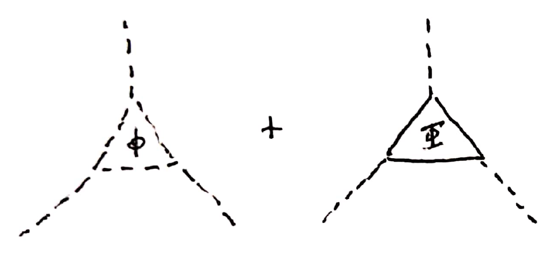
(a)

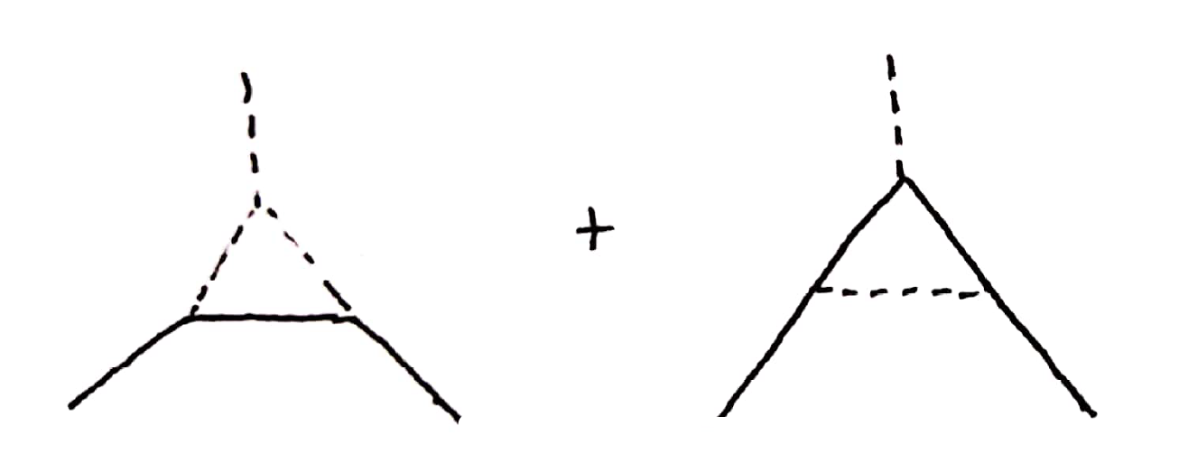
(b)

Figure 12: Diagrams contributing to the one-loop corrections to the three-point functions in our $6d$ scalars with cubic interactions. Dashed lines denote $\phi$ and full lines denote $\Phi$. In (a), the diagrams renormalizing $\sigma$, and in (b), the diagrams renormalizing $y$.

The one-loop three-point functions each have two diagrams, whose evaluation only differs in the coupling constants. For the correction to $\sigma$, we have triangle diagrams with either $\phi$ or $\Phi$ running in the loop. We can evaluate them in $d=6-\epsilon$ dimensions as

$$i\frac{1}{\sigma}V_{\sigma} =\frac{1}{\sigma}\left[(i\sigma)^{3}+(iy)^{3}\right]\int\frac{d^{6}q}{(2\pi)^{6}}\frac{(-i)^{3}}{(q^{2}+m^{2})^{3}}$$ (122)

$$=\frac{i}{\sigma}\left[\sigma^{3}+y^{3}\right]\tilde{\mu}^{\epsilon}\int\frac{d^{d}\bar{q}}{(2\pi)^{d}}\frac{1}{(\bar{q}^{2}+m^{2})^{3}}$$ (123)

$$=\frac{i}{\sigma}\left[\sigma^{3}+y^{3}\right]\tilde{\mu}^{\epsilon}\frac{\Gamma\left(\frac{\epsilon}{2}\right)}{2(4\pi)^{3}}\left(\frac{m^{2}}{4\pi}\right)^{-\frac{\epsilon}{2}}$$ (124)

$$=\frac{i}{2(4\pi)^{3}\sigma}\left[\sigma^{3}+y^{3}\right]\left(\frac{2}{\epsilon}-\gamma_{E}\right)\left(1+\frac{\epsilon}{2}\log\frac{4\pi\tilde{\mu}^{2}}{m^{2}}\right)$$ (125)

$$=\frac{i}{2(4\pi)^{3}\sigma}\left[\sigma^{3}+y^{3}\right]\left(\frac{2}{\epsilon}+\log\frac{\mu^{2}}{m^{2}}\right).$$ (126)

The counterterm vertex contributes to this as $-i(Z_{\sigma}-1)$, meaning that $\overline{\text{MS}}$ prescribes we set

$$Z_{\sigma}=1+\frac{1}{(4\pi)^{3}}\left(\sigma^{2}+\frac{y^{3}}{\sigma}\right)\frac{1}{\epsilon}$$ (127)

For the other vertex correction there are diagrams with either one or two of each internal line, which give

$$i\frac{1}{y}V_{y} =\frac{1}{y}\left[(iy)^{3}+(i\sigma)(iy)^{2}\right]\int\frac{d^{6}q}{(2\pi)^{6}}\frac{(-i)^{3}}{(q^{2}+m^{2})^{3}}$$ (128)

$$=\frac{i}{2(4\pi)^{3}}\left[y^{2}+\sigma y\right]\left(\frac{2}{\epsilon}+\log\frac{\mu^{2}}{m^{2}}\right),$$ (129)

leading to the counterterm

$$Z_{y}=1+\frac{1}{(4\pi)^{3}}\left(y^{2}+\sigma y\right)\frac{1}{\epsilon}.$$ (130)

This gives us the beta functions

$$\beta_{\sigma} =\frac{1}{4(4\pi)^{3}}\left(-3\sigma^{3}-4y^{3}+y^{2}\sigma\right)+\dots$$ (131)

$$\beta_{y} =\frac{1}{12(4\pi)^{3}}\left(\sigma^{2}y-12\sigma y^{2}-7y^{3}\right)+\dots$$ (132)

Now we are finally in a place to mathematically evince our physics point about technical naturalness. Without $\Phi$, the coupling $\sigma$ is the only one which violates the $\mathbb{Z}_{2}$ and so the beta function is necessarily proportional to $\sigma$. Let’s say we recruit an experimentalist friend of ours to measure the $2\rightarrow 2$ scattering cross-section of $\phi$s and we find that at $\mu=m$, the theory fits the data for $\sigma(m)=\sigma_{0}$ with $\sigma_{0}\ll 1$. Solving the beta function, we find that to lowest order

$$\sigma(\mu)\simeq\sigma_{0}\left(1-\frac{3}{4(4\pi)^{3}}\sigma_{0}^{2}\log\left[\frac{\mu}{m}\right]\right).$$ (133)

So $\sigma$ is indeed radiatively stable. If $\sigma(m)=\sigma_{0}$ is small, then it takes until the enormous scale $\mu\simeq m\exp\left((4\pi)^{3}/\sigma_{0}^{2}\right)$ for $\sigma$ to change by an order one fraction. So running $\sigma(\mu)$ up to wherever the cutoff $\Lambda$ of our theory is, $\sigma(\Lambda)$ will still be small. If by $\Lambda$ we haven’t discovered any explanation for the size of $\sigma(m)$, we can ask the theory above $\Lambda$ to produce this small value of $\sigma(\Lambda)$ from Dirac natural parameters at yet higher energies. Perhaps the high-energy Dirac natural value of $\sigma$ has been relaxed toward zero by an axion-type mechanism, or perhaps $\sigma$ is the vev of another $\mathbb{Z}_{2}$-odd field which spontaneously broke the $\mathbb{Z}_{2}$ via confinement. We don’t need to know a particular mechanism; the fact that $\sigma$ is technically natural means that if we don’t find an explanation for its size there is hope yet that our academic descendants will. One says that here $\sigma$ is UV-insensitive as its low-energy value does not depend strongly on the physics at high energies.

On the other hand, if $\sigma$ is not technically natural, we have a much more difficult issue. If we now have the theory with both $\phi$ and $\Phi$, and our experimentalist measures $\sigma(m)=\sigma_{0}\ll 1$ and $y(m)=y_{0}=\mathcal{O}(1)$, then to lowest order the RG evolution of $\sigma$ will be $\beta_{\sigma}\simeq-y^{3}/(4\pi)^{3}$ leading to

$$\sigma(\mu)=\sigma_{0}-\frac{1}{(4\pi)^{3}}y_{0}^{3}\log\left[\frac{\mu}{m}\right].$$ (134)

And we can see the issue, as we are no longer guaranteed that a small $\sigma(m)$ is related to a small $\sigma(\Lambda)$. For concreteness, if $\sigma_{0}=10^{-3}$, $y_{0}=-5$ and $\Lambda=10^{5}m$, then (using the full one-loop RG), we have $\sigma(\Lambda)\simeq 0.55$ and $y(\Lambda)\simeq 4.16$. How are we to ensure these values at $\Lambda$? We know how to produce small numbers, but not incredibly specific ones.

To see that we do need to produce these values very precisely, let’s switch directions and consider the RG evolution down in energy from $\Lambda$ to $m$. In the theory with solely $\phi$, the coupling $\sigma$ runs incredibly slowly, so an $\mathcal{O}(1)$ change in $\sigma(\Lambda)$, evolved down to the scale $m$, results in an $\mathcal{O}(1)$ change to $\sigma(m)$. But in the theory with two sources of breaking, $\sigma(m)$ is enormously sensitive to the values of the couplings at $\Lambda$. With the same cutoff $\Lambda=10^{5}m$, if we very slightly change the input value to $\sigma(\Lambda)=0.56$ and leave $y(\Lambda)$ as above, evolving down now gives us $\sigma(m)\simeq 10^{-2}$—a $<2\%$ change in input parameters has resulted in a $1000\%$ change in our low energy observable! It’s even more sensitive to the input value of $y$; a $\sim 1\%$ modification solely to $y(\Lambda)=-4.20$ trickles down to give $\sigma(m)\simeq 2\times 10^{-{2}}$, a $2000\%$ change. In this theory $\sigma$ is now a UV-sensitive parameter, whose low-energy behavior depends strongly on the high-energy physics. To say the least, it seems difficult to find a natural way to achieve the precise values needed to reproduce the observed low-energy physics in this theory. We’ll return to this issue at length in Section 2.

Technical naturalness and masses

Our understanding of technical naturalness allows us to already see another warning sign of the hierarchy problem. An elementary spin-1 field comes along with a gauge symmetry $A^{\mu}\rightarrow A^{\mu}-\partial^{\mu}\alpha(x)$ which is broken by a mass term $m_{A}^{2}A^{\mu}A_{\mu}$. So a mass for a gauge boson is technically natural and one necessarily finds $\delta m_{A}^{2}\propto m_{A}^{2}$. Similarly, a massive Dirac fermion $\Psi=(\psi,\chi^{\dagger})$ has a $U(1)$ global symmetry under which $\psi\rightarrow e^{i\alpha}\psi,\chi\rightarrow e^{-i\alpha}\chi$. In the $m\rightarrow 0$ limit, the symmetry is enhanced to $U(1)^{2}$ as arbitrary rephasings of the two Weyl fermions become symmetries, so again $\delta m_{\Psi}\propto m_{\Psi}$. But an elementary scalar does not automatically come with any such protective symmetry, and we’ve already seen in all our examples above that scalar mass corrections indeed get contributions not proportional to the mass itself.

In fact for discussing the technical naturalness of masses there is an even simpler argument: A massless spin-1 boson has two degrees of freedom and a massive one has three. Quantum corrections cannot generate a degree of freedom ex nihilo, so a massless gauge boson must be protected. Similarly a massless chiral fermion has two degrees of freedom, but a massive Dirac fermion has four. So for charged spinors and for vectors, it is simply the representation theory of the Lorentz group that is responsible for the stability of their masses. In either of these cases mass must arise from interactions of the field with a scalar (very broadly defined) as in the Higgs mechanism, which can pair up chiral spinors together and lend vectors another degree of freedom. But a massless scalar and a massive scalar have the same number of degrees of freedom. If we want a scalar mass to be technically natural, it must come from some symmetry past simply the Lorentz group. We’ll see some examples of how to arrange this in Chapter 2.

2 Spurion Analysis

An important tool for understanding symmetries and their violation is known as ‘spurion analysis’. The basic idea is simple: for a theory which respects a symmetry except for the coupling $c$, this coupling parametrizes the breaking of the symmetry and any effects which violate the symmetry are proportional to $c$. More concretely, one assigns such couplings spurious transformation properties under the symmetry such that the action becomes invariant under the symmetry. Physically one can imagine that the observed values of such couplings come from the vacuum expectation values of some heavy fields which are above the cutoff of the theory. This can be viewed as imagining a UV completion where the explicit symmetry breaking in the low-energy effective theory comes microscopically from some spontaneous symmetry breaking, but the value of spurions is not dependent upon a particular realization of the UV completion.

We can quickly see the utility of this by looking at a simple example of a complex scalar field $\phi$ with an interaction which explicitly breaks the $U(1)$ global symmetry $\phi\rightarrow\phi e^{i\alpha}$.

$$S=\int\text{d}^{4}x\left(-\partial_{\mu}\phi^{\dagger}\partial^{\mu}\phi-m^{2}\phi^{\dagger}\phi-\frac{1}{3!}\lambda\phi^{3}+\ h.c.\right),$$ (135)

where “$+\ h.c."$ denotes the addition of the Hermitian conjugate of the non-Hermitian interaction term. A naïve effective field theorist would say that our Lagrangian has no symmetries, and so we have no control and should expect that quantum corrections give us any polynomials in $\phi,\phi^{\dagger}$ at low energies.

However, we may note that if we assign $\lambda$ a charge of $-3$ such that $\lambda\rightarrow\lambda e^{-3i\alpha}$, then the theory is invariant under that $U(1)$ global symmetry. So quantum corrections cannot violate our spurious symmetry, and as a result we know that we can only generate terms like $\lambda^{2}\phi^{6}$, and there are no $\phi^{4}$ or $\phi^{5}$ interactions generated at any order in perturbation theory.

We can also usefully apply this to the example of technical naturalness studied in the preceding section. If $\epsilon$ is given the spurious transformation $\mathbb{Z}_{2}:\epsilon\rightarrow-\epsilon$ then the $\epsilon\phi^{3}$ term is invariant. Then it’s simple to see that no matter what other sorts of interactions we add, so long as they respect the $\mathbb{Z}_{2}$ symmetry we must have $\delta\epsilon\propto\epsilon$. But having added $y\phi\Phi^{2}$ we see that this term can also be made invariant with $y\rightarrow-y$, and this allows $\delta\epsilon\propto y$ as well.

An important real-world example where spurion analysis is useful is in understanding the flavor structure of the SM. With all masses turned off, the SM has a large global symmetry group $U(3)^{5}=U(3)_{Q}\times U(3)_{u}\times U(3)_{d}\times U(3)_{L}\times U(3)_{e}=SU(3)^{5}\times U(1)^{5}$, corresponding to arbitrary unitary reshufflings of the three generations of each fermion representation. These symmetries are explicitly broken by the Yukawa matrices which generate hierarchically different masses for the three generations.

$$\mathcal{L}\supset-Y_{d}^{ij}Q_{i}Hd_{j}-Y_{u}^{ij}Q_{i}H^{\dagger}u_{j}-Y_{e}^{ij}L_{i}He_{j}$$ (136)

where $i,j=1,2,3$ are generation indices, and the Yukawa couplings are matrices in this generation space.

We don’t understand why these hierarchies are present, but we can carry out a spurion analysis to see how worried we should be. We see that our theory will be invariant under the full flavor group if we assign the Yukawa matrices the following transformation properties under the various $SU(3)$ symmetry groups

$$Y_{d} \sim(3,\bar{3},1)\text{ under }SU(3)_{Q}\times SU(3)_{d}\times SU(3)_{u}$$ (137)

$$Y_{u} \sim(3,1,\bar{3})\text{ under }SU(3)_{Q}\times SU(3)_{d}\times SU(3)_{u}$$ (138)

$$Y_{e} \sim(3,\bar{3})\text{ under }SU(3)_{L}\times SU(3)_{e}$$ (139)

Since these are the only flavor-violating couplings in the SM and they are all in distinct spurious flavor representations, this tells us the quantum corrections to these matrices must be proportional to the matrices themselves e.g. $\delta Y_{e}\propto Y_{e}$. Thus this pattern of Yukawa couplings is stable under RG evolution to higher scales, and we are justified in thinking that the generation of this pattern may take place at large, currently-inaccessible scales.

This eases our minds about when we need to discover the origin of these flavor hierarchies, but this holds true only as long as these remain the only flavor-violating couplings. Fantastic work in precision flavor measurements and theory has provided lower bounds on the scale at which additional flavor violation can occur. Searches for flavor-violating processes have constrained these violations to take place at scales enormously higher than scales we are able to directly probe at colliders, which poses a puzzle. If there is new physics near the TeV scale, how is it arranged to respect the flavor structure of the SM? A phenomenological approach known as Minimal Flavor Violation [85] demands that all flavor violation is proportional to these Yukawa couplings, but no fundamental explanation for this is known. For recent introductions to flavor in the Standard Model, see e.g. [86, 87, 88].

3 Dimensional Transmutation

Perhaps the most important example of a Dirac natural field theory generating a small number is that of ‘dimensional transmutation’. In particular, in quantum chromodynamics (QCD) the theory is ‘asymptotically free’—meaning that the interaction strength vanishes in the far UV—and the gauge coupling $g$ grows as one goes to lower energies. We skip the Nobel-worthy calculation (see e.g. Srednicki’s chapter 73 [18]) and simply quote the results for the beta function of QCD (here parametrized via $\alpha_{s}=g^{2}/4\pi$), which dictates the dependence of the gauge coupling on energy. In $\overline{\text{MS}}$, the calculation finds

$$\beta(\alpha_{s})\equiv\frac{\text{d}\alpha_{s}}{\text{d}\ln\mu}=-\frac{\alpha_{s}^{2}}{2\pi}(11-\frac{2}{3}n_{f})+\mathcal{O}(\alpha_{s}^{3})$$ (140)

where $\mu$ is the energy scale of interest and $n_{f}$ is the number of quarks with masses below $\mu$, which at high energies is $n_{f}=6$. Then if we know the gauge coupling at a fundamental scale like $M_{pl}$, we can follow the procedure discussed in Section 3 of running and matching to sequentially evolve the coupling down to low energies. We end up with a result like

$$\frac{1}{\alpha(M_{pl})}-\frac{1}{\alpha(\mu)}=\frac{b}{2\pi}\ln\frac{M_{pl}}{\mu}$$ (141)

where $b$ is somewhere between the $11-6\times 2/3=7$ value it takes above the top quark mass and the $11-3\times 2/3=8$ value it has below the charm quark mass. This tells us that eventually the QCD coupling blows up in the infrared, and the theory becomes strongly coupled—we expect our perturbative understanding of the theory to break down. While there is no proof of the precise effects of this, there is strong evidence that this is responsible for the observed phenomenon of ‘color confinement’— at low energies colored particles form bound states which are color-neutral. The intuition being that the gluon interaction is so strong that trying to pull quarks in a color-singlet apart from each other requires so much energy that it is energetically favorable for a quark-antiquark pair to be created out of the vacuum and to end up with two color singlets. We may define a new scale $\Lambda_{QCD}$ as being the energy at which $\alpha$ diverges

$$\Lambda_{QCD}\equiv M_{pl}e^{-\frac{2\pi}{b}\frac{1}{\alpha(M_{pl})}}$$ (142)

So for some reasonable fundamental coupling $\alpha(M_{pl})$ at high energies, the theory generates a new scale which is exponentially far removed from the fundamental physics. Since the mass of the proton is mainly from QCD binding energy, $m_{p}\sim\Lambda_{QCD}$ this explains the huge hierarchy $m_{p}\lll M_{pl}$. This is an extremely important mechanism and historically one of the first suggestions for how to generate the electroweak scale was by copying this strategy, as we’ll discuss in Section 3.

Chapter 1 The Hierarchy Problem

1 The Higgs in the Standard Model

The physical question of the hierarchy problem is how to get an infrared scale $v$ out of a microscopic theory whose degrees of freedom live at the much higher scale $\Lambda$, with $v/\Lambda\ll 1$. The tools introduced in Section The Hierarchy Problem: From the Fundamentals to the Frontiers have already provided a window into why this can be difficult in a quantum field theory. Our aim in this section is to expand on that notion for the generation of the electroweak symmetry breaking scale in the Standard Model, where this scale is provided by the Higgs mass. In the Standard Model the Higgs mass is not technically natural, so the example discussed in Section 3 suggests the issue that may appear.

It is well-known that the Higgs plays a central role in the Standard Model, but the tagline ‘it provides mass’ doesn’t go far enough in underscoring its importance. The Higgs is needed because the fermions of the Standard Model have a chiral spectrum: There are no representations with opposite charges under the full SM gauge group. This means that there are no gauge-invariant fermion bilinears, so no fermions can be paired up to form mass terms. If the Standard Model were not chiral, we could write mass terms directly in the Lagrangian. In such a case there’s no reason to expect small masses for the fermions, and indeed in the familiar case of right-handed neutrinos—which are SM gauge-neutral themselves, so can have Majorana masses—we generally expect them to be very heavy. In some sense the natural expectation for such ‘vector-like’ (non-chiral) fermions would be to have Planck-scale masses, as in the absence of other particle physics, this is the only scale.

So macroscopic structure in the universe is solely made possible by the chiral nature of the Standard Model. There may well be other vector-like sectors which indeed contain Planck-scale masses. The fact that the particles which comprise us have a weakly-coupled description where quantum gravitational effects are suppressed—and so notions like locality and Riemannian geometry work well—would not hold in such a vector-like sector.

Thus the fact that the Standard Model is chiral and so requires the Higgs mechanism to provide masses answers a deep and important question about our place in the universe. But it doesn’t provide a full answer, as the scale at which the Standard Model sits still needs to be generated somehow. And in the absence of a mechanism to make it light, we must worry once more about losing our macroscopic existence with a mass scale which is again naturally of order the only other mass scale, the Planck scale.

So, far more than the hierarchy problem being a small detail to clean up after having empirically verified the structure of the Standard Model, the question of why $m_{H}\ll M_{\text{pl}}$ has serious physical importance. If we want an answer to why we live in a world with macroscopic structure, we must grapple with the hierarchy problem.

This section is devoted to understanding the technical statement of this physical question in the framework of effective field theory. We pursue this by introducing, discussing, and refuting some common confusions about the hierarchy problem.

2 Nonsolutions to the Hierarchy Problem

In this section I will introduce a few common confusions and misconceptions about the hierarchy problem. Discussion and refutation of these arguments provides a natural backdrop for introducing how the hierarchy problem should be properly understood and why it is important.

1 An End to Reductionism

A first point of confusion is that the Higgs mass is a free input parameter in the Standard Model, so a natural objection is that we should just set $m_{H}=125\text{ GeV}$ and call it a day. Indeed, this hits on a basic and important point: There is no hierarchy problem in the Standard Model. The hierarchy problem exists for a more-fundamental theory which predicts the Higgs mass—that is, one in which the Higgs mass is an output parameter.

We can evince this in a simple toy model of a scalar $\phi$ interacting with other general fields $\psi_{i}$ where a tree-level, ‘bare’ mass term is allowed by the symmetries. This is our toy version of the Standard Model, in which the scalar mass is likewise an input.

$$S=\int d^{d}x\left[-\frac{1}{2}(\partial_{\mu}\phi)^{2}-\frac{1}{2}m_{0}^{2}\phi^{2}-V(\phi)-\phi g\mathcal{O}(\psi_{i}\psi_{j})\right]$$ (1)

Of course, as is familiar, $m_{0}$ itself is not measurable. When one calculates the two-point function of $\phi$ perturbatively in couplings one finds quantum corrections $\Gamma^{(2)}(p)=p^{2}+m_{0}^{2}+g^{2}\left(m_{1}^{2}+\dots\right)+\mathcal{O}(g^{4})$, where these are generically large because the mass is not technically natural—there’s no symmetry protecting it. When one measures the mass of $\phi$ with e.g. some scattering experiment, it is $m^{2}_{\text{phys}}=m_{0}^{2}+g^{2}m_{1}^{2}+\dots$ which one measures. And luckily so, because $m_{1}^{2}$ may well be formally infinite in a continuum quantum field theory, and a similarly infinite bare mass term is necessary to end up with the correct finite physical mass. Indeed, we are justified in this theory in choosing $m_{0}$ such that $m_{\text{phys}}$ matches the measured value. This is just the familiar procedure of renormalization, stretching back many decades and first understood in the context of quantum electrodynamics. To define QED one needs to input some definitions of the electron mass and the electromagnetic coupling based on experimental data, and these two inputs then determine all other predictions of the theory—e.g. the differential cross section of Coulomb scattering, the lifetime of positronium, and anything else you could hope to measure.

However, consider now a theory which has a global $SU(2)$ symmetry which is spontaneously broken at a high scale $M$. We want to understand how to get a light scalar degree of freedom out of this theory—that is, we’ve measured $m_{\text{phys}}\ll M$. This is a toy model of a Grand Unified Theory, where the microscopic physics exists at a high scale $M_{\text{GUT}}$, and indeed it was in this guise that the hierarchy problem was first recognized. Let’s say our light scalar degree of freedom $\phi$ originated from a doublet $\Phi^{a}=(\varphi,\phi)^{\intercal}$. Our microscopic theory now does not have a bare mass term for $\phi$ but rather solely for $\Phi$ as a whole, since it must respect the symmetry. A difference in the masses of $\phi$ and $\varphi$ can only come from the spontaneous breaking of the symmetry—let’s say when another fundamental scalar $\Sigma$ gets a vev $\nu=M$. This vev is a physical, measurable parameter related to the mass of $\Sigma$ and its self-interactions. Our action is controlled by the symmetries, as ever.

$$S=\int d^{d}x\left[-\frac{1}{2}(\partial_{\mu}\Phi)^{\dagger}(\partial^{\mu}\Phi)-\frac{1}{2}M_{0}^{2}\Phi^{\dagger}\Phi-\lambda_{0}\Phi^{\dagger}\Sigma\Sigma^{\dagger}\Phi-V(\Phi)\right]$$ (2)

where $M_{0}$ is the bare mass of the $\Phi$ doublet and $\lambda_{0}$ is its bare interaction strength. In the absence of any other scales we generally expect $M_{0}\sim M$ and $\lambda\sim\mathcal{O}(1)$. In this theory there is no reason for the values of these parameters to be connected to each other in any way.

When $\Sigma$ gets a vev, $\langle\Sigma\rangle=(0,\nu)^{\intercal}$, it breaks the $SU(2)$ symmetry and gives a mass splitting between the two degrees of freedom in $\Phi$, since $\langle\Sigma\rangle^{\dagger}\Phi=\nu\phi$. We then have the masses $m_{\varphi}^{2}=M_{0}^{2},\ m_{\phi}^{2}=M_{0}^{2}+\lambda_{0}\nu^{2}$. In this theory our tree-level inputs are $M_{0}$ and $\lambda_{0}$ (and the interactions controlling the value of $\nu$, which for simplicity we don’t write down) and the scalar mass $m_{\phi}$ is an output. In fact here the hierarchy problem occurs at tree-level, simply as a result of wishing to produce a small mass via splitting a multiplet. If we wish to have, say, $M\simeq 10^{16}\text{ GeV}$ and $m_{\phi}\simeq 100\text{ GeV}$—the values of the GUT scale and the electroweak scale in the real world—we need to fine-tune $\lambda$ enormously so it takes a value like $-1.0000000000000000000000000001\times\frac{M_{0}^{2}}{\nu^{2}}$.

Of course when we look at our theory at loop level there will again be quantum corrections to our tree-level parameters $m_{0}$ and $\lambda_{0}$, and again it will be their corrected values which are physical and measurable $M^{2}_{\text{phys}}=M_{0}^{2}+gM_{1}^{2}+\dots$, $\lambda_{\text{phys}}=\lambda_{0}+g\lambda_{1}+\dots$. But if our theory is renormalizable, we know that quantum corrections will merely change the values of these parameters, and not the operators we have. The point is that the quantum corrections are $SU(2)$ invariant, so the masses of both $\phi$ and $\varphi$ will receive the same loop contributions. We will then still predict the mass of $\phi$ as $m_{\phi}^{2}=M^{2}_{\text{phys}}+\lambda_{\text{phys}}\nu^{2}$. Now at the level of inventing the theory we may still tune these parameters to get a small $m_{\phi}$, but we’re tuning physical, observable parameters.

In the theory described by Equation 1, one might have also said that we needed to fine-tune $m_{1}$ against $m_{0}$ in order to get a small $m_{\phi}$, especially if we calculated that the quantum correction $m_{1}$ was large. But there the fine-tuning was of a different sort, since $m_{0}$ and $m_{1}$ were only ever observable in the combination $m_{\text{phys}}$. Here the fine-tuning has a much sharper meaning. This tuning translates into a physical demand on our theory that at high energies the strength of the interaction between our two scalars $\Phi,\Sigma$ for some reason has a value extremely close to $-M^{2}_{\text{phys}}/\nu^{2}$, despite having nothing to do with either of these parameters. The tuning is now a physical feature of our theory and demands explanation.

So we see explicitly that the hierarchy problem is present when the light scalar mass is an output of the theory, rather than an input. If one is so inclined, one can say the words that the Higgs mass is simply an input, but this possibility spells the end of scientific reductionism. It is indeed conceivable that this is how the universe works. However, we know there is physics beyond the Standard Model at smaller length scales, and our best ideas for what those could be involve theories where the inputs are defined in the ultraviolet and the Higgs mass comes out. Whether the Higgs ultimately originates as a component of a larger multiplet, or a bound state of fermions, or an excitation of a string, we expect that the Higgs mass is a parameter that comes out in the low-energy theory.

2 Waiter, there’s Philosophy in my Physics

You can always use the history of physics to illustrate any polemic point you want to make.

Nima Arkani-Hamed

Now having exhibited that getting a light scalar truly does involve some fine-tuning of physical parameters, one may still say ‘So?’. In the real world, we’ve observed (the analogue of) $m_{\phi}$, but the physics we’ve discussed at the heavy scale $M$ is new physics, and we don’t have experimental measurements of $\lambda$ telling us the value is not that perfect value to get our light scalar. One might thus object that there’s no fundamental inconsistency, and as long as our theory can fit the data anything else is just philosophy.

But the criterion of it being not literally impossible for a theory to fit the data is an incredibly low bar, and scientists always use additional criteria to select theories. While there is ultimately a degree of subjectivity in any notion of ‘naturalness’, this is really the same subjectivity that one constantly uses in science to decide which of two explanations for some data to accept.

A simple (approximately) historical example of this can be seen in epicyclic theories of the motion of the planets. The Ptolemaic, geocentric model of the universe predicted at first that the heavenly bodies orbited the Earth in circles, but eventually astronomical data was accurate enough to show that the motion of the planets and sun around the earth was not circular. In the Ptolemaic model, this was dealt with by adding an epicycle, the suggestion that the heavenly bodies moved on smaller circular orbits about their circular orbit around the Earth. As astronomical observations became more and more detailed over the ensuing centuries, multiple layers of epicyclic motion were needed to explain the data—circles on circles on circles, as depicted in Figure 1. The description never stopped working though; if you’d like to, you may describe the orbit of any solar system object via $r(\theta)=\sum\limits_{n=1}^{N}r_{n}\sin\frac{\theta}{n}$, and for some large but finite $N$ you’ll be able to fit any orbit to within observational precision.

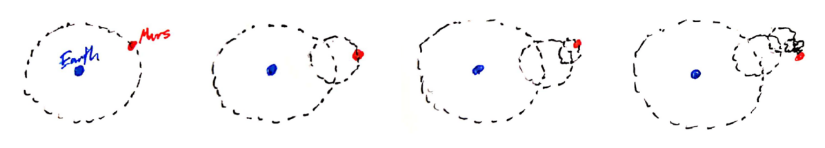
Figure 1: Schematic progression of epicycles needed in the Ptolemaic model of Mars orbiting the Earth as astronomical measurements increased in precision.

So why did sixteenth century physicists favor Kepler’s laws and heliocentrism? The discriminating factor is manifestly not which model better-fitted the data. Rather, the choice comes down to Occam’s razor, to explanatory power, to simplicity and to fine-tuning of parameters. Physicists favor theories which do more with less—theories which explain more about the world while requiring fewer inputs. This is a subjective bias about how we think the universe should work, and it’s possible that this philosophy will ultimately fail—but it’s been working well thus far.

While keeping the above intuition firmly in the back of our minds, it can be useful to introduce a mathematical classification of this fine-tuning, with the understanding that no such measure is god-given and so what to do with such a measure is up to us. We’ll discuss a couple such schemes, the first being a mathematical formalization of the dependence of an output of interest on the values of the inputs. This has the benefit that it is intuitive and simple to compute, so it is widely used in the particle physics literature. However, it lacks independence under how variables are parametrized so can lead to misleading conclusions if used without care.

Furthermore, it will assign a measure of fine-tuning to individual points in the parameter space of a model, whereas we’d like to characterize the naturalness of a model as a whole—if a model only produces predictions that match the real world in a small region of its parameter space, that’s another important element of fine-tuning [93]. For example, if new data removes all but a small fraction of the viable parameter space in a given model, we want to regard that model as being less natural afterward. An approach based on Bayesian statistics allows us to incorporate these issues and gives unambiguous comparisons of the relative naturalness of models upon the collection of new data [94], but loses out on simplicity.

A simple and often-used measure was introduced by Giudice and Barbieri [95], who suggested the definition

$$\Delta_{X}\equiv\left|\frac{\text{d}\ln m^{2}}{\text{d}\ln X}\right|=\left|\frac{X}{m^{2}}\frac{\text{d}m^{2}}{\text{d}X}\right|$$ (3)

which may be called a measure of the fine-tuning of the input parameter $X$ necessary to get out the correct output parameter $m^{2}$. The logarithmic dependence naturally gives a measure of relative sensitivity and removes dependence on overall scale or choice of units. If $\Delta_{X}$ is large, this denotes a large sensitivity of $m^{2}$ to the value of $X$, and implies that one must choose the value of $X$ very carefully to get out the right physics. In the example in Equation 2 above we have $\Delta_{\lambda}=\frac{\lambda}{m_{\phi}^{2}}\nu^{2}\simeq\frac{M^{2}}{m_{\phi}^{2}}\simeq 10^{28}$, indeed signaling enormous fine-tuning, and likewise $\Delta_{\nu^{2}}=\lambda\frac{\nu^{2}}{m_{\phi}^{2}}$. Contrast this with the familiar case of a seesaw mechanism where the light neutrino mass is given by a formula like $m_{\nu}^{2}=m^{4}/M^{2}$, with $M$ a heavy mass scale and $m$ a weak scale mass. We can check whether this mechanism requires fine-tuning with $\Delta_{M^{2}}=\frac{M^{2}}{m^{2}_{\nu}}\frac{m^{4}}{M^{4}}=\frac{1}{m_{\nu}^{2}}\frac{m^{4}}{M^{2}}=1$, and we find that seesaw mechanisms are natural. So $\Delta_{X}$ matches our intuition here, and can be quite useful.

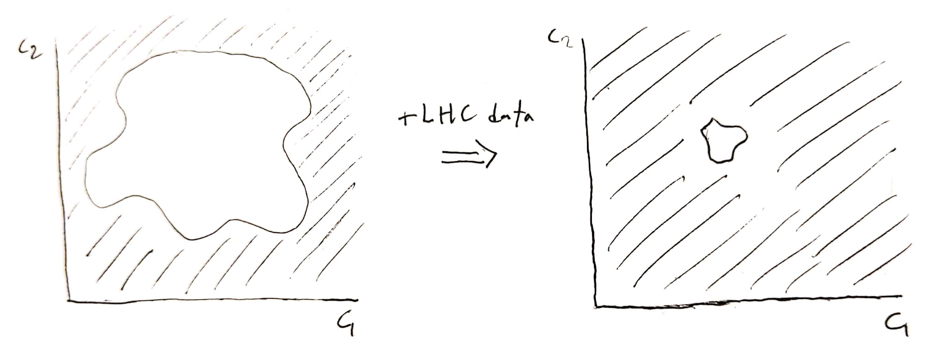
Figure 2: A schematic representation of the LHC ruling out previously-viable parameter space in some model. Surely afterwards we should view this model as more fine-tuned compared to a model on which the LHC results had no impact.

However, for a model with free parameters a notion of fine-tuning at a single point in parameter space does not capture the full picture, and we should incorporate a notion of the volume of viable parameter space into our naturalness criterion [96], as diagrammed in Figure 2. This necessity should be intuitive in the context of constraining models of new physics. Models which achieve their aim throughout parameter space are viewed more favorably than models which only work in some small region of their parameter space. For a relevant example, there are still corners of the MSSM parameter space that are natural under the Giudice-Barbieri measure. But the fact that the LHC has ruled out large swathes of this parameter space means that we should surely view weak-scale supersymmetry as less natural now than we did a decade ago. A pointwise measure of fine-tuning misses this.

An approach based on Bayesian statistics can be used to better match what we want from a measure of naturalness, as is discussed well in [84]. The definition of a model in a Bayesian framework requires priors on its free parameters $\{\theta_{i}\}$, denoted $p(\theta_{i}|\mathcal{M})$, and different choices of $\{p(\theta_{i}|\mathcal{M})\}$ should be considered different models. The probabilist’s notation $p(A|B)$ may be interpreted as ‘the probability of $A$ given that $B$ is true’. We also require a prior probability $p(\mathcal{M})$ that the model $\mathcal{M}$ is true as a whole. After we receive data $d$, Bayes’ theorem gives us the posterior probability for the model as

$$p(\mathcal{M}|d)=\frac{p(d|\mathcal{M})p(\mathcal{M})}{p(d)}$$ (4)

where $p(d|\mathcal{M})$ is known as the likelihood. Both $p(\mathcal{M})$ and $p(d)$ are explicitly subjective, but if we take the ratio of the posterior probabilities for two models $\mathcal{M}_{1}$ and $\mathcal{M}_{2}$ we find

$$\frac{p(\mathcal{M}_{1}|d)}{p(\mathcal{M}_{2}|d)}=\frac{p(d|\mathcal{M}_{1})}{p(d|\mathcal{M}_{2})}\frac{p(\mathcal{M}_{1})}{p(\mathcal{M}_{2})}$$ (5)

This expresses how the ratio of the likelihood of these two models changes after receiving new data. So while different physicists may disagree on the prior and posterior probabilities, the ‘Bayes update factor’ $B\equiv p(d|\mathcal{M}_{1})/p(d|\mathcal{M}_{2})$ is unambiguous and shows that the physicists agree on how the relative naturalness of the two models is affected by the new data.

The likelihood in a model with free parameters $\{\theta_{i}\}$ is calculated as

$$p(d|\mathcal{M})=\int\left(\prod_{i}d\theta_{i}\right)p(d|\mathcal{M},\theta_{i})p(\theta_{i}|\mathcal{M})$$ (6)

This is an integration over parameter space of the likelihood of producing the data in this model, weighted by the prior probability distribution we’ve placed on our parameters. This balances the competing effects of how well parameter points fit the data with the principle of parsimony—models with large regions of parameter space which don’t fit the data are penalized. The need to compare models to define naturalness in a Bayesian formalism is easily seen by the fact that the likelihood for any new physics model decreases monotonically as more data is collected and previously-viable regions of parameter space are ruled out (in the absence of a discovery, of course).

An interesting playground for these ideas is the strong CP problem. In brief, this is the smallness of the so-called ‘theta angle’ $\theta$ in QCD, which controls the amount of CP breaking in the strong sector. While $\theta\in\left[0,2\pi\right)$, empirical measurements now constrain $\theta\lesssim 10^{-10}$. Although $\theta$ is not technically natural, in the Standard Model it runs very slowly—since the other source of CP breaking is from the CKM matrix—such that if one sets it tiny in the UV, it stays small down to the IR. The Guidice-Barbieri measure would thus produce $\Delta_{\theta_{\text{UV}}}\simeq 1$, as the measured value is insensitive to small changes in the UV value. And yet, the small theta angle is regarded as a naturalness problem, which can be justified in a Bayesian approach. The necessity of a prior does help quantify one’s surprise at the small value of $\theta$ in the context of the Standard Model, but to really think about naturalness we need to have a comparison. We know of simple theories which produce vanishing $\theta$ starting from generic values of the parameters—for example, an axion naturally produces $\theta=0$. Then if we have new data which pushes down the upper bound on $\theta$, axion models receive large Bayesian update factors in relation to the Standard Model. When we know of a simple model which automatically explains some data, it’s puzzling if our current model requires precise choices for free parameters in order to explain the data.

We can see these notions play out for the hierarchy problem by comparing our toy model of a GUT to one with weak-scale supersymmetry. Our toy model in Section 1 produced a scalar through a cancellation of GUT-scale $\sim 10^{16}\text{ GeV}$ contributions. A toy model with supersymmetry (to be discussed in Section 1) would remove sensitivity to the ultraviolet, and replace the scale of GUT-breaking with the effective scale of supersymmetry-breaking in the SM sector $\tilde{m}$. And while the GUT scale is (more or less) fixed by the running of SM couplings, the SUSY-breaking scale in the SM can be far lower. We use $\tilde{m}$ here as a one-parameter avatar of the scale of superpartners. The general prediction for supersymmetry before the LHC was $\tilde{m}\sim\mathcal{O}(100\text{ GeV})$, with multiple species of superpartners appearing below the TeV scale. Such a model produces an improvement in Giudice-Barbieri tuning of $\delta\Delta\sim 10^{28}$ over our model without SUSY.

Let’s take $p(\tilde{m}|\text{weak scale SUSY})$ to be a logarithmic prior from $m_{\text{low}}$ to $m_{\text{high}}$, where an upper limit $m_{\text{high}}\sim 500\text{ GeV}-1\text{ TeV}$ is justified by the requirement that the model give small Higgs mass corrections and a weak-scale dark matter candidate. If we collect collider data for a decade and find that much of the parameter space is ruled out, say with a limit $\tilde{m}\geq\mathfrak{m}$ we should update our thoughts on the naturalness of the model. This data has no effect on our non-SUSY GUT model, as it predicts no new light particles, but there has been a large effect on our SUSY model as its most favored parameter space has been ruled out. So we have a large Bayesian update factor.

$$B \equiv\frac{p(\text{LHC data}|\text{non-SUSY GUT})}{p(\text{LHC data}|\text{weak scale SUSY GUT})}$$ (7)

$$=\frac{1}{\left(\log\frac{m_{\text{high}}}{m_{\text{low}}}\right)^{-1}\int_{\mathfrak{m}}^{m_{\text{high}}}\frac{\text{d}\tilde{m}}{\tilde{m}}}$$

$$=\log\frac{m_{\text{high}}}{m_{\text{low}}}/\log\frac{m_{\text{high}}}{\mathfrak{m}}$$

Of course supersymmetric extensions of the SM have a large number of parameters, and how to translate to an upper bound $\mathfrak{m}$ on our one-parameter version isn’t well-defined, but certainly much of the previously-favored parameter space has been ruled out. The general lesson is that models which don’t predict new visible states near the weak scale have received large Bayesian update factors from the LHC. This doesn’t give a strict mandate for our overall relative belief, as one may argue there are good reasons to take a large prior for supersymmetry and expect always to find superpartners right around the corner. After all, even if $\tilde{m}\sim 1000\text{ TeV}$, it would still have $\delta\Delta\sim 10^{20}$ Giudice-Barbieri tuning better than the GUT without SUSY. But it does motivate further investigation of models which don’t succumb to this issue, be they neutral naturalness modules which push the scale of new visible states up by a loop factor or more radical ideas about the origin of the electroweak scale.

Furthermore, we can directly input physics into making a sensible choice of the prior one places on a model, and there has been much discussion of justifying simple choices. The dictum of Dirac naturalness mandates priors peaked at $\mathcal{O}(1)$ values. But with a model which makes some parameter technically natural one, a prior that allows small values is justified, such as a logarithmic prior. An explicit example of this modification of priors by physics can be seen in the application of the Weak Gravity Conjecture to the hierarchy problem [97, 98, 99, 100, 101, 102, 103, 104, 11, 5, 105], which will be discussed in more detail in Section 1. This mechanism explicitly modifies the prior one should have on UV theories by linking the notion of the Swampland—that some string vacua don’t admit universes like ours—to the allowed range of Higgs masses. This addresses the hierarchy problem by constructing a model where the priors are forced by UV physics to favor a light Higgs.

While these measures of naturalness are useful to help us clarify our expectations, we emphasize again that they must be used sensibly. But it’s clear that some notion of naturalness appears solely from the axioms of probability, and is indeed baked-in to the practice of science inquiry. That’s not to say that we should be epistemologically committed to the naturalness of the universe, but we can still see it as a useful guide toward new physics which has worked well in the past.

3 The Lonely Higgs

All models are wrong, but some are useful.

George E. P. Box
Robustness in the Strategy of
Scientific Model Building (1979) [106]

There is another obvious suggestion that is useful to discuss: perhaps the Higgs does not interact with any physics at higher mass scales, such that despite in principle worries about the hierarchy problem there is no hierarchy problem in practice. The physics which can destabilize the Higgs mass must, as seen in the above example, both be heavier than the Higgs and interact with it in order to generate a contribution. Since the Higgs mass in the SM is not technically natural (that is, it is UV sensitive), large mass corrections from such particles are generic, as we saw in Section 3. One can explore the idea that perhaps there are no such particles. This faces a number of challenges.

The first difficulty is that we know there must be new physics. The Standard Model does not explain neutrino masses nor dark matter, though it is possible that both of these be resolved without introducing new heavy particles. But a deeper issue is that we know the SM cannot be a fundamental theory because the Landau pole in hypercharge makes it inconsistent. This demands that something must happen to rid the theory of this pole, and it will interact with the Higgs because the Higgs is hypercharged. This is one motivation for thinking that something like Grand Unification must take place, and of course its breaking introduces a heavy fundamental scale. One can try to get around this by appealing to quantum gravity coming in at scales below that of the Landau pole. But the Higgs certainly interacts gravitationally, so for this program to succeed one needs a quantum gravitational theory which does not introduce any scales. This is interesting to explore, but does not seem to be the way the universe works, though we leave detailed criticism of this idea to the gravity theorists.

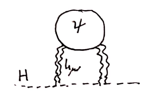
(a)

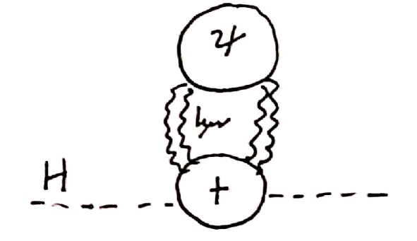
(b)

Figure 3: In (a), a representative two-loop diagram giving gravitational corrections to the Higgs mass from a new dark fermion $\psi$. These diagrams do not destabilize the Higgs mass. In (b), a representative three-loop diagram in which the gravitons couple to an off-shell top quark, which is no longer proportional to the Higgs mass.

Furthermore, even if somehow all heavy particles are neutral under the SM gauge groups, there is no way for them to escape gravitational interactions with the Higgs. This leads to irreducible three-loop corrections to the Higgs mass [107], as depicted in Figure 3. Consider a fermion $\psi$ with mass $M_{\psi}$. The obvious two-loop diagram where the graviton couples to the Higgs directly gives a correction proportional to $m_{H}^{2}$, as the graviton coupling to a massless on-shell particle vanishes at zero momentum. However, we can draw a diagram where a $\psi$ loop talks gravitationally to an off-shell top loop contribution to the Higgs two-point function, and integrating this particle out yields a correction

$$\delta m_{H}^{2}\simeq\frac{y_{t}^{2}}{(16\pi^{2})^{3}}\frac{M_{\psi}^{4}}{M_{pl}^{4}}M_{\psi}^{2}+\text{ subleading}.$$ (8)

The powers of $M_{\psi}$ appear because the only other possible mass scale for the numerator is $m_{t}=y_{t}v$, and the top loop power-law correction to the Higgs mass does not vanish in the $v\rightarrow 0$ limit. The sensitivity of the Higgs mass is softened by three loop factors as well as by the Planck mass from the gravitational couplings, but insisting that $\delta m_{H}^{2}\lesssim(1\text{ TeV})^{2}$ places an upper ‘naturalness’ limit on such fermions of $\sim 10^{14}\text{ GeV}$. While far better than the $\sim 1\text{ TeV}$ limit for SM-charged particles, this is still well below the Planck scale and amounts to an enourmous constraint on UV physics. In fact the problem is a bit worse than this estimate, as we should sum over all SM loops that couple to the Higgs, but this suffices already to see the issue.

So asking for the Higgs to be lonely enough to cure the hierarchy problem is a humongous requirement on the ultraviolet of the universe, and this approach faces a number of important hurdles. We mention that there is work on interesting theories which touch on some of these points, but as a whole Nature seems not to have taken this approach.

4 Mass-Independent Regulators

One may hear the statement that the hierarchy problem disappears if you use a mass-independent regularization scheme, for example dimensional regularization. Unlike the prior nonsolutions we’ve considered, this one is definitively incorrect. The mass scale one introduces in EFT is a stand-in for genuine physical effects of any sort which appear at shorter distance scales. So the cutoff regularization is useful for seeing an avatar of the hierarchy problem even when one does not know the ultraviolet theory. With a mass-independent scheme, one must instead put in specific short-distance physics to see the problem, but we can easily see the general issue.

As a simple example, take a theory with two real scalars - our light $\phi$ and a heavier $\varphi$. If we impose a $\mathbb{Z}_{2}$ symmetry for simplicity, the action is

$$S=\int d^{4}x\left[-\frac{1}{2}(\partial_{\mu}\phi)^{2}-\frac{1}{2}m_{0}^{2}\phi^{2}-\frac{1}{2}M_{0}^{2}\varphi^{2}-\frac{\lambda}{4}\phi^{2}\varphi^{2}\right]$$ (9)

Doing continuum effective field theory with dimensional regularization and the $\overline{\text{MS}}$ renormalization scheme, we must upgrade the masses and couplings to running parameters which depend on the renormalization scale $\mu$, as usual (introduced in Section 2). Since our renormalization scheme is mass-independent, if we want to study physics at an energy scale $\mu\sim m_{\phi}\ll M_{\varphi}$, we should implement the decoupling theorem by hand. We integrate out the heavy degree of freedom at the scale $\mu\sim M_{\varphi}$ and match to a low-energy effective field theory which only contains the low-energy degree of freedom $\phi$ (introduced in Section 3). So let us go ahead and integrate out the heavy scalar $\varphi$. The effect on the $\phi$ mass comes from the simple diagram of Figure 4.

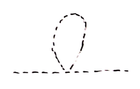
Figure 4: The one-loop diagram for a scalar quartic interaction contributing to a scalar mass.

We go to general dimension $d=4-\epsilon$ and replace $\lambda\rightarrow\lambda\tilde{\mu}^{\epsilon}$, where $\tilde{\mu}$ is an arbitrary scale which soaks up the mass dimension of $\lambda$ away from $d=4$. The resources needed to compute the integrals for general dimension and to take the limit $\epsilon\rightarrow 0$ can be found in Srednicki’s textbook [18].

$$-i\delta m^{2} =\frac{-i\lambda\tilde{\mu}^{\epsilon}}{2}\int\frac{d^{d}k}{(2\pi)^{d}}\frac{-i}{(k^{2}+M_{\varphi}^{2})}$$

$$=\frac{-i\lambda\mu^{\epsilon}}{2}\int\frac{d^{d}\bar{k}}{(2\pi)^{d}}\frac{1}{(\bar{k}^{2}+M_{\varphi}^{2})}$$

$$=-i\frac{\lambda\tilde{\mu}^{\epsilon}}{2(4\pi)^{2}}\Gamma(-1+\frac{\epsilon}{2})(4\pi)^{\frac{\epsilon}{2}}(M_{\varphi}^{2})^{1-\frac{\epsilon}{2}}$$

$$=i\frac{\lambda}{2(4\pi)^{2}}M_{\varphi}^{2}\left[\frac{2}{\epsilon}-\gamma_{E}+1+\ln 4\pi-\ln M_{\varphi}^{2}+2\ln\tilde{\mu}+\mathcal{O}(\epsilon)\right]$$

$$=i\frac{\lambda}{(4\pi)^{2}}M_{\varphi}^{2}\left[\frac{1}{\epsilon}+\frac{1}{2}+\ln\frac{\mu^{2}}{M_{\varphi}^{2}}+\mathcal{O}(\epsilon)\right]$$ (10)

Where $\gamma_{E}$ is the Euler-Mascheroni constant, and we have Wick rotated $k^{0}\rightarrow i\bar{k}^{d}$, integrated in general dimension, expanded in the limit $\epsilon\rightarrow 0$ and defined $\mu^{2}\equiv 4\pi\tilde{\mu}^{2}e^{-\gamma_{E}}$ to soak up the annoying constants. Indeed, we see that there’s no quadratic divergence, which ultimately is due to the fact that scaleless integrals vanish in dimensional regularization $\int\frac{d^{d}k}{k^{n}}=0$, as must be true simply by dimensional analysis.

Now we follow the $\overline{\text{MS}}$ renormalization scheme by adding a counterterm which cancels off the divergent piece and we match at $\mu=M_{\varphi}$ to ensure that our low-energy EFT produces the same predictions as the UV theory, as discussed in Section 3. This gives us

$$S=\int d^{d}x\left[-\frac{1}{2}(\partial_{\mu}\phi)^{2}-\frac{1}{2}\left(m_{0}^{2}+\frac{\lambda}{(4\pi)^{2}}M_{\varphi}^{2}\right)\phi^{2}-\dots\right]$$ (11)

We see that the high-energy degree of freedom $\varphi$ contributes a threshold correction when we flow to lower energies and remove it from the spectrum. While there was never a quadratic divergence, we still found a large quadratic correction to the mass of the scalar $\phi$ which is proportional to the scale of new physics.

This underscores the importance of not getting confused by unphysical features of renormalization. There is a physical issue, which is the sensitivity of the physical low-energy scalar mass to the physics in the ultraviolet. Indeed if we tame the UV in different ways, we find different avatars of this sensitivity. It’s true that a Wilsonian cutoff acts as a stand-in for arbitrary scaleful physics, which is why it’s more direct to see the issue in that picture, but the same physical problem appears regardless of the regularization.

3 The Hierarchy Problem

After discussing those misconceptions, we may give a one-sentence description of the hierarchy problem:

In a theory of physics beyond the Standard Model where the Higgs mass is an output, physical parameters must be finely-tuned in order to produce a mass which is far below the scale of new physics, in tension with the principle of parsimony.

With that in hand, we are prepared to delve in to how the hierarchy problem may be solved in the next section. Our discussion below will not take place within a UV complete extension of the Standard Model, so one might worry that we are attacking a problem without knowing its source. While true, the point from Section 3 is that the sensitivity to UV physics is so general that we expect to need a mechanism which stabilizes the Higgs mass to whatever new heavy physics is out there. Our toy calculation of the relative naturalness of SUSY already evinces this point—SUSY tamps UV sensitivity no matter what it is, so the details of the UV completion are immaterial. As a result of this idea, we will mostly worry just about finding a way to produce a light scalar and assume that it can be embedded into whatever physics exists at high scales, rather than committing to a particular framework of grand unification or what have you. Of course it’s possible that interesting mechanisms to produce an IR scale do rely on particular properties of the UV, and we’ll discuss this important idea in Section 3. But even there, our initial goal is simply to produce a light scalar which is compatible with the Standard Model, rather than to write down a full theory of the universe on all scales. If we can first solve the problem in a toy model which shares some features of our universe, then we can hope to abstract what we learn from that to solve the real problem.

Chapter 2 The Classic Strategies

Without going out of my door
I can know all things on earth
Without looking out of my window
I could know the ways of heaven

George Harrison satirizing the
past decades of particle theory
in light of LHC data
The Inner Light (1968) [108]

Fantastic Symmetries and How To Break Them

In large part the story of particle physics over the past decades is the story of attempts to solve the hierarchy problem. Much theoretical effort has been put into understanding interesting symmetries and mechanisms for breaking them, and more generally ways that small numbers can pop out of physical theories; and much experimental effort has focused on locating empirical hints of these ideas. However, the past few years have seen many practitioners turn their attention toward topics like dark matter, cosmology, and astrophysics. And for good reason—on the experimental side, this is largely where the new data is and will be for the foreseeable future, and at the purely theoretical level the hierarchy problem has become a lot more challenging, as we will argue below. But this has lead to a new generation of particle theorists who are largely unfamiliar with the fantastic and brilliant ideas which drove the field in the prior couple decades.

Despite the fact that we will argue below that these ideas largely appear to not be the way the world works at the weak scale, understanding this prior work can be enormously helpful for inventing novel ideas in the future. It is with this in mind that we introduce below the basics of a variety of interesting ideas and methods in particle physics against the backdrop of their relevance to the hierarchy problem. These are ideas that have not yet made their way into standard textbooks on field theory, but are nevertheless essential topics for students of particle theory to absorb. We will endeavor to explicate the core of these ideas in the simplest models possible, and will largely avoid discussing phenomenological considerations past producing a light scalar. The discussion will not be at the level of depth required for research in the field, but will hopefully be a nice overview of interesting topics for which references to serious introductions and reviews will be provided as well.

So how does one solve the hierarchy problem? The classical solutions may be conceptually divided into two steps. First one introduces some structure above the electroweak scale which protects the Higgs mass from large contributions due to UV physics. This could be something like a new symmetry which forbids a scalar mass term, or a modification to spacetime on small length scales, or the dissolution of a non-fundamental Higgs into component fields.

However, the Higgs is not exactly massless, which is due to the fact that whatever structure we add is not a feature of the low-energy Standard Model. There must thus be some IR dynamics that break that UV structure at the electroweak scale to ensure that we end up with the Standard Model at low energies. Depending on the UV structure this may be something like spontaneous symmetry breaking or moduli stabilization or dimensional transmutation.

There are two big categories of classical solutions. One is to find a field-theoretic mechanism which prevents contributions to the Higgs mass in the UV. Supersymmetry is the prime example here. The other is to bring the fundamental cutoff of the theory down to the infrared, such that in the UV there’s no Higgs to talk about. This is exemplified by composite Higgs theories or theories where the cutoff of quantum gravity is lowered to the weak scale.

To evince these strategies, we’ll go through a couple examples of ways to forbid scalar masses and to break those structures. Our aim here is not to construct realistic theories of the Higgs but rather to understand these general principles, so we’ll study simple toy models which allow us to appreciate the essential points.

1 Supersymmetry

Superpartners aren’t essential
But would have been consequential
Such wasted superpotential
Super once, super twice
Super chicken soup with rice

Maurice Sendak on his disappointment with the LHC data
Lost Stanza of Chicken Soup with Rice (1962) [109]

Supersymmetry exploits a loophole in the classic Coleman-Mandula theorem [74] by introducing fermionic symmetry generators, which in layman’s terms turn bosons into fermions and vice-versa. By the Haag–Łopuszański–Sohnius theorem [110], this is the unique extension to the Poincaré algebra. Since we know that symmetries tend to make physics easier, it is not surprising that supersymmetry is an indispensable tool in high energy theory, regardless of how or whether it is realized in the real world. Some useful general introductions to supersymmetry in $d=4$ and its application to the real world are Terning’s book [111], Martin’s periodically-updated lecture notes [112], and Shih’s video lectures [113], in roughly increasing order of friendliness to neophytes.

In a supersymmetric theory fields come in multiplets which include particles of different spins (so called ‘supermultiplets’) all having the same mass and quantum numbers. We add fermionic generators $Q_{\alpha}$ and $Q^{\dagger}_{\dot{\alpha}}$, called supercharges, with the defining (anti)commutation relations

$$\left\{Q_{\alpha},Q^{\dagger}_{\dot{\alpha}}\right\}=2\sigma^{\mu}_{\alpha\dot{\alpha}}P_{\mu}\quad\left\{Q_{\alpha},Q_{\beta}\right\}=0=\left\{Q^{\dagger}_{\dot{\beta}},Q^{\dagger}_{\dot{\alpha}}\right\}$$ (1)

$$\left[Q_{\alpha},P_{\mu}\right]=0=\left[P_{\mu},Q^{\dagger}_{\dot{\alpha}}\right]$$ (2)

where $P_{\mu}$ is the generator of spacetime translations and $\sigma^{\mu}=(1,\vec{\sigma^{i}})$ with $\sigma^{i}$ the Pauli matrices. These may be determined simply by writing down all objects with the correct index structure. For later use, recall that spinor indices are raised/lowered with the invariant antisymmetric symbols $\epsilon_{\alpha\beta},\epsilon_{\dot{\alpha}\dot{\beta}}$, as used for example in defining the conjugate invariants $(\overline{\sigma}^{\mu})^{\dot{\alpha}\alpha}\equiv\sigma^{\mu}_{\beta\dot{\beta}}\epsilon^{\alpha\beta}\epsilon^{\dot{\alpha}\dot{\beta}}$.

We want to find irreducible representations of the supersymmetry algebra, called supermultiplets. Since $P_{\mu}P^{\mu}=m^{2}$ commutes with the generators $Q_{\alpha}$, $Q^{\dagger}_{\dot{\alpha}}$, the different particles in a supermultiplet will have the same mass. As an example of how to generate supermultiplet states, consider a massive particle. We can go to its rest frame, where it has momentum $P_{\mu}=(m,0,0,0)$ with $m$ its mass. Then the supersymmetry algebra greatly simplifies to $\left\{Q_{\alpha},Q^{\dagger}_{\dot{\alpha}}\right\}=2m\mathds{1}_{\alpha\dot{\alpha}}$, and we see that this is just a Clifford algebra of raising and lowering operators. We define a lowest weight state, or Clifford vacuum $\ket{\Omega_{s}}$ such that it is annihilated by the undotted generators

$$\ket{\Omega_{s}}=Q_{1}Q_{2}\ket{m,s,s_{z}}$$ (3)

$$\Rightarrow Q_{1}\ket{\Omega_{s}}=0=Q_{2}\ket{\Omega_{s}}$$ (4)

Now we can use the dotted generators as raising operators to generate the entire multiplet.

$$\ket{\Omega_{s}}$$ (5)

$$Q^{\dagger}_{\dot{1}}\ket{\Omega_{s}},Q^{\dagger}_{\dot{2}}\ket{\Omega_{s}}$$ (6)

$$Q^{\dagger}_{\dot{1}}Q^{\dagger}_{\dot{2}}\ket{\Omega_{s}}$$ (7)

A single fermionic supersymmetry generator must change the spin of a state by $\frac{1}{2}$. Starting at the top with a spin $j$ particle gives us states of spin $j-\frac{1}{2}$ and $j+\frac{1}{2}$ on the middle line, and another state of spin $j$ on the bottom line. In $d=4$ the supermultiplet formed from a vacuum state of spin $\frac{1}{2}$ is called a ‘vector multiplet’ and contains four states with spins $(0,\frac{1}{2},\frac{1}{2},1)$. That formed from spin 0 is called a ‘chiral multiplet’, and has states with spins $(0,0,\frac{1}{2})$. Note that this is fewer degrees of freedom, since negative spins are not allowed. Beginning with spins higher than $\frac{1}{2}$ leads to states with spins greater than $1$, which will take us into supergravity and will not be necessary for our purposes.

We could repeat this exercise for massless supermultiplets, labelling states by their energy and helicity $\ket{E,\lambda}$. We would find a Clifford algebra with only one set of raising/lowering operators, and find supermultiplets with helicities $\lambda$ and $\lambda+\frac{1}{2}$ for some starting $\lambda$. Then CPT invariance would force us to add states of helicity $-\lambda$ and $-\lambda-\frac{1}{2}$.

Merely from the definition of the symmetry group there are already a few interesting immediate results. For a start, we show that physical states have nonnegative energy in a supersymmetric theory, and the vacuum energy is an order parameter for supersymmetry breaking. First, let’s give a simple expression for the Hamiltonian operator of supersymmetry. We act on our anticommutation relation with $(\overline{\sigma}^{\nu})^{\dot{\alpha}\alpha}$ and recall various identities to note that $\sigma^{\mu}_{\alpha\dot{\alpha}}(\overline{\sigma}^{\nu})^{\dot{\alpha}\alpha}=2\eta^{\mu\nu}$, which gives us

$$4P^{\nu}=(\overline{\sigma}^{\nu})^{\dot{\alpha}\alpha}\left\{Q_{\alpha},Q^{\dagger}_{\dot{\alpha}}\right\}$$

$$\Rightarrow 4P^{0}=4H=\mathds{1}^{\dot{\alpha}\alpha}\left\{Q_{\alpha},Q^{\dagger}_{\dot{\alpha}}\right\}$$

$$4H=Q_{1}Q^{\dagger}_{\dot{1}}+Q^{\dagger}_{\dot{1}}Q_{1}+Q_{2}Q^{\dagger}_{\dot{2}}+Q^{\dagger}_{\dot{2}}Q_{2},$$

where we have used the fact that the zeroth component of the generator of spacetime translations is the generator of time translations, which is the Hamiltonian operator. Then we can write the energy of some state state $S$ as

$$\bra{S}H\ket{S}=\frac{1}{4}\left(||Q_{1}\ket{S}||^{2}+||Q^{\dagger}_{\dot{1}}\ket{S}||^{2}+||Q_{2}\ket{S}||^{2}+||Q^{\dagger}_{\dot{2}}\ket{S}||^{2}\right)\geq 0,$$ (8)

so the energy of $S$ is non-negative. Furthermore, consider a vacuum state $\ket{0}$ of our theory. In a standard QFT, the vacuum energy $\bra{0}H\ket{0}=E_{\text{vac}}$ is non-physical—we can just shift the Hamiltonian arbitrarily to remove it. But here, the supersymmetry algebra gives a preferred frame. If a vacuum state $\ket{0}$ is supersymmetric then it is annihilated by the supercharges $Q_{\alpha}\ket{0}=0,Q^{\dagger}_{\dot{\alpha}}\ket{0}=0$, otherwise the vacuum would not be invariant under supersymmetry transforms. This implies that it will have vanishing total energy $\bra{0}H\ket{0}=0$. Conversely, if the vacuum state is non-supersymmetric, then its energy is strictly positive. We say supersymmetry is broken in such a state. Thus the vacuum energy acts as an order parameter for SUSY breaking.

Connected to that fact is that each supermultiplet contains the same number of fermionic and bosonic degrees of freedom. We can see this by defining an operator $F$ which counts the fermion number of a state, so that bosonic states have eigenvalue $1$ under $(-1)^{F}$, and fermionic states have eigenvalue $-1$. Since the SUSY generators interchange bosonic and fermionic states, they must anticommute with $(-1)^{F}$.

Now, for a given supermultiplet consider the states $\ket{a}$ with the same given four-momentum $p_{\mu}$, $p_{0}=E\neq 0$. Since the supercharges commute with $P^{\mu}$, we know that these must form a complete set of states in this subspace $\sum\limits_{a}\ket{a}\bra{a}=1$. Now consider the trace of the weighted energy operator $(-1)^{F}H/4$.

$$\sum\limits_{a}\bra{a}(-1)^{F}H\ket{a} =\sum\limits_{a}\bra{a}(-1)^{F}QQ^{\dagger}\ket{a}+\sum\limits_{a}\bra{a}(-1)^{F}Q^{\dagger}Q\ket{a}$$

$$=\sum\limits_{a}\bra{a}(-1)^{F}QQ^{\dagger}\ket{a}+\sum\limits_{a}\sum\limits_{b}\bra{a}(-1)^{F}Q^{\dagger}\ket{b}\bra{b}Q\ket{a}$$

$$=\sum\limits_{a}\bra{a}(-1)^{F}QQ^{\dagger}\ket{a}+\sum\limits_{b}\bra{b}Q(-1)^{F}Q^{\dagger}\ket{b}$$

$$=\sum\limits_{a}\bra{a}(-1)^{F}QQ^{\dagger}\ket{a}-\sum\limits_{b}\bra{b}(-1)^{F}QQ^{\dagger}\ket{b}$$

$$=0$$ (9)

where we have suppressed the contracted spinorial indices. This implies that the number of bosonic degrees of freedom is the same as the number of fermionic degrees of freedom in our supermultiplet, which we found to be true in the example we considered above.

There is a beautiful formalism of ‘superspace’ which can be used to make supersymmetric theories far more transparent, but introducing this would be too large of a digression for our purposes. We simply want to see the effects of supersymmetry on (in)sensitivity of low-energy physics to the ultraviolet, for which studying a simple theory of chiral superfields will do. The Wess-Zumino model is the simplest such example which is not free, consisting of a single self-interacting chiral supermultiplet, and was historically the first non-trivial four-dimensional theory proved to be supersymmetric.

We may write down the Wess-Zumino Lagrangian as

$$\mathcal{L}=\int\text{d}^{4}x\left(-\partial_{\mu}\phi^{\star}\partial^{\mu}\phi-m^{2}\phi^{\star}\phi-i\psi^{\dagger}\bar{\sigma}^{\mu}\partial_{\mu}\psi-\frac{1}{2}m\psi\psi-\frac{1}{2}y\phi\psi\psi-\frac{1}{2}ym\phi^{2}\phi^{\star}-\frac{1}{4}|y^{2}|\phi\phi\phi^{\star}\phi^{\star}\right),$$ (10)

where for compactness we’ve left off the Hermitian conjugate terms. To avoid introducing certain technical complications we eschew the proof that this is indeed invariant under a supersymmetric transformation and instead evince its UV insensitivity. For fun we’ll compute without assuming the masses are the same $m_{\phi}\neq m_{\psi}$, as can happen in the presence of soft breaking of the symmetry. t is a simple exercise to show that this theory is invariant under the supersymmetry transformations

$$\phi\rightarrow\phi+\epsilon^{\alpha}\psi_{\alpha},\qquad\psi_{\alpha}\rightarrow\psi-i(\sigma^{\mu}\epsilon)_{\alpha}\partial_{\mu}\phi,$$ (11)

where $\epsilon_{\alpha}$ is an anti-commuting Weyl spinor parametrizing an infinitesimal transformation.

Let’s look at the vacuum energy, which we’ll calculate generally but schematically. A quantum harmonic oscillator has ground state energy $\pm\frac{1}{2}\hbar\omega$ for bosonic and fermionic states respectively, with the sign being familiar from the Casimir effect. If we consider a box of side length $V^{1/D}$, the energy of the fields inside it is

$$E_{0}=\sum\limits_{\vec{k}}^{\text{bosons}}\frac{1}{2}\hbar\omega_{\vec{k}}-\sum\limits_{\vec{k}}^{\text{fermions}}\frac{1}{2}\hbar\omega_{\vec{k}},$$ (12)

where $\vec{k}=(k_{1},k_{2},\dots,k_{D})(2\pi/V^{1/D})$, $k_{i}\in\mathbb{Z}$. Now in QFT each mode has energy $\omega_{\vec{k}}=\sqrt[\ ]{k^{2}+m^{2}}$, and as we make the box bigger $V^{1/D}\rightarrow\infty$, the sum turns into an integral

$$E_{0}=V\int\limits\frac{d^{D}k}{(2\pi)^{D}}\left(\frac{1}{2}\sqrt[\ ]{k^{2}+m_{B}^{2}}-\frac{1}{2}\sqrt[\ ]{k^{2}+m_{F}^{2}}\right),$$ (13)

with $m_{B}$ a boson mass and $m_{F}$ a fermion mass, where the sum over species is implicit. We also recognize $E_{0}/V$ as the vacuum energy density, denoted $\Lambda$, which we can write as

$$\Lambda\simeq\frac{1}{2(2\pi)^{D}}\int\limits d^{D}k\left(\sqrt[\ ]{k^{2}+m_{B}^{2}}-\sqrt[\ ]{k^{2}+m_{F}^{2}}\right).$$ (14)

Now if we specialize to $D=4$ and introduce a cutoff $k_{max}$ up to which we’re confident that our description of particle physics holds, the schematic form is simply

$$\Lambda\sim k_{max}^{4}\left(\sum\limits^{\text{bosons}}1-\sum\limits^{\text{fermions}}1\right)+k_{max}^{2}\left(\sum\limits^{\text{bosons}}m_{B}^{2}-\sum\limits^{\text{fermions}}m_{F}^{2}\right)+\dots$$ (15)

Now we see quite generally and explicitly that in a supersymmetric state the vacuum energy vanishes, since there are equal numbers of bosonic and fermionic fields with degenerate masses. Furthermore, spontaneous breaking of supersymmetry breaks the degeneracy but does not change the numbers of fields, so softly broken supersymmetry retains protection from the largest contribution.

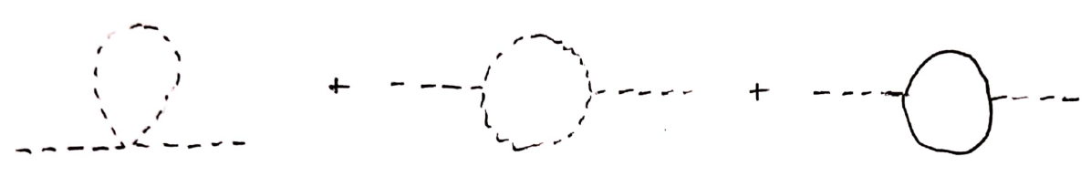
Figure 1: The one-loop diagrams contributing to the scalar mass correction in the Wess-Zumino model.

Let’s look now more sharply at the one-loop contributions to the scalar mass in the Wess-Zumino model, regularized with a hard cutoff $\Lambda$. Take care that we’ve written the Lagrangian in terms of two-component spinors, an exhaustive guide to which can be found in [119]. The three diagrams are shown in Figure 1, and their evaluation proceeds as

$$-i\delta m^{2} =(-im_{\psi}y)^{2}\int\frac{d^{4}k}{(2\pi)^{4}}\frac{(-i)^{2}}{(k^{2}+m_{\phi}^{2})^{2}}+(-iy^{2})\int\frac{d^{4}k}{(2\pi)^{4}}\frac{(-i)}{(k^{2}+m_{\phi}^{2})}$$

$$+(-1)\frac{1}{2}(-iy)^{2}\int\frac{d^{4}k}{(2\pi)^{4}}\frac{(-i)^{2}\text{Tr}\left[\sigma^{\mu}k_{\mu}\bar{\sigma}^{\nu}k_{\nu}\right]}{(k^{2}+m_{\psi}^{2})^{2}}$$ (16)

$$=i|y|^{2}\int\frac{d^{4}\bar{k}}{(2\pi)^{4}}\left[\frac{m_{\psi}^{2}}{(\bar{k}^{2}+m_{\phi}^{2})^{2}}-\frac{1}{(\bar{k}^{2}+m_{\phi}^{2})}+\frac{\bar{k}^{2}}{(\bar{k}^{2}+m_{\psi}^{2})^{2}}\right]$$ (17)

$$=i\frac{|y|^{2}}{16\pi^{2}}\int_{0}^{\Lambda}d\bar{k}\ \bar{k}^{3}\left[\frac{m_{\psi}^{2}-m_{\phi}^{2}-\bar{k}^{2}}{(\bar{k}^{2}+m_{\phi}^{2})^{2}}+\frac{\bar{k}^{2}}{(\bar{k}^{2}+m_{\psi}^{2})^{2}}\right]$$ (18)

$$=i\frac{|y|^{2}}{16\pi^{2}}(m_{\phi}^{2}-m_{\psi}^{2})\log\Lambda+\text{ finite}.$$ (19)

We see that the UV sensitivity of the scalar mass in this theory has disappeared, even if the two fields have different masses. In the limit of unbroken supersymmetry, the contribution vanishes identically.

This fact of removing the UV sensitivity of the mass of a scalar persists generally, no matter which other superfields are added, so long as supersymmetry is at most softly broken. The connection to the hierarchy problem is clear: If, in the UV, all fields come in supermultiplets, then the Higgs mass is protected from UV contributions.

Of course we do not observe mass-degenerate superpartners, so this soft supersymmetry breaking is a necessary feature of any implementation of supersymmetry to the real world. The Minimal Supersymmetric Standard Model [120] embeds each of our fermions in a chiral supermultiplet and each gauge boson in a vector multiplet. The Higgs sector must be enlarged to two chiral multiplets containing the up and down Yukawas respectively, as is necessary for anomaly cancellation.

The question of supersymmetry-breaking is a very non-trivial one. At the level of a phenomenological accounting of possible soft breaking terms in the MSSM, there are 105 physical parameters [122]. However, constraints on flavor-violating couplings and on CP violation tell us empirically that the soft terms that appear must be very non-generic. In fact, looking at the MSSM in detail it turns out there are no places for supersymmetry-breaking to enter directly, and indeed there are general arguments that such breaking must take place in another, hidden sector and be indirectly communicated to the MSSM fields (see e.g. Martin’s Section 7.4 [112]).

The origins of supersymmetry-breaking being a separate sector does force us to expand our model of particle physics, but on the upshot this sequestering means we can explore interesting phenomenology in sectors which are unconstrained. One can write down models where supersymmetry breaking is mediated by supergravity effects [123, 124, 125, 126, 127, 128, 129], communicated to the SM fields by our gauge bosons from a sector with new, massive SM-charged particles [130, 131, 132, 133, 134, 135], or takes place at a physically separate location in an extra dimension [136, 137, 138, 139, 140, 141, 142, 143, 144, 145], for a few examples. A full discussion of the mechanisms and strategies for models of supersymmetry-breaking is beyond our scope, but we highly recommend Intriligator & Seiberg’s lecture notes [146] as a general reference along with Martin’s notes [112].

Of course we would like this phase transition to originate as spontaneous symmetry breaking, rather than explicitly putting it in by hand, since we want the far UV to be supersymmetric. Such spontaneous breaking requires the generation of a scale, and so it would be great if such a scale were generated dynamically, as in the dimensional transmutation we saw in QCD in Section 3. This would then be a natural mechanism for SUSY breaking. This phenomenological prospect lead to and benefited from a fantastic body of work understanding the details of supersymmetric gauge theories e.g. [147, 148, 149, 150, 151, 152, 153, 154, 155, 156, 157], which can be found reviewed in textbooks by Terning [111] and Shifman [158] and in TASI notes by Strassler [159].

We stated above that fields in a given supermultiplet share all the same quantum numbers, but there is in fact one exception. The supersymmetry algebra in Equation 1 is invariant under opposite rephasings of the supercharges $Q_{\alpha}\rightarrow Q_{\alpha}e^{-i\alpha}$, $Q^{\dagger}_{\dot{\alpha}}\rightarrow Q^{\dagger}_{\dot{\alpha}}e^{i\alpha}$. So there is a generator of a global internal symmetry that we may add that has nontrivial commutation relations with the supercharges:

$$\left[R,Q\right]=-Q,\qquad\left[R,Q^{\dagger}\right]=Q^{\dagger}.$$ (20)

This generator is known as an $R$-symmetry generator, and if the theory is invariant under an $R$-symmetry that means that each supermultiplet $\Phi$ can be assigned an $R$-charge $r_{\Phi}$ and the theory is invariant under transformations of each multiplet $\Phi\rightarrow\Phi e^{ir_{\Phi}\alpha}$, schematically, where $\Phi$ is the collection of fields in that multiplet. Since $R$ does not commute with the supercharges, the different fields in the supermultiplet have different $R$-charges. For example if $\Phi$ is a chiral superfield consisting of $(\phi,\psi)$ then under a global rotation by $\alpha$ they transform as

$$\phi\rightarrow\phi e^{ir_{\Phi}\alpha},\qquad\psi\rightarrow\psi e^{i(r_{\Phi}-1)\alpha},$$ (21)

which is simply because $\ket{\psi}\sim Q\ket{\phi}$.

It’s important to emphasize that this $R$-symmetry is not part of the supersymmetry algebra, so one may have supersymmetric theories which do or do not implement $R$-symmetry. Nelson & Seiberg showed a fascinating connection between $R$-symmetry and supersymmetry-breaking [160]. They show roughly that for a low-energy Wess-Zumino model (possibly after having integrated out confined strong dynamics) as long as one has a ‘generic’ potential (in the sense that a generic set of $n$ equations in $n$ unknowns has a solution), then a vacuum spontaneously breaks supersymmetry if and only if it spontaneously breaks $R$-symmetry. The reasoning is simply that such a symmetry imposes an additional constraint on the potential minimization equations, leading to a solution no longer being generically present.

For later use we mention the possibility of ‘extended supersymmetry’, where additional supercharges are added

$$\left\{Q^{A}_{\alpha},Q^{\dagger B}_{\dot{\alpha}}\right\}=2\sigma^{\mu}_{\alpha\dot{\alpha}}P_{\mu},\qquad\left\{Q^{A}_{\alpha},Q^{B}_{\beta}\right\}=0=\left\{Q^{\dagger A}_{\dot{\beta}},Q^{\dagger B}_{\dot{\alpha}}\right\}$$ (22)

where $A,B=1..\mathcal{N}$ index the supercharges. The construction of supermultiplets proceeds as before, but there are now more nonvanishing combinations of supercharges to act on the Clifford vacuum, so supermultiplets are enlarged. In four dimensions, the most supersymmetry we can have without gravity is $\mathcal{N}=4$, which contains enough supercharges to relate the helicity $-1$ vector all the way to the helicity $+1$ vector; any more supercharges would necessarily yield particles of spins $3/2,2$. If we are willing to include these degrees of freedom we can only go up to $\mathcal{N}=8$ ‘supergravity’ (SUGRA), as more charges would lead to a theory with fundamental particles of spins $s>2$ which is pathological. The classic references for supergravity are Wess & Bagger [162] and Freedman & Van Proeyen [163]. Ultimately if supersymmetry is a field-theoretic feature of the ultraviolet of our universe we must have SUGRA as well, as it simply results from applying the supercharges to the graviton field, but we won’t discuss SUGRA any further.

When we enlarge our superalgebra we also enlarge the (potential) R-symmetry group—the group of symmetries which do not commute with the supercharges—since we can now shuffle around the supercharges in addition to rephasing them. We’ll revisit this in Section 3 in the context of utilizing non-trivial R-symmetry representations to break supersymmetry.

2 Extra Dimensions

I exist in the hope that these memoirs, in some manner, I know not how, may find their way to the minds of humanity in Some Dimension, and may stir up a race of rebels who shall refuse to be confined to limited Dimensionality.

Edwin Abbott Abbott,
Flatland, 1884 [164]

One of the most important ideas in theoretical physics developed in the latter part of the $20^{\text{th}}$ century is that there may be additional spatial dimensions past the familiar three of our everyday experiences. Theories in which additional spatial dimensions are present were first studied in the context of unifying gravity and electromagnetism, first by Nordström [165] (before General Relativity!) and then by Kaluza [166] and Klein [167]. These ideas saw a resurgence of interest some half-century later with the advent of string theory, and the vision of all features of the universe being fundamentally geometrized. Against that backdrop, it is clearly prudent to consider the interplay of such theories with the puzzle of the hierarchy problem. As we shall see, extra dimensional theories can produce terribly interesting physics, and the possibilities are manifold.

1 Technology: Kaluza-Klein Reduction

To consider the possibility that there are additional microscopic dimensions, we develop a picture of the effects of fundamentally $D$-dimensional fields where $D=4+d$. On our manifold $M=\mathcal{M}_{4}\times K$, where $K$ is compact, we write down an action

$$S=\int_{\mathcal{M}_{4}}\int_{K}\sqrt[\ ]{-\mathbf{g_{(4+d)}}}\mathcal{L}(\bm{\phi},\mathbf{A}^{M},\mathbf{g}^{MN})$$ (23)

where our fields are in irreducible representations of the $D$-dimensional Poincaré algebra, and the Lagrangian manifestly obeys $D$-dimensional Lorentz invariance. We’ll use boldface for $D$-dimensional fields and Latin letters for $D$-dimensional Lorentz indices. However, since $K$ is compact, it places constraints on the mode expansions of our fields. Then when we want to study the effective four-dimensional theory we first need to decompose our fields into irreducible representations of the $4$-dimensional Poincaré algebra. The $D$-dimensional vectors and tensors will become multiplets of $4$-dimensional fields. Then we can explicitly integrate over the compact manifold $K$, which will produce a tower of states.

As an easy, explicit example, take the compact manifold to be the circle $S^{1}$ of length $2\pi R$, and consider a single complex scalar. We start with

$$S_{5}=\int\text{d}^{4}x\int_{0}^{2\pi R}\text{d}y\left[-\frac{1}{2}\partial_{M}\bm{\phi}^{*}\partial^{M}\bm{\phi}-\frac{1}{2}m^{2}\bm{\phi}^{*}\bm{\phi}\right]$$ (24)

From introductory quantum mechanics, we know that the boundary conditions of being single-valued around the circle constrains the mode expansion of $\bm{\phi}$. We can write

$$\bm{\phi}(x^{\mu},y)=\frac{1}{\sqrt[\ ]{2\pi R}}\sum\limits_{n=-\infty}^{+\infty}\phi_{n}(x^{\mu})e^{iny/R}$$ (25)

where the normalization will produce canonically normalized kinetic terms in the $4$-dimensional action, and should generally be $\sqrt[\ ]{\text{Vol}(K)}$. Plugging this into the action gives

$$S_{5}=\frac{1}{2\pi R}\int\text{d}^{4}x\sum\limits_{mn}\int_{0}^{2\pi R}\left[-\frac{1}{2}\partial^{\mu}\phi^{*}_{m}\partial_{\mu}\phi_{n}-\frac{1}{2}\left(\frac{-im}{R}\right)\left(\frac{in}{R}\right)\phi^{*}_{m}\phi_{n}-\frac{1}{2}m^{2}\phi^{*}_{m}\phi_{n}\right]e^{i(n-m)y/R}$$ (26)

where the first and second terms come from either the $\mathcal{M}_{4}$ derivatives or the $K$ derivatives acting on the mode expansion. The integral over the compact direction now gives, using orthogonality $\int_{0}^{2\pi R}\text{d}ye^{i(n-m)y/R}=2\pi R\delta_{nm}$, a $4$-dimensional action

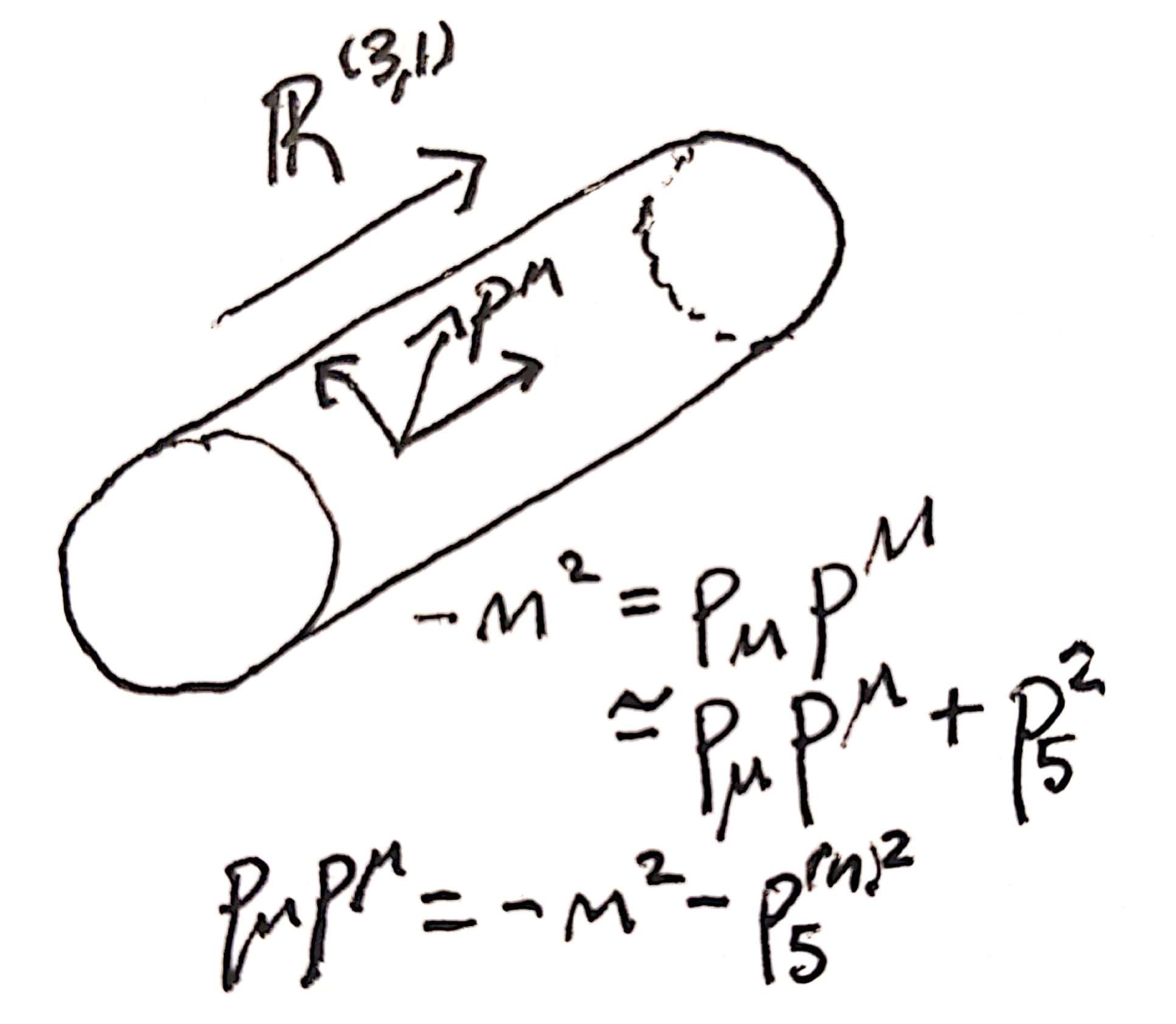
Figure 2: A schematic Kaluza-Klein spacetime for intuition on the appearance of a tower of four-dimensional ‘Kaluza-Klein modes’. The compact extra dimension demands quantized momentum along the fifth dimension. For an observer on large scales, the extra component of momentum appears as a four-dimensional mass term.

$$S_{4}=\int\text{d}^{4}x\sum\limits_{n}\left[-\frac{1}{2}\partial^{\mu}\phi^{*}_{n}\partial_{\mu}\phi_{n}-\frac{1}{2}\left(m^{2}+\frac{n^{2}}{R^{2}}\right)\phi^{*}_{n}\phi_{n}\right]$$ (27)

We see that we now have a tower of $4$-dimensional states that have arisen from the one $5$-dimensional scalar, as shown schematically in Figure 2. There is a ‘zero-mode’ which has a mass given by the $5$-dimensional mass term, and then there are states with larger masses. If $R$ is small, these will be heavy, and so we would only see them at, say, a high energy particle collider. Note that all of these higher levels are doubly-degenerate, since $n$ ranges over all the integers.

If we had included the graviton in this compactification procedure, we would see the $5$-dimensional graviton split up into

$$\mathbf{g}^{MN}=\left(\begin{array}[]{@{}cccc|c@{}}g^{\mu\nu}&&\cdots&&g^{\mu 4}\\ &&&&\\ \vdots&&\ddots&&\vdots\\ &&&&\\ \hline\cr g^{4\nu}&&\cdots&&g^{44}\end{array}\right)$$

so we see the emergence of a $4$-dimensional scalar, vector, and two-index symmetric tensor. And it was in this context that compactification was originally studied as a unification of general relativity and electromagnetism.

There’s another very important effect of the compactification. Let’s consider the Einstein Hilbert action

$$S=\frac{1}{16\pi G_{N}^{(4+d)}}\int_{\mathcal{M}_{4}\times K}R\sqrt[\ ]{-\mathbf{g^{(4+d)}}}\text{d}^{d}x$$ (28)

Noting that the Ricci scalar $R\sim\partial^{2}$ always has mass dimension $\left[R\right]=2$, we see that the $(4+d)$-dimensional Newton’s constant must have $\left[G_{N}^{(4+d)}\right]=2-D=-2-d$, so to rewrite the action in natural units we must define a $(4+d)$-dimensional Planck mass as $1/G_{N}^{(4+d)}=(M_{pl}^{(4+d)})^{2+d}$. If we take the metric to be independent of the $K$ coordinates, then the integration over $K$ just gives a factor of the volume $V_{K}$ of the compact space

$$S=\frac{(M_{pl}^{(4+d)})^{2+d}}{16\pi}V_{K}\int_{\mathcal{M}_{4}}R\sqrt[\ ]{-g^{(4)}}\text{d}^{4}x$$ (29)

Putting this into the form of the four-dimensional Einstein-Hilbert action, we find $M_{\text{pl}}^{2}=(M_{pl}^{(4+d)})^{2+d}V_{K}$. Taking $V_{K}\simeq R^{d}$ for some radius $R$, we see that if the compact dimensions are not Planck-sized $R\sim 1/M_{\text{pl}}$ but larger for whatever reason, then the effective Planck mass at long distances can be much larger than the fundamental Planck mass.

Now we don’t see zero-mode, different spin partners of our particles which fill out representations of the higher-dimensional symmetry, so this simple compactification cannot be the real way the world is. If we have compact dimensions, they must be such that the symmetry of zero-modes is somehow broken for the SM fields. This is important—we don’t just want to have different $5d$ fields with zero modes or not, we need different four-dimensional components of them to have or not have zero modes. We’ll solve this problem in Section 3.

2 Quantum Gravity at the TeV Scale

In the previous section we noticed that extra dimensions dilute the fundamental Planck mass in the higher-dimensional theory to produce a weaker effective four-dimensional Planck mass. So perhaps we can fix the hierarchy between the electroweak scale and Planck scale by lowering the fundamental scale of quantum gravity. Arkani-Hamed, Dimopoulos, and Dvali proposed that the fundamental Planck scale can be $M_{pl}^{(4+d)}\sim\text{ TeV}$ with the weakness of four-dimensional gravity resulting from the dilution of gravitational flux into the extra $d$ dimensions [168]. Using

$$\left(1\text{ TeV}\right)^{(2+d)/2}\simeq(M_{pl}^{(4+d)})^{(2+d)/2}\simeq M_{pl}^{(4)}/R^{d/2}$$ (30)

where $R$ is the radius of the extra dimensions, we find that a parsimonious $d=3$ spherical dimensions of radius $R\simeq 1\text{ nm}$ suffice to remove the hierarchy problem and accord with Eöt-Wash constraints on the behavior of gravity at scales down to $\sim\mathcal{O}(\mu\text{m})$ [169, 170, 171].

Now a nanometer is tiny compared to human scales, but the associated energy scale is $1/R\simeq 100\text{ eV}$, which is a scale we have quite a bit of information about. In particular, if the Standard Model fields were to propagate in all $4+d$ dimensions then it would be easy to excite the ‘winding modes’ with momentum in the extra dimensions, and we should have observed many finely-space Kaluza-Klein resonances with the same quantum numbers. This is obviously not how the universe works, so to dilute gravity with large extra dimensions one must trap Standard Model fields to the four-dimensional manifold we know and love.

This can be done by imagining we live on a $(3+1)$-dimensional topological defect which is embedded in the larger $(4+d)$-dimensional space. ‘Topological defect’ sounds exotic, but these are just (semi-)familiar non-perturbative objects such as the branes of string theory [172, 173, 174], or the cosmic strings or domain walls that can appear in Higgsed gauge theories and which are introduced well in Shifman’s textbook [158]. The original proposal suggests a weak-scale vortex in which zero-modes of our familiar fields are trapped, which is super cool.

Note that the new physics appearing at the TeV scale in this scenario is about as violent as you could imagine: quantum gravity appears at a TeV! This leads to a variety of fascinating signatures and constraints, even in the absence of concrete model of quantum gravity, though embeddings into string theory have also been found [175, 176, 177]. Very generically there are corrections to the Newtonian gravitational laws [178], all sorts of effects on precision observables [179], a loss of flux of high energy particles into the ambient space either astrophysically [180] or at a collider [144], violations of the global symmetries of the SM since quantum gravity does not respect them [181, 182, 183], and production of Kaluza-Klein gravitons [184] and black holes at TeV-scale colliders [185, 186, 187, 188]. This is a fascinating field which is well worth studying in detail, but unfortunately we do not have the space to do it justice. For more detail we refer to the reviews by Rubakov [189] and Maartens & Koyama [190], and the more introductory notes from Csáki [191], Kribs [192], Pérez-Lorenzana [193], Cheng [194], and Csáki, Hubisz, and Meade [195].

However, shrewd readers will be eager to point out that we haven’t actually solved the hierarchy problem; we’ve merely traded the $m_{H}\ll M_{\text{pl}}$ hierarchy for a $1/R^{(2+d)/2}\ll M_{\text{pl}}^{(4+d)}$ hierarchy. And indeed, it can be difficult to stabilize the size of the extra dimensions in this scheme. But the conceptual leap of considering geometric solutions to the hierarchy problem is incredibly important and leads to many further interesting directions. The next ingredient we need is to control the existence of opposite-spin partners.

3 Technology: Orbifold Reduction

Let us consider a spacetime manifold $M=\mathcal{M}_{4}\times K_{G}$ with $\mathcal{M}_{4}$ four-dimensional Minkowski space and $K_{G}$ a $d$-dimensional compact ‘orbifold’. An orbifold is constructed by ‘modding out’ a manifold $K$ by a discrete symmetry group $G$. A manifold is a space that looks locally like Euclidean space; an orbifold is one which locally looks like the quotient space of Euclidean space quotiented by a finite group. In layman’s terms, quotienting or modding out is just identifying points which are transformed into each other under $G$—our space becomes the space of equivalence classes of $K$ under the action of elements of $G$.

As an illustrative example, consider the line $\mathbb{R}$ and the action of the discrete symmetry $\mathbb{Z}_{2}:x\mapsto-x$. When we form the quotient space and identify points under this $\mathbb{Z}_{2}$ action, we find the half line $\mathbb{R}_{\geq 0}$. You’ll notice that this space has a boundary at $x=0$, which was a fixed point of the symmetry group. Mathematicians would say that the $\mathbb{Z}_{2}$ acts freely except at this point. This is a generic feature, and in fact what makes orbifolds interesting for our purposes. We could have also imagined ‘orbifolding’ $\mathbb{R}$ by the translation $T(2\pi R)$, but this would have produced a compact manifold without boundary, $S^{1}$, because this symmetry has no fixed points. Part of the power of orbifolds comes because the quotient group structure gives us some information about what happens at fixed points - you could imagine just studying the half-line, but it seems natural to consider smooth structures on the manifold and then look at the effects under the identification. This should be evinced later in our examples.

Figure 3: Schematic of the construction of an orbifold from the real line. The real line has a $\mathbb{Z}_{2}(0):x\mapsto-x$ symmetry and a translational $T(2\pi R):x\mapsto x+2\pi R$ symmetry. Modding out by the former yields an orbifold because it has a fixed point, while modding out by the latter returns a regular manifold.

Compactifying on orbifolds also gives us a way to cure our missing partner ills. Consider quotienting the circle by a $\mathbb{Z}_{2}$ which folds the circle over onto itself, $y\simeq 2\pi R-y$. This produces a line segment with boundaries at both ends $y=0,\pi R$. We can alternatively think of this as modding out the real line by both translation and mirroring, producing $\mathbb{R}/T(2\pi R)\times\mathbb{Z}_{2}(0)$. There are then two different sorts of fixed points—$y=0$ is fixed by $\mathbb{Z}_{2}(0)$, and $y=\pi R$ is fixed by $T(2\pi R)\mathbb{Z}_{2}(0)\sim\mathbb{Z}_{2}(\pi R)$. You can then envision this as the circle of length $4\pi R$ with these two discrete identifications, that is $S^{1}(4\pi R)/\mathbb{Z}_{2}(0)\times\mathbb{Z}_{2}(\pi R)$, as depicted in Figure 4.

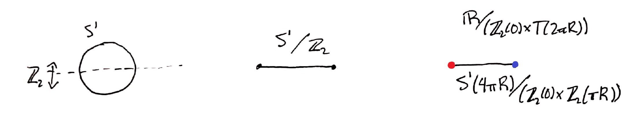
Figure 4: Schematic of the construction of an orbifold from a circle. Quotienting by $\mathbb{Z}_{2}$ corresponds to folding the circle over on itself. We can produce independent fixed points by uplifting first to the real line, or equivalently by folding the circle into quarters.

How does this affect the resulting compactification? As a first step should take our results and rewrite them in terms of eigenfunctions of our $\mathbb{Z}_{2}$ symmetry. We write

$$\bm{\phi}(x^{\mu},y)=\frac{1}{\sqrt[\ ]{\pi R}}\left[\frac{1}{\sqrt[\ ]{2}}\phi_{0}^{(+)}(x^{\mu})+\sum\limits_{n=1}^{+\infty}\phi^{(+)}_{n}(x^{\mu})\cos ny/R+\sum\limits_{n=1}^{+\infty}\phi^{(-)}_{n}(x^{\mu})\sin ny/R\right]$$ (31)

where all we have done is rearrange things by defining

$$\phi^{(+)}_{0}\equiv\phi_{0},\qquad\phi^{(+)}_{n>0}\equiv\frac{1}{\sqrt[\ ]{2}}\left(\phi_{n}+\phi_{-n}\right),\qquad\phi^{(-)}_{n>0}\equiv\frac{i}{\sqrt[\ ]{2}}\left(\phi_{n}-\phi_{-n}\right),$$ (32)

where the superscript denotes their eigenvalue under the $\mathbb{Z}_{2}$. Now the way to change our $S^{1}$ compactification to an $S^{1}/\mathbb{Z}_{2}$ compactification is to impose in our $5$-dimensional action that $\bm{\phi}$ transform with definite parity, which must be the case if the $\mathbb{Z}_{2}$ is a good symmetry. You’ll notice our free action does not demand a particular choice of parity for $\bm{\phi}$, so we are free to choose $\bm{\phi}$ either even or odd. But in either case we are forced to get rid of half of our states. If $\bm{\phi}$ is even we must set $\phi^{(-)}_{n}=0$, and if $\bm{\phi}$ is odd we must set $\phi^{(+)}_{n}=0$—including, importantly, getting rid of the zero mode. If we wanted to include certain interactions in the higher-dimensional theory, that could dictate the transformation of $\bm{\phi}$—for example, the interaction term $\bm{\phi}^{3}$ would necessitate an even $\bm{\phi}$. This is just the same as we’re familiar with in four dimensions.

More interestingly, let us consider the effect of the orbifold on larger Lorentz representations. Imagine a $5$-dimensional gauge field with free action

$$S_{5}=-\frac{1}{4}\int_{M}\mathbf{F}^{MN}\mathbf{F}_{MN}$$ (33)

where $\mathbf{F}^{MN}=\partial^{M}\mathbf{A}^{N}-\partial^{N}\mathbf{A}^{M}$ is the field strength. The mixed terms here read $\mathbf{F}^{\mu 4}=\partial^{\mu}\mathbf{A}^{4}-\partial^{4}\mathbf{A}^{\mu}$, and this must transform coherently under the symmetry in order for the kinetic term to be invariant. But notice that $\mathbb{Z}_{2}:\partial_{4}\mapsto-\partial_{4}$. So $\mathbf{A}^{4}$ and $\mathbf{A}^{\mu}$ are forced to have opposite transformations under the reflection symmetry! Thus in this example one and only one of the four-dimensional vector and scalar multiplet has a massless zero mode; so orbifold compactifications generally enable us to have light fields without partners.

For another example of the usefulness of orbifolding, consider a five dimensional theory with the minimal amount of supersymmetry and we want to ensure our four-dimensional theory has only $\mathcal{N}=1$ supersymmetry. First let’s recall why we cannot have more than $\mathcal{N}=1$ in four dimensions. As emphasized above, the SM is a chiral theory, wherein the different chiral components of its Dirac fields are in different gauge symmetry representations. This means that $\mathcal{N}=2$ supersymmetry in four dimensions is too much for us, since the irreducible representations of super-Poincaré in that case don’t allow for chiral matter. In particular, the $\mathcal{N}=2$ vector multiplet must transform in the adjoint, and the $\mathcal{N}=2$ hypermultiplet must transform in a real representation in order for it to be CPT self-conjugate, which means the two Weyl fermions must transform in conjugate representations. Thus if we want to imagine that the world came from a higher-dimensional supersymmetric theory, orbifold compactification is necessary.

The same problem appears just for five dimensional spinor fields, since there is no such thing as chirality in odd spacetime dimensions. So under dimensional reduction, one five-dimensional spinor breaks into two conjugate four-dimensional spinors, and you cannot get chiral matter. This is really the same problem as the above, since the possible supersymmety comes exactly from the possible spinor representations.

Compactifying a theory on an orbifold, rather than a manifold, will allow us to solve both of these problems—obtaining chiral matter, and reducing the amount of supersymmetry we have. First note that we can build $\mathcal{N}=2$ supermultiplets out of two $\mathcal{N}=1$ supermultiplets, which is really just thinking about a particular ordering for the construction of the supermultiplet by acting with supercharges. So for each $\mathcal{N}=1$ superfield we want to have, we need to arrange for it to be even under the parity, and so have a zero-mode, and its partner superfield to be odd under the parity, and so only have $n>1$ Kaluza-Klein modes. In this way we get a set of zero modes which are chiral and $\mathcal{N}=1$ supersymmetric, while the towers reflect the full $\mathcal{N}=2$ supersymmetry and are non-chiral.

As an explicit example, consider an $\mathcal{N}=2$ vector multiplet, which consists of a real scalar $\Sigma$, two fermions $\psi^{a}$ with $a=1,2$, and a vector $A_{M}$. Under the $SU(2)_{R}$ symmetry, the scalar and vector are singlets and the fermions form a doublet. As in the example above, the $\mathcal{N}=2$ Lagrangian for this multiplet dictates that the two $\mathcal{N}=1$ multiplets living inside it transform differently under the $\mathbb{Z}_{2}$. So on the four-dimensional boundary one gets a zero-mode for either $(A_{\mu},\psi^{1})$ or $(\psi^{2},A_{4}+i\Sigma)$, corresponding to a vector multiplet or a chiral multiplet respectively. In slightly more group-theoretic language we can say that we’ve embedded the $\mathbb{Z}_{2}$ in the $SU(2)_{R}$, and have been forced by the physics to put the doublet in a two-dimensional representation

$$\mathbb{Z}_{2}:\psi^{a}\rightarrow\sigma^{a}_{z\ b}\psi^{b},\qquad\sigma_{z}=\begin{pmatrix}1&0\\ 0&-1\end{pmatrix}$$ (34)

and to pair each of these fermions with two bosonic degrees of freedom, $\mathbb{Z}_{2}:A_{\mu}\rightarrow\pm A_{\mu},A_{4}\rightarrow\mp A_{4},\Sigma\rightarrow\mp\Sigma$. This gives us either an $\mathcal{N}=1$ chiral multiplet or an $\mathcal{N}=1$ vector multiplet on the boundary. More discussion and details can be found in Quirós’ TASI notes [196], and in e.g. [197, 198, 199].

In fact orbifolding can do even more symmetry-breaking for us. As mentioned above, we can alternatively consider compactification on an interval as the orbifold $S^{1}(4\pi R)/(\mathbb{Z}_{2}(0)\times\mathbb{Z}_{2}(\pi R))$, which then means the two boundaries are fixed points of independent $\mathbb{Z}_{2}$ symmetries. In particular this means we can choose different embeddings of the $\mathbb{Z}_{2}$ in the full symmetry on the two ends $y=0,\pi R$ [200, 201]. Now let’s apply this technology to the $\mathcal{N}=2$ case we considered above. We saw we had two different choices for nontrivial embeddings of the $\mathcal{N}=2$ into the R-symmetry to break the supersymmetry down to $\mathcal{N}=1$ at the boundary. These correspond to choosing which half of the fields are even under the $\mathbb{Z}_{2}$ and so get zero-modes. Now that we have independent $\mathbb{Z}_{2}$s on either end, we can choose these to leave different $\mathcal{N}=1$ symmetries unbroken.

In a microscopic picture, what we end up with is a theory on $\mathbb{R}^{3,1}\times I[0,\pi R]$ where the bulk is ($\mathcal{N}=2$)-supersymmetric and the boundaries respect different $\mathcal{N}=1$ supersymmetries. When we look at the effective four-dimensional theory at distances much larger than $R$, we have fully broken supersymmetry with the breaking being a nonlocal effect—one must be sensitive to physics on both boundaries in order to see the full breaking. As a result of this nonlocality, supersymmetry-breaking is guaranteed to be ‘soft’ and the effects cannot depend on positive powers of UV scales, as we will discuss further momentarily. This leads to fantastically predictive models of BSM physics from around the turn of the millennium which really do read like they have it all figured out (see e.g. [202, 197, 203, 204, 205, 198, 206, 199]). It’s worth understanding these in some detail simply because of how beautiful they are, but they uniformly lead to lots of (thus far) unseen structure near the TeV scale as KK partners become excited.

4 Nonlocal Symmetry-Breaking

Consider a single extra circular dimension of radius $R$ with gravity and some gauge field. Upon restriction to the four-dimensional Lorentz group, the five-dimensional graviton breaks up into a four-dimensional graviton, vector, and scalar, while the five-dimensional vector breaks up into a four-dimensional vector and scalar. Each of these must be massless by five-dimensional gauge-invariance above the scale $1/R$, but below that they can pick up mass corrections up to that cutoff. Either of these possibilities then amounts to a mechanism for UV protection of a scalar mass. In implementing this in the SM, the first possibility is known as the Higgs being a radion—the scalar which controls fluctuations of the size of the fifth dimension, $h-\delta h=\langle h\rangle=1/R$, and the latter is denoted ‘gauge-Higgs unification’ for obvious reasons. A particular motivation for gauge-Higgs unification is as an extension of the strategy of grand unification. As mentioned in Section The Hierarchy Problem: From the Fundamentals to the Frontiers, the SM gauge bosons and fermions beautifully fit into representations of larger gauge groups, but in 4d GUTs the Higgs is left out in the cold as an extra puzzle piece. But ‘grand gauge-Higgs unification’ in higher dimensions may allow even further frugality of ingredients [207, 208, 209, 210].

A very interesting feature of this sort of construction is that the symmetry-breaking which is responsible for producing the light scalar is nonlocal—one must traverse around the fifth dimension to see the effects of the breaking. This should be intuitively clear, as at distances small compared to $R$ the theory looks like five-dimensional Minkowski space. If it isn’t obvious, I recommend musing by analogy on how we could tell whether or not the universe is a sphere with radius far, far larger than the Hubble scale $R\gg 1/H_{0}$.

As a result of this nonlocal symmetry-breaking, the scalar mass must be finite and calculable in the low-energy theory below $1/R$. There cannot be any sensitivity to ultraviolet energy scales $\Lambda_{\text{UV}}$, as this corresponds to a ‘local counterterm’, but in the theory above $1/R$ we know that the mass vanishes identically by gauge invariance, so such a counterterm cannot occur (recall our discussion in Section 1). This is powerful because symmetry-breaking generally leaves residual logarithmic dependence on large scales even when quadratic dependence has been eliminated, as we saw in the example of supersymmetry above.

Of course the theory can generate finite corrections to the mass of such a scalar at and below the scale $1/R$ . If we look only at the low-energy effective theory then these look divergent, but we know they must get cut off at $1/R$. Since we know the high-energy theory we can ask how the scalar gets a mass at all, which seems to be impossible from gauge invariance. In fact the scalar mass comes from the Wilson loop wrapping the non-trivial cycle around the fifth dimension [211, 212, 213, 214, 215, 216, 217]. In any gauge theory there is a gauge-invariant operator called a ‘Wilson loop’,

$$W_{C}=\mathcal{P}\exp ig\oint_{C}\mathbf{A}_{M}\text{d}x^{M},$$ (35)

where $g$ is the gauge coupling, $C$ is some closed path through spacetime, and $\mathcal{P}$ denotes ‘path ordering’ of the operators along $C$ in similarity to the time ordering in the definition of the Feynman propagator. In an Abelian theory, the gauge field transforms as $A_{\mu}\rightarrow A_{\mu}-\partial_{\mu}\Gamma(x)$ and we see that $\oint_{C}A_{\mu}\text{d}x^{\mu}\rightarrow\oint_{C}A_{\mu}\text{d}x^{\mu}-\oint_{C}\partial_{\mu}\Gamma\text{d}x^{\mu}$. Integration by parts leaves us only with gauge transformations at the endpoints of $C$, of which there are none if $C$ is a loop (equivalently if we started more generally looking at a ‘Wilson line’, we can say that for a loop the endpoints are connected and so their gauge transformations cancel each other). This remains true in non-Abelian gauge theories, though we do not go through the proof.

In our case we can consider a path which goes solely around the fifth dimension, in which case the Wilson loop contains only our 4d scalar $A_{M}\text{d}x^{M}\rightarrow A_{5}\text{d}x^{5}$ and yet is fully gauge-invariant. Quantum corrections can thus generate the operator

$$\mathcal{L}\supset\sigma^{4}\text{Tr }\mathcal{P}\exp ig_{5}\oint\mathbf{A}_{5}(x_{\mu},x_{5})\text{d}x^{5}+\text{ h.c.}$$ (36)

We note that on a circle the four- and five-dimensional gauge couplings are related as $g_{5}^{2}=Rg_{4}^{2}$. Proceeding naïvely and expanding $\mathbf{A}_{5}(x_{\mu},x_{5})=\frac{1}{\sqrt[\ ]{2\pi R}}\sum\limits_{n=-\infty}^{+\infty}\phi^{(n)}(x_{\mu})e^{inx_{5}/R}$, we see that this operator includes a four-dimensional mass for the zero-mode,

$$\mathcal{L}\supset\sigma^{4}\text{Tr}\mathcal{P}\exp ig_{5}\oint\phi^{(0)}(x_{\mu})\text{d}x^{5}+\text{ h.c.}\simeq\sigma^{4}\cos\left[g_{5}\sqrt[\ ]{2\pi R}\phi^{(0)}\right]\supset\sigma^{4}g_{5}^{2}R^{2}\left(\phi^{(0)}\right)^{2},$$ (37)

where we note that the natural size for the Wilson coefficient $\sigma\simeq 1/R$ yields a scalar mass expectation which is $m^{2}_{\phi}\simeq g_{4}^{2}/R^{2}$, unsurprisingly as $R$ is the only scale in the problem, and the dependence on the gauge coupling reveals the scalar’s five-dimensional origins.

For a successful such model of gauge-Higgs unification, we need not only to get a light scalar but also to endow that scalar with dynamics pushing it to break electroweak symmetry [218, 202, 219, 220, 221, 222, 223, 224, 225, 226]. There is far too much rich physics involved here to mention, but discussions of the calculation of the one-loop effective potential in these models can be found in [227, 228, 229]. Gauge symmetry-breaking by a higher-dimensional gauge field component getting a vev is sometimes referred to as the ‘Hosotani mechanism’ [215, 216, 217].

As opposed to the Large Extra Dimensional model of the previous section, in these models the extra dimensions are ‘universal’—all of the SM fields can propagate around the small dimension, not just gravitons. This means that all of our familiar fields are the zero modes of KK towers with spacing $\sim 1/R\sim m_{H}$. These KK partners have the same gauge charges, and so should be produced copiously in interactions with $\sqrt[\ ]{s}\gg 1/R$, yet none have been observed at the LHC (see e.g. [230, 231, 232, 233] for some constraints). As a result, the lower bound on the KK scale is now far above the Higgs mass, which makes all of these sorts of models increasingly less attractive as solutions to the hierarchy problem.

3 Compositeness

We have saved for last what is, in some sense, the most obvious strategy to pursue. As discussed in Section 3, the Standard Model already breaks a symmetry and generates a mass scale in a natural manner with the chiral condensate of QCD. Perhaps Nature has only this one trick, and repeats the same mechanism to generate the weak scale. After all, we mentioned above that the QCD condensate does in fact break the electroweak symmetry, just not at the right scale.

1 Technicolor

The idea is to introduce a new gauge sector which is asymptotically free and so becomes strong and confines at the electroweak scale. If the condensate has electroweak quantum numbers, then it breaks electroweak symmetry just as a Higgs field would, but now without any Higgs. This strategy is known as ‘technicolor’, and was proposed in its simplest form by Weinberg [234] and Susskind [235]. A modern pedagogical introduction can be found in TASI lectures from Chivukula [236] or Contino [237], which has heavily influenced this discussion, and a more detailed classic review is from Hill & Simmons [238]. We introduce a technicolor sector which is an $SU(N_{TC})$ gauge group with $N_{D}$ technicolor fundamentals which are electroweak doublets and their singlet partners, together enjoying a global $SU(2)_{L}\times SU(2)_{R}$ symmetry which is broken in the infrared to $SU(2)_{V}$ by confinement in the $SU(N_{TC})$ sector at $\Lambda_{TC}\sim v$. This structure exactly matches that of the SM QCD sector (save for the values of $N_{TC},N_{D}$), so we expect all the same phenomenology, for example with composite technipions appearing close to the electroweak scale. But in this case since the technicolor chiral condensate is the leading breaking of the gauged $SU(2)_{L}$, the technipions will be predominantly ‘eaten’ and appear as the longitudinal polarizations of our $W,Z$ bosons. Technicolor can ‘Higgs’ the electroweak gauge symmetry just like a fundamental Higgs field would, but without having any scale at which it looks like there is a scalar field breaking electroweak symmetry.

However, the SM Higgs not only breaks electroweak symmetry but also gives mass to the quarks, and thus far we haven’t introduced any coupling between the quarks and the technicolor sector. To get the appropriate couplings we can embed both of these gauge groups in a larger ‘extended technicolor’ group, $SU(N_{ETC})\supset SU(3)_{c}\times SU(N_{TC})$. After this extended group undergoes spontaneous symmetry breaking at $\Lambda_{ETC}$, the broken gauge bosons generate the appropriate four-Fermi interactions

$$\mathcal{L}\supset\frac{g^{2}_{ETC}}{\Lambda^{2}_{ETC}}(\bar{q}q)(\bar{\psi}_{TC}\psi_{TC})+\mathcal{O}\left(\frac{\partial^{2}}{\Lambda^{4}_{ETC}}\right),$$ (38)

and then when the technicolor group confines at a scale $\Lambda_{TC}$, we see the emergence of quark masses

$$m_{q}\simeq\frac{g^{2}_{ETC}}{\Lambda^{2}_{ETC}}\left\langle\bar{\psi}_{TC}\psi_{TC}\right\rangle\sim\Lambda_{TC}\left(\frac{\Lambda_{TC}^{2}}{\Lambda^{2}_{ETC}}\right).$$ (39)

But this clearly suffices solely to generate a single quark mass scale, since the Yukawa coupling is originating from a single gauge coupling, so it was quickly realized that accounting for flavor physics required far more structure and significantly larger gauge groups [239, 240, 241, 242]. To generate the variety of quark mass scales with this mechanism would require a cascade of breakings from $SU(N_{ETC})$ down to $SU(3)_{c}\times SU(N_{TC})$. Furthermore the same massive gauge boson exchanges which generate those needed four-Fermi operators also generate four-quark interactions $(\bar{q}q)(\bar{q}q)$ which can lead to large flavor violation.

While there were insights on how various aspects of this could be tackled, the death-knell for technicolor came with Peskin & Takeuchi’s parametrization of oblique corrections to the two-point functions of the electroweak vector bosons from BSM physics [243]. These efficiently parametrize deviations from the tree-level form of the vector boson propagators, and can be simply connected with experiment. Ensuing estimates for the sizes of these parameters in strongly-interacting models were very far from empirical measurements [244]. The program of technicolor lives on with ‘walking technicolor’, the idea that the confining dynamics may be due to a strongly-coupled gauge theory which behaves very differently from QCD [245, 246, 247, 248, 249, 250, 251]. This is too large a digression for us to introduce, but we mention that there is interesting recent work relating the existence of ‘walking’ dynamics to proximity of the theory to a fixed point at complex value of the coupling [252, 253, 254, 255, 256].

2 A Composite Goldstone Higgs

However, there is another way that compositeness can be useful for us in securing a light electroweak-symmetry-breaking scalar: It will allow us to realize the dream of a pseudo-Nambu-Goldstone Higgs. Recall that whenever a continuous global symmetry is spontaneously broken, there appear scalar Goldstone bosons $\pi^{i}(x)$ which parametrize excitations about the vacuum state in the direction of the broken generators. Since the theory had a global symmetry, the potential along these directions is flat, and thus the Goldstones are massless. More strongly, they contain a shift symmetry:

$$\mathcal{L}(\pi^{i}(x))=\mathcal{L}(\pi^{i}(x)+\xi)$$ (40)

where $\xi$ is independent of $x$. This means they may only be ‘derivatively coupled’; they may appear in the Lagrangian solely as $\partial_{\mu}\pi^{i}(x)$. Thus, a non-zero mass for such a scalar is technically natural—if such an operator is present, $\pi^{i}$ is said to be a pseudo-Goldstone and corresponds to the breaking of an approximate symmetry. This is a familiar story in the context of the QCD condensate breaking the approximate chiral symmetry of the quarks, leading to light but not massless pions.

In the case of technicolor, the phenomenon of confinement of a strongly interacting sector is directly responsible for breaking the gauged electroweak symmetry, leading to no separation between the two scales $\Lambda_{TC}$ and $v$. This means the technipions are immediately eaten, and there is no scale at which it looks like a scalar field is responsible for symmetry-breaking, which leads to large electroweak precision constraints. In a general composite Higgs scenario, we’ll attempt to arrange for separation between the scale of confinement and the scale of electroweak symmetry breaking by having confinement break an enhanced global symmetry, leading to pseudo-Nambu Goldstone bosons whose masses are protected. We then want to radiatively generate a potential for these pNGBs, leading to them getting a vev and breaking electroweak symmetry at a lower scale. A degree of separation between confinement at the scale $f$ and EWSB at $v$ will reduce the difficulties with electroweak precision constraints, as this scenario returns to the SM elementary Higgs sector in the limit $v/f\rightarrow 0$. More pressingly, now that we have gained experimental access to energies close to $v$ it’s even more clear that scale separation is needed—confining dynamics lead generically to lots of resonances at the scale $f$, which would be seen in all sorts of ways.

The general setup is a group $\mathcal{G}$ of (approximate) global symmetries, of which a subgroup $\mathcal{H}_{0}$ is gauged. We will have strong dynamics at the scale $f$ break the global symmetry to $\mathcal{H}_{1}$, and in full generality allow for some part of the gauge symmetries to be broken, such that the unbroken gauge symmetry is $\mathcal{H}=\mathcal{H}_{0}\cap\mathcal{H}_{1}$. This leads to $\left[\mathcal{G}\right]-\left[\mathcal{H}_{1}\right]$ Goldstone bosons (where $\left[\cdot\right]$ is the dimension of a group) of which $\left[\mathcal{H}_{0}\right]-\left[\mathcal{H}\right]$ are eaten by the broken gauge bosons. The uneaten, light pNGBs transform non-trivially under the remaining gauge symmetry $\mathcal{H}\supset SU(2)_{L}\times U(1)_{Y}$, so we can hope to arrange for them to break this symmetry. In a realistic minimal model, we can have the strong dynamics not break any gauge symmetry, $\mathcal{H}_{0}\subset\mathcal{H}_{1}\Rightarrow\mathcal{H}=\mathcal{H}_{0}$. Such a minimal model may be constructed with $\mathcal{G}=SO(5)\times U(1)\rightarrow\mathcal{H}_{1}=SO(4)\times U(1)\supset\mathcal{H}_{0}=SU(2)_{L}\times U(1)_{Y}$ [257]. We diagram the general structure in Figure 5(a) and the minimal model in 5(b).

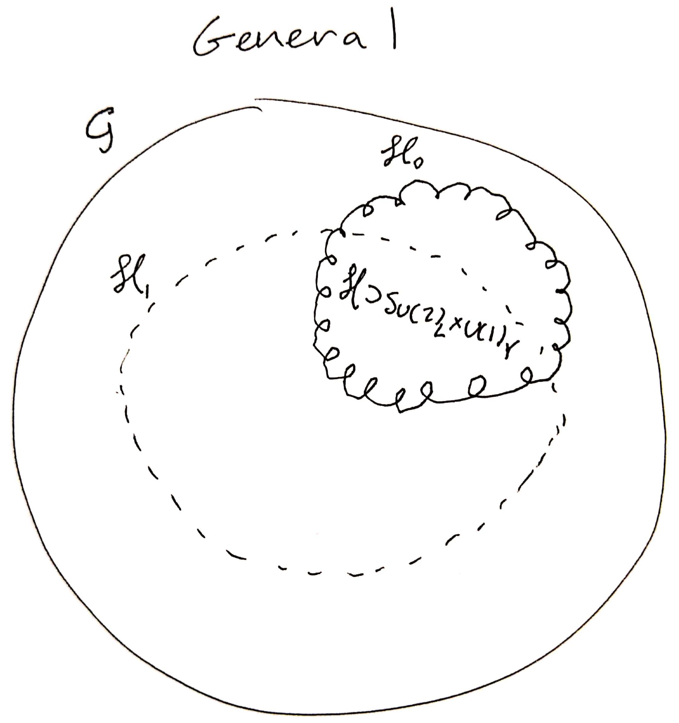
(a)

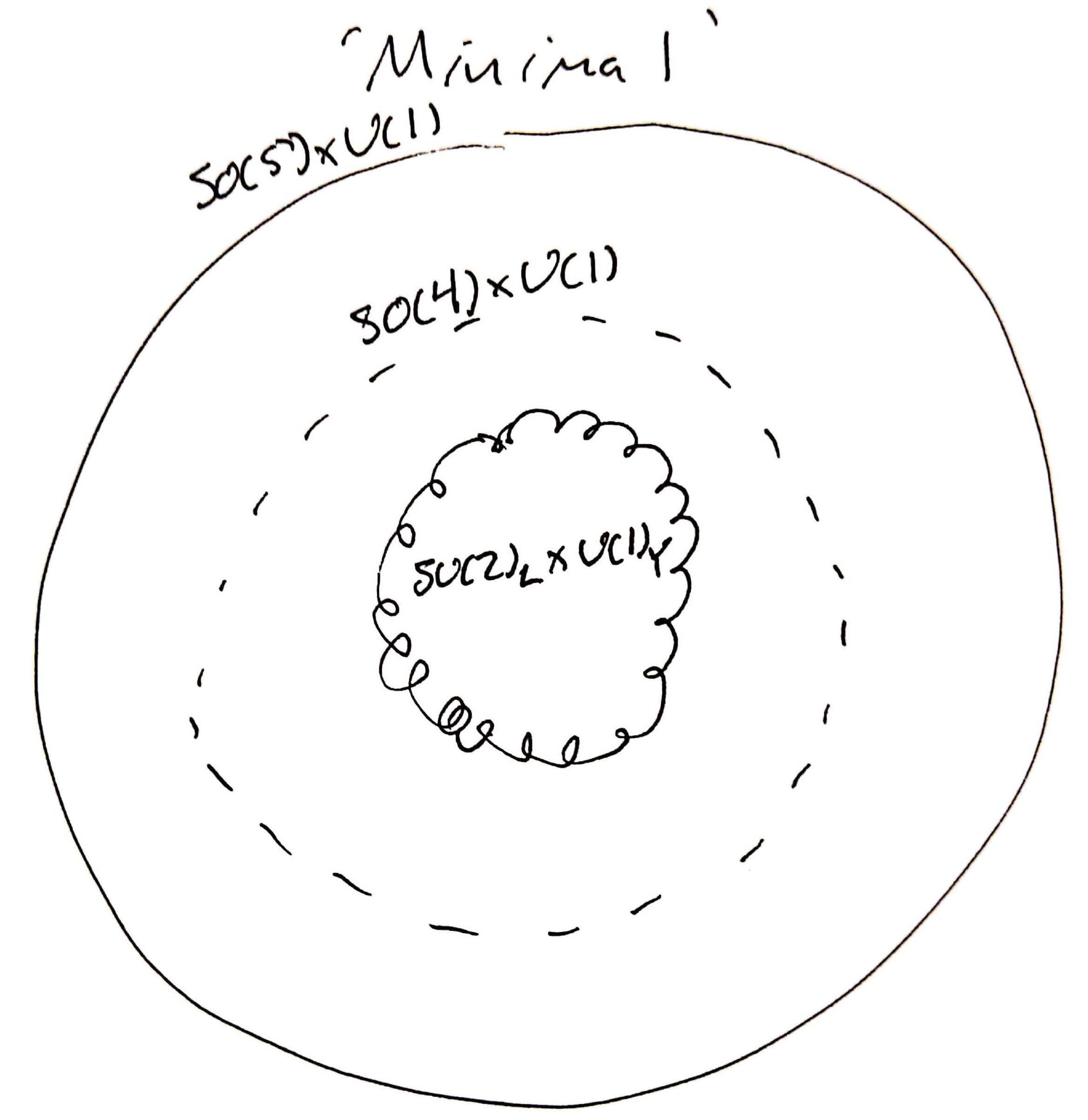
(b)

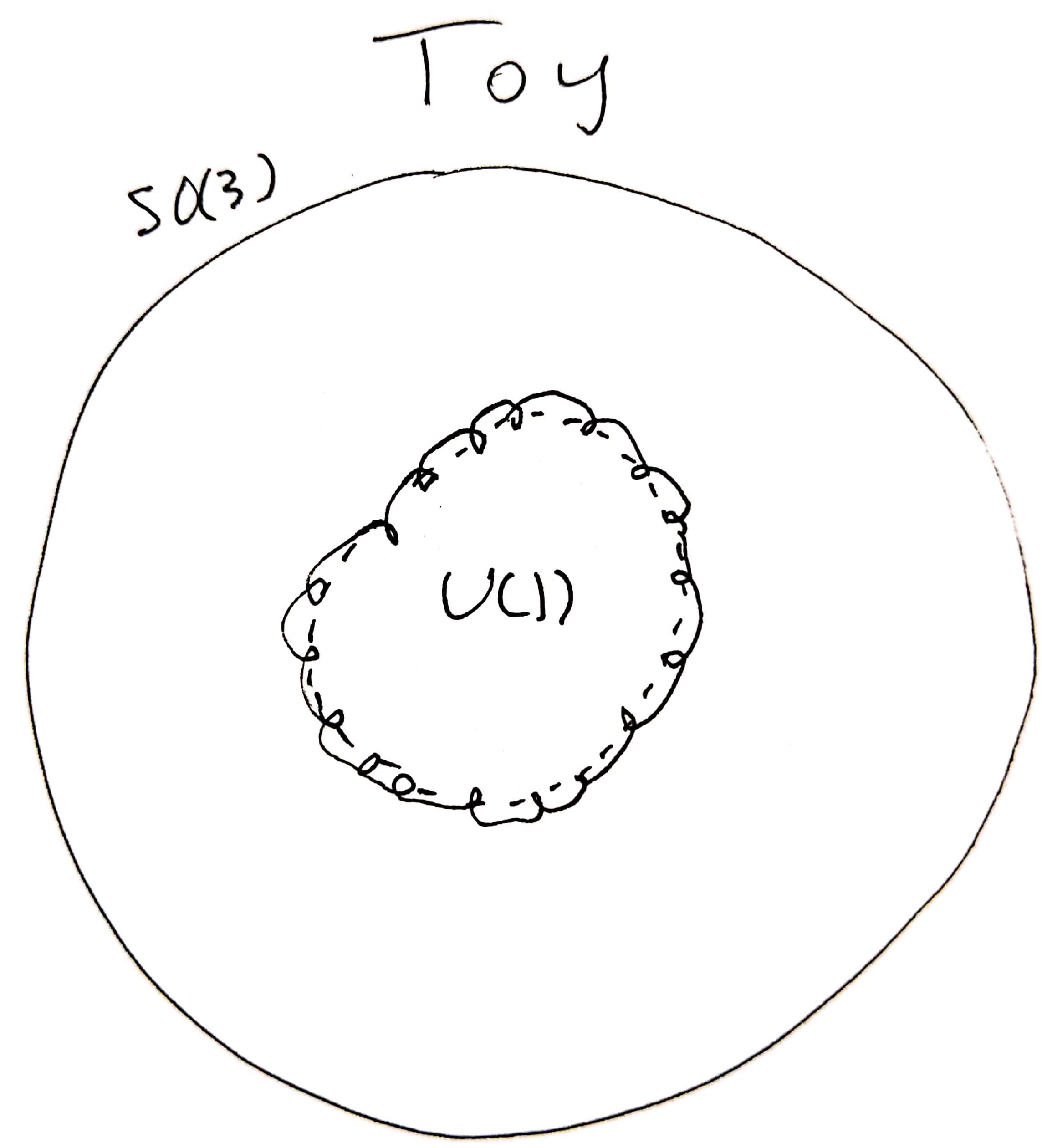
(c)

Figure 5: In (a), the general symmetry setup for a composite Higgs model. Solid lines are the UV symmetries, with the global symmetry enclosed in the smooth circle and the gauge symmetry in the loopy circle. The symmetry group after confinement is dashed. In (b), the same structure applied to the ‘minimal’ model of [257]. In (c), the composite Abelian Higgs toy model discussed in [258], where the symmetry group after confinement coincides with the gauge group.

To evince the ideas in the simplest scenario possible, we’ll discuss an even simpler model for a composite pNGB which then breaks a $U(1)$ gauge symmetry. This is just a toy model to understand the features, which has already been kindly worked out in the extensive review from Panico & Wulzer [258], and which we’ll call a ‘composite Abelian Higgs’ model. To find the most minimal model we’ll ask for a composite pNGB which breaks the smallest continuous gauge symmetry, $U(1)$, for which we simply need two uneaten degrees of freedom (since a charged scalar is necessarily complex). We can make the even more minimal choice $\mathcal{H}_{0}=\mathcal{H}_{1}=\mathcal{H}$, as we’re not worried about having additional unbroken global symmetries. Since $\left[U(1)\right]=1$, we then just need to choose a group $\mathcal{G}$ with at least $\left[\mathcal{G}\right]=3$ to get the right number of pNGBs. We’ll study the breaking $SO(3)\rightarrow SO(2)\simeq U(1)$, which is especially nice because we have geometric intuition for the Lie algebras of these groups.

We’ll study this using a ‘linear sigma model’, of which the ‘chiral Lagrangian’ describing the QCD pions is the most familiar example. Much of the general technology was developed by Callan, Coleman, Wess & Zumino [259, 260], and some modern introductions to this technology can be found in Schwartz’ textbook [22], in a pedagogical review of Little Higgs models by Schmaltz & Tucker-Smith [261], and in exhaustive detail in the review by Scherer [262]. The big idea is one of bottom-up effective field theory: Given knowledge of the symmetry-breaking structure, we can cleverly parametrize our fields to easily see the structure of the Lagrangian which is demanded both before and after symmetry-breaking.

In our case we must start with an $SO(3)$-invariant Lagrangian of a fundamental field $\vec{\Phi}$, which is a familiar $3d$ vector.

$$-\mathcal{L}=\frac{1}{2}\partial_{\mu}\vec{\Phi}^{\intercal}\partial^{\mu}\vec{\Phi}+\frac{g_{\star}^{2}}{8}\left(\vec{\Phi}^{\intercal}\vec{\Phi}-f^{2}\right)^{2},$$ (41)

where $SO(3)$ rotations act as $\vec{\Phi}\rightarrow g\cdot\vec{\Phi}$ with $g=\exp{i\alpha_{A}T^{A}}$, where $T^{A}$, $A=1..3$ are the generators of $SO(3)$. The potential of $\vec{\Phi}$ is minimized for $\left\langle\left|\left|\vec{\Phi}\right|\right|\right\rangle=f^{2}$, so $\vec{\Phi}$ gets a nonzero vev and the symmetry is broken down to rotations keeping $\left\langle\vec{\Phi}\right\rangle$ fixed, which is simply $U(1)$. There are a two-sphere worth of vacua corresponding to possible angles for $\left\langle\vec{\Phi}\right\rangle$, which parametrize the Goldstone directions. We can make the split between broken and unbroken generators explicit by parametrizing our field as

$$\vec{\Phi}=\exp{\left(i\frac{\sqrt[\ ]{2}}{f}\Pi_{i}(x)\hat{T}^{i}\right)}\begin{bmatrix}0\\ 0\\ f+\sigma(x)\end{bmatrix}=(f+\sigma)\begin{bmatrix}\sin\left(\frac{\Pi}{f}\right)\frac{\vec{\Pi}}{\Pi}\\ \cos\left(\frac{\Pi}{f}\right)\end{bmatrix}$$ (42)

where in the first equality $\hat{T}^{i}$ are the two broken generators, $\Pi_{i}(x)$ are the massless Goldstones corresponding to fluctuations along the vacuum manifold, and $\sigma(x)$ is the massive ‘radial mode’ giving fluctuations about the vev. We eschew writing down the generators explicitly and assert that in this case one finds the compact latter expression, with $\Pi=\sqrt[\ ]{\vec{\Pi}^{\intercal}\vec{\Pi}}$. We can find an explicit expression for the interaction of the Goldstones and the radial modes by simply plugging this parametrization into the Lagrangian above. We indeed find a mass for $\sigma$ of $m_{\sigma}=g_{\star}f$, massless pions $\vec{\Pi}$ and a tower of all possible interactions between these fields which are consistent with the symmetries.

We now have a theory of massless scalars transforming under an unbroken symmetry; our pions form a doublet of $SO(2)$ transforming as $\vec{\Pi}\rightarrow\exp{(i\alpha\sigma_{2})}\vec{\Pi}$, corresponding to rotations about the unbroken $SO(3)$ generator. We can complexify by introducing $H\equiv\frac{1}{\sqrt[\ ]{2}}(\Pi_{1}-i\Pi_{2})$ to view $SO(2)\simeq U(1)$ as acting $H\rightarrow\exp{(i\alpha)}H$. As it stands, $H$ is an exact Goldstone boson, so cannot pick up a potential to then itself get a vev and break $U(1)$. However, when we gauge a $U(1)$ subgroup of our original $SO(3)$ global symmetry we’re introducing explicit breaking of the symmetry and resultingly $H$ becomes a pNGB and can pick up a mass. The tree-level effect of this gauging is simply to upgrade derivatives to gauge covariant derivatives, $\partial_{\mu}\vec{\Pi}\rightarrow D_{\mu}\vec{\Pi}=(\partial_{\mu}-ieA_{\mu}\sigma_{2})\vec{\Pi}$.

Now as a result of $SO(3)$ rotations no longer being an exact symmetry, $H$ is free to pick up a potential, which in general will be radiatively generated as a result of this gauging. It is easy to draw diagrams in which loops of our $U(1)$ gauge bosons generate a nonzero mass and quartic for $H$, as in Figure 6, and in a realistic model the corrections from loops of top quarks will be especially important. These loop diagrams come along with an obvious cutoff: Above the compositeness scale $f$, the fields $\vec{\Phi}$ no longer exist in the spectrum. There is a beautiful general method for deriving the radiatively-generated potential for $H$ by resumming the one-loop diagrams with various numbers of external $H$ legs, known as the Coleman-Weinberg potential [263].

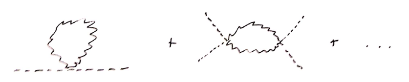
Figure 6: Representative diagrams contributing to the one-loop effective potential for a charged scalar.

Unfortunately, absent any of other structure, finding $v/f\ll 1$ still requires some degree of cancellation between various contributions to the potential of $H$. However any amount of $v/f<1$ will help alleviate the pressure from electroweak precision observables which thus far look empirically as expected for an elementary Higgs field, while still retaining the benefit of forbidding corrections to the Higgs mass above $f$. But one still can’t get away from requiring lots of structure near the electroweak scale, which has not (yet) been observed.

There are a variety of important aspects and interesting directions we do not have the space to discuss. Even past understanding the best sorts of group structures to which to apply this strategy, it is clearly important to understand the sorts of field theories which can confine to break $\mathcal{G}\rightarrow\mathcal{H}_{1}$, as well as the detailed structure of the potential radiatively-generated by SM fields. Then it’s important to explore the possibility of a natural structure which dictates $v/f<1$—while there has been much work on this, we mention in particular the interesting strategy of ‘collective’ symmetry breaking in which a symmetry is broken only by an interplay between different couplings. This class of models is known as the ‘Little Higgs’ [261, 264, 265, 266, 267, 268], and can be seen as a purely four-dimensional application of the strategy of nonlocal symmetry breaking through ‘nonlocality in theory space’ [269, 270], which is a fascinating topic. The TASI notes by Csaki, Lombardo, Telem [271] provide a pedagogical introduction to these topics.

Finally, let me mention that composite Higgs models may be understood as being dual to a novel class of extra-dimensional models known as Randall-Sundrum models [272, 273]. Unlike in the simple cases we discussed in Section 2, in these models the spacetime does not have a product structure (as did $\mathcal{M}_{4}\times K$) and the geometry is said to be ‘non-factorizable’. In this scenario our four-dimensional universe is seen as a brane living on one end of a five-dimensional orbifold of anti-de Sitter space. The minuteness of the electroweak scale compared to the Planck scale is a result of a large fifth-dimensional AdS ‘warp factor’ between the brane we live on (the ‘IR brane’) and the brane on the other end of the space (the ‘UV brane’). As in Section 2, this trades the electroweak hierarchy into a geometric hierarchy, but now in AdS we can find novel, natural ways of generating such a hierarchy of scales [274, 275]. Furthermore, embedding our universe into an AdS spacetime means we can take advantage of the enormously powerful program of AdS/CFT holography, which enables us to study the strong-coupling phenomena of composite Higgs models via their weakly-coupled gravitational duals. Pedagogical introductions to holography can be found in lecture notes from Sundrum [276] and Kaplan [277], and with more background in the textbook by Ammon & Erdmenger [278]. That machinery is not all necessary to appreciate the workings of Randall-Sundrum models, though, and there are a wide variety of great lectures notes aimed at particle theorists, for example those of Sundrum [279], Csaki & Tanedo [280], and Gherghetta [281].

Chapter 3 The Loerarchy Problem

The great tragedy of science — the slaying of a beautiful hypothesis by an ugly fact.

Thomas Henry Huxley
Biogenesis and Abiogenesis (1870) [282]

1 The ‘Little Hierarchy Problem’

We’ve seen in Chapter 2 a cadre of theories which can produce a light scalar naturally, and there’s one feature all the classic approaches have in common: they predict new states with Standard Model charges close to the mass of the Higgs. This is seemingly inevitable simply from the structure of effective field theory—whatever extra structure protects the Higgs mass at UV scales must be broken close to the electroweak scale to allow the Standard Model, which does not have that extra structure. This feature means that smashing together protons at scales much greater than the electroweak scale would surely reveal the physics of whatever mechanism solves the hierarchy problem. And so the Large Hadron Collider was eagerly awaited to tell us which of these ideas was correct.

Yet even years before the LHC turned on, those who could clearly read the tea leaves were realizing that something was amiss with our naturalness expectations (see e.g. the ‘LEP paradox’ [283], also [284]), and exploring the idea that supersymmetry would not show up to solve the hierarchy problem (e.g. ‘split supersymmetry’ [285, 286, 287]). Perhaps there was something else present which made weak-scale supersymmetry unnecessary for protecting the Higgs.

Of course the LHC has been a fantastic success. It has confirmed for us the existence of a light Higgs resonance that looks SM-like, and made many great measurements of the SM besides. But rather than revealing to us which TeV-scale new physics kept the Higgs light, we’ve instead had a march of increasingly powerful constraints on new particles which couple to the Standard Model.

These null results for physics beyond the Standard Model from run 1 of the LHC rapidly popularized the idea that something else might be responsible for stabilizing the Higgs mass at the electroweak scale up to a higher scale where, say, supersymmetry came in. This line of thinking is termed the ‘Little Hierarchy Problem’—the idea being that one of those classic solutions would appear at $\Lambda\sim 10\text{ TeV}$ to solve the ‘Big Hierarchy Problem’ and explain why the Higgs mass was not at the Planck scale, leaving a smaller hierarchy of a couple orders of magnitude between $m_{H}$ and $\Lambda$ unexplained. Perhaps rather than minimal supersymmetry there was another module which provided this last bit of protection. But this has to be a special module to protect the Higgs mass without introducing new colored particles.

1 The Twin Higgs

The first such proposal in fact appeared before the LHC had even turned on. The mirror twin Higgs (MTH) [288] introduces a second copy of the SM gauge group and states related to ours by a $\mathbb{Z}_{2}$ symmetry. Since these ‘twin’ states are neutral under the SM gauge group, they are subject only to indirect bounds from precision Higgs coupling measurements. The two sectors are connected solely by Higgs portal-type interactions between the two $SU(2)$ doublet scalars. Subject to conditions on the quartic coupling, the Higgs sector enjoys an approximate $SU(4)$ global symmetry, and the breaking of this symmetry leads naturally to a pseudo-Nambu Goldstone boson. Seemingly magically, this structure is accidentally respected by the quadratically-divergent one-loop corrections to the Higgs potential, and the pNGB continues to be protected through one-loop from large corrections to its mass. The Twin Higgs thus allows the postponement of a solution to the ‘Big Hierarchy Problem’ until scales a loop factor $16\pi^{2}\sim\mathcal{O}(100)$ above the Higgs mass.

While the space of Neutral Naturalness models has now been explored more thoroughly and we will discuss some generalities below, the mirror twin Higgs remains perhaps the most aesthetically pleasing of all these approaches and serves as a useful avatar for this general strategy. As a result, in Chapter 4 we consider cosmological signatures of the MTH specifically, so we give here a more-detailed introduction to the twin Higgs in particular. This is necessarily slightly more technical than the rest of this chapter, so the reader who is not planning on reading Chapters 4 or 5 in detail may skip ahead $\sim 3$ pages to Section 2 without loss of continuity.

The scalar potential in this model is best organized in terms of the accidental $SU(4)$ symmetry involving the $SU(2)$ Higgs doublets of the SM and twin sectors, $H_{A}$ and $H_{B}$. The general tree-level twin Higgs potential is given by (see e.g. [289])

$$V(H_{A},H_{B})=\lambda(|H_{A}|^{2}+|H_{B}|^{2}-f^{2}/2)^{2}+\kappa(|H_{A}|^{4}+|H_{B}|^{4})+\sigma f^{2}|H_{A}|^{2}.$$ (1)

The first term respects the accidental $SU(4)$ global symmetry, as can be seen by writing it in terms of $\mathcal{H}=\left(H_{A},H_{B}\right)^{\intercal}$, which transforms as a complex $SU(4)$ fundamental. The second term breaks $SU(4)$ but preserves the $\mathbb{Z}_{2}$ and the final term softly breaks the $\mathbb{Z}_{2}$. In order for the $SU(4)$ to be a good symmetry of the potential, we require $\kappa,\sigma\ll\lambda$.

However, the gauging of an $SU(2)\times SU(2)$ subgroup constitutes explicit breaking of the $SU(4)$, so we should worry about whether quantum corrections reintroduce large masses for the would-be Goldstones when $SU(4)$ is broken. But writing down the one-loop corrections reveals a fortuitous accidental symmetry. The one-loop effective scalar potential gets the following leading corrections from the gauge bosons at the quadratic level:

$$V_{1-\text{loop}}(H_{A},H_{B})\supset\frac{9g_{2,A}^{2}}{32\pi^{2}}\Lambda^{2}|H_{A}|^{2}+\frac{9g_{2,B}^{2}}{32\pi^{2}}\Lambda^{2}|H_{B}|^{2}+\text{ subleading}\underset{\mathbb{Z}_{2}}{\rightarrow}\frac{9g_{2}^{2}}{32\pi^{2}}\Lambda^{2}|\mathcal{H}|^{2},$$ (2)

where we see explicitly that if the $\mathbb{Z}_{2}$ symmetry is good at the level of the gauge couplings, then these largest one-loop corrections continue to respect the $SU(4)$. It is easy to see from here by power counting that this holds for all the quadratically-divergent pieces so long as the $\mathbb{Z}_{2}$ is a good symmetry for the interactions involved.

There is radiative $SU(4)$-breaking at the level of the quartic, since the $\mathbb{Z}_{2}$ symmetry no longer suffices to form the Higgses into an $SU(4)$ invariant. The coupling $\kappa$ should naturally be of the order of these corrections, the largest of which comes from the Yukawa interactions with the top/twin top, $\kappa\sim 3y_{t}^{4}/(8\pi^{2})\log(\Lambda/m_{t})\sim 0.1$ for a cut-off $\Lambda\sim 10$ TeV ($y_{t}$ being the top quark Yukawa coupling and $m_{t}$ its mass). Requiring $\lambda\gg\kappa$ therefore implies $\lambda\gtrsim 1$. As the SM and twin isospin gauge groups are disjoint subgroups of the $SU(4)$, the spontaneous breaking of the $SU(4)$ coincides with the SM and twin electroweak symmetry breaking. This gives seven Goldstone bosons, six of which are ‘eaten’ by the $SU(2)$ gauge bosons of the two sectors, which leaves one Goldstone remaining. This will acquire mass through the breaking of the $SU(4)$ that is naturally smaller than the twin scale $f$. For future reference, it is convenient to define the real scalar degrees of freedom in the gauge basis as $h_{A}=\frac{1}{\sqrt[\ ]{2}}\Re(H_{A}^{0})-v_{A}$ and $h_{B}=\frac{1}{\sqrt[\ ]{2}}\Re(H_{B}^{0})-v_{B}$, where $\langle H_{A}^{0}\rangle=v_{A}$ and $\langle H_{B}^{0}\rangle=v_{B}$.

The surviving Goldstone boson should be dominantly composed of the $h_{A}$ gauge eigenstate in order to be SM-like. The soft $\mathbb{Z}_{2}$-breaking coupling $\sigma$ is required to tune the potential so that the vacuum expectation values (vevs) are asymmetric and that the Goldstone is mostly aligned with the $h_{A}$ field direction. The (unique) minimum of the Twin Higgs potential (1) occurs at $v_{A}\approx\frac{f}{2}\sqrt[\ ]{\frac{\lambda(\kappa-\sigma)-\kappa\sigma}{\lambda\kappa}}$ and $v_{B}\approx\frac{f}{2}\sqrt[\ ]{\frac{\sigma+\kappa}{\kappa}}$. The required alignment of the vacuum in the $H_{B}$ direction occurs if $\sigma\approx\kappa$, which has been assumed in these expressions for the minimum. The consequences of this are that $v_{A}\approx v/\sqrt[\ ]{2}$ and $v_{B}\approx f/\sqrt[\ ]{2}\gg v$ (where $v$ is the vev of the SM Higgs, although $v_{A}\approx 174$ GeV is the vev that determines the SM particle masses and electroweak properties), so that the SM-like Higgs $h$ is identified with the Goldstone mode and is naturally lighter than the other remaining real scalar, a radial mode $H$ whose mass is set by the scale $f$. The component of $h$ in the $h_{B}$ gauge eigenstate is $\delta_{hB}\approx v/f$ (to lowest order in $v/f$). Measurements of the Higgs couplings restrict $f\gtrsim 3v$ [290, 289], and the Giudice-Barbieri tuning of the weak scale associated with this asymmetry is of order $f^{2}/2v^{2}$.

The spectrum of states in the broken phase consists of a SM-like pseudo-Goldstone Higgs $h$ of mass $m_{h}^{2}\sim 8\kappa v^{2}$, a radial twin Higgs mode $H$ of mass $m_{H}^{2}\sim 2\lambda f^{2}$, a conventional Standard Model sector of gauge bosons and fermions and a corresponding mirror sector. The masses of quarks, gauge bosons, and charged leptons in the twin sector are larger than their Standard Model counterparts by $\sim f/v$, while the twin QCD scale is larger by a factor $\sim\left(1+\log(f/v)\right)$ due to the impact of the higher mass scale of heavy twin quarks on the renormalisation group (RG) evolution of the twin strong coupling. The relative mass of twin neutrinos depends on the origin of neutrino masses, some possibilities being $\sim f/v$ for Dirac masses and $\sim f^{2}/v^{2}$ for Majorana masses from the Weinberg operator. Mixing in the scalar sector implies that the SM-like Higgs couples to twin sector matter with an $\mathcal{O}(v/f)$ mixing angle, as does the radial twin Higgs mode to Standard Model matter. These mixings provide the primary portal between the Standard Model and twin sectors.

The Goldstone Higgs is protected from radiative corrections from $\mathbb{Z}_{2}$-symmetric physics above the scale $f$. While the mirror Twin Higgs addresses the little hierarchy problem, it does not address the big hierarchy problem, as nothing stabilizes the scale $f$ against radiative corrections. However, the scale $f$ can be stabilized by supersymmetry, compositeness, or perhaps additional copies of the twin mechanism [291] without requiring new states beneath the TeV scale. Minimal supersymmetric UV completions can furthermore remain perturbative up to the GUT scale [292, 293].

As mentioned, the collider constraints on twin Higgs models are very mild and pertain mostly to a lower bound on the soft breaking of the $\mathbb{Z}_{2}$. In this respect, the Twin Higgs naturally reconciles the observation of a light Higgs with the absence of evidence for new physics thus far at the LHC. The primary challenge to these models comes from cosmology due to the effects of additional light particles on the cosmic microwave background. We will discuss these issues in Chapter 4 and propose a natural resolution.

2 Neutral Naturalness or The Return Of The Orbifold

More broadly, the twin Higgs is just the simplest example of the more general ‘Neutral Naturalness’ paradigm in which the states responsible for stabilizing the electroweak scale are not charged under (some of) the Standard Model (SM) gauge symmetries [288, 294, 295, 296, 297, 298, 299, 300, 301, 302, 303, 304, 305], thus explaining the lack of expected signposts of naturalness.

In the symmetry-based solutions to the hierarchy problem discussed in Chapter 2, modifications of the Higgs mass were technically natural as a result of a continuous symmetry which commuted with the SM gauge groups. This naïvely seems necessary to ensure that the necessary degrees of freedom are present and couple to the Higgs with the right strength to cancel divergences. How is the top quark contribution $\propto N_{c}y_{t}$ (where $N_{c}$ is the number of colors) to be canceled if not by another colored particle with the same coupling to the Higgs, which gives the opposite contribution? Well we saw above that the twin Higgs nevertheless works with a quark charged under a separate gauge group. Indeed, at one-loop $N_{c}$ is really just a ‘counting factor’ and we are free to get those three opposite-sign contributions in a variety of ways. To some extent the space of Neutral Naturalness models is an exercise in interesting ways to find that color factor. We’ll be able to see that picture more clearly in the language of orbifold projection, which will also give us good reason to expect that these models with naïvely strange symmetries in fact do have nice UV completions.

In Section 3 we saw how orbifolds could be useful dynamically—that is, in affording a higher-dimensional, symmetric theory which at low energies looks like a less symmetric, four-dimensional theory due to boundary conditions imposed by the orbifold discrete symmetries. But these theories had interesting properties in their low-energy behavior below the scale of compactification; we didn’t need to make reference to their origins in studying them.

Now we want to understand the variety of low energy theories we can get very generally, but only at the level of the zero-mode spectrum. Rather than decomposing our fields into modes and integrating over the compact manifold and noticing that only those fields invariant under the orbifold symmetry are left with zero-modes, we’re going to skip to the answer and look at the spectrum of fields left invariant under our discrete symmetry. We’ll find that these theories have enhanced symmetry properties at one loop.

The underlying reason lies in the ‘orbifold correspondence’ in large $N$ gauge theories [306, 307, 308]. Given a ‘mother’ field theory, you can create a ‘daughter’ theory by embedding some given discrete symmetry in the symmetries of the mother theory and projecting out states which are not invariant under that discrete symmetry; we call this process ‘orbifolding’. Then at leading order in large $N$, the correlation functions of the daughter theory match those of the mother theory. This is nothing short of amazing—a theory with no supersymmetry to speak of can nevertheless ‘accidentally’ exhibit supersymmetric behavior at leading order.

The general case of the orbifold correspondence and how to construct Neutral Naturalness models is beautiful and I do recommend reading [306, 295, 309], but the group theory required for a full discussion would be too large a detour from our main narrative. Fortunately we can get a good sense for what’s going on by considering a few explicit examples, which will not require much mathematical machinery.

Example 1: Folded Supersymmetry

Let’s first consider the example of ‘Folded Supersymmetry’ [295] which was the first Neutral Naturalness model constructed explicitly via orbifolding. The idea is precisely to consider a supersymmetric theory and orbifold project onto a theory with no explicit supersymmetry but in which supersymmetric cancellations still occur at one loop. As a pedagogical example, consider an $\mathcal{N}=1$ supersymmetric $U(2N)_{C}$ gauge theory with $2N$ flavors of left and right fundamental chiral superfields $Q=(\tilde{q},q)$ which enjoy a $U(2N)_{F,L}\times U(2N)_{F,R}$ global flavor symmetry. Let’s decree also that the theory respects $R$-symmetry. We will orbifold by the discrete group $\mathbb{Z}_{2}$ as before, but we must choose how to embed the $\mathbb{Z}_{2}$ in each of these symmetry groups. That is, our original ‘mother’ theory is invariant under a large symmetry group $U(2N)_{C}\times U(2N)_{F,L}\times U(2N)_{F,R}\times U(1)_{R}$, which contains many $\mathbb{Z}_{2}$ subgroups, and we must decide precisely which $\mathbb{Z}_{2}$ we want to orbifold by. We choose the following embeddings:

$$\mathbf{C}=\begin{pmatrix}\mathds{1}_{N}&0\\ 0&-\mathds{1}_{N}\end{pmatrix},\qquad\mathbf{F}=\begin{pmatrix}\mathds{1}_{N}&0\\ 0&-\mathds{1}_{N}\end{pmatrix},\qquad\mathbf{R}=(-1)^{F},$$ (3)

where the first matrix is in color-space, the second is in flavor-space, and the third transformation is by fermion number. Each of these generates a $\mathbb{Z}_{2}$ subgroup of one of the symmetry factors of the mother theory. To see which fields are invariant under this $\mathbb{Z}_{2}$, we must only act them on the fields and see how they transform. Gauge bosons $A_{\mu}$ and their superpartner gauginos $\lambda$ are in the adjoint of the gauge group. Indexing $A,B=1..N$ separately over the two halves of the gauge indices, we have

$$A_{\mu} =\begin{pmatrix}A_{\mu,AA}&A_{\mu,AB}\\ A_{\mu,BA}&A_{\mu,BB}\end{pmatrix}\rightarrow\mathbf{C}\begin{pmatrix}A_{\mu,AA}&A_{\mu,AB}\\ A_{\mu,BA}&A_{\mu,BB}\end{pmatrix}\mathbf{C}^{\dagger}\mathds{1}_{R}=\begin{pmatrix}+A_{\mu,AA}&-A_{\mu,AB}\\ -A_{\mu,BA}&+A_{\mu,BB}\end{pmatrix}$$ (4)

$$\lambda =\begin{pmatrix}\lambda_{AA}&\lambda_{AB}\\ \lambda_{BA}&\lambda_{BB}\end{pmatrix}\rightarrow\mathbf{C}\begin{pmatrix}\lambda_{AA}&\lambda_{AB}\\ \lambda_{BA}&\lambda_{BB}\end{pmatrix}\mathbf{C}^{\dagger}(-\mathds{1})_{R}=\begin{pmatrix}-\lambda_{AA}&+\lambda_{AB}\\ +\lambda_{BA}&-\lambda_{BB}\end{pmatrix}$$ (5)

where the difference here is because of the different $R$ transformations. We see that if we project down to only those states invariant under this transformation, our gauge group dissolves from $U(2N)_{C}$ down to disconnected pieces $U(N)_{C}\times U(N)_{C}$. We see that embedding the $\mathbb{Z}_{2}$ non-trivially in the $R$-symmetry group means the daughter theory will be non-supersymmetric. The superpartners of our gauge fields are no longer present, but rather the gauginos have been twisted into bifundamentals under the two gauge factors. In the matter sector, letting $a,b=1..N$ similarly index the two halves of the flavor indices and writing the fields as matrices in a combined color and flavor space, we have

$$\tilde{q} =\begin{pmatrix}\tilde{q}_{Aa}&\tilde{q}_{Ab}\\ \tilde{q}_{Ba}&\tilde{q}_{Bb}\end{pmatrix}\rightarrow\mathbf{C}\begin{pmatrix}\tilde{q}_{Aa}&\tilde{q}_{Ab}\\ \tilde{q}_{Ba}&\tilde{q}_{Bb}\end{pmatrix}\mathbf{F}^{\dagger}\mathds{1}_{R}=\begin{pmatrix}+\tilde{q}_{Aa}&-\tilde{q}_{Ab}\\ -\tilde{q}_{Ba}&+\tilde{q}_{Bb}\end{pmatrix}$$ (6)

$$q =\begin{pmatrix}q_{Aa}&q_{Ab}\\ q_{Ba}&q_{Bb}\end{pmatrix}\rightarrow\mathbf{C}\begin{pmatrix}q_{Aa}&q_{Ab}\\ q_{Ba}&q_{Bb}\end{pmatrix}\mathbf{F}^{\dagger}(-\mathds{1})_{R}=\begin{pmatrix}-q_{Aa}&+q_{Ab}\\ +q_{Ba}&-q_{Bb}\end{pmatrix}.$$ (7)

Again we see that we have broken supersymmetry. The flavor group has also broken down to $U(N)_{F,L}\times U(N)_{F,L}$ and the invariant states are squarks which are bifundamentals under ‘diagonal’ combinations of the gauge and flavor groups, and quarks which are bifundamentals under the ‘off-diagonal’ combinations.

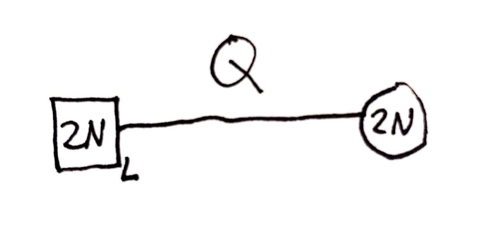
(a)

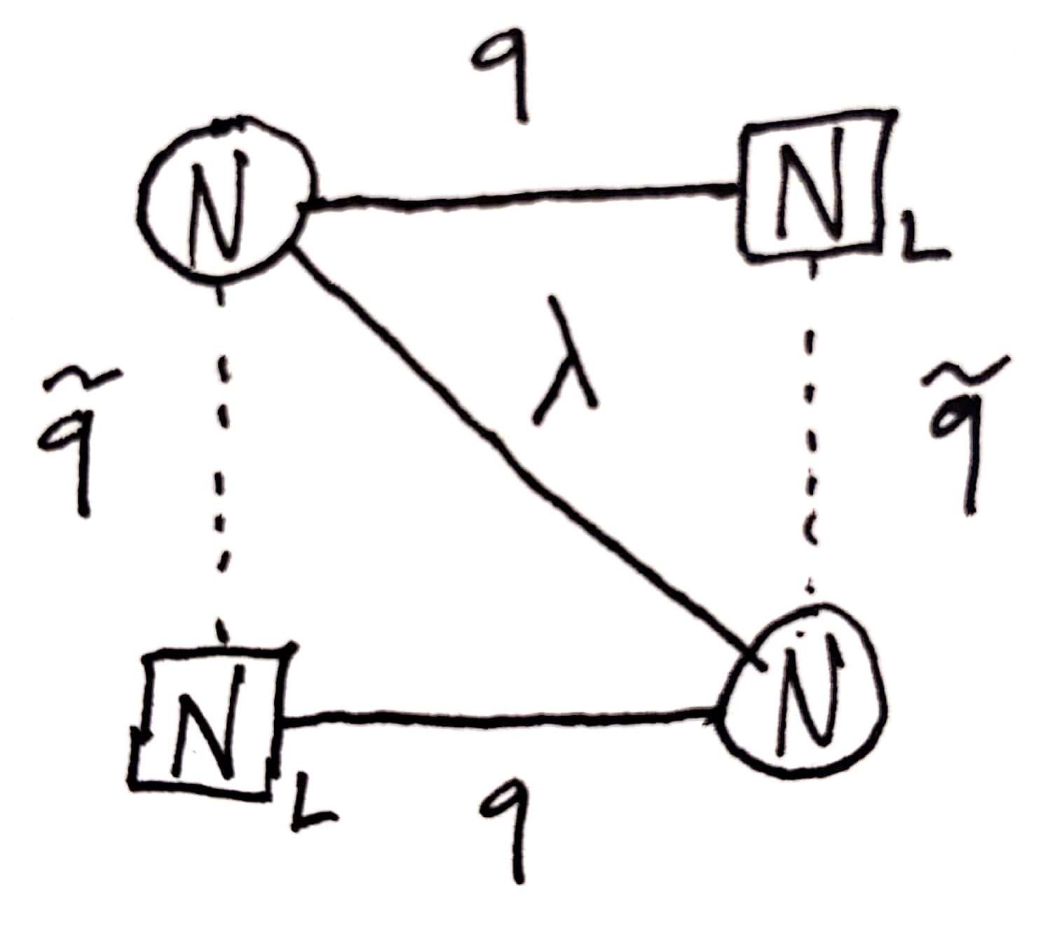
(b)

Figure 1: In (a), a quiver diagram for the (left-chiral fields in) the mother theory. A circle corresponds to a gauge symmetry and a square to a flavor symmetry. Lines between denote bifundamentals, which here represents a full chiral supermultiplet. In (b), a quiver diagram for the orbifold daughter theory described in the text. The gauge and flavor groups have been divided into two distinct groups each, and the degrees of freedom in the chiral and vector supermultiplet have been shuffled around.

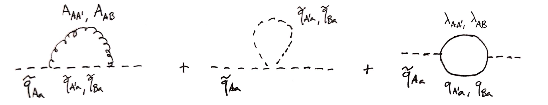
Figure 2: Representative diagrams contribution to the one-loop mass correction of a scalar in the supersymmetric mother theory. The daughter theory projects out some of the internal states of each diagram in a pattern that is non-supersymmetric but still enforces cancellations.

It is not too hard to roughly see the magic of how the orbifold-projected theory continues to protect scalar masses. Draw the one-loop the diagrams in the mother theory which would contribute to a calculation of the mass of, say, $\tilde{q}_{Aa}$, as in Figure 2. In the mother theory we know there are no quadratic corrections by supersymmetry. In the daughter theory, half of each sort of diagram will be eliminated by the orbifold projection, so it’s clear that there will still be no quadratic divergences. But because it is different internal states that have been eliminated for different classes of diagrams, the daughter theory has no supersymmetry to speak of! Again, as we saw in the example of the twin Higgs, the magic is in that at one-loop we really only need to get the counting right, and so we can use orbifolding to construct theories which do that in clever ways.

The structure of the theory can be succinctly summarized in a ‘quiver’ or ‘moose’ diagram where the various symmetry groups correspond to nodes in a graph and the matter is represented by links between these groups which represent their charges, as in Figure 1.

Despite the fact that our daughter theory has no supersymmetry, the orbifold correspondence guarantees that in the $N\rightarrow\infty$ limit the correlation functions have full supersymmetric protection. For finite $N$ the supersymmetric relations are broken, but only by $1/N$ corrections. Going through this explicitly is useful, and pedagogical discussions of it can be found in [306, 298].

Example 2: The $\Gamma$-plet Higgs

We can understand the twin Higgs as the simplest example of a $\Gamma$-siblings Higgs which is the orbifold projection $SU(3\Gamma)\times SU(2\Gamma)\times SU(\Gamma)_{F}/\mathbb{Z}_{\Gamma}$, where the first two factors are gauged and the last is a flavor symmetry. We focus on the sector which contains the Yukawa interaction of the top quark, as the top partners have the most effect on the naturalness of the Higgs. In the mother theory the matter content is:

	$SU(3\Gamma)$	$SU(2\Gamma)$	$SU(\Gamma)_{F}$
$H$	-	$\Box$	$\overline{\Box}$
$Q$	$\Box$	$\overline{\Box}$	-
$u$	$\overline{\Box}$	-	$\overline{\Box}$

where ‘$\Box$’ denotes the fundamental representation and ‘$\overline{\Box}$’ denotes the antifundamental, and we note that the charges allow the operator $y_{t}HQu$. The Abelian generalization of the twin Higgs is found by embedding the $\mathbb{Z}_{\Gamma}$ in these groups as the block-diagonal element $\mathbf{S}_{n}=\text{diag}\left[\mathds{1}_{n},\mathds{1}_{n}\exp(2\pi i/\Gamma),\dots,\mathds{1}_{n}\exp(2\pi ki/\Gamma),\dots,\mathds{1}_{n}\exp(2\pi(\Gamma-1)i/\Gamma)\right]$, where $n=1,2,3$ corresponds to which $SU(n\Gamma)$ factor the element belongs to and $\mathds{1}_{n}$ is the $n\times n$ identity matrix.

The pattern of orbifolding is extremely simple in this example. We write the Higgs field as a matrix of $\Gamma$ columns and $2\Gamma$ rows in blocks of two, with the field in block $i,j$ being $H^{(i)}_{A_{j}}$ where $i$ simply labels the column and $A_{j}=1,2$ is an $SU(2)$ index. Now we can look at how this field transforms under the chosen $\mathbb{Z}_{\Gamma}$,

$$H =\begin{pmatrix}H^{(0)}_{A_{0}}&\dots&H^{(\Gamma-1)}_{A_{0}}\\ \vdots&\ddots&\vdots\\ H^{(0)}_{A_{\Gamma-1}}&\dots&H^{(\Gamma-1)}_{A_{\Gamma-1}}\\ \end{pmatrix}\rightarrow\mathbf{S}_{2}H\mathbf{S}_{1}^{\dagger}$$ (8)

$$\rightarrow\begin{pmatrix}\mathds{1}^{A_{0}}H^{(0)}_{A_{0}}\mathds{1}&\dots&\mathds{1}^{A_{0}}H^{(\Gamma-1)}_{A_{0}}\mathds{1}e^{-2\pi(\Gamma-1)i/\Gamma}\\ \vdots&\ddots&\vdots\\ \mathds{1}^{A_{\Gamma-1}}e^{2\pi(\Gamma-1)i/\Gamma}H^{(0)}_{A_{\Gamma-1}}\mathds{1}&\dots&\mathds{1}^{A_{\Gamma-1}}e^{2\pi(\Gamma-1)i/\Gamma}H^{(\Gamma-1)}_{A_{\Gamma-1}}e^{-2\pi(\Gamma-1)i/\Gamma}\\ \end{pmatrix},$$ (9)

and we see immediately that the only invariant elements are those on the diagonal. It is simple to repeat this for the $Q,u$ fields to find the same feature. Then in this example there are no off-diagonal fields at all, and the daughter theory consists of $\Gamma$ SM-like sectors. These sectors are all identical and so have a $S_{\Gamma}$ rearrangement symmetry, leading to a one-loop quadratic potential of the form

$$V_{1-\text{loop}}\sim c\frac{\Lambda^{2}}{16\pi^{2}}\sum_{i=0}^{\Gamma-1}\left|H^{(i)}_{A_{i}}\right|^{2},$$ (10)

That is, just as in the twin Higgs, the $SU(2\Gamma)$ symmetry of the scalar potential is respected by the one-loop quadratic corrections as a result of the discrete symmetry despite being explicitly broken by the gauge groups. This clearly opens up a much wider space of Neutral Naturalness models where the Higgs is a pseudo-Nambu Goldstone boson and so receives some protection of its mass without new colored particles at the electroweak scale.

The general orbifolding approach to constructing models of Neutral Naturalness was fully laid out in [309, 298], where they in particular explore a ‘regular representation’ embedding of the discrete group into the continuous symmetries of the mother theory.

This approach of orbifolding to find low-energy models with accidental symmetries is useful also because such models come along with guides for how to UV-complete them. When we wrote down the twin Higgs model above, it was perhaps not obvious that there is a nice UV completion of this theory. But now we see that the twin Higgs is an orbifold projection of a $SU(6)\times SU(4)$ gauge theory by $\mathbb{Z}_{2}$, so we expect we can uplift this to a five-dimensional UV completion where the twin Higgs emerges dynamically at low energies from orbifold boundary conditions. So we can confidently study solely the low-energy effective theory of the zero-modes we’ve projected out without worrying explicitly about whether a UV completion exists.

2 The Loerarchy Problem

Modern particle theorists must now confront a new version of the issue of electroweak naturalness. When originally understood, the pressing problem was understanding what sorts of UV structure could protect a scalar from large mass corrections. Of course this structure needed to be broken to get the SM structure in the IR and there’s lots of interesting physics and subtleties on that end as well. But with the structure of the weak scale barely explored, the ways in which this could be done were abundant.

Over the ensuing decades we explored electroweak physics with increasing precision, which has provided invaluable guidance for how the SM structure must appear. Gradually the IR dynamics became more and more constrained to the point where now, as we have emphasized, we have enormous constraints on any appearance of new physics with SM quantum numbers up to mass scales that are often many times the electroweak scale.

We thus have a qualitative change in the electroweak naturalness issue over the past decades. We term the modern, empirical, low-energy puzzle of electroweak naturalness without visible structure around the weak scale as ‘The Loerarchy Problem’, for obvious reasons.

In this language, the little hierarchy problem is just one approach toward this problem, which assumes that one of the classic solutions is just out of reach and another module is needed to postpone the appearance of SM charged particles. While it’s more than worthwhile to continue looking for and exploring those theories, in the face of increasingly powerful LHC data in excellent agreement with the Standard Model it’s worth thinking transversely. As intriguing as the Neutral Naturalness models are, these classes of models rely on one-loop accidents and so do not completely relieve the empirical pressure from a lack of new physics at the energy frontier. Such models are gradually also being constrained by the LHC, so what else are we to do? The maximalist interpretation of the LHC data is that Nature may be leading us to the conclusion that there is no new physics at the weak scale. With every inverse femtobarn of LHC data without a signal of new physics, the impetus for such a paradigm shift becomes stronger.

But how can we generate a scale without additional structure appearing surrounding it? Within the context of effective field theory, decoupling theorems demand that if the RG evolution is to change around a scale $M$ it must be due to fields close to the scale $M$. This was perhaps clearest in dim reg with $\overline{\text{MS}}$, where the beta functions explicitly change solely at mass thresholds, though the Wilsonian approach is more useful for physical intuition. So how are we to break this feature? This undertaking is the maximalist approach to the Loerarchy Problem.

3 Violations of Effective Field Theory

There are more things in heaven and earth, Horatio,
Than are dreamt of in your philosophy.

William Shakespeare
Hamlet, c. 1600 [310]

The line of thought we suggest here is that perhaps the apparent violation of EFT expectations at the weak scale is a sign of the breakdown of EFT itself. Depending on how much background in particle physics one has this statement may seem more or less heretical, but the idea is not as radical as it may at first seem—for one reason, the cosmological constant problem has inspired sporadic reexaminations of the validity of effective field theory in our universe for decades.

The cosmological constant problem is the fine-tuning issue with the other dimensionful parameter in the Standard Model. Just as with the Higgs mass, there is no protective symmetry in the Standard Model for the vacuum energy, and so the natural expectation is $\Lambda\sim M_{\text{pl}}^{4}$, some $120$ orders of magnitude higher than observations suggest. However there’s an important difference in the severity of these problems—for the Higgs, as emphasized in Section 1, the worrisome mass corrections are those from new physics. This is why the severity of the problem has only ratcheted up in recent years, as we have seen nothing to protect the Higgs from BSM mass corrections. But for the vacuum energy, there are finite, calculable, physical contributions in the Standard Model itself! For a start, EWSB by the Higgs yields a contribution $\sim-v^{4}$, and chiral symmetry-breaking yields a contribution $\sim-\Lambda_{QCD}^{4}$. How is it that these can be nearly perfectly canceled off in the late universe?

There have been important attempts to address the cosmological constant problem with a violation of effective field theory, from Coleman’s suggestion [311] that nonlocality induced by wormholes may allow the early universe to be sensitive to late-time requirements to Cohen-Kaplan-Nelson’s suggestion [312] that the Bekenstein bound demands an infrared cutoff on the validity of any EFT. From one perspective, our suggestion to extend this philosophy to the hierarchy problem appears natural in light of its apparent need in cosmology. We can point to an even-more-general motivation with the realization that gravity necessarily violates EFT.

1 Gravity and EFT

The perturbative quantum field theory of the Einstein-Hilbert Lagrangian [313] is quite clearly an effective field theory of a symmetric two-index tensor field which obeys diffeomorphism invariance and with power counting in $1/M_{\text{pl}}$ [314], as we can easily see by writing it out and expanding around flat space $g_{\mu\nu}=\eta_{\mu\nu}+h_{\mu\nu}$:

$$-\mathcal{L}_{EH}=\frac{1}{2M_{\text{pl}}^{2}}\sqrt[\ ]{g}R\sim\partial^{2}h^{2}+\frac{1}{M_{\text{pl}}}\partial^{2}h^{3}+\frac{1}{M_{\text{pl}}^{2}}\partial^{2}h^{4}+\dots$$ (11)

where we have only given the schematic form of the operators in terms of the number of derivatives and linearized gravitational fields they contain, as the full expressions quickly become complicated [315, 316]. Then we may expect that this effective field theory will be a good approximation to infrared gravitational physics until we get to energies close to the Planck scale, at which point the higher-dimensional operators are unsuppressed and we need a UV completion. From this bottom-up approach it’s not clear why gravity should be particularly special. But we can get some insight at a very basic level by thinking about gravitational scattering.

Let’s compare two effective field theories: the four-Fermi theory of the weak interaction below the weak scale $G_{F}^{-1/2}$ and the perturbative theory of quantum gravity below the Planck mass. If we consider scattering two leptons at $\sqrt[\ ]{s}\ll G_{F}^{-1/2}$, we can make very precise predictions by computing in the four-Fermi theory—the possible final states, the differential cross-section; whatever we’d like. And similarly if we scatter two particles at $\sqrt[\ ]{s}\ll M_{\text{pl}}$, we can compute to high precision in quantum gravitational corrections what will happen.

Now inversely, imagine scattering two leptons at $\sqrt[\ ]{s}\gg G_{F}^{-1/2}$ in the four-Fermi theory. At a scale like $10^{15}G_{F}^{-1/2}$, the EFT has obviously broken down and we can say essentially nothing about what this process will look like—any calculation we tried would be hopelessly divergent, and we have no idea what sorts of states might exist at energies that large.

However, what if we scatter two particles at $\sqrt[\ ]{s}\gg M_{\text{pl}}$, say a ridiculously trans-Planckian scale like $10^{15}M_{\text{pl}}$? In this case, in fact, we know what will happen to incredible precision—a black hole will form! This will be a ‘big’ black hole of mass $\gg M_{\text{pl}}$ with a lifetime of order days. It will be well-described by classical general relativity for some macroscopic time, and then semiclassical GR for an $\mathcal{O}(1)$ fraction of the full lifetime. In fact, unless you are interested in incredibly detailed measurements which involve collecting essentially every emitted Hawking quanta (of which there will be $n\sim 10^{30}$ in this case!) and finding their entanglement structure, we know how to describe the evaporation nearly completely.

So something profoundly weird is going on. The key point being that in gravity, the far UV of the theory is controlled by classical, infrared physics. This is obviously a feature that we do not see in other EFTs.

This is not a new idea; it has long been known that gravity contains low-energy effects which cannot be understood in the context of EFT. The fact that black holes radiate at temperatures inversely proportional to their masses [318] necessitates some sort of ‘UV/IR mixing’ in gravity—infrared physics must somehow ‘know about’ heavy mass scales in violation of a naïve application of decoupling. As a perhaps-more-fundamental raison d’être for such behavior, the demand that observables in a theory of quantum gravity must be gauge-(that is, diffeomorphism-)invariant dictates that they must be nonlocal (see e.g. [319, 320, 321, 322, 323]), again a feature which standard EFT techniques do not encapsulate. In view of this, the conventional position is that EFT should remain a valid strategy up to the Planck scale, at which quantum gravitational effects become important. But once locality and decoupling have been given up, how and why are violations of EFT expectations to be sequestered to inaccessible energies? Indeed, the ‘firewall’ argument [324] evinces tension with EFT expectations in semiclassical gravity around black hole backgrounds at arbitrarily low energies and curvatures, as does recent progress finding the Page curve from semiclassical gravity [325, 326, 327, 328, 329, 330].

That quantum gravitational effects will affect infrared particle physics is likewise not a new idea. This has been the core message of the Swampland program [331], which has been cataloging—to varying degrees of concreteness and certainty—ways in which otherwise allowable EFTs may conjecturally be ruled out by quantum gravitational considerations. These are EFTs which would look perfectly sensible and consistent to an infrared effective field theorist, yet the demand that they be UV-completed to theories which include Einstein gravity reveals a secret inconsistency. While this is powerful information, the extent to which the UV here meddles with the IR is relatively minor—just dictating where one must live in the space of infrared theories. Even so, they have been found to have possible applications to SM puzzles, including the hierarchy problem [97, 98, 99, 100, 101, 102, 103, 104, 11, 5, 105].

Let us review briefly the approach to connect the Weak Gravity Conjecture (WGC) [332] to the hierarchy problem. The WGC is one of the earliest and most well-tested Swampland conjectures, its formulation is relatively easy to understand, and it’s emblematic of the way one might try to connect the hierarchy problem to Swampland conjectures in general.

The prime motivation for formulating the WGC was the well-known folklore that quantum gravity does not respect global symmetries. The simple argument for this fact is that ‘black holes have no hair’—the only quantum numbers a black hole has correspond to its mass, spin, and gauge charges. This means that if we make a black hole by smashing together a bunch of neutrons, there is no reason why it cannot decay into solely photons, which violates the global $U(1)_{B-L}$ symmetry of the SM but no gauge symmetries. The authors suggested that the fact that Abelian gauge symmetries smoothly become global symmetries as the gauge coupling vanishes means that something must go wrong with very small gauge couplings as well, so as for the physics to be smooth in this limit.

Another line of thinking for quantum gravity not respecting global symmetries, which connects more closely to the WGC formulation, is based on entropic arguments. If global symmetries could be exact, then we could create a big black hole with an arbitrary global charge, and wait a very very long time while it Hawking evaporates down to the Planck scale. Unlike gauge charges, the global charge does not affect the metric, so the black hole does not shed this charge as it evaporates. We then end up with a Planck-sized black hole with an arbitrarily large global charge, which would necessitate the existence of arbitrarily-many black hole microstates for a fixed-mass black hole. But this is a disaster! In calculating a scattering amplitude one has to sum over all possible intermediate states, in principle including black holes. These effects are surely Boltzmann-suppressed by enormous amounts, but if there are an infinite number of possible black holes then any nonzero contribution from a single black hole will lead to a divergence. A cuter (albeit somewhat tongue-in-cheek) ‘hand waving argument’ is provided by [333]: Were there incredibly large numbers of super-Planckian states which could populate a thermal bath, a vigorous wave of your hand would produce them in Unruh radiation, and you could feel them against your hand as they evaporated.

Now if we have a gauge symmetry, there are no longer Planck-sized black holes with arbitrarily large charge because there is an extremality bound: $g|Q|\leq M/M_{pl}$, with $Q$ the gauge charge and $M$ the mass, in units of the gauge coupling $g$ and the Planck mass. If this were disobeyed a naked singularity would appear, which would violate cosmic censorship [334]. But for a very tiny gauge coupling, while we no longer have strictly infinitely-many black holes at each mass, there are still an enormous number of black hole microstates for a Planck-sized black hole as $g\rightarrow 0$. So a worry like the hand-waving argument still applies.

This sort of reasoning motivated Arkani-Hamed, Motl, Nicolis, and Vafa to conjecture that just as quantum gravitational theories must not have exact global symmetries, they must also suffer some physical malady which disallows the limit where Abelian gauge symmetries become global symmetries. Their conjecture has two forms: The ‘magnetic’ conjecture dictates that a quantum gravitational theory with a $U(1)$ gauge symmetry must be enlarged into a theory allowing magnetic monopoles by a cutoff $\Lambda\lesssim gM_{pl}$, which connects to such a description never being valid in the limit $g\rightarrow 0$. The ‘electric’ form of the WGC is that such a theory must contain a particle which is ‘super-extremal’—it has charge greater than its mass $gqM_{pl}>m$. The existence of such a particle would destabilize the extremal, charged black holes, allowing them to decay (though the extent to which this really soothes our entropic worries is unclear).

Well this super-extremality bound should look very interesting to us, as it provides an upper bound on a mass scale. While we cannot apply this directly to the Higgs because it is not charged under any unbroken Abelian gauge symmetries, we know that one of the Higgs’ jobs is to provide mass to other particles. So if the weak gravity conjecture bound must apply to some state $\phi$ with mass $m_{\phi}=yv$, with $v$ the Higgs vev, then this still amounts to a bound on the electroweak scale.

This was suggested in the context of gauged $U(1)_{B-L}$ with very tiny coupling giving an upper bound on the lightest neutrino mass [97], but the magnetic form of the WGC is difficult to deal with in this context. This can be circumvented by introducing a new dark Abelian gauge group $U(1)_{X}$ and charged states which get (some of) their mass from the Higgs [5].

The way such a model solves the hierarchy problem is by changing the shape of our prior for the electroweak scale, as mentioned in Section 2. As naïve effective field theorists with no information about quantum gravity, we assumed some sort of flat prior in $\left[-M_{pl},M_{pl}\right]$. But in fact much of this space is ruled out by quantum gravitational constraints, consisting of theories ‘in the Swampland’, meaning that our prior should be reshaped to include only values which can actually be produced by a theory of quantum gravity. This is how much of the connection from Swampland conjectures to the real world has worked schematically: one says that Quantum Gravity demands one live in a subregion of the EFT parameter space.

In theory far more flagrant violations of low-energy expectations are permissible—that is, the extent to which quantum gravitational violation of EFT will affect the infrared of our universe is not at all certain. Of course any proposal to see new effects from a breakdown of EFT must contend with the rampant success of the SM EFT in the IR—though not in the far IR, recalling the cosmological constant problem. Certainly a violation of EFT must both come with good reason and be deftly organized to spoil only those observed EFT puzzles. For the former, the need for quantum gravity is obviously compelling. As to the latter, it is interesting to note that the most pressing mysteries involve the relevant parameters in the SM Lagrangian.

Ultimately, our ability to address the hierarchy problem through quantum gravitational violations of EFT is limited by our incomplete understanding of quantum gravity. This motivates finding non-gravitational toy models that violate EFT expectations on their own, providing a calculable playground in which to better understand the potential consequences of UV/IR mixing. In Chapter 6 we pursue the idea that UV/IR mixing may have more direct effects on the SM by considering noncommutative field theory (NCFT) as such a toy model. These theories model physics on spaces where translations do not commute [335, 336], and have many features amenable to a quantum gravitational interpretation—indeed, noncommutative geometries have been found arising in various limits of string theory [337, 338, 339, 340].

Chapter 4 Neutral Naturalness in the Sky

In the beginning the Universe was created.
This has made a lot of people very angry and been widely regarded as a bad move.

Douglas Adams
The Restaurant at the End of the Universe (1980) [341]

1 Particle Cosmology

It is an amazing and serendipitous fact that the universe started off hot. As a result of the initially high energies and densities, the details of microscopic physics greatly affected the large-scale evolution of the universe. Since the speed of light is finite, by looking out in the sky at enormous distances we can not only learn about the history of the universe but we can use this information to learn about particle physics. While cosmology doesn’t give us probes of arbitrarily high temperatures, there’s still a humongous amount to be learned—in part due to further serendipity. The fact that the universe transitions from radiation domination to matter domination shortly before it becomes transparent to photons means that the cosmic microwave background (CMB) encodes information both about the light, radiation-like degrees of freedom as well as the matter density in the early universe. Had radiation domination ended far before recombination, it would be far more difficult to use the CMB to constrain light degrees of freedom like extra neutrinos. Had radiation domination ended far after recombination, there would be little evidence of dark matter in the CMB, which is the strongest evidence for particle dark matter instead of, say, a modification of gravity at large distances. In fact such a ‘cosmic coincidence’ also occurs much later, as there is a very long epoch of matter domination before the universe transitions to dark energy domination. Were there just slightly less dark energy, its effects would be essentially invisible thus far in the history of the universe, and it would be very difficult to measure dark energy at all.

All that is to say that there is enormous value in collaboration between particle physics and cosmology. In this chapter we investigate this connection for the twin Higgs model in particular, though our findings are relevant for general Neutral Naturalness theories as well. In Section 1 we noted that the energy frontier does not effectively probe these theories. Since they do not introduce new particles with Standard Model charges, it is only precision electroweak measurements made at colliders that constrain them at all. However, such theories are in fact probed very well by cosmology, as they introduce new light degrees of freedom. Despite the fact that these do not directly interact with normal matter, their gravitational effects still contribute to the evolution of the universe, and so the CMB provides a powerful constraint on new light particles.

It is this cosmological effect that provided the biggest obstacle to the original twin Higgs proposal [288], which became an urgent issue after the null results of run 1 of the LHC and the increased interest in models where the lightest states responsible for Higgs naturalness were SM-neutral. The landmark approach taken in [289] was to pare the model down to a ‘minimal’ version where only those states necessary for Higgs naturalness appeared in the twin spectrum. This revived the twin Higgs as a solution to the little hierarchy problem, and their ‘fraternal’ version brought about many interesting phenomenological possibilities.

The ‘fraternal twin Higgs’ has a twin sector consisting—at energies below its cutoff—solely of the third generation of fermions, and with ungauged twin hypercharge. This brilliantly removes all light particles from the spectrum, so their effects would not cause trouble in the early universe. But this approach leaves perhaps a niggling unpleasant taste for those worried about parsimony. Yes the fraternal twin Higgs introduces fewer new particles than the mirror twin Higgs, so a naïve desire to solve problems with few ingredients might suggest that this is a windfall. However, the mirror twin Higgs really consists of only two ‘ingredients’: a $\mathbb{Z}_{2}$ symmetry and some soft breaking to misalign the resulting Higgs vevs—whereas the fraternal twin Higgs has much more structure.

While those statements seem to be of a very subjective sort, we can ground this unease in physics by considering what’s needed to UV-complete such a model. At the cutoff of this model $\Lambda\sim 10\text{ TeV}$, we need the $\mathbb{Z}_{2}$ to still be a relatively good symmetry among the largest couplings in the twin sector—that is, the gauge couplings $g_{2},g_{3}$ and the top Yukawa $y_{t}$—such that the cancellation of contributions from the two sectors to the Higgs potential works well. Yet in other parts of the theory we have done great violence to the structure of the theory, having broken twin hypercharge and removed parts of the spectrum. How are we to ensure firstly that the correct degrees of freedom gain large masses, and secondly that this does not radiatively feed into the remaining light degrees of freedom?

In the midst of this digression, I should mention a terminological confusion. In the literature, the phrase ‘mirror twin Higgs’ often refers to models in which the full collection of twin degrees of freedom are present in the low-energy theory, regardless of how much $\mathbb{Z}_{2}$-breaking is present. Judicious introduction of such asymmetries has been used to create models which avoid cosmological issues by making all the twin fermions heavy, while still staying within the technical definition of the mirror twin Higgs. But this is an overreliance on a definition; the fraternal twin Higgs is merely a limit of these theories in which the $\mathbb{Z}_{2}$-breaking is severe enough to push some degrees of freedom above the cutoff. The real distinction between classes of Neutral Naturalness models should be between those which break the $\mathbb{Z}_{2}$ only minimally and those which do greater violence to the symmetry. It is this distinction which classifies the difficulty involved in finding a UV completion.

Now let me emphasize that this is not to undercut the value of such a model. After all, the Yukawa interactions in the Standard Model badly break the large global symmetries it would otherwise have. Indeed, the fraternal twin Higgs showcased interesting phenomena, pointed to new general experimental probes, and provided a basis for many intriguing lines of research. In fact we will return to this model in Chapter 5 to study a novel collider search strategy to which it lent credence and which turns out to be a broadly useful probe of many theories of BSM physics. Despite the fact that the vast, vast majority of theory papers written in particle physics will not ultimately be the exact right model of the universe, they still contain value. They may guide experimental searches toward interesting classes of signals to look for, or teach us new things about the range of particle phenomenology or quantum field theories. Regardless, we obviously don’t know in advance which model will be correct, so exploring all possible directions is crucial.

Yet when there is the possibility for a more parsimonious model, it’s certainly worth pursuing that option. This is the philosophy that led to my collaborators and me looking into the prospect of attaining a realistic twin Higgs cosmology that respected the $\mathbb{Z}_{2}$ symmetry.

2 Asymmetric Reheating

3 Freeze-Twin Dark Matter

Chapter 5 Neutral Naturalness in the Ground

There is nothing like looking, if you want to find something. You certainly usually find something, if you look, but it is not always quite the something you were after.

J.R.R. Tolkien
The Hobbit, 1937 [435]

Long-Lived Particles

When we introduced models of Neutral Naturalness in Section 2, we were motivated by the lack of signals of new, SM-charged particles at colliders. However, experimentalists are very clever, and it is in fact possible to observe the effects of such particles if you know where to look.

In particular, Neutral Naturalness models usually exhibit a ‘hidden valley’ type phenomenology, wherein a dark sector is connected to the SM only through some heavy states. At a collider, a high energy collision can transfer energy from our sector to these heavy dark sector states, which may then decay just as heavy SM particles do. If the dark sector contains absolutely stable particles, then the energy may cascade into those states, which simply leave the detector. But without a symmetry dictating that stability, dark sector states may be destabilized by the effects of that same high-energy link to the SM. That connection may induce higher-dimensional operators which allow the decay of the dark sector states back into SM states. Since this decay channel comes from interactions of heavy states, the width may be highly suppressed, leaving to a macroscopically long lifetime, even when the scale set by the particle’s mass is microscopically small. This leads to the appearance of SM particles out of nowhere inside a detector a macroscopic distance away from the interaction point in a collider.

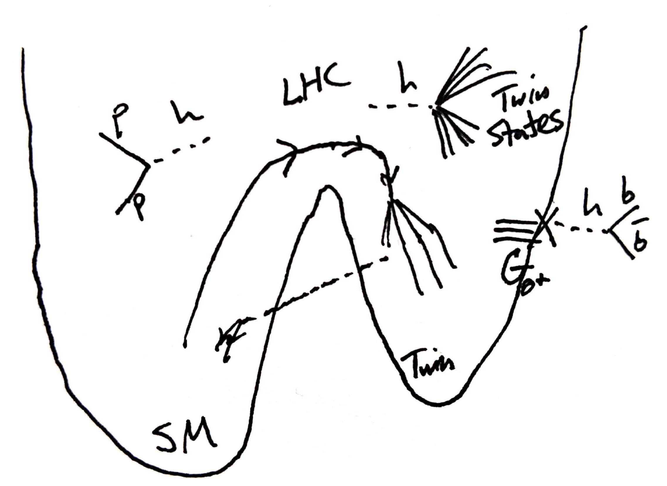
Figure 1: Schematic depiction of hidden valley phenomenology. When another sector is connected to the SM only through heavy particles, it is possible to produce particles from that sector in high energy collisions. If the other sector has phenomenology similar to QCD, this may lead to the production of many states in a dark shower. If (some of) the lowest-lying states in the dark sector may decay back to SM particles, these will generically be displaced decays because they must go through the higher-dimensional operator. In the Twin Higgs, this may be production of either Higgs leading to dark showers with many twin glueballs, some of which mix with the Higgs and decay into SM states. Figure adapted from [436].

In fact there are many reasons an unstable particle may be long-lived, and we see a multitude of examples in the SM itself. In analogy with the hidden valley phenomenology, charged pions are long-lived compared to the QCD scale because their decay must take place through a heavy W boson. Neutrons are similarly very long-lived as a result of their small mass splitting with protons. Protons themselves are very long-lived as a result of an approximate global symmetry (see Section 2 for some little-appreciated subtleties in this reasoning). The SM Higgs is long-lived compared to the electroweak scale because its leading decay mode proceeds through the small bottom quark Yukawas. Given the genericity of long-lived particles in our sector, it’s entirely reasonable to imagine that some dark sector will have similar phenomenology. So even aside from our Neutral Naturalness motivation, such searches are generically useful and interesting things to look for.

In this section we forecast how well an electron-positron collider will be able to probe Higgs decays to long-lived particles, using the parameters for some machines which have been proposed by the community and search strategies of our own design. Such forecasting is crucially important at the present time, as the community is still discussing what the next collider is that we will build. It’s clearly necessary to know what sort of physics program we expect we can carry out before we build a machine to do it. And these studies are used to motivate different types of detectors, their detailed design features and how trigger bandwidth is allocated.

Chapter 6 New Trail for Naturalness

Is commuting dead?

The Connecticut Mirror Headline
June 2, 2020 [478]

Chapter 7 Conclusion

Scientists are baffled: What’s up with the universe?

The Washington Post Headline
November 1, 2019 [590]

We end the way we began: Declaring it to be an exciting time in particle physics. The picture we have painted above on the state of the field is one of uncertainty—and indeed we have barely even touched on many of the important problems of the Standard Model. Dark matter and neutrino masses, while having had canonical, obvious, beautiful solutions in the context of supersymmetric grand unified theories, are also as yet mysterious. These fields have likewise turned their focus toward alternative mechanisms in the past few years as a result of the lack of observational evidence for their standard solutions. But these facts all make the universe a more exciting place to study. Imagine if we had found weak-scale supersymmetry at the LHC, and our job now was simply to interpret the data in terms of which of the supersymmetric extensions proposed and well-studied in the past decades were correct. Or even worse, if technicolor had really been the answer and we had to watch Nature repeat the same trick she used at the strong scale again at the weak scale. How dreadfully boring!

Yes, yes, this attitude is selfish and a bit flippant, but what we now have is the chance to learn more about the universe and about the spectrum of possibilities in physics, and to explore new, radical ideas.

Let me end with a reminder of another, prior era in which theoretical physicists had thought they had everything figured out, recalled by no less than Max Planck in a 1924 talk at the University of Munich, and bring to your mind the outcome of those predictions:

As I began my university studies [in 1878] I asked my venerable teacher Philipp von Jolly for advice regarding the conditions and prospects of my chosen field of study. He described physics to me as a highly developed, nearly fully matured science, that through the crowning achievement of the discovery of the principle of conservation of energy it will arguably soon take its final stable form. It may yet keep going in one corner or another, scrutinizing or putting in order a jot here and a tittle there, but the system as a whole is secured, and theoretical physics is noticeably approaching its completion to the same degree as geometry did centuries ago. That was the view fifty years ago of a respected physicist at the time.
— Max Planck

As translated in Wells (2016) [591] from Planck (1933) [592]

May the universe continue to surprise us. $\square$

Chapter 8 Kinetic Mixing in the Mirror Twin Higgs

Since kinetic mixing plays a central role in freeze-twin dark matter, we discuss here at some length the order at which it is expected in the low-energy EFT. Of course, there may always be UV contributions which set $\epsilon$ to the value needed for freeze-in. However, if the UV completion of the MTH disallows such terms - for example, via supersymmetry, an absence of fields charged under both sectors, and eventually grand unification in each sector (see e.g. [593, 594, 292, 293, 595, 596])- then the natural expectation is for mixing of order these irreducible IR contributions.

To be concrete, we imagine that $\epsilon=0$ at the UV cutoff of the MTH, $\Lambda\lesssim 4\pi f$. To find the kinetic mixing in the regime of relevance, at momenta $\mu\lesssim 1\text{ GeV}$, we must run down to this scale. As we do not have the technology to easily calculate high-loop-order diagrams, our analysis is limited to whether we can prove diagrams at some loop order are vanishing or finite, and so do not generate mixing. Thus our conclusions are strictly always ‘we know no argument that kinetic mixing of this order is not generated’, and there is always the possibility that further hidden cancellations appear. With that caveat divulged, we proceed and consider diagrammatic arguments in both the unbroken and broken phases of electroweak symmetry.

Starting in the unbroken phase, we compute the mixing between the hypercharge gauge bosons. Two- and three-loop diagrams with Higgs loops containing one gauge vertex and one quartic insertion vanish. By charge conjugation in scalar QED, the three-leg amplitude of a gauge boson and a complex scalar pair must be antisymmetric under exchange of the scalars. However, the quartic coupling of the external legs ensures that their momenta enter symmetrically. As this holds off-shell, the presence of a loop which looks like

causes the diagram to vanish. However, at four loops the following diagram can be drawn which avoids this issue:

where the two hypercharges are connected by charged fermion loops in their respective sectors and the Higgs doublets’ quartic interaction. This diagram contributes at least from the MTH cutoff $\Lambda\lesssim 4\pi f$ down to $f$, the scale at which twin and electroweak symmetries are broken. We have no argument that this vanishes nor that its unitarity cuts vanish. We thus expect a contribution to kinetic mixing of $\epsilon\sim g_{1}^{2}c_{W}^{2}/(4\pi)^{8}$, with $g_{1}$ the twin and SM hypercharge coupling and $c_{W}=\cos\theta_{W}$ appearing as the contribution to the photon mixing operator. In this estimate we have omitted any logarithmic dependence on mass scales, as it is subleading.

In the broken phase, we find it easiest to perform this analysis in unitary gauge. The Higgs radial modes now mass-mix, but the emergent charge conjugation symmetries in the two QED sectors allow us to argue vanishing to higher-loop order. The implications of the formal statement of charge conjugation symmetry are subtle because we have two QED sectors, so whether charge conjugation violation is required in both sectors seems unclear. However, similarly to the above case, there is a symmetry argument which holds off-shell. The result we rely on here is that in a vector-like gauge theory, diagrams with any fermion loops with an odd number of gauge bosons cancel pairwise. Thus, each fermion loop must be sensitive to the chiral nature of the theory, so the first non-vanishing contribution is at five loops as in:

where the crosses indicate mass-mixing insertions between the two Higgs radial modes which each contribute $\sim v/f$. Thus, both the running down to low energies and the finite contributions are five-loop suppressed. From such diagrams, one expects a contribution $\epsilon\sim e^{2}g_{A}^{2}g_{V}^{2}(v/f)^{2}/(4\pi)^{10}$, where with $g_{V}$ and $g_{A}$ we denote the vector and axial-vector couplings of the $Z$, respectively. We note there are other five loop diagrams in which Higgses couple to massive vectors which are of similar size or smaller.

Depending on the relative sizes of these contributions, one then naturally expects kinetic mixing of order $\epsilon\sim 10^{-13}-10^{-10}$. If $\epsilon$ is indeed generated at these loop-levels, then mixing on the smaller end of this range likely requires that it becomes disallowed not far above the scale $f$. However, we note that our ability to argue for higher-loop order vanishing in the broken versus unbroken phase is suggestive of the possibility that there may be further cancellations. We note also the possibility that these diagrams, even if nonzero, generate only higher-dimensional operators. Further investigation of the generation of kinetic mixing through a scalar portal is certainly warranted.

Chapter 9 How to Formulate Field Theory on a Noncommutative Space

In this appendix we provide detail on how to formulate field theories on a space which is defined by Equation LABEL:eqn:ncdef, which we repeat here for convenience:

$$\left[\hat{x}^{\mu},\hat{x}^{\nu}\right]=i\theta^{\mu\nu}.$$ (1)

To construct a field theory on this space we must specify the algebra of observables. First we briefly recall the familiar, commutative case. For simplicity, we consider a scalar field theory on flat Euclidean space. We denote by $\text{Alg}\left(\mathbb{R}^{d}[x],\cdot\right)$ the commutative, $C^{*}$-algebra of Schwartz functions of $d$-dimensional Euclidean space with the standard point-wise product, and this constitutes our algebra of observables. A convenient basis for the vector space is that of plane waves $e^{ip\cdot x}$.

The case of interest here is noncommutative flat Euclidean space, on which we define $\text{Alg}\left(\mathbb{R}^{d}_{\theta}[\hat{x}],\cdot\right)$. This now consists of such functions of $d$ variables $\hat{x}^{\mu}$ related by Equation LABEL:eqn:ncdef, and so is a noncommutative algebra, although we’ve specified again the normal ‘point-wise’ product. A useful basis will again be that of plane waves, which we may define as the eigenfunctions of appropriately-defined derivatives on the noncommutative space, and which look familiar $e^{ip\cdot\hat{x}}$. To can get a sense for this algebra it is useful to carry out the simple exercise of multiplying two plane waves by simply applying Baker-Campbell-Hausdorff

$$e^{ik\cdot\hat{x}}\cdot e^{ik^{\prime}\cdot\hat{x}}=\exp\left(ik\cdot\hat{x}+ik^{\prime}\cdot\hat{x}-\frac{1}{2}k_{\mu}k^{\prime}_{\nu}\left[\hat{x}^{\mu},\hat{x}^{\nu}\right]\right)=e^{-\frac{i}{2}\theta^{\mu\nu}k_{\mu}k^{\prime}_{\nu}}e^{i\left(k+k^{\prime}\right)\cdot\hat{x}}.$$ (2)

As in quantum mechanics, we will wish to study noncommutative versions of familiar commutative theories, and so it will be useful to view $\mathbb{R}^{d}_{\theta}$ as a ‘deformation’ of $\mathbb{R}^{d}$. We then wish to construct a map from our commutative algebra to our noncommutative one which returns smoothly to the identity as $\theta^{\mu\nu}\rightarrow 0$. The standard such choice is the Weyl-Wigner map $\hat{\mathcal{W}}$, which one may roughly think of as merely replacing $x$s with $\hat{x}$s.

The procedure is simply to Fourier transform from commutative space to momenta, and then inverse Fourier transform to noncommutative space. Given a commutative space Schwartz function $f$, we may compose the two operations and write

$$\hat{\mathcal{W}}[f]=\int\text{d}^{d}xf(x)\hat{\Delta}(x),\qquad\hat{\Delta}(x)=\int\frac{\text{d}^{d}k}{\left(2\pi\right)^{d}}e^{ik_{i}\cdot\hat{x}^{i}}e^{-ik_{i}\cdot x^{i}}.$$ (3)

Note that this is an injective map of Schwartz functions on $\mathbb{R}^{d}$ to those on $\mathbb{R}^{d}_{\theta}$ which respects the vector space structure but not the structure of the algebra. This property is familiar from quantum mechanics.

We may now construct noncommutative versions of field variables, but we still don’t know how to do physics on these spaces. That is, we can write down the Lagrangian for noncommutative $\phi^{4}$ theory, and we could even determine an action after we formulate a notion of an integral over a noncommutative space. But our familiar results about how to go from the action of a field theory to a calculation for a physical observable most certainly depended implicitly on living on a commutative space, and so it seems we must re-formulate physics from the bottom up.

Fortunately, such a drastic measure may not be necessary, as one may formulate QFT on noncommutative spaces as a simple modification of our normal field theory structure. The core idea is to find an algebra of functions on $\mathbb{R}^{d}$ which is isomorphic to $\text{Alg}\left(\mathbb{R}^{d}_{\theta}[\hat{x}],\cdot\right)$ by pushing the noncommutativity into a new field product, known as a Groenewold-Moyal product (or star-product). We diagram the structure we wish to look for in Figure 1.

Figure 1: The relations between the algebra of a commutative field theory, the noncommutative algebra one finds by applying the Weyl-Wigner map, and the noncommutative algebra most useful for field theory making use of the Groenewold-Moyal product.The vertical arrows respect only the vector space structure, and one should think of constructing a new algebra by applying a vector space map and then endowing the vectors with a multiplication operation.

In particular, we may do this by demanding that our quantization map $\hat{\mathcal{W}}$ is upgraded to an isomorphism between $\text{Alg}\left(\mathbb{R}^{d}_{\theta}[\hat{x}],\cdot\right)$ and an algebra on the vector space of functions of commutative Euclidean space, with a multiplication operation which is chosen to preserve the algebraic structure. That is, we must satisfy

$$\hat{\mathcal{W}}\left[f\star_{\theta}g\right]=\hat{\mathcal{W}}\left[f\right]\cdot\hat{\mathcal{W}}\left[g\right],$$ (4)

for any Schwartz functions $f,g$ on commutative Euclidean space. But we can guarantee this by ensuring it for plane waves, the calculation of which we’ve essentially already done above in Equation 2:

$$e^{ikx}\star_{\theta}e^{ik^{\prime}x} =\hat{\mathcal{W}}^{-1}\left[\hat{\mathcal{W}}\left[e^{ikx}\right]\cdot\hat{\mathcal{W}}\left[e^{ik^{\prime}x}\right]\right]$$

$$=\hat{\mathcal{W}}^{-1}\left[e^{-\frac{i}{2}\theta^{ij}k_{i}k^{\prime}_{j}}e^{i\left(k+k^{\prime}\right)\cdot\hat{x}}\right]$$

$$e^{ikx}\star_{\theta}e^{ik^{\prime}x} \equiv e^{-\frac{i}{2}\theta^{\mu\nu}k_{\mu}k^{\prime}_{\nu}}e^{i\left(k+k^{\prime}\right)\cdot x},$$ (5)

where the $\theta$ subscript merely tells us the star-product will depend on the noncommutativity tensor, and this will henceforth be dropped. This gives a position-space representation of the star-product,

$$f(x)\star g(x)=\left.\exp\left(\frac{i}{2}\theta_{\mu\nu}\partial_{y}^{\mu}\partial_{z}^{\nu}\right)f(y)g(z)\right|_{y=z=x}=f(x)\exp\left(\frac{i}{2}\overleftarrow{\partial}^{\mu}\theta_{\mu\nu}\overrightarrow{\partial}^{\nu}\right)g(x).$$ (6)

The general procedure to construct a noncommutative field theory from a commutative one is then by application of the Weyl-Wigner map. As an example, for a simple $\phi^{n}$ theory we find

$$\mathcal{L}^{(NC)}_{\text{int}}=\frac{\lambda}{n!}\hat{\mathcal{W}}^{-1}\left[\hat{\mathcal{W}}\left(\phi(x)\right)^{n}\right]\ =\frac{\lambda}{n!}\overbrace{\phi(x)\star\phi(x)\star\cdots\star\phi(x)}^{\text{n copies}}.$$ (7)

Chapter 10 Wilsonian Interpretations of NCFTs from Auxiliary Fields

In this appendix we discuss various generalizations of the procedure introduced in [491, 515] to account for the new structures appearing in the noncommutative quantum effective action via the introduction of additional auxiliary fields.

Appendix 10.A Scalar Two-Point Function

It is simple to generalize the procedure discussed in Section LABEL:sec:phi4 to add to the quadratic effective action of $\phi$ any function we wish through judicious choice of the two-point function for an auxiliary field $\sigma$ which linearly mixes with it. In position space, if we wish to add to our effective Lagrangian

$$\Delta\mathcal{L}_{\text{eff}}=\frac{1}{2}c^{2}\phi(x)f(-i\partial)\phi(x),$$ (1)

where $f(-i\partial)$ is any function of momenta, and $c$ is a coupling we’ve taken out for convenience, then we simply add to our tree-level Lagrangian

$$\Delta\mathcal{L}=\frac{1}{2}\sigma(x)f^{-1}(-i\partial)\sigma(x)+ic\sigma(x)\phi(x),$$ (2)

where $f^{-1}$ is the operator inverse of $f$. It should be obvious that this procedure is entirely general. As applied to the Euclidean $\phi^{4}$ model, we may use this procedure to add a second auxiliary field to account for the logarithmic term in the quadratic effective action as

$$\Delta\mathcal{L}=\frac{1}{2}\sigma(x)\frac{1}{\log\left[1-\frac{4}{\Lambda^{2}\partial\circ\partial}\right]}\sigma(x)-\frac{gM}{\sqrt[\ ]{96\pi^{2}}}\sigma(x)\phi(x),$$ (3)

where we point out that the argument of the log is just $4/(\Lambda_{\text{eff}}^{2}p\circ p)$ in position space. We may then try to interpret $\sigma$ also as a new particle. As discussed in [515], its logarithmic propagator may be interpreted as propagation in an additional dimension of spacetime.

Alternatively, we may simply add a single auxiliary field which accounts for both the quadratic and logarithmic IR singularities by formally applying the above procedure. But having assigned them an exotic propagator, it then becomes all the more difficult to interpret such particles as quanta of elementary fields.

Appendix 10.B Fermion Two-Point Function

To account for the IR structure in the fermion two-point function, we must add an auxiliary fermion $\xi$. If we wish to find a contribution to our effective Lagrangian of

$$\Delta\mathcal{L}_{\text{eff}}=c^{2}\bar{\psi}\mathcal{O}\psi,$$ (4)

where $\mathcal{O}$ is any operator on Dirac fields, then we should add to our tree-level Lagrangian

$$\Delta\mathcal{L}=-\bar{\xi}\mathcal{O}^{-1}\xi+c\left(\bar{\xi}\psi+\bar{\psi}\xi\right),$$ (5)

with $\mathcal{O}^{-1}$ the operator inverse of $\mathcal{O}$. In the Lorentzian Yukawa theory of Section LABEL:sec:yukawa, if we add to the Lagrangian

$$\Delta\mathcal{L}=-\overline{\xi}\frac{M-i\not{\partial}/2}{M^{2}-\partial^{2}/4}\left[\log\left(1-\frac{4}{\Lambda^{2}\partial\circ\partial}\right)\right]^{-1}\xi+\frac{g}{2\sqrt[\ ]{2}\pi}\left(\overline{\xi}\psi+\overline{\psi}\xi\right).$$ (6)

we again find a one-loop quadratic effective Lagrangian which is equal to the $\Lambda\rightarrow\infty$ value of the original, but now for any value of $\Lambda$.

Appendix 10.C Three-Point Function

We may further generalize the procedure for introducing auxiliary fields to account for IR poles to the case of poles in the three-point effective action. It’s clear from the form of the IR divergences in Equation LABEL:eqn:3ptfct that they ‘belong’ to each leg, and so naïvely one might think this means that the divergences we’ve already found in the two point functions already fix them. However those corrections only appear in the internal lines and were already proportional to $g^{2}$, and so they will be higher order corrections. Instead we must generate a correction to the vertex function itself which only corrects one of the legs.

To do this we must introduce auxiliary fields connecting each possible partition of the interaction operator. However, while an auxiliary scalar $\chi$ coupled as $\chi\varphi+\chi\overline{\psi}\psi$ would generate a contribution to the vertex which includes the $\chi$ propagator with the $\varphi$ momentum flowing through it, it would also generate a new $(\overline{\psi}\psi)^{2}$ contact operator, which we don’t want. To avoid this we introduce two auxiliary fields with off-diagonal two-point functions, a trick used for similar purposes in [515]. By abandoning minimality, we can essentially use an auxiliary sector to surgically introduce insertions of functions of momenta wherever we want them.

We can first see how this works on the scalar leg. We add to our tree-level Lagrangian

$$\Delta\mathcal{L}=-\chi_{1}(x)f^{-1}(-i\partial)\chi_{2}(x)+\kappa_{1}\chi_{1}(x)\varphi(x)+\kappa_{2}\chi_{2}(x)\star\overline{\psi}(x)\star\psi(x).$$ (7)

Now to integrate out the auxiliary fields we note that for a three point vertex, one may use momentum conservation to put all the noncommutativity between two of the fields. That is, $\chi_{2}(x)\star\overline{\psi}(x)\star\psi(x)=\chi_{2}(x)(\overline{\psi}(x)\star\psi(x))=(\overline{\psi}(x)\star\psi(x))\chi_{2}(x)$ as long as this is not being multiplied by any other functions of $x$. So we may use this form of the interaction to simply integrate out the auxiliary fields. We end up with

$$\Delta\mathcal{L}_{\text{eff}}=\kappa_{1}\kappa_{2}\overline{\psi}\star\psi\star f(-i\partial)\varphi$$ (8)

which is exactly of the right form to account for an IR divergence in the three-point function which only depends on the $\varphi$ momentum.

For the fermionic legs, we need to add fermionic auxiliary fields which split the Yukawa operator in the other possible ways. We introduce Dirac fields $\xi,\xi^{\prime}$ and a differential operator on such fields $\mathcal{O}^{-1}(-i\partial)$. Then if we add to the Lagrangian

$$\Delta\mathcal{L}=-\overline{\xi}\mathcal{O}^{-1}\xi^{\prime}-\overline{\xi^{\prime}}\mathcal{O}^{-1}\xi+c_{1}(\overline{\xi}\star\psi\star\varphi+\overline{\psi}\star\xi\star\varphi)+c_{2}(\overline{\xi}\star\varphi\star\psi+\overline{\psi}\star\varphi\star\xi)+c_{3}(\overline{\xi^{\prime}}\psi+\overline{\psi}\xi^{\prime}),$$ (9)

we now end up with a contribution to the effective Lagrangian

$$\Delta\mathcal{L}_{\text{eff}}=c_{1}c_{3}\left(\bar{\psi}\star\mathcal{O}\left(\psi\right)\star\varphi+\bar{\psi}\star\mathcal{O}\left(\psi\star\varphi\right)\right)+c_{2}c_{3}\left(\bar{\psi}\star\varphi\star\mathcal{O}\left(\psi\right)+\bar{\psi}\star\mathcal{O}\left(\varphi\star\psi\right)\right),$$ (10)

where we have abused notation and now the argument of $\mathcal{O}$ specifies which fields it acts on. These terms have the right form to correct both vertex orderings.

Now that we’ve introduced interactions between auxiliary fields and our original fields, the obvious question to ask is whether we can utilize the same auxiliary fields to correct both the two-point and three-point actions. In fact, using two auxiliary fields with off-diagonal propagators per particle we may insert any corrections we wish. The new trick is to endow the auxiliary field interactions with extra momentum dependence.

For a first example with a scalar, consider differential operators $f$, $\Phi$, and add to the Lagrangian

$$\Delta\mathcal{L}=-\chi_{1}f^{-1}(-i\partial)\chi_{2}+\kappa_{1}\chi_{1}\varphi+\kappa_{2}\chi_{2}\overline{\psi}\star\psi+g\varphi\Phi(-i\partial)\chi_{2}.$$ (11)

We may now integrate out the auxiliary fields and find

$$\Delta\mathcal{L}_{\text{eff}}=g\kappa_{1}\varphi f(\Phi(\varphi))+\kappa_{1}\kappa_{2}\overline{\psi}\star\psi\star f(\varphi)$$ (12)

where we’ve assumed that $f$ and $\Phi$ commute. If we take $\Phi=\mathds{1}$ then we have the interpretation of merely inserting the $\chi$ two-point function in both the two-and three-point functions. But we are also free to use some nontrivial $\Phi$, and thus to make the corrections to the two- and three-point functions have whatever momentum dependence we wish. It should be obvious how to generalize this to insert momentum dependence into the scalar lines of arbitrary $n-$point functions.

The case of a fermion is no more challenging in principle. For differential operators $\mathcal{O},\mathcal{F}$, we add

$$\Delta\mathcal{L}=-\overline{\xi}\mathcal{O}^{-1}\xi^{\prime}-\overline{\xi^{\prime}}\mathcal{O}^{-1}\xi+c_{1}(\overline{\xi}\star\psi\star\varphi+\overline{\psi}\star\xi\star\varphi)+c_{2}(\overline{\xi}\star\varphi\star\psi+\overline{\psi}\star\varphi\star\xi)\\ +c_{3}(\overline{\xi^{\prime}}\psi+\overline{\psi}\xi^{\prime})+\frac{g}{2}\left(\bar{\xi}\mathcal{O}^{-1}\mathcal{F}\psi+\bar{\psi}\mathcal{O}^{-1}\mathcal{F}\xi\right),$$ (13)

and upon integrating out the auxiliary fields we find

$$\Delta\mathcal{L}_{\text{eff}}=gc_{3}\bar{\psi}\mathcal{F}\psi+c_{1}c_{3}\left(\bar{\psi}\star\mathcal{O}\left(\psi\right)\star\varphi+\bar{\psi}\star\mathcal{O}\left(\psi\star\varphi\right)\right)+c_{2}c_{3}\left(\bar{\psi}\star\varphi\star\mathcal{O}\left(\psi\right)+\bar{\psi}\star\mathcal{O}\left(\varphi\star\psi\right)\right),$$ (14)

where the generalization to $n$-points is again clear. Note that in the fermionic case it’s crucial that we be allowed to insert different momentum dependence in the corrections to the two- and three-point functions, as these have different Lorentz structures.

Now we cannot quite implement this for the two- and three-point functions calculated in Section LABEL:sec:yukawa, for the simple reason that we regulated these quantities differently. That is, we have abused notation and the symbol ‘$\Lambda$’ means different things in the results for the two- and three-point functions. In order to carry out this procedure, we could simply regulate the two-point functions in $3d$ Schwinger space, though we run into the technical obstruction that the integration method above only calculates the leading divergence, which is not good enough for the scalar case.

References

- [1] L. Carroll and J. Tenniel, Through the Looking-Glass, and What Alice Found There. Macmillan, 1871.
- [2] T. Cohen, N. Craig, S. Koren, M. McCullough and J. Tooby-Smith, Supersoft Stops, 2002.12630.
- [3] N. Craig and S. Koren, IR Dynamics from UV Divergences: UV/IR Mixing, NCFT, and the Hierarchy Problem, JHEP 03 (2020) 037 [1909.01365].
- [4] S. Koren and R. McGehee, Freezing-in twin dark matter, Phys. Rev. D 101 (2020) 055024 [1908.03559].
- [5] N. Craig, I. Garcia Garcia and S. Koren, The Weak Scale from Weak Gravity, JHEP 09 (2019) 081 [1904.08426].
- [6] S. B. Giddings, S. Koren and G. Treviño, Exploring strong-field deviations from general relativity via gravitational waves, Phys. Rev. D 100 (2019) 044005 [1904.04258].
- [7] S. Koren, Neutrino – Dark Matter Scattering and Coincident Detections of UHE Neutrinos with EM Sources, JCAP 09 (2019) 013 [1903.05096].
- [8] A. Herderschee, S. Koren and T. Trott, Constructing = 4 Coulomb branch superamplitudes, JHEP 08 (2019) 107 [1902.07205].
- [9] A. Herderschee, S. Koren and T. Trott, Massive On-Shell Supersymmetric Scattering Amplitudes, JHEP 10 (2019) 092 [1902.07204].
- [10] S. Alipour-Fard, N. Craig, S. Gori, S. Koren and D. Redigolo, The second Higgs at the lifetime frontier, JHEP 07 (2020) 029 [1812.09315].
- [11] N. Craig, I. Garcia Garcia and S. Koren, Discrete Gauge Symmetries and the Weak Gravity Conjecture, JHEP 05 (2019) 140 [1812.08181].
- [12] S. Alipour-Fard, N. Craig, M. Jiang and S. Koren, Long Live the Higgs Factory: Higgs Decays to Long-Lived Particles at Future Lepton Colliders, Chin. Phys. C 43 (2019) 053101 [1812.05588].
- [13] N. Craig, S. Koren and T. Trott, Cosmological Signals of a Mirror Twin Higgs, JHEP 05 (2017) 038 [1611.07977].
- [14] S. C. Koren, C. H. Blake, C. C. Dahn and H. C. Harris, The Low-mass Astrometric Binary LSR 1610-0040, The Astronomical Journal 151 (2016) 57 [1511.02234].
- [15] S. C. Koren, E. L. Wright and A. Mainzer, Characterizing asteroids multiply-observed at infrared wavelengths, Icarus 258 (2015) 82 [1506.04751].
- [16] T. Cohen, As Scales Become Separated: Lectures on Effective Field Theory, PoS TASI2018 (2019) 011 [1903.03622].
- [17] H. Georgi, Effective field theory, Ann. Rev. Nucl. Part. Sci. 43 (1993) 209.
- [18] M. Srednicki, Quantum field theory. Cambridge University Press, 2007.
- [19] M. E. Peskin and D. V. Schroeder, An Introduction to quantum field theory. Addison-Wesley, Reading, USA, 1995.
- [20] A. Zee, Quantum field theory in a nutshell. 11, 2003.
- [21] J. Polchinski, Renormalization and Effective Lagrangians, Nucl. Phys. B 231 (1984) 269.
- [22] M. D. Schwartz, Quantum Field Theory and the Standard Model. Cambridge University Press, 3, 2014.
- [23] J. P. Society, The Jewish Bible Tanakhh: The New Jps Translation According to the Traditional Hebrew Text. Jewish Publication Society, 2007.
- [24] P. W. Anderson, Plasmons, Gauge Invariance, and Mass, Phys. Rev. 130 (1963) 439.
- [25] F. Englert and R. Brout, Broken Symmetry and the Mass of Gauge Vector Mesons, Phys. Rev. Lett. 13 (1964) 321.
- [26] G. Guralnik, C. Hagen and T. Kibble, Global Conservation Laws and Massless Particles, Phys. Rev. Lett. 13 (1964) 585.
- [27] P. W. Higgs, Broken symmetries, massless particles and gauge fields, Phys. Lett. 12 (1964) 132.
- [28] P. W. Higgs, Broken Symmetries and the Masses of Gauge Bosons, Phys. Rev. Lett. 13 (1964) 508.
- [29] G. ’t Hooft, Renormalizable Lagrangians for Massive Yang-Mills Fields, Nucl. Phys. B 35 (1971) 167.
- [30] P. Langacker, The standard model and beyond. 2, 2010.
- [31] C. Burgess and G. Moore, The standard model: A primer. Cambridge University Press, 12, 2006.
- [32] B. Grzadkowski, M. Iskrzynski, M. Misiak and J. Rosiek, Dimension-Six Terms in the Standard Model Lagrangian, JHEP 10 (2010) 085 [1008.4884].
- [33] B. Gripaios and D. Sutherland, DEFT: A program for operators in EFT, JHEP 01 (2019) 128 [1807.07546].
- [34] J. de Blas, J. Criado, M. Perez-Victoria and J. Santiago, Effective description of general extensions of the Standard Model: the complete tree-level dictionary, JHEP 03 (2018) 109 [1711.10391].
- [35] I. Brivio, Y. Jiang and M. Trott, The SMEFTsim package, theory and tools, JHEP 12 (2017) 070 [1709.06492].
- [36] A. Falkowski, M. González-Alonso and K. Mimouni, Compilation of low-energy constraints on 4-fermion operators in the SMEFT, JHEP 08 (2017) 123 [1706.03783].
- [37] J. Ellis, C. W. Murphy, V. Sanz and T. You, Updated Global SMEFT Fit to Higgs, Diboson and Electroweak Data, JHEP 06 (2018) 146 [1803.03252].
- [38] J. de Blas, M. Ciuchini, E. Franco, S. Mishima, M. Pierini, L. Reina et al., The Global Electroweak and Higgs Fits in the LHC era, PoS EPS-HEP2017 (2017) 467 [1710.05402].
- [39] I. Brivio and M. Trott, The Standard Model as an Effective Field Theory, Phys. Rept. 793 (2019) 1 [1706.08945].
- [40] E. Fermi, An attempt of a theory of beta radiation. 1., Z. Phys. 88 (1934) 161.
- [41] J. C. Pati and A. Salam, Lepton Number as the Fourth Color, Phys. Rev. D 10 (1974) 275.
- [42] H. Georgi and S. Glashow, Unity of All Elementary Particle Forces, Phys. Rev. Lett. 32 (1974) 438.
- [43] A. Einstein, Considerations concerning the fundaments of theoretical physics, Science 91 (1940) 487 [https://science.sciencemag.org/content/91/2369/487.full.pdf].
- [44] C. Kounnas, A. Masiero, D. V. Nanopoulos and K. A. Olive, Grand Unification With and Without Supersymmetry and Cosmological Implications. 1985.
- [45] G. G. Ross, Grand Unified Theories. 1985.
- [46] S. Raby, Supersymmetric Grand Unified Theories: From Quarks to Strings via SUSY GUTs, vol. 939. Springer, 2017, 10.1007/978-3-319-55255-2.
- [47] M. Sher, Grand unification, Higgs bosons, and baryogenesis, in Strings, Branes and Extra Dimensions: TASI 2001: Proceedings, 2001.
- [48] Particle Data Group collaboration, Review of Particle Physics, Phys. Rev. D98 (2018) 030001.
- [49] S. Coleman, Aspects of Symmetry: Selected Erice Lectures. Cambridge University Press, Cambridge, U.K., 1985, 10.1017/CBO9780511565045.
- [50] R. A. Bertlmann, Anomalies in quantum field theory, vol. 91. Oxford University Press, 2000.
- [51] R. Rajaraman, Solitons and Instantons: An Introduction to Solitons and Instantons in Quantum Field Theory, North-Holland personal library. North-Holland Publishing Company, 1982.
- [52] S. Hawking, The Unpredictability of Quantum Gravity, Commun. Math. Phys. 87 (1982) 395.
- [53] T. Banks, L. Susskind and M. E. Peskin, Difficulties for the Evolution of Pure States Into Mixed States, Nucl. Phys. B 244 (1984) 125.
- [54] A. B. Goncharov, A simple construction of Grassmannian polylogarithms, arXiv e-prints (2009) arXiv:0908.2238 [0908.2238].
- [55] A. B. Goncharov, M. Spradlin, C. Vergu and A. Volovich, Classical Polylogarithms for Amplitudes and Wilson Loops, Phys. Rev. Lett. 105 (2010) 151605 [1006.5703].
- [56] C. Duhr, H. Gangl and J. R. Rhodes, From polygons and symbols to polylogarithmic functions, JHEP 10 (2012) 075 [1110.0458].
- [57] D. Gaiotto, J. Maldacena, A. Sever and P. Vieira, Pulling the straps of polygons, JHEP 12 (2011) 011 [1102.0062].
- [58] C. Duhr, Mathematical aspects of scattering amplitudes, in Theoretical Advanced Study Institute in Elementary Particle Physics: Journeys Through the Precision Frontier: Amplitudes for Colliders, pp. 419–476, 2015, DOI [1411.7538].
- [59] N. Arkani-Hamed, J. L. Bourjaily, F. Cachazo, A. B. Goncharov, A. Postnikov and J. Trnka, Grassmannian Geometry of Scattering Amplitudes. Cambridge University Press, 4, 2016, 10.1017/CBO9781316091548, [1212.5605].
- [60] S. Mandelstam, Determination of the pion - nucleon scattering amplitude from dispersion relations and unitarity. General theory, Phys. Rev. 112 (1958) 1344.
- [61] K. G. Wilson, The Renormalization Group: Critical Phenomena and the Kondo Problem, Rev. Mod. Phys. 47 (1975) 773.
- [62] T. Appelquist and J. Carazzone, Infrared Singularities and Massive Fields, Phys. Rev. D 11 (1975) 2856.
- [63] B. Delamotte, A Hint of renormalization, Am. J. Phys. 72 (2004) 170 [hep-th/0212049].
- [64] A. Neumaier, Renormalization without infinities – an elementary tutorial, Jun, 2015.
- [65] S. Weinberg, The Quantum theory of fields. Vol. 1: Foundations. Cambridge University Press, 6, 2005.
- [66] T. Schäfer and E. V. Shuryak, Instantons in QCD, Rev. Mod. Phys. 70 (1998) 323 [hep-ph/9610451].
- [67] S. Vandoren and P. van Nieuwenhuizen, Lectures on instantons, 0802.1862.
- [68] G. V. Dunne and M. Unsal, Resurgence and Trans-series in Quantum Field Theory: The CP(N-1) Model, JHEP 11 (2012) 170 [1210.2423].
- [69] G. V. Dunne and M. Unsal, Uniform WKB, Multi-instantons, and Resurgent Trans-Series, Phys. Rev. D 89 (2014) 105009 [1401.5202].
- [70] D. Dorigoni, An Introduction to Resurgence, Trans-Series and Alien Calculus, Annals Phys. 409 (2019) 167914 [1411.3585].
- [71] M. Mariño, Instantons and Large N: An Introduction to Non-Perturbative Methods in Quantum Field Theory. Cambridge University Press, 9, 2015.
- [72] J. C. Collins, Renormalization, vol. 26 of Cambridge Monographs on Mathematical Physics. Cambridge University Press, Cambridge, 1986.
- [73] D. Skinner, “The renormalization group.”
- [74] S. R. Coleman and J. Mandula, All Possible Symmetries of the S Matrix, Phys. Rev. 159 (1967) 1251.
- [75] J. Polchinski, Scale and Conformal Invariance in Quantum Field Theory, Nucl. Phys. B 303 (1988) 226.
- [76] Y. Nakayama, Scale invariance vs conformal invariance, Phys. Rept. 569 (2015) 1 [1302.0884].
- [77] D. J. Gross and F. Wilczek, Ultraviolet Behavior of Nonabelian Gauge Theories, Phys. Rev. Lett. 30 (1973) 1343.
- [78] H. Politzer, Reliable Perturbative Results for Strong Interactions?, Phys. Rev. Lett. 30 (1973) 1346.
- [79] Manuscripts 78-81, in Collected Papers of L.D. Landau, D. T. HAAR], ed., pp. 607 – 610, Pergamon, (1965), DOI.
- [80] K. von Meyenn, Über das relativitätsprinzip und die aus demselben gezogenen folgerungen, in Albert Einsteins Relativitätstheorie: Die grundlegenden Arbeiten, K. von Meyenn, ed., (Wiesbaden), pp. 160–214, Vieweg+Teubner Verlag, (1990), DOI.
- [81] S. Weinberg, Photons and Gravitons in -Matrix Theory: Derivation of Charge Conservation and Equality of Gravitational and Inertial Mass, Phys. Rev. 135 (1964) B1049.
- [82] P. A. Dirac, New basis for cosmology, Proc. Roy. Soc. Lond. A A165 (1938) 199.
- [83] G. ’t Hooft, Naturalness, chiral symmetry, and spontaneous chiral symmetry breaking, NATO Sci. Ser. B 59 (1980) 135.
- [84] K. Zhou, Cosmological relaxation, 2019.
- [85] G. D’Ambrosio, G. Giudice, G. Isidori and A. Strumia, Minimal flavor violation: An Effective field theory approach, Nucl. Phys. B 645 (2002) 155 [hep-ph/0207036].
- [86] Y. Grossman and P. Tanedo, Just a Taste: Lectures on Flavor Physics, in Theoretical Advanced Study Institute in Elementary Particle Physics: Anticipating the Next Discoveries in Particle Physics, pp. 109–295, 2018, DOI [1711.03624].
- [87] J. Zupan, Introduction to flavour physics, CERN Yellow Rep. School Proc. 6 (2019) 181 [1903.05062].
- [88] S. Gori, TASI lectures on flavor physics, PoS TASI2018 (2019) 013.
- [89] N. Arkani-Hamed, The Future of Fundamental Physics, Daedalus 141 (2012) 53.
- [90] S. Samuel, The Standard model in its other phase, Nucl. Phys. B 597 (2001) 70 [hep-ph/9910559].
- [91] C. Quigg and R. Shrock, Gedanken Worlds without Higgs: QCD-Induced Electroweak Symmetry Breaking, Phys. Rev. D 79 (2009) 096002 [0901.3958].
- [92] B. R. Holstein and J. F. Donoghue, Classical physics and quantum loops, Phys. Rev. Lett. 93 (2004) 201602 [hep-th/0405239].
- [93] G. W. Anderson and D. J. Castano, Measures of fine tuning, Phys. Lett. B 347 (1995) 300 [hep-ph/9409419].
- [94] S. Fichet, Quantified naturalness from Bayesian statistics, Phys. Rev. D 86 (2012) 125029 [1204.4940].
- [95] R. Barbieri and G. F. Giudice, Upper Bounds on Supersymmetric Particle Masses, Nucl. Phys. B306 (1988) 63.
- [96] P. Athron and D. Miller, A New Measure of Fine Tuning, Phys. Rev. D 76 (2007) 075010 [0705.2241].
- [97] C. Cheung and G. N. Remmen, Naturalness and the Weak Gravity Conjecture, Phys. Rev. Lett. 113 (2014) 051601 [1402.2287].
- [98] H. Ooguri and C. Vafa, Non-supersymmetric AdS and the Swampland, Adv. Theor. Math. Phys. 21 (2017) 1787 [1610.01533].
- [99] L. E. Ibanez, V. Martin-Lozano and I. Valenzuela, Constraining Neutrino Masses, the Cosmological Constant and BSM Physics from the Weak Gravity Conjecture, JHEP 11 (2017) 066 [1706.05392].
- [100] L. E. Ibanez, V. Martin-Lozano and I. Valenzuela, Constraining the EW Hierarchy from the Weak Gravity Conjecture, 1707.05811.
- [101] Y. Hamada and G. Shiu, Weak Gravity Conjecture, Multiple Point Principle and the Standard Model Landscape, JHEP 11 (2017) 043 [1707.06326].
- [102] D. Lust and E. Palti, Scalar Fields, Hierarchical UV/IR Mixing and The Weak Gravity Conjecture, JHEP 02 (2018) 040 [1709.01790].
- [103] E. Gonzalo, A. Herráez and L. E. Ibáñez, AdS-phobia, the WGC, the Standard Model and Supersymmetry, JHEP 06 (2018) 051 [1803.08455].
- [104] E. Gonzalo and L. E. Ibáñez, The Fundamental Need for a SM Higgs and the Weak Gravity Conjecture, Phys. Lett. B786 (2018) 272 [1806.09647].
- [105] J. March-Russell and R. Petrossian-Byrne, QCD, Flavor, and the de Sitter Swampland, 2006.01144.
- [106] G. Box, Robustness in the strategy of scientific model building, in Robustness in Statistics, R. L. LAUNER and G. N. WILKINSON, eds., pp. 201 – 236, Academic Press, (1979), DOI.
- [107] A. de Gouvea, D. Hernandez and T. M. P. Tait, Criteria for Natural Hierarchies, Phys. Rev. D 89 (2014) 115005 [1402.2658].
- [108] G. Harrison, The inner light, 1968.
- [109] M. Sendak and S. Inc, Chicken Soup with Rice: A Book of Months. Scholastic Incorporated, 1962.
- [110] R. Haag, J. T. Lopuszanski and M. Sohnius, All Possible Generators of Supersymmetries of the s Matrix, Nucl. Phys. B 88 (1975) 257.
- [111] J. Terning, Modern supersymmetry: Dynamics and duality. 4, 2006, 10.1093/acprof:oso/9780198567639.001.0001.
- [112] S. P. Martin, A Supersymmetry primer, in Perspectives on supersymmetry. Vol.2, G. L. Kane, ed., vol. 21, pp. 1–153, (2010), hep-ph/9709356, DOI.
- [113] D. Shih, Supersymmetry, Jan, 2014.
- [114] D. Bertolini, J. Thaler and Z. Thomas, Super-Tricks for Superspace, in Theoretical Advanced Study Institute in Elementary Particle Physics: Searching for New Physics at Small and Large Scales, pp. 421–496, 2013, DOI [1302.6229].
- [115] V. Nair, A Current Algebra for Some Gauge Theory Amplitudes, Phys. Lett. B 214 (1988) 215.
- [116] N. Arkani-Hamed, F. Cachazo and J. Kaplan, What is the Simplest Quantum Field Theory?, JHEP 09 (2010) 016 [0808.1446].
- [117] H. Elvang and Y.-t. Huang, Scattering Amplitudes in Gauge Theory and Gravity. Cambridge University Press, 4, 2015.
- [118] N. Arkani-Hamed, T.-C. Huang and Y.-t. Huang, Scattering Amplitudes For All Masses and Spins, 1709.04891.
- [119] H. K. Dreiner, H. E. Haber and S. P. Martin, Two-component spinor techniques and Feynman rules for quantum field theory and supersymmetry, Phys. Rept. 494 (2010) 1 [0812.1594].
- [120] S. Dimopoulos and H. Georgi, Softly Broken Supersymmetry and SU(5), Nucl. Phys. B 193 (1981) 150.
- [121] R. Davies, J. March-Russell and M. McCullough, A Supersymmetric One Higgs Doublet Model, JHEP 04 (2011) 108 [1103.1647].
- [122] D. Chung, L. Everett, G. Kane, S. King, J. D. Lykken and L.-T. Wang, The Soft supersymmetry breaking Lagrangian: Theory and applications, Phys. Rept. 407 (2005) 1 [hep-ph/0312378].
- [123] A. H. Chamseddine, R. L. Arnowitt and P. Nath, Locally Supersymmetric Grand Unification, Phys. Rev. Lett. 49 (1982) 970.
- [124] R. Barbieri, S. Ferrara and C. A. Savoy, Gauge Models with Spontaneously Broken Local Supersymmetry, Phys. Lett. B 119 (1982) 343.
- [125] L. E. Ibanez, Locally Supersymmetric SU(5) Grand Unification, Phys. Lett. B 118 (1982) 73.
- [126] L. J. Hall, J. D. Lykken and S. Weinberg, Supergravity as the Messenger of Supersymmetry Breaking, Phys. Rev. D 27 (1983) 2359.
- [127] N. Ohta, GRAND UNIFIED THEORIES BASED ON LOCAL SUPERSYMMETRY, Prog. Theor. Phys. 70 (1983) 542.
- [128] J. R. Ellis, D. V. Nanopoulos and K. Tamvakis, Grand Unification in Simple Supergravity, Phys. Lett. B 121 (1983) 123.
- [129] L. Alvarez-Gaume, J. Polchinski and M. B. Wise, Minimal Low-Energy Supergravity, Nucl. Phys. B 221 (1983) 495.
- [130] M. Dine and W. Fischler, A Phenomenological Model of Particle Physics Based on Supersymmetry, Phys. Lett. B 110 (1982) 227.
- [131] C. R. Nappi and B. A. Ovrut, Supersymmetric Extension of the SU(3) x SU(2) x U(1) Model, Phys. Lett. B 113 (1982) 175.
- [132] L. Alvarez-Gaume, M. Claudson and M. B. Wise, Low-Energy Supersymmetry, Nucl. Phys. B 207 (1982) 96.
- [133] M. Dine and A. E. Nelson, Dynamical supersymmetry breaking at low-energies, Phys. Rev. D 48 (1993) 1277 [hep-ph/9303230].
- [134] M. Dine, A. E. Nelson and Y. Shirman, Low-energy dynamical supersymmetry breaking simplified, Phys. Rev. D 51 (1995) 1362 [hep-ph/9408384].
- [135] M. Dine, A. E. Nelson, Y. Nir and Y. Shirman, New tools for low-energy dynamical supersymmetry breaking, Phys. Rev. D 53 (1996) 2658 [hep-ph/9507378].
- [136] E. A. Mirabelli and M. E. Peskin, Transmission of supersymmetry breaking from a four-dimensional boundary, Phys. Rev. D 58 (1998) 065002 [hep-th/9712214].
- [137] D. Kaplan, G. D. Kribs and M. Schmaltz, Supersymmetry breaking through transparent extra dimensions, Phys. Rev. D 62 (2000) 035010 [hep-ph/9911293].
- [138] Z. Chacko, M. A. Luty, A. E. Nelson and E. Ponton, Gaugino mediated supersymmetry breaking, JHEP 01 (2000) 003 [hep-ph/9911323].
- [139] M. Schmaltz and W. Skiba, The Superpartner spectrum of gaugino mediation, Phys. Rev. D 62 (2000) 095004 [hep-ph/0004210].
- [140] M. Schmaltz and W. Skiba, Minimal gaugino mediation, Phys. Rev. D 62 (2000) 095005 [hep-ph/0001172].
- [141] C. Csaki, J. Erlich, C. Grojean and G. D. Kribs, 4-D constructions of supersymmetric extra dimensions and gaugino mediation, Phys. Rev. D 65 (2002) 015003 [hep-ph/0106044].
- [142] H. Cheng, D. Kaplan, M. Schmaltz and W. Skiba, Deconstructing Gaugino Mediation, Phys. Lett. B 515 (2001) 395 [hep-ph/0106098].
- [143] L. Randall and R. Sundrum, Out of this world supersymmetry breaking, Nucl. Phys. B 557 (1999) 79 [hep-th/9810155].
- [144] G. F. Giudice, R. Rattazzi and J. D. Wells, Quantum gravity and extra dimensions at high-energy colliders, Nucl. Phys. B 544 (1999) 3 [hep-ph/9811291].
- [145] J. A. Bagger, T. Moroi and E. Poppitz, Anomaly mediation in supergravity theories, JHEP 04 (2000) 009 [hep-th/9911029].
- [146] K. A. Intriligator and N. Seiberg, Lectures on Supersymmetry Breaking, Class. Quant. Grav. 24 (2007) S741 [hep-ph/0702069].
- [147] E. Witten, Dynamical Breaking of Supersymmetry, Nucl. Phys. B 188 (1981) 513.
- [148] I. Affleck, M. Dine and N. Seiberg, Dynamical Supersymmetry Breaking in Supersymmetric QCD, Nucl. Phys. B 241 (1984) 493.
- [149] I. Affleck, M. Dine and N. Seiberg, Supersymmetry Breaking by Instantons, Phys. Rev. Lett. 51 (1983) 1026.
- [150] I. Affleck, M. Dine and N. Seiberg, Calculable Nonperturbative Supersymmetry Breaking, Phys. Rev. Lett. 52 (1984) 1677.
- [151] I. Affleck, M. Dine and N. Seiberg, Dynamical Supersymmetry Breaking in Four-Dimensions and Its Phenomenological Implications, Nucl. Phys. B 256 (1985) 557.
- [152] N. Seiberg, Exact results on the space of vacua of four-dimensional SUSY gauge theories, Phys. Rev. D 49 (1994) 6857 [hep-th/9402044].
- [153] K. A. Intriligator and N. Seiberg, Lectures on supersymmetric gauge theories and electric-magnetic duality, Subnucl. Ser. 34 (1997) 237 [hep-th/9509066].
- [154] M. A. Shifman, Nonperturbative dynamics in supersymmetric gauge theories, Prog. Part. Nucl. Phys. 39 (1997) 1 [hep-th/9704114].
- [155] M. E. Peskin, Duality in supersymmetric Yang-Mills theory, in Theoretical Advanced Study Institute in Elementary Particle Physics (TASI 96): Fields, Strings, and Duality, pp. 729–809, 2, 1997, hep-th/9702094.
- [156] E. Poppitz and S. P. Trivedi, Dynamical supersymmetry breaking, Ann. Rev. Nucl. Part. Sci. 48 (1998) 307 [hep-th/9803107].
- [157] K. A. Intriligator, N. Seiberg and D. Shih, Dynamical SUSY breaking in meta-stable vacua, JHEP 04 (2006) 021 [hep-th/0602239].
- [158] M. Shifman, Advanced topics in quantum field theory.: A lecture course. Cambridge Univ. Press, Cambridge, UK, 2, 2012.
- [159] M. J. Strassler, An Unorthodox introduction to supersymmetric gauge theory, in Theoretical Advanced Study Institute in Elementary Particle Physics (TASI 2001): Strings, Branes and EXTRA Dimensions, pp. 561–638, 9, 2003, DOI [hep-th/0309149].
- [160] A. E. Nelson and N. Seiberg, R symmetry breaking versus supersymmetry breaking, Nucl. Phys. B 416 (1994) 46 [hep-ph/9309299].
- [161] M. A. Vasiliev, Consistent equation for interacting gauge fields of all spins in (3+1)-dimensions, Phys. Lett. B 243 (1990) 378.
- [162] J. Wess and J. Bagger, Supersymmetry and supergravity. Princeton University Press, Princeton, NJ, USA, 1992.
- [163] D. Z. Freedman and A. Van Proeyen, Supergravity. Cambridge Univ. Press, Cambridge, UK, 5, 2012.
- [164] E. Abbott, Flatland: A Romance of Many Dimensions. Roberts Brothers, 1885.
- [165] G. Nordstrom, On the possibility of unifying the electromagnetic and the gravitational fields, Phys. Z. 15 (1914) 504 [physics/0702221].
- [166] T. Kaluza, Zum Unitätsproblem der Physik, Int. J. Mod. Phys. D 27 (2018) 1870001 [1803.08616].
- [167] O. Klein, Quantum Theory and Five-Dimensional Theory of Relativity. (In German and English), Z. Phys. 37 (1926) 895.
- [168] N. Arkani-Hamed, S. Dimopoulos and G. Dvali, The Hierarchy problem and new dimensions at a millimeter, Phys. Lett. B 429 (1998) 263 [hep-ph/9803315].
- [169] C. Hoyle, U. Schmidt, B. R. Heckel, E. Adelberger, J. Gundlach, D. Kapner et al., Submillimeter tests of the gravitational inverse square law: a search for ’large’ extra dimensions, Phys. Rev. Lett. 86 (2001) 1418 [hep-ph/0011014].
- [170] E. Adelberger, J. Gundlach, B. Heckel, S. Hoedl and S. Schlamminger, Torsion balance experiments: A low-energy frontier of particle physics, Prog. Part. Nucl. Phys. 62 (2009) 102.
- [171] J. Lee, E. Adelberger, T. Cook, S. Fleischer and B. Heckel, New Test of the Gravitational Law at Separations down to 52 m, Phys. Rev. Lett. 124 (2020) 101101 [2002.11761].
- [172] J. Polchinski, S. Chaudhuri and C. V. Johnson, Notes on D-branes, hep-th/9602052.
- [173] J. Polchinski, Tasi lectures on D-branes, in Theoretical Advanced Study Institute in Elementary Particle Physics (TASI 96): Fields, Strings, and Duality, pp. 293–356, 11, 1996, hep-th/9611050.
- [174] C. V. Johnson, D-brane primer, in Theoretical Advanced Study Institute in Elementary Particle Physics (TASI 99): Strings, Branes, and Gravity, pp. 129–350, 7, 2000, DOI [hep-th/0007170].
- [175] I. Antoniadis, N. Arkani-Hamed, S. Dimopoulos and G. Dvali, New dimensions at a millimeter to a Fermi and superstrings at a TeV, Phys. Lett. B 436 (1998) 257 [hep-ph/9804398].
- [176] G. Shiu and S. Tye, TeV scale superstring and extra dimensions, Phys. Rev. D 58 (1998) 106007 [hep-th/9805157].
- [177] L. E. Ibanez, F. Marchesano and R. Rabadan, Getting just the standard model at intersecting branes, JHEP 11 (2001) 002 [hep-th/0105155].
- [178] N. Arkani-Hamed, S. Dimopoulos and G. Dvali, Phenomenology, astrophysics and cosmology of theories with submillimeter dimensions and TeV scale quantum gravity, Phys. Rev. D 59 (1999) 086004 [hep-ph/9807344].
- [179] T. G. Rizzo and J. D. Wells, Electroweak precision measurements and collider probes of the standard model with large extra dimensions, Phys. Rev. D 61 (2000) 016007 [hep-ph/9906234].
- [180] S. Cullen and M. Perelstein, SN1987A constraints on large compact dimensions, Phys. Rev. Lett. 83 (1999) 268 [hep-ph/9903422].
- [181] K. R. Dienes, E. Dudas and T. Gherghetta, Grand unification at intermediate mass scales through extra dimensions, Nucl. Phys. B 537 (1999) 47 [hep-ph/9806292].
- [182] K. R. Dienes, E. Dudas and T. Gherghetta, Extra space-time dimensions and unification, Phys. Lett. B 436 (1998) 55 [hep-ph/9803466].
- [183] N. Arkani-Hamed and M. Schmaltz, Hierarchies without symmetries from extra dimensions, Phys. Rev. D 61 (2000) 033005 [hep-ph/9903417].
- [184] J. L. Hewett, Indirect collider signals for extra dimensions, Phys. Rev. Lett. 82 (1999) 4765 [hep-ph/9811356].
- [185] P. C. Argyres, S. Dimopoulos and J. March-Russell, Black holes and submillimeter dimensions, Phys. Lett. B 441 (1998) 96 [hep-th/9808138].
- [186] R. Emparan, G. T. Horowitz and R. C. Myers, Black holes radiate mainly on the brane, Phys. Rev. Lett. 85 (2000) 499 [hep-th/0003118].
- [187] S. B. Giddings and S. D. Thomas, High-energy colliders as black hole factories: The End of short distance physics, Phys. Rev. D 65 (2002) 056010 [hep-ph/0106219].
- [188] D. M. Eardley and S. B. Giddings, Classical black hole production in high-energy collisions, Phys. Rev. D 66 (2002) 044011 [gr-qc/0201034].
- [189] V. Rubakov, Large and infinite extra dimensions: An Introduction, Phys. Usp. 44 (2001) 871 [hep-ph/0104152].
- [190] R. Maartens and K. Koyama, Brane-World Gravity, Living Rev. Rel. 13 (2010) 5 [1004.3962].
- [191] C. Csaki, TASI lectures on extra dimensions and branes, in Theoretical Advanced Study Institute in Elementary Particle Physics (TASI 2002): Particle Physics and Cosmology: The Quest for Physics Beyond the Standard Model(s), pp. 605–698, 4, 2004, hep-ph/0404096.
- [192] G. D. Kribs, TASI 2004 lectures on the phenomenology of extra dimensions, in Theoretical Advanced Study Institute in Elementary Particle Physics: Physics in D 4, pp. 633–699, 5, 2006, hep-ph/0605325.
- [193] A. Perez-Lorenzana, An Introduction to extra dimensions, J. Phys. Conf. Ser. 18 (2005) 224 [hep-ph/0503177].
- [194] H.-C. Cheng, Introduction to Extra Dimensions, in Theoretical Advanced Study Institute in Elementary Particle Physics: Physics of the Large and the Small, pp. 125–162, 2011, DOI [1003.1162].
- [195] C. Csaki, J. Hubisz and P. Meade, TASI lectures on electroweak symmetry breaking from extra dimensions, in Theoretical Advanced Study Institute in Elementary Particle Physics: Physics in D 4, pp. 703–776, 10, 2005, hep-ph/0510275.
- [196] M. Quiros, New ideas in symmetry breaking, in Theoretical Advanced Study Institute in Elementary Particle Physics (TASI 2002): Particle Physics and Cosmology: The Quest for Physics Beyond the Standard Model(s), pp. 549–601, 2, 2003, hep-ph/0302189.
- [197] A. Delgado, A. Pomarol and M. Quiros, Supersymmetry and electroweak breaking from extra dimensions at the TeV scale, Phys. Rev. D 60 (1999) 095008 [hep-ph/9812489].
- [198] R. Barbieri, L. J. Hall and Y. Nomura, Models of Scherk-Schwarz symmetry breaking in 5-D: Classification and calculability, Nucl. Phys. B 624 (2002) 63 [hep-th/0107004].
- [199] L. J. Hall and Y. Nomura, Gauge unification in higher dimensions, Phys. Rev. D 64 (2001) 055003 [hep-ph/0103125].
- [200] J. Scherk and J. H. Schwarz, Spontaneous Breaking of Supersymmetry Through Dimensional Reduction, Phys. Lett. B 82 (1979) 60.
- [201] J. Scherk and J. H. Schwarz, How to Get Masses from Extra Dimensions, Nucl. Phys. B 153 (1979) 61.
- [202] I. Antoniadis and K. Benakli, Limits on extra dimensions in orbifold compactifications of superstrings, Phys. Lett. B 326 (1994) 69 [hep-th/9310151].
- [203] I. Antoniadis, S. Dimopoulos, A. Pomarol and M. Quiros, Soft masses in theories with supersymmetry breaking by TeV compactification, Nucl. Phys. B 544 (1999) 503 [hep-ph/9810410].
- [204] A. Pomarol and M. Quiros, The Standard model from extra dimensions, Phys. Lett. B 438 (1998) 255 [hep-ph/9806263].
- [205] R. Barbieri, L. J. Hall and Y. Nomura, A Constrained standard model from a compact extra dimension, Phys. Rev. D 63 (2001) 105007 [hep-ph/0011311].
- [206] R. Barbieri, L. J. Hall and Y. Nomura, Softly broken supersymmetric desert from orbifold compactification, Phys. Rev. D 66 (2002) 045025 [hep-ph/0106190].
- [207] L. J. Hall, Y. Nomura and D. Tucker-Smith, Gauge Higgs unification in higher dimensions, Nucl. Phys. B 639 (2002) 307 [hep-ph/0107331].
- [208] N. Haba, Y. Hosotani, Y. Kawamura and T. Yamashita, Dynamical symmetry breaking in gauge Higgs unification on orbifold, Phys. Rev. D 70 (2004) 015010 [hep-ph/0401183].
- [209] C. Lim and N. Maru, Towards a realistic grand gauge-Higgs unification, Phys. Lett. B 653 (2007) 320 [0706.1397].
- [210] A. Furui, Y. Hosotani and N. Yamatsu, Toward Realistic Gauge-Higgs Grand Unification, PTEP 2016 (2016) 093B01 [1606.07222].
- [211] N. Manton, A New Six-Dimensional Approach to the Weinberg-Salam Model, Nucl. Phys. B 158 (1979) 141.
- [212] P. Forgacs and N. Manton, Space-Time Symmetries in Gauge Theories, Commun. Math. Phys. 72 (1980) 15.
- [213] D. Fairlie, Higgs’ Fields and the Determination of the Weinberg Angle, Phys. Lett. B 82 (1979) 97.
- [214] D. Fairlie, Two Consistent Calculations of the Weinberg Angle, J. Phys. G 5 (1979) L55.
- [215] Y. Hosotani, Dynamical Gauge Symmetry Breaking as the Casimir Effect, Phys. Lett. B 129 (1983) 193.
- [216] Y. Hosotani, Dynamical Mass Generation by Compact Extra Dimensions, Phys. Lett. B 126 (1983) 309.
- [217] Y. Hosotani, Dynamics of Nonintegrable Phases and Gauge Symmetry Breaking, Annals Phys. 190 (1989) 233.
- [218] I. Antoniadis, A Possible new dimension at a few TeV, Phys. Lett. B 246 (1990) 377.
- [219] H. Hatanaka, T. Inami and C. Lim, The Gauge hierarchy problem and higher dimensional gauge theories, Mod. Phys. Lett. A 13 (1998) 2601 [hep-th/9805067].
- [220] L. J. Hall, H. Murayama and Y. Nomura, Wilson lines and symmetry breaking on orbifolds, Nucl. Phys. B 645 (2002) 85 [hep-th/0107245].
- [221] G. Burdman and Y. Nomura, Unification of Higgs and Gauge Fields in Five Dimensions, Nucl. Phys. B 656 (2003) 3 [hep-ph/0210257].
- [222] C. Csaki, C. Grojean and H. Murayama, Standard model Higgs from higher dimensional gauge fields, Phys. Rev. D 67 (2003) 085012 [hep-ph/0210133].
- [223] C. A. Scrucca, M. Serone and L. Silvestrini, Electroweak symmetry breaking and fermion masses from extra dimensions, Nucl. Phys. B 669 (2003) 128 [hep-ph/0304220].
- [224] K.-w. Choi, N.-y. Haba, K.-S. Jeong, K.-i. Okumura, Y. Shimizu and M. Yamaguchi, Electroweak symmetry breaking in supersymmetric gauge Higgs unification models, JHEP 02 (2004) 037 [hep-ph/0312178].
- [225] Y. Hosotani, S. Noda and K. Takenaga, Dynamical gauge symmetry breaking and mass generation on the orbifold T**2 / Z(2), Phys. Rev. D 69 (2004) 125014 [hep-ph/0403106].
- [226] Y. Hosotani, S. Noda and K. Takenaga, Dynamical gauge-Higgs unification in the electroweak theory, Phys. Lett. B 607 (2005) 276 [hep-ph/0410193].
- [227] I. Antoniadis, K. Benakli and M. Quiros, Finite Higgs mass without supersymmetry, New J. Phys. 3 (2001) 20 [hep-th/0108005].
- [228] K. Hasegawa, C. Lim and N. Maru, An Attempt to solve the hierarchy problem based on gravity-gauge-Higgs unification scenario, Phys. Lett. B 604 (2004) 133 [hep-ph/0408028].
- [229] G. Cacciapaglia, C. Csaki and S. C. Park, Fully radiative electroweak symmetry breaking, JHEP 03 (2006) 099 [hep-ph/0510366].
- [230] T. Han, I. Lewis and Z. Liu, Colored Resonant Signals at the LHC: Largest Rate and Simplest Topology, JHEP 12 (2010) 085 [1010.4309].
- [231] K. Nishiwaki, K.-y. Oda, N. Okuda and R. Watanabe, A Bound on Universal Extra Dimension Models from up to 2fb-1 of LHC Data at 7TeV, Phys. Lett. B 707 (2012) 506 [1108.1764].
- [232] G. Belanger, A. Belyaev, M. Brown, M. Kakizaki and A. Pukhov, Testing Minimal Universal Extra Dimensions Using Higgs Boson Searches at the LHC, Phys. Rev. D 87 (2013) 016008 [1207.0798].
- [233] A. Belyaev, M. Brown, J. Moreno and C. Papineau, Discovering Minimal Universal Extra Dimensions (MUED) at the LHC, JHEP 06 (2013) 080 [1212.4858].
- [234] S. Weinberg, Implications of Dynamical Symmetry Breaking, Phys. Rev. D 13 (1976) 974.
- [235] L. Susskind, Dynamics of Spontaneous Symmetry Breaking in the Weinberg-Salam Theory, Phys. Rev. D 20 (1979) 2619.
- [236] R. Chivukula, Lectures on technicolor and compositeness, in Theoretical Advanced Study Institute in Elementary Particle Physics (TASI 2000): Flavor Physics for the Millennium, pp. 731–772, 6, 2000, hep-ph/0011264.
- [237] R. Contino, The Higgs as a Composite Nambu-Goldstone Boson, in Theoretical Advanced Study Institute in Elementary Particle Physics: Physics of the Large and the Small, pp. 235–306, 2011, DOI [1005.4269].
- [238] C. T. Hill and E. H. Simmons, Strong Dynamics and Electroweak Symmetry Breaking, Phys. Rept. 381 (2003) 235 [hep-ph/0203079].
- [239] E. Eichten and K. D. Lane, Dynamical Breaking of Weak Interaction Symmetries, Phys. Lett. B 90 (1980) 125.
- [240] S. Dimopoulos and L. Susskind, Mass Without Scalars, .
- [241] S. Dimopoulos and J. R. Ellis, Challenges for Extended Technicolor Theories, Nucl. Phys. B 182 (1982) 505.
- [242] M. Dine, W. Fischler and M. Srednicki, Supersymmetric Technicolor, Nucl. Phys. B 189 (1981) 575.
- [243] M. E. Peskin and T. Takeuchi, A New constraint on a strongly interacting Higgs sector, Phys. Rev. Lett. 65 (1990) 964.
- [244] M. E. Peskin and T. Takeuchi, Estimation of oblique electroweak corrections, Phys. Rev. D 46 (1992) 381.
- [245] B. Holdom, Raising the Sideways Scale, Phys. Rev. D 24 (1981) 1441.
- [246] B. Holdom, Techniodor, Phys. Lett. B 150 (1985) 301.
- [247] K. Yamawaki, M. Bando and K.-i. Matumoto, Scale Invariant Technicolor Model and a Technidilaton, Phys. Rev. Lett. 56 (1986) 1335.
- [248] T. Akiba and T. Yanagida, Hierarchic Chiral Condensate, Phys. Lett. B 169 (1986) 432.
- [249] T. W. Appelquist, D. Karabali and L. Wijewardhana, Chiral Hierarchies and the Flavor Changing Neutral Current Problem in Technicolor, Phys. Rev. Lett. 57 (1986) 957.
- [250] T. Appelquist and L. Wijewardhana, Chiral Hierarchies and Chiral Perturbations in Technicolor, Phys. Rev. D 35 (1987) 774.
- [251] T. Appelquist and L. Wijewardhana, Chiral Hierarchies from Slowly Running Couplings in Technicolor Theories, Phys. Rev. D 36 (1987) 568.
- [252] V. Gorbenko, S. Rychkov and B. Zan, Walking, Weak first-order transitions, and Complex CFTs II. Two-dimensional Potts model at , SciPost Phys. 5 (2018) 050 [1808.04380].
- [253] V. Gorbenko, S. Rychkov and B. Zan, Walking, Weak first-order transitions, and Complex CFTs, JHEP 10 (2018) 108 [1807.11512].
- [254] F. Benini, C. Iossa and M. Serone, Conformality Loss, Walking, and 4D Complex Conformal Field Theories at Weak Coupling, Phys. Rev. Lett. 124 (2020) 051602 [1908.04325].
- [255] A. F. Faedo, C. Hoyos, D. Mateos and J. G. Subils, Holographic Complex Conformal Field Theories, Phys. Rev. Lett. 124 (2020) 161601 [1909.04008].
- [256] O. Antipin, J. Bersini, F. Sannino, Z.-W. Wang and C. Zhang, Charging the Walking U(N)U(N) Higgs Theory as a Complex CFT, 2006.10078.
- [257] K. Agashe, R. Contino and A. Pomarol, The Minimal composite Higgs model, Nucl. Phys. B 719 (2005) 165 [hep-ph/0412089].
- [258] G. Panico and A. Wulzer, The Composite Nambu-Goldstone Higgs, vol. 913. Springer, 2016, 10.1007/978-3-319-22617-0, [1506.01961].
- [259] S. R. Coleman, J. Wess and B. Zumino, Structure of phenomenological Lagrangians. 1., Phys. Rev. 177 (1969) 2239.
- [260] J. Callan, Curtis G., S. R. Coleman, J. Wess and B. Zumino, Structure of phenomenological Lagrangians. 2., Phys. Rev. 177 (1969) 2247.
- [261] M. Schmaltz and D. Tucker-Smith, Little Higgs review, Ann. Rev. Nucl. Part. Sci. 55 (2005) 229 [hep-ph/0502182].
- [262] S. Scherer, Introduction to chiral perturbation theory, Adv. Nucl. Phys. 27 (2003) 277 [hep-ph/0210398].
- [263] S. R. Coleman and E. J. Weinberg, Radiative Corrections as the Origin of Spontaneous Symmetry Breaking, Phys. Rev. D 7 (1973) 1888.
- [264] N. Arkani-Hamed, A. Cohen, E. Katz, A. Nelson, T. Gregoire and J. G. Wacker, The Minimal moose for a little Higgs, JHEP 08 (2002) 021 [hep-ph/0206020].
- [265] N. Arkani-Hamed, A. Cohen, E. Katz and A. Nelson, The Littlest Higgs, JHEP 07 (2002) 034 [hep-ph/0206021].
- [266] D. E. Kaplan and M. Schmaltz, The Little Higgs from a simple group, JHEP 10 (2003) 039 [hep-ph/0302049].
- [267] M. Schmaltz, Physics beyond the standard model (theory): Introducing the little Higgs, Nucl. Phys. B Proc. Suppl. 117 (2003) 40 [hep-ph/0210415].
- [268] M. Perelstein, Little Higgs models and their phenomenology, Prog. Part. Nucl. Phys. 58 (2007) 247 [hep-ph/0512128].
- [269] N. Arkani-Hamed, A. G. Cohen and H. Georgi, (De)constructing dimensions, Phys. Rev. Lett. 86 (2001) 4757 [hep-th/0104005].
- [270] N. Arkani-Hamed, A. G. Cohen and H. Georgi, Electroweak symmetry breaking from dimensional deconstruction, Phys. Lett. B 513 (2001) 232 [hep-ph/0105239].
- [271] C. Csáki, S. Lombardo and O. Telem, TASI Lectures on Non-supersymmetric BSM Models, in Proceedings, Theoretical Advanced Study Institute in Elementary Particle Physics : Anticipating the Next Discoveries in Particle Physics (TASI 2016): Boulder, CO, USA, June 6-July 1, 2016, R. Essig and I. Low, eds., pp. 501–570, WSP, (2018), 1811.04279, DOI.
- [272] L. Randall and R. Sundrum, A Large mass hierarchy from a small extra dimension, Phys. Rev. Lett. 83 (1999) 3370 [hep-ph/9905221].
- [273] L. Randall and R. Sundrum, An Alternative to compactification, Phys. Rev. Lett. 83 (1999) 4690 [hep-th/9906064].
- [274] W. D. Goldberger and M. B. Wise, Modulus stabilization with bulk fields, Phys. Rev. Lett. 83 (1999) 4922 [hep-ph/9907447].
- [275] W. D. Goldberger and M. B. Wise, Phenomenology of a stabilized modulus, Phys. Lett. B 475 (2000) 275 [hep-ph/9911457].
- [276] R. Sundrum, From Fixed Points to the Fifth Dimension, Phys. Rev. D 86 (2012) 085025 [1106.4501].
- [277] J. Kaplan, Lectures on AdS/CFT from the Bottom Up, 2016.
- [278] M. Ammon and J. Erdmenger, Gauge/gravity duality: Foundations and applications. Cambridge University Press, Cambridge, 4, 2015.
- [279] R. Sundrum, Tasi 2004 lectures: To the fifth dimension and back, in Theoretical Advanced Study Institute in Elementary Particle Physics: Physics in D 4, pp. 585–630, 8, 2005, hep-th/0508134.
- [280] C. Csáki and P. Tanedo, Beyond the Standard Model, in 2013 European School of High-Energy Physics, pp. 169–268, 2015, DOI [1602.04228].
- [281] T. Gherghetta, A Holographic View of Beyond the Standard Model Physics, in Theoretical Advanced Study Institute in Elementary Particle Physics: Physics of the Large and the Small, pp. 165–232, 2011, DOI [1008.2570].
- [282] T. H. Huxley, Biogenesis and abiogenesis [1870], in Collected Essays, vol. 8 of Cambridge Library Collection - Philosophy, p. 229–271, Cambridge University Press, (2011), DOI.
- [283] R. Barbieri and A. Strumia, The ’LEP paradox’, in 4th Rencontres du Vietnam: Physics at Extreme Energies (Particle Physics and Astrophysics), 7, 2000, hep-ph/0007265.
- [284] H.-C. Cheng and I. Low, TeV symmetry and the little hierarchy problem, JHEP 09 (2003) 051 [hep-ph/0308199].
- [285] J. D. Wells, Implications of supersymmetry breaking with a little hierarchy between gauginos and scalars, in 11th International Conference on Supersymmetry and the Unification of Fundamental Interactions, 6, 2003, hep-ph/0306127.
- [286] N. Arkani-Hamed and S. Dimopoulos, Supersymmetric unification without low energy supersymmetry and signatures for fine-tuning at the LHC, JHEP 06 (2005) 073 [hep-th/0405159].
- [287] G. Giudice and A. Romanino, Split supersymmetry, Nucl. Phys. B 699 (2004) 65 [hep-ph/0406088].
- [288] Z. Chacko, H.-S. Goh and R. Harnik, The Twin Higgs: Natural electroweak breaking from mirror symmetry, Phys. Rev. Lett. 96 (2006) 231802 [hep-ph/0506256].
- [289] N. Craig, A. Katz, M. Strassler and R. Sundrum, Naturalness in the Dark at the LHC, JHEP 07 (2015) 105 [1501.05310].
- [290] G. Burdman, Z. Chacko, R. Harnik, L. de Lima and C. B. Verhaaren, Colorless Top Partners, a 125 GeV Higgs, and the Limits on Naturalness, Phys. Rev. D91 (2015) 055007 [1411.3310].
- [291] P. Asadi, N. Craig and Y.-Y. Li, Twin Turtles, JHEP 02 (2019) 138 [1810.09467].
- [292] S. Chang, L. J. Hall and N. Weiner, A Supersymmetric twin Higgs, Phys. Rev. D75 (2007) 035009 [hep-ph/0604076].
- [293] N. Craig and K. Howe, Doubling down on naturalness with a supersymmetric twin Higgs, JHEP 03 (2014) 140 [1312.1341].
- [294] Z. Chacko, H.-S. Goh and R. Harnik, A Twin Higgs model from left-right symmetry, JHEP 01 (2006) 108 [hep-ph/0512088].
- [295] G. Burdman, Z. Chacko, H.-S. Goh and R. Harnik, Folded supersymmetry and the LEP paradox, JHEP 02 (2007) 009 [hep-ph/0609152].
- [296] D. Poland and J. Thaler, The Dark Top, JHEP 11 (2008) 083 [0808.1290].
- [297] H. Cai, H.-C. Cheng and J. Terning, A Quirky Little Higgs Model, JHEP 05 (2009) 045 [0812.0843].
- [298] N. Craig, S. Knapen and P. Longhi, Neutral Naturalness from Orbifold Higgs Models, Phys. Rev. Lett. 114 (2015) 061803 [1410.6808].
- [299] B. Batell and M. McCullough, Neutrino Masses from Neutral Top Partners, Phys. Rev. D92 (2015) 073018 [1504.04016].
- [300] D. Curtin and P. Saraswat, Towards a No-Lose Theorem for Naturalness, Phys. Rev. D93 (2016) 055044 [1509.04284].
- [301] H.-C. Cheng, S. Jung, E. Salvioni and Y. Tsai, Exotic Quarks in Twin Higgs Models, JHEP 03 (2016) 074 [1512.02647].
- [302] N. Craig, S. Knapen, P. Longhi and M. Strassler, The Vector-like Twin Higgs, JHEP 07 (2016) 002 [1601.07181].
- [303] T. Cohen, N. Craig, G. F. Giudice and M. McCullough, The Hyperbolic Higgs, JHEP 05 (2018) 091 [1803.03647].
- [304] H.-C. Cheng, L. Li, E. Salvioni and C. B. Verhaaren, Singlet Scalar Top Partners from Accidental Supersymmetry, JHEP 05 (2018) 057 [1803.03651].
- [305] J. Serra, S. Stelzl, R. Torre and A. Weiler, Hypercharged Naturalness, 1905.02203.
- [306] M. Schmaltz, Duality of nonsupersymmetric large N gauge theories, Phys. Rev. D59 (1999) 105018 [hep-th/9805218].
- [307] M. Bershadsky and A. Johansen, Large N limit of orbifold field theories, Nucl. Phys. B536 (1998) 141 [hep-th/9803249].
- [308] S. Kachru and E. Silverstein, 4-D conformal theories and strings on orbifolds, Phys. Rev. Lett. 80 (1998) 4855 [hep-th/9802183].
- [309] N. Craig, S. Knapen and P. Longhi, The Orbifold Higgs, JHEP 03 (2015) 106 [1411.7393].
- [310] W. Shakespeare, The Tragedie of Hamlet, Prince of Denmarke, Mr. William Shakespeare’s Comedies, Histories, & Tragedies. Edward Blount & William and Isaac Jaggard, 1623.
- [311] S. R. Coleman, Why There Is Nothing Rather Than Something: A Theory of the Cosmological Constant, Nucl. Phys. B 310 (1988) 643.
- [312] A. G. Cohen, D. B. Kaplan and A. E. Nelson, Effective field theory, black holes, and the cosmological constant, Phys. Rev. Lett. 82 (1999) 4971 [hep-th/9803132].
- [313] D. Hilbert, Die grundlagen der physik, Nachrichten von der Gesellschaft der Wissenschaften zu Göttingen, Mathematisch-Physikalische Klasse 1915 (1915) 395.
- [314] J. F. Donoghue, General relativity as an effective field theory: The leading quantum corrections, Phys. Rev. D 50 (1994) 3874 [gr-qc/9405057].
- [315] R. Feynman, Quantum theory of gravitation, Acta Phys. Polon. 24 (1963) 697.
- [316] B. S. DeWitt, Quantum Theory of Gravity. 2. The Manifestly Covariant Theory, Phys. Rev. 162 (1967) 1195.
- [317] S. B. Giddings, The gravitational S-matrix: Erice lectures, Subnucl. Ser. 48 (2013) 93 [1105.2036].
- [318] S. W. Hawking, Particle Creation by Black Holes, Commun. Math. Phys. 43 (1975) 199.
- [319] C. G. Torre, Gravitational observables and local symmetries, Phys. Rev. D48 (1993) R2373 [gr-qc/9306030].
- [320] S. B. Giddings, D. Marolf and J. B. Hartle, Observables in effective gravity, Phys. Rev. D74 (2006) 064018 [hep-th/0512200].
- [321] W. Donnelly and S. B. Giddings, Diffeomorphism-invariant observables and their nonlocal algebra, Phys. Rev. D93 (2016) 024030 [1507.07921].
- [322] W. Donnelly and S. B. Giddings, Observables, gravitational dressing, and obstructions to locality and subsystems, Phys. Rev. D94 (2016) 104038 [1607.01025].
- [323] S. B. Giddings and A. Kinsella, Gauge-invariant observables, gravitational dressings, and holography in AdS, JHEP 11 (2018) 074 [1802.01602].
- [324] A. Almheiri, D. Marolf, J. Polchinski and J. Sully, Black Holes: Complementarity or Firewalls?, JHEP 02 (2013) 062 [1207.3123].
- [325] G. Penington, Entanglement Wedge Reconstruction and the Information Paradox, 1905.08255.
- [326] A. Almheiri, R. Mahajan, J. Maldacena and Y. Zhao, The Page curve of Hawking radiation from semiclassical geometry, JHEP 03 (2020) 149 [1908.10996].
- [327] A. Almheiri, N. Engelhardt, D. Marolf and H. Maxfield, The entropy of bulk quantum fields and the entanglement wedge of an evaporating black hole, JHEP 12 (2019) 063 [1905.08762].
- [328] A. Almheiri, T. Hartman, J. Maldacena, E. Shaghoulian and A. Tajdini, Replica Wormholes and the Entropy of Hawking Radiation, JHEP 05 (2020) 013 [1911.12333].
- [329] G. Penington, S. H. Shenker, D. Stanford and Z. Yang, Replica wormholes and the black hole interior, 1911.11977.
- [330] D. Marolf and H. Maxfield, Transcending the ensemble: baby universes, spacetime wormholes, and the order and disorder of black hole information, 2002.08950.
- [331] C. Vafa, The String landscape and the swampland, hep-th/0509212.
- [332] N. Arkani-Hamed, L. Motl, A. Nicolis and C. Vafa, The String landscape, black holes and gravity as the weakest force, JHEP 06 (2007) 060 [hep-th/0601001].
- [333] D. Marolf and R. D. Sorkin, On the status of highly entropic objects, Phys. Rev. D 69 (2004) 024014 [hep-th/0309218].
- [334] R. Penrose, Gravitational collapse: The role of general relativity, Riv. Nuovo Cim. 1 (1969) 252.
- [335] H. S. Snyder, Quantized space-time, Phys. Rev. 71 (1947) 38.
- [336] A. Connes, Noncommutative geometry. Academic Press, 1994.
- [337] A. Connes, M. R. Douglas and A. S. Schwarz, Noncommutative geometry and matrix theory: Compactification on tori, JHEP 02 (1998) 003 [hep-th/9711162].
- [338] M. R. Douglas and C. M. Hull, D-branes and the noncommutative torus, JHEP 02 (1998) 008 [hep-th/9711165].
- [339] N. Seiberg and E. Witten, String theory and noncommutative geometry, JHEP 09 (1999) 032 [hep-th/9908142].
- [340] R. C. Myers, Dielectric branes, JHEP 12 (1999) 022 [hep-th/9910053].
- [341] D. Adams, The Restaurant at the End of the Universe, Adams, Douglas: +The hitch hiker’s guide to the galaxy. Pan, 1980.
- [342] Planck collaboration, Planck 2015 results. XIII. Cosmological parameters, Astron. Astrophys. 594 (2016) A13 [1502.01589].
- [343] R. H. Cyburt, B. D. Fields, K. A. Olive and T.-H. Yeh, Big Bang Nucleosynthesis: 2015, Rev. Mod. Phys. 88 (2016) 015004 [1505.01076].
- [344] M. Geller and O. Telem, Holographic Twin Higgs Model, Phys. Rev. Lett. 114 (2015) 191801 [1411.2974].
- [345] R. Barbieri, D. Greco, R. Rattazzi and A. Wulzer, The Composite Twin Higgs scenario, JHEP 08 (2015) 161 [1501.07803].
- [346] M. Low, A. Tesi and L.-T. Wang, Twin Higgs mechanism and a composite Higgs boson, Phys. Rev. D 91 (2015) 095012 [1501.07890].
- [347] R. Barbieri, L. J. Hall and K. Harigaya, Minimal Mirror Twin Higgs, JHEP 11 (2016) 172 [1609.05589].
- [348] C. Csaki, E. Kuflik and S. Lombardo, Viable Twin Cosmology from Neutrino Mixing, Phys. Rev. D96 (2017) 055013 [1703.06884].
- [349] D. Liu and N. Weiner, A Portalino to the Twin Sector, 1905.00861.
- [350] K. Harigaya, R. McGehee, H. Murayama and K. Schutz, A Predictive Mirror Twin Higgs with Small Breaking, 1905.08798.
- [351] J. D. Clarke, Constraining portals with displaced Higgs decay searches at the LHC, JHEP 10 (2015) 061 [1505.00063].
- [352] D. Curtin and C. B. Verhaaren, Discovering Uncolored Naturalness in Exotic Higgs Decays, JHEP 12 (2015) 072 [1506.06141].
- [353] C. Csaki, E. Kuflik, S. Lombardo and O. Slone, Searching for displaced Higgs boson decays, Phys. Rev. D92 (2015) 073008 [1508.01522].
- [354] A. Pierce, B. Shakya, Y. Tsai and Y. Zhao, Searching for confining hidden valleys at LHCb, ATLAS, and CMS, Phys. Rev. D97 (2018) 095033 [1708.05389].
- [355] C. Kilic, S. Najjari and C. B. Verhaaren, Discovering the Twin Higgs Boson with Displaced Decays, Phys. Rev. D99 (2019) 075029 [1812.08173].
- [356] L. Li and Y. Tsai, Detector-size Upper Bounds on Dark Hadron Lifetime from Cosmology, JHEP 05 (2019) 072 [1901.09936].
- [357] I. Garcia Garcia, R. Lasenby and J. March-Russell, Twin Higgs WIMP Dark Matter, Phys. Rev. D92 (2015) 055034 [1505.07109].
- [358] N. Craig and A. Katz, The Fraternal WIMP Miracle, JCAP 1510 (2015) 054 [1505.07113].
- [359] I. Garcia Garcia, R. Lasenby and J. March-Russell, Twin Higgs Asymmetric Dark Matter, Phys. Rev. Lett. 115 (2015) 121801 [1505.07410].
- [360] M. Farina, Asymmetric Twin Dark Matter, JCAP 1511 (2015) 017 [1506.03520].
- [361] M. Freytsis, S. Knapen, D. J. Robinson and Y. Tsai, Gamma-rays from Dark Showers with Twin Higgs Models, JHEP 05 (2016) 018 [1601.07556].
- [362] M. Farina, A. Monteux and C. S. Shin, Twin mechanism for baryon and dark matter asymmetries, Phys. Rev. D94 (2016) 035017 [1604.08211].
- [363] V. Prilepina and Y. Tsai, Reconciling Large And Small-Scale Structure In Twin Higgs Models, JHEP 09 (2017) 033 [1611.05879].
- [364] R. Barbieri, L. J. Hall and K. Harigaya, Effective Theory of Flavor for Minimal Mirror Twin Higgs, JHEP 10 (2017) 015 [1706.05548].
- [365] Y. Hochberg, E. Kuflik and H. Murayama, Twin Higgs model with strongly interacting massive particle dark matter, Phys. Rev. D99 (2019) 015005 [1805.09345].
- [366] H.-C. Cheng, L. Li and R. Zheng, Coscattering/Coannihilation Dark Matter in a Fraternal Twin Higgs Model, 1805.12139.
- [367] J. Terning, C. B. Verhaaren and K. Zora, Composite Twin Dark Matter, Phys. Rev. D99 (2019) 095020 [1902.08211].
- [368] K. Earl, C. S. Fong, T. Gregoire and A. Tonero, Mirror Dirac leptogenesis, 1903.12192.
- [369] M. Drees, F. Hajkarim and E. R. Schmitz, The Effects of QCD Equation of State on the Relic Density of WIMP Dark Matter, JCAP 1506 (2015) 025 [1503.03513].
- [370] D. C. Kelly, Collision Operator for a Relativistic Lorentz Gas, Physics of Fluids 12 (1969) 799.
- [371] J. Edsjo and P. Gondolo, Neutralino relic density including coannihilations, Phys. Rev. D 56 (1997) 1879 [hep-ph/9704361].
- [372] P. Adshead, Y. Cui and J. Shelton, Chilly Dark Sectors and Asymmetric Reheating, JHEP 06 (2016) 016 [1604.02458].
- [373] G. Mangano, G. Miele, S. Pastor, T. Pinto, O. Pisanti and P. D. Serpico, Relic neutrino decoupling including flavor oscillations, Nucl. Phys. B 729 (2005) 221 [hep-ph/0506164].
- [374] Z. Hou, R. Keisler, L. Knox, M. Millea and C. Reichardt, How Massless Neutrinos Affect the Cosmic Microwave Background Damping Tail, Phys. Rev. D 87 (2013) 083008 [1104.2333].
- [375] CMB-S4 collaboration, CMB-S4 Science Book, First Edition, 1610.02743.
- [376] C. Brust, D. E. Kaplan and M. T. Walters, New Light Species and the CMB, JHEP 12 (2013) 058 [1303.5379].
- [377] S. Dodelson, A. Melchiorri and A. Slosar, Is cosmology compatible with sterile neutrinos?, Phys. Rev. Lett. 97 (2006) 041301 [astro-ph/0511500].
- [378] D. Baumann, D. Green, J. Meyers and B. Wallisch, Phases of New Physics in the CMB, JCAP 01 (2016) 007 [1508.06342].
- [379] M. Archidiacono, S. Hannestad, A. Mirizzi, G. Raffelt and Y. Y. Wong, Axion hot dark matter bounds after Planck, JCAP 10 (2013) 020 [1307.0615].
- [380] T. D. Jacques, L. M. Krauss and C. Lunardini, Additional Light Sterile Neutrinos and Cosmology, Phys. Rev. D 87 (2013) 083515 [1301.3119].
- [381] J. Lesgourgues and S. Pastor, Neutrino mass from Cosmology, Adv. High Energy Phys. 2012 (2012) 608515 [1212.6154].
- [382] S. Dodelson, E. Gates and A. Stebbins, Cold + hot dark matter and the cosmic microwave background, Astrophys. J. 467 (1996) 10 [astro-ph/9509147].
- [383] C. Howlett, A. Lewis, A. Hall and A. Challinor, CMB power spectrum parameter degeneracies in the era of precision cosmology, [1201.3654].
- [384] E. Di Valentino, S. Gariazzo, M. Gerbino, E. Giusarma and O. Mena, Dark Radiation and Inflationary Freedom after Planck 2015, Phys. Rev. D 93 (2016) 083523 [1601.07557].
- [385] M. Costanzi, B. Sartoris, M. Viel and S. Borgani, Neutrino constraints: what large-scale structure and CMB data are telling us?, JCAP 10 (2014) 081 [1407.8338].
- [386] S. Gariazzo, C. Giunti, M. Laveder, Y. Li and E. Zavanin, Light sterile neutrinos, J. Phys. G 43 (2016) 033001 [1507.08204].
- [387] N. Arkani-Hamed, T. Cohen, R. T. D’Agnolo, A. Hook, H. D. Kim and D. Pinner, Solving the Hierarchy Problem at Reheating with a Large Number of Degrees of Freedom, Phys. Rev. Lett. 117 (2016) 251801 [1607.06821].
- [388] M. Reece and T. Roxlo, Nonthermal production of dark radiation and dark matter, JHEP 09 (2016) 096 [1511.06768].
- [389] L. Randall, J. Scholtz and J. Unwin, Flooded Dark Matter and S Level Rise, JHEP 03 (2016) 011 [1509.08477].
- [390] E. W. Kolb and M. S. Turner, The Early Universe, vol. 69. 1990.
- [391] P. de Salas, M. Lattanzi, G. Mangano, G. Miele, S. Pastor and O. Pisanti, Bounds on very low reheating scenarios after Planck, Phys. Rev. D 92 (2015) 123534 [1511.00672].
- [392] A. Djouadi, The Anatomy of electro-weak symmetry breaking. I: The Higgs boson in the standard model, Phys. Rept. 457 (2008) 1 [hep-ph/0503172].
- [393] M. Drees and K.-i. Hikasa, Heavy Quark Thresholds in Higgs Physics, Phys. Rev. D 41 (1990) 1547.
- [394] M. Baumgart and A. Katz, Implications of a New Light Scalar Near the Bottomonium Regime, JHEP 08 (2012) 133 [1204.6032].
- [395] J. D. Clarke, R. Foot and R. R. Volkas, Phenomenology of a very light scalar (100 MeV < < 10 GeV) mixing with the SM Higgs, JHEP 02 (2014) 123 [1310.8042].
- [396] U. Haisch and J. F. Kamenik, Searching for new spin-0 resonances at LHCb, Phys. Rev. D 93 (2016) 055047 [1601.05110].
- [397] Topical Conveners: K.N. Abazajian, J.E. Carlstrom, A.T. Lee collaboration, Neutrino Physics from the Cosmic Microwave Background and Large Scale Structure, Astropart. Phys. 63 (2015) 66 [1309.5383].
- [398] Planck collaboration, Planck 2015 results. XX. Constraints on inflation, Astron. Astrophys. 594 (2016) A20 [1502.02114].
- [399] Z. Berezhiani, A. Dolgov and R. Mohapatra, Asymmetric inflationary reheating and the nature of mirror universe, Phys. Lett. B 375 (1996) 26 [hep-ph/9511221].
- [400] J. Silk and M. S. Turner, Double Inflation, Phys. Rev. D 35 (1987) 419.
- [401] D. Polarski and A. A. Starobinsky, Spectra of perturbations produced by double inflation with an intermediate matter dominated stage, Nucl. Phys. B 385 (1992) 623.
- [402] D. Wands, N. Bartolo, S. Matarrese and A. Riotto, An Observational test of two-field inflation, Phys. Rev. D 66 (2002) 043520 [astro-ph/0205253].
- [403] S. E. Hong, H.-J. Lee, Y. J. Lee, E. D. Stewart and H. Zoe, Effects of thermal inflation on small scale density perturbations, JCAP 06 (2015) 002 [1503.08938].
- [404] W. Hu and T. Okamoto, Principal power of the CMB, Phys. Rev. D 69 (2004) 043004 [astro-ph/0308049].
- [405] Z. Chacko, N. Craig, P. J. Fox and R. Harnik, Cosmology in Mirror Twin Higgs and Neutrino Masses, JHEP 07 (2017) 023 [1611.07975].
- [406] T. Asaka, K. Ishiwata and T. Moroi, Right-handed sneutrino as cold dark matter, Phys. Rev. D73 (2006) 051301 [hep-ph/0512118].
- [407] S. Gopalakrishna, A. de Gouvea and W. Porod, Right-handed sneutrinos as nonthermal dark matter, JCAP 0605 (2006) 005 [hep-ph/0602027].
- [408] T. Asaka, K. Ishiwata and T. Moroi, Right-handed sneutrino as cold dark matter of the universe, Phys. Rev. D75 (2007) 065001 [hep-ph/0612211].
- [409] V. Page, Non-thermal right-handed sneutrino dark matter and the Omega(DM)/Omega(b) problem, JHEP 04 (2007) 021 [hep-ph/0701266].
- [410] L. J. Hall, K. Jedamzik, J. March-Russell and S. M. West, Freeze-In Production of FIMP Dark Matter, JHEP 03 (2010) 080 [0911.1120].
- [411] X. Chu, T. Hambye and M. H. G. Tytgat, The Four Basic Ways of Creating Dark Matter Through a Portal, JCAP 1205 (2012) 034 [1112.0493].
- [412] N. Bernal, M. Heikinheimo, T. Tenkanen, K. Tuominen and V. Vaskonen, The Dawn of FIMP Dark Matter: A Review of Models and Constraints, Int. J. Mod. Phys. A32 (2017) 1730023 [1706.07442].
- [413] C. Dvorkin, T. Lin and K. Schutz, Making dark matter out of light: freeze-in from plasma effects, Phys. Rev. D99 (2019) 115009 [1902.08623].
- [414] S. Tulin and H.-B. Yu, Dark Matter Self-interactions and Small Scale Structure, Phys. Rept. 730 (2018) 1 [1705.02358].
- [415] Planck collaboration, Planck 2018 results. VI. Cosmological parameters, 1807.06209.
- [416] CMB-S4 collaboration, CMB-S4 Science Book, First Edition, 1610.02743.
- [417] Z. Chacko, D. Curtin, M. Geller and Y. Tsai, Cosmological Signatures of a Mirror Twin Higgs, 1803.03263.
- [418] Z. Chacko, C. Kilic, S. Najjari and C. B. Verhaaren, Collider Signals of the Mirror Twin Higgs through the Hypercharge Portal, 1904.11990.
- [419] A. S. Goldhaber and M. M. Nieto, Photon and Graviton Mass Limits, Rev. Mod. Phys. 82 (2010) 939 [0809.1003].
- [420] M. Reece, Photon Masses in the Landscape and the Swampland, 1808.09966.
- [421] N. Craig and I. Garcia Garcia, Rescuing Massive Photons from the Swampland, JHEP 11 (2018) 067 [1810.05647].
- [422] B. Batell and C. B. Verhaaren, Breaking Mirror Twin Hypercharge, 1904.10468.
- [423] M. Blennow, E. Fernandez-Martinez and B. Zaldivar, Freeze-in through portals, JCAP 1401 (2014) 003 [1309.7348].
- [424] J. H. Chang, R. Essig and A. Reinert, Light(ly)-coupled Dark Matter in the keV Range: Freeze-In and Constraints, 1911.03389.
- [425] L. Forestell and D. E. Morrissey, Infrared Effects of Ultraviolet Operators on Dark Matter Freeze-In, 1811.08905.
- [426] J. Alwall, R. Frederix, S. Frixione, V. Hirschi, F. Maltoni, O. Mattelaer et al., The automated computation of tree-level and next-to-leading order differential cross sections, and their matching to parton shower simulations, JHEP 07 (2014) 079 [1405.0301].
- [427] A. Alloul, N. D. Christensen, C. Degrande, C. Duhr and B. Fuks, FeynRules 2.0 - A complete toolbox for tree-level phenomenology, Comput. Phys. Commun. 185 (2014) 2250 [1310.1921].
- [428] J. H. Chang, R. Essig and S. D. McDermott, Revisiting Supernova 1987A Constraints on Dark Photons, JHEP 01 (2017) 107 [1611.03864].
- [429] E. Hardy and R. Lasenby, Stellar cooling bounds on new light particles: plasma mixing effects, JHEP 02 (2017) 033 [1611.05852].
- [430] D. Clowe, A. Gonzalez and M. Markevitch, Weak lensing mass reconstruction of the interacting cluster 1E0657-558: Direct evidence for the existence of dark matter, Astrophys. J. 604 (2004) 596 [astro-ph/0312273].
- [431] M. Markevitch, A. H. Gonzalez, D. Clowe, A. Vikhlinin, L. David, W. Forman et al., Direct constraints on the dark matter self-interaction cross-section from the merging galaxy cluster 1E0657-56, Astrophys. J. 606 (2004) 819 [astro-ph/0309303].
- [432] S. W. Randall, M. Markevitch, D. Clowe, A. H. Gonzalez and M. Bradac, Constraints on the Self-Interaction Cross-Section of Dark Matter from Numerical Simulations of the Merging Galaxy Cluster 1E 0657-56, Astrophys. J. 679 (2008) 1173 [0704.0261].
- [433] A. Ahmed, Heavy Higgs of the Twin Higgs Models, JHEP 02 (2018) 048 [1711.03107].
- [434] Z. Chacko, C. Kilic, S. Najjari and C. B. Verhaaren, Testing the Scalar Sector of the Twin Higgs Model at Colliders, Phys. Rev. D97 (2018) 055031 [1711.05300].
- [435] J. Tolkien, The Hobbit, Or, There and Back Again, Lord of the Rings. George Allen & Unwin, 1937.
- [436] M. J. Strassler, Why Unparticle Models with Mass Gaps are Examples of Hidden Valleys, 0801.0629.
- [437] ATLAS collaboration, Observation of a new particle in the search for the Standard Model Higgs boson with the ATLAS detector at the LHC, Phys. Lett. B716 (2012) 1 [1207.7214].
- [438] CMS collaboration, Observation of a new boson at a mass of 125 GeV with the CMS experiment at the LHC, Phys. Lett. B716 (2012) 30 [1207.7235].
- [439] CEPC Study Group collaboration, CEPC Conceptual Design Report: Volume 1 - Accelerator, 1809.00285.
- [440] CEPC Study Group collaboration, CEPC Conceptual Design Report: Volume 2 - Physics & Detector, 1811.10545.
- [441] TLEP Design Study Working Group collaboration, First Look at the Physics Case of TLEP, JHEP 01 (2014) 164 [1308.6176].
- [442] T. Behnke, J. E. Brau, B. Foster, J. Fuster, M. Harrison, J. M. Paterson et al., The International Linear Collider Technical Design Report - Volume 1: Executive Summary, 1306.6327.
- [443] H. Baer, T. Barklow, K. Fujii, Y. Gao, A. Hoang, S. Kanemura et al., The International Linear Collider Technical Design Report - Volume 2: Physics, 1306.6352.
- [444] M. Aicheler, P. Burrows, M. Draper, T. Garvey, P. Lebrun, K. Peach et al., A Multi-TeV Linear Collider Based on CLIC Technology, .
- [445] J. de Blas et al., The CLIC Potential for New Physics, 1812.02093.
- [446] D. Curtin et al., Exotic decays of the 125 GeV Higgs boson, Phys. Rev. D90 (2014) 075004 [1312.4992].
- [447] LHC Higgs Cross Section Working Group collaboration, Handbook of LHC Higgs Cross Sections: 4. Deciphering the Nature of the Higgs Sector, 1610.07922.
- [448] Z. Liu, L.-T. Wang and H. Zhang, Exotic decays of the 125 GeV Higgs boson at future lepton colliders, Chin. Phys. C41 (2017) 063102 [1612.09284].
- [449] M. J. Strassler and K. M. Zurek, Echoes of a hidden valley at hadron colliders, Phys. Lett. B651 (2007) 374 [hep-ph/0604261].
- [450] M. J. Strassler and K. M. Zurek, Discovering the Higgs through highly-displaced vertices, Phys. Lett. B661 (2008) 263 [hep-ph/0605193].
- [451] T. Han, Z. Si, K. M. Zurek and M. J. Strassler, Phenomenology of hidden valleys at hadron colliders, JHEP 07 (2008) 008 [0712.2041].
- [452] Y. Cui and B. Shuve, Probing Baryogenesis with Displaced Vertices at the LHC, JHEP 02 (2015) 049 [1409.6729].
- [453] D. Curtin et al., Long-Lived Particles at the Energy Frontier: The MATHUSLA Physics Case, 1806.07396.
- [454] CMS collaboration, Search for long-lived particles that decay into final states containing two electrons or two muons in proton-proton collisions at 8 TeV, Phys. Rev. D91 (2015) 052012 [1411.6977].
- [455] ATLAS collaboration, Search for the production of a long-lived neutral particle decaying within the ATLAS hadronic calorimeter in association with a boson from collisions at TeV, Submitted to: Phys. Rev. Lett. (2018) [1811.02542].
- [456] LHCb collaboration, Updated search for long-lived particles decaying to jet pairs, Eur. Phys. J. C77 (2017) 812 [1705.07332].
- [457] L. Lee, C. Ohm, A. Soffer and T.-T. Yu, Collider Searches for Long-Lived Particles Beyond the Standard Model, 1810.12602.
- [458] J. Liu, Z. Liu and L.-T. Wang, Long-lived particles at the LHC: catching them in time, 1805.05957.
- [459] Y. Gershtein, CMS Hardware Track Trigger: New Opportunities for Long-Lived Particle Searches at the HL-LHC, Phys. Rev. D96 (2017) 035027 [1705.04321].
- [460] CMS collaboration, First Level Track Jet Trigger for Displaced Jets at High Luminosity LHC, .
- [461] LHCb collaboration, Prospects for searches for long-lived particles after the LHCb detector upgrades, .
- [462] M. Kucharczyk and T. Wojton, Hidden Valley searches at CLIC, .
- [463] S. Antusch, E. Cazzato and O. Fischer, Displaced vertex searches for sterile neutrinos at future lepton colliders, JHEP 12 (2016) 007 [1604.02420].
- [464] D. Curtin, K. Deshpande, O. Fischer and J. Zurita, New Physics Opportunities for Long-Lived Particles at Electron-Proton Colliders, JHEP 07 (2018) 024 [1712.07135].
- [465] T. Sjostrand, S. Mrenna and P. Z. Skands, A Brief Introduction to PYTHIA 8.1, Comput. Phys. Commun. 178 (2008) 852 [0710.3820].
- [466] DELPHES 3 collaboration, DELPHES 3, A modular framework for fast simulation of a generic collider experiment, JHEP 02 (2014) 057 [1307.6346].
- [467] R. Brun and F. Rademakers, Root — an object oriented data analysis framework, Nuclear Instruments and Methods in Physics Research Section A: Accelerators, Spectrometers, Detectors and Associated Equipment 389 (1997) 81 .
- [468] CMS collaboration, Search for Long-Lived Neutral Particles Decaying to Quark-Antiquark Pairs in Proton-Proton Collisions at 8 TeV, Phys. Rev. D91 (2015) 012007 [1411.6530].
- [469] FCC-ee collaboration, FCC-ee Machine Parameters, 2017.
- [470] V. Silveira and A. Zee, SCALAR PHANTOMS, Phys. Lett. 161B (1985) 136.
- [471] J. McDonald, Gauge singlet scalars as cold dark matter, Phys. Rev. D50 (1994) 3637 [hep-ph/0702143].
- [472] C. P. Burgess, M. Pospelov and T. ter Veldhuis, The Minimal model of nonbaryonic dark matter: A Singlet scalar, Nucl. Phys. B619 (2001) 709 [hep-ph/0011335].
- [473] X.-G. He, T. Li, X.-Q. Li, J. Tandean and H.-C. Tsai, Constraints on Scalar Dark Matter from Direct Experimental Searches, Phys. Rev. D79 (2009) 023521 [0811.0658].
- [474] M. Gonderinger, Y. Li, H. Patel and M. J. Ramsey-Musolf, Vacuum Stability, Perturbativity, and Scalar Singlet Dark Matter, JHEP 01 (2010) 053 [0910.3167].
- [475] Y. Mambrini, Higgs searches and singlet scalar dark matter: Combined constraints from XENON 100 and the LHC, Phys. Rev. D84 (2011) 115017 [1108.0671].
- [476] C. Englert and M. McCullough, Modified Higgs Sectors and NLO Associated Production, JHEP 07 (2013) 168 [1303.1526].
- [477] N. Craig, C. Englert and M. McCullough, New Probe of Naturalness, Phys. Rev. Lett. 111 (2013) 121803 [1305.5251].
- [478] J. Cameron, Is commuting dead?, The Connecticut Mirror (2020) .
- [479] V. O. Rivelles, Noncommutative field theories and gravity, Phys. Lett. B558 (2003) 191 [hep-th/0212262].
- [480] H. S. Yang, Exact Seiberg-Witten map and induced gravity from noncommutativity, Mod. Phys. Lett. A21 (2006) 2637 [hep-th/0402002].
- [481] H. S. Yang, On The Correspondence Between Noncommuative Field Theory And Gravity, Mod. Phys. Lett. A22 (2007) 1119 [hep-th/0612231].
- [482] H. S. Yang, Instantons and Emergent Geometry, EPL 88 (2009) 31002 [hep-th/0608013].
- [483] H. Steinacker, Emergent Gravity from Noncommutative Gauge Theory, JHEP 12 (2007) 049 [0708.2426].
- [484] H. Steinacker, Emergent Gravity and Noncommutative Branes from Yang-Mills Matrix Models, Nucl. Phys. B810 (2009) 1 [0806.2032].
- [485] H. Steinacker, Covariant Field Equations, Gauge Fields and Conservation Laws from Yang-Mills Matrix Models, JHEP 02 (2009) 044 [0812.3761].
- [486] H. Grosse, H. Steinacker and M. Wohlgenannt, Emergent Gravity, Matrix Models and UV/IR Mixing, JHEP 04 (2008) 023 [0802.0973].
- [487] D. Klammer and H. Steinacker, Fermions and Emergent Noncommutative Gravity, JHEP 08 (2008) 074 [0805.1157].
- [488] H. Steinacker, On the Newtonian limit of emergent NC gravity and long-distance corrections, JHEP 12 (2009) 024 [0909.4621].
- [489] H. Steinacker, Emergent Geometry and Gravity from Matrix Models: an Introduction, Class. Quant. Grav. 27 (2010) 133001 [1003.4134].
- [490] B. S. DeWitt, The Quantization of geometry, in Gravitation: An Introduction to Current Research, (New York), pp. 266–381, Wiley, (1962).
- [491] S. Minwalla, M. Van Raamsdonk and N. Seiberg, Noncommutative perturbative dynamics, JHEP 02 (2000) 020 [hep-th/9912072].
- [492] J. Collins, A. Perez, D. Sudarsky, L. Urrutia and H. Vucetich, Lorentz invariance and quantum gravity: an additional fine-tuning problem?, Phys. Rev. Lett. 93 (2004) 191301 [gr-qc/0403053].
- [493] T. Filk, Divergencies in a field theory on quantum space, Phys. Lett. B376 (1996) 53.
- [494] R. J. Szabo, Quantum field theory on noncommutative spaces, Phys. Rept. 378 (2003) 207 [hep-th/0109162].
- [495] M. R. Douglas and N. A. Nekrasov, Noncommutative field theory, Rev. Mod. Phys. 73 (2001) 977 [hep-th/0106048].
- [496] G. Amelino-Camelia, G. Mandanici and K. Yoshida, On the IR / UV mixing and experimental limits on the parameters of canonical noncommutative space-times, JHEP 01 (2004) 037 [hep-th/0209254].
- [497] V. V. Khoze and J. Levell, Noncommutative standard modelling, JHEP 09 (2004) 019 [hep-th/0406178].
- [498] E. T. Tomboulis, Nonlocal and quasilocal field theories, Phys. Rev. D92 (2015) 125037 [1507.00981].
- [499] J. Gomis and T. Mehen, Space-time noncommutative field theories and unitarity, Nucl. Phys. B591 (2000) 265 [hep-th/0005129].
- [500] A. Bassetto, L. Griguolo, G. Nardelli and F. Vian, On the unitarity of quantum gauge theories on noncommutative spaces, JHEP 07 (2001) 008 [hep-th/0105257].
- [501] O. Aharony, J. Gomis and T. Mehen, On theories with lightlike noncommutativity, JHEP 09 (2000) 023 [hep-th/0006236].
- [502] M. M. Sheikh-Jabbari and A. Tureanu, Light-Like Noncommutativity, Light-Front Quantization and New Light on UV/IR Mixing, Phys. Lett. B697 (2011) 63 [1010.0317].
- [503] L. Alvarez-Gaume, J. L. F. Barbon and R. Zwicky, Remarks on time space noncommutative field theories, JHEP 05 (2001) 057 [hep-th/0103069].
- [504] N. Seiberg, L. Susskind and N. Toumbas, Strings in background electric field, space / time noncommutativity and a new noncritical string theory, JHEP 06 (2000) 021 [hep-th/0005040].
- [505] R. Gopakumar, J. M. Maldacena, S. Minwalla and A. Strominger, S duality and noncommutative gauge theory, JHEP 06 (2000) 036 [hep-th/0005048].
- [506] A. Torrielli, Cutting rules and perturbative unitarity of noncommutative electric type field theories from string theory, Phys. Rev. D67 (2003) 086010 [hep-th/0207148].
- [507] M. M. Sheikh-Jabbari, Open strings in a B field background as electric dipoles, Phys. Lett. B455 (1999) 129 [hep-th/9901080].
- [508] D. Bigatti and L. Susskind, Magnetic fields, branes and noncommutative geometry, Phys. Rev. D62 (2000) 066004 [hep-th/9908056].
- [509] N. Seiberg, L. Susskind and N. Toumbas, Space-time noncommutativity and causality, JHEP 06 (2000) 044 [hep-th/0005015].
- [510] H. O. Girotti, M. Gomes, A. Yu. Petrov, V. O. Rivelles and A. J. da Silva, The Low-energy limit of the noncommutative Wess-Zumino model, JHEP 05 (2002) 040 [hep-th/0101159].
- [511] C. Acatrinei, Canonical quantization of noncommutative field theory, Phys. Rev. D67 (2003) 045020 [hep-th/0204197].
- [512] G. Arcioni, J. L. F. Barbon, J. Gomis and M. A. Vazquez-Mozo, On the stringy nature of winding modes in noncommutative thermal field theories, JHEP 06 (2000) 038 [hep-th/0004080].
- [513] A. Rajaraman and M. Rozali, Noncommutative gauge theory, divergences and closed strings, JHEP 04 (2000) 033 [hep-th/0003227].
- [514] W. Fischler, E. Gorbatov, A. Kashani-Poor, S. Paban, P. Pouliot and J. Gomis, Evidence for winding states in noncommutative quantum field theory, JHEP 05 (2000) 024 [hep-th/0002067].
- [515] M. Van Raamsdonk and N. Seiberg, Comments on noncommutative perturbative dynamics, JHEP 03 (2000) 035 [hep-th/0002186].
- [516] Y. Kiem and S. Lee, UV / IR mixing in noncommutative field theory via open string loops, Nucl. Phys. B586 (2000) 303 [hep-th/0003145].
- [517] A. Armoni and E. Lopez, UV / IR mixing via closed strings and tachyonic instabilities, Nucl. Phys. B632 (2002) 240 [hep-th/0110113].
- [518] A. Armoni, E. Lopez and A. M. Uranga, Closed strings tachyons and noncommutative instabilities, JHEP 02 (2003) 020 [hep-th/0301099].
- [519] E. Lopez, From UV / IR mixing to closed strings, JHEP 09 (2003) 033 [hep-th/0307196].
- [520] J. Gomis, K. Kamimura and J. Llosa, Hamiltonian formalism for space-time noncommutative theories, Phys. Rev. D63 (2001) 045003 [hep-th/0006235].
- [521] D. Bahns, S. Doplicher, K. Fredenhagen and G. Piacitelli, On the Unitarity problem in space-time noncommutative theories, Phys. Lett. B533 (2002) 178 [hep-th/0201222].
- [522] H. Bozkaya, P. Fischer, H. Grosse, M. Pitschmann, V. Putz, M. Schweda et al., Space-time noncommutative field theories and causality, Eur. Phys. J. C29 (2003) 133 [hep-th/0209253].
- [523] Y. Liao and K. Sibold, Time-ordered perturbation theory on non-commutative spacetime ii: Unitarity, The European Physical Journal C - Particles and Fields 25 (2002) 479.
- [524] C.-h. Rim and J. H. Yee, Unitarity in space-time noncommutative field theories, Phys. Lett. B574 (2003) 111 [hep-th/0205193].
- [525] S. Denk and M. Schweda, Time ordered perturbation theory for nonlocal interactions: Applications to NCQFT, JHEP 09 (2003) 032 [hep-th/0306101].
- [526] P. Fischer and V. Putz, No UV / IR mixing in unitary space-time noncommutative field theory, Eur. Phys. J. C32 (2004) 269 [hep-th/0306099].
- [527] Y. Liao, On evaluation of nonplanar diagrams in noncommutative field theory, Nucl. Phys. B713 (2005) 235 [hep-th/0408047].
- [528] N. Barnaby and N. Kamran, Dynamics with infinitely many derivatives: The Initial value problem, JHEP 02 (2008) 008 [0709.3968].
- [529] T. Salminen and A. Tureanu, Noncommutative Time in Quantum Field Theory, Phys. Rev. D84 (2011) 025009 [1101.4798].
- [530] T. Biswas and N. Okada, Towards LHC physics with nonlocal Standard Model, Nucl. Phys. B898 (2015) 113 [1407.3331].
- [531] A. Addazi and G. Esposito, Nonlocal quantum field theory without acausality and nonunitarity at quantum level: is SUSY the key?, Int. J. Mod. Phys. A30 (2015) 1550103 [1502.01471].
- [532] P. Chin and E. T. Tomboulis, Nonlocal vertices and analyticity: Landau equations and general Cutkosky rule, JHEP 06 (2018) 014 [1803.08899].
- [533] I. Ya. Aref’eva, D. M. Belov and A. S. Koshelev, Two loop diagrams in noncommutative phi**4(4) theory, Phys. Lett. B476 (2000) 431 [hep-th/9912075].
- [534] I. Chepelev and R. Roiban, Renormalization of quantum field theories on noncommutative R**d. 1. Scalars, JHEP 05 (2000) 037 [hep-th/9911098].
- [535] M. Kontsevich, Deformation quantization of Poisson manifolds. 1., Lett. Math. Phys. 66 (2003) 157 [q-alg/9709040].
- [536] E. Langmann and R. J. Szabo, Duality in scalar field theory on noncommutative phase spaces, Phys. Lett. B533 (2002) 168 [hep-th/0202039].
- [537] H. Grosse and R. Wulkenhaar, Renormalization of phi**4 theory on noncommutative R**4 in the matrix base, Commun. Math. Phys. 256 (2005) 305 [hep-th/0401128].
- [538] H. Grosse and R. Wulkenhaar, Self-Dual Noncommutative -Theory in Four Dimensions is a Non-Perturbatively Solvable and Non-Trivial Quantum Field Theory, Commun. Math. Phys. 329 (2014) 1069 [1205.0465].
- [539] R. Gurau, J. Magnen, V. Rivasseau and A. Tanasa, A Translation-invariant renormalizable non-commutative scalar model, Commun. Math. Phys. 287 (2009) 275 [0802.0791].
- [540] H. Grosse and R. Wulkenhaar, A Solvable Four-Dimensional QFT, in Proceedings, Conference on Quantum Mathematical Physics: A Bridge between Mathematics and Physics: Regensburg, Germany, September 29-October 2, 2014, pp. 137–161, 2016, DOI.
- [541] B. Ydri, Lectures on Matrix Field Theory, Lect. Notes Phys. 929 (2017) pp.1 [1603.00924].
- [542] T. D. Lee and G. C. Wick, Negative Metric and the Unitarity of the S Matrix, Nucl. Phys. B9 (1969) 209.
- [543] B. Grinstein, D. O’Connell and M. B. Wise, The Lee-Wick standard model, Phys. Rev. D77 (2008) 025012 [0704.1845].
- [544] M. Van Raamsdonk, The Meaning of infrared singularities in noncommutative gauge theories, JHEP 11 (2001) 006 [hep-th/0110093].
- [545] H. Huffel, Comment on the decoupling of UV and IR divergencies within dimensional regularization in noncommutative theories, hep-th/0210028.
- [546] F. Ruiz Ruiz, UV / IR mixing and the Goldstone theorem in noncommutative field theory, Nucl. Phys. B637 (2002) 143 [hep-th/0202011].
- [547] I. Ya. Aref’eva, D. M. Belov, A. S. Koshelev and O. A. Rytchkov, UV / IR mixing for noncommutative complex scalar field theory. 2. (Interaction with gauge fields), Nucl. Phys. Proc. Suppl. 102 (2001) 11 [hep-th/0003176].
- [548] A. Armoni, Comments on perturbative dynamics of noncommutative Yang-Mills theory, Nucl. Phys. B593 (2001) 229 [hep-th/0005208].
- [549] C. P. Martin and F. Ruiz Ruiz, Paramagnetic dominance, the sign of the beta function and UV / IR mixing in noncommutative U(1), Nucl. Phys. B597 (2001) 197 [hep-th/0007131].
- [550] M. Chaichian, P. Presnajder, M. M. Sheikh-Jabbari and A. Tureanu, Noncommutative standard model: Model building, Eur. Phys. J. C29 (2003) 413 [hep-th/0107055].
- [551] M. Chaichian, P. Presnajder, M. M. Sheikh-Jabbari and A. Tureanu, Noncommutative gauge field theories: A No go theorem, Phys. Lett. B526 (2002) 132 [hep-th/0107037].
- [552] M. Chaichian, A. Kobakhidze and A. Tureanu, Spontaneous reduction of noncommutative gauge symmetry and model building, Eur. Phys. J. C47 (2006) 241 [hep-th/0408065].
- [553] M. Arai, S. Saxell, A. Tureanu and N. Uekusa, Circumventing the No-Go Theorem in Noncommutative Gauge Field Theory, Phys. Lett. B661 (2008) 210 [0710.3513].
- [554] R. Oeckl, Untwisting noncommutative R**d and the equivalence of quantum field theories, Nucl. Phys. B581 (2000) 559 [hep-th/0003018].
- [555] J. Wess, Deformed coordinate spaces: Derivatives, in Proceedings, 2nd Southeastern European Workshop on Mathematical, theoretical and phenomenological challenges beyond the standard model, pp. 122–128, 2003, DOI [hep-th/0408080].
- [556] M. Chaichian, P. Presnajder and A. Tureanu, New concept of relativistic invariance in NC space-time: Twisted Poincare symmetry and its implications, Phys. Rev. Lett. 94 (2005) 151602 [hep-th/0409096].
- [557] M. Chaichian, P. P. Kulish, K. Nishijima and A. Tureanu, On a Lorentz-invariant interpretation of noncommutative space-time and its implications on noncommutative QFT, Phys. Lett. B604 (2004) 98 [hep-th/0408069].
- [558] M. Hayakawa, Perturbative analysis on infrared and ultraviolet aspects of noncommutative QED on R**4, hep-th/9912167.
- [559] A. Matusis, L. Susskind and N. Toumbas, The IR / UV connection in the noncommutative gauge theories, JHEP 12 (2000) 002 [hep-th/0002075].
- [560] A. Anisimov, T. Banks, M. Dine and M. Graesser, Comments on noncommutative phenomenology, Phys. Rev. D65 (2002) 085032 [hep-ph/0106356].
- [561] R. Bufalo and M. Ghasemkhani, Three-dimensional noncommutative Yukawa theory: Induced effective action and propagating modes, Int. J. Mod. Phys. A32 (2017) 1750019 [1608.02606].
- [562] K. Bouchachia, S. Kouadik, M. Hachemane and M. Schweda, One loop radiative corrections to the translation-invariant noncommutative Yukawa Theory, J. Phys. A48 (2015) 365401 [1502.02992].
- [563] M. Chaichian, K. Nishijima and A. Tureanu, Spin statistics and CPT theorems in noncommutative field theory, Phys. Lett. B568 (2003) 146 [hep-th/0209008].
- [564] D. H. T. Franco and C. M. M. Polito, A new derivation of the CPT and spin-statistics theorems in non-commutative field theories, J. Math. Phys. 46 (2005) 083503 [hep-th/0403028].
- [565] L. Alvarez-Gaume and M. A. Vazquez-Mozo, General properties of noncommutative field theories, Nucl. Phys. B668 (2003) 293 [hep-th/0305093].
- [566] M. A. Soloviev, Axiomatic formulations of nonlocal and noncommutative field theories, Theor. Math. Phys. 147 (2006) 660 [hep-th/0605249].
- [567] M. M. Sheikh-Jabbari, C, P, and T invariance of noncommutative gauge theories, Phys. Rev. Lett. 84 (2000) 5265 [hep-th/0001167].
- [568] E. Witten, APS Medal for Exceptional Achievement in Research: Invited article on entanglement properties of quantum field theory, Rev. Mod. Phys. 90 (2018) 045003 [1803.04993].
- [569] S. S. Gubser and S. L. Sondhi, Phase structure of noncommutative scalar field theories, Nucl. Phys. B605 (2001) 395 [hep-th/0006119].
- [570] H. Steinacker, A Non-perturbative approach to non-commutative scalar field theory, JHEP 03 (2005) 075 [hep-th/0501174].
- [571] G.-H. Chen and Y.-S. Wu, Renormalization group equations and the Lifshitz point in noncommutative Landau-Ginsburg theory, Nucl. Phys. B622 (2002) 189 [hep-th/0110134].
- [572] P. Castorina and D. Zappala, Nonuniform symmetry breaking in noncommutative lambda phi**4 theory, Phys. Rev. D68 (2003) 065008 [hep-th/0303030].
- [573] H. O. Girotti, M. Gomes, V. O. Rivelles and A. J. da Silva, A Consistent noncommutative field theory: The Wess-Zumino model, Nucl. Phys. B587 (2000) 299 [hep-th/0005272].
- [574] A. Armoni, A Note on noncommutative orbifold field theories, JHEP 03 (2000) 033 [hep-th/9910031].
- [575] M. Maggiore, A Generalized uncertainty principle in quantum gravity, Phys. Lett. B304 (1993) 65 [hep-th/9301067].
- [576] A. N. Tawfik and A. M. Diab, Review on Generalized Uncertainty Principle, Rept. Prog. Phys. 78 (2015) 126001 [1509.02436].
- [577] K. Konishi, G. Paffuti and P. Provero, Minimum Physical Length and the Generalized Uncertainty Principle in String Theory, Phys. Lett. B234 (1990) 276.
- [578] T. Yoneya, String theory and space-time uncertainty principle, Prog. Theor. Phys. 103 (2000) 1081 [hep-th/0004074].
- [579] S. Hossenfelder, Minimal Length Scale Scenarios for Quantum Gravity, Living Rev. Rel. 16 (2013) 2 [1203.6191].
- [580] J. Polchinski, Comment on [arXiv:1106.1417] ’Small Lorentz violations in quantum gravity: do they lead to unacceptably large effects?’, Class. Quant. Grav. 29 (2012) 088001 [1106.6346].
- [581] S. Galluccio, F. Lizzi and P. Vitale, Translation Invariance, Commutation Relations and Ultraviolet/Infrared Mixing, JHEP 09 (2009) 054 [0907.3640].
- [582] F. Ardalan and N. Sadooghi, Translational-invariant noncommutative gauge theory, Phys. Rev. D83 (2011) 025014 [1008.5064].
- [583] S. Doplicher, K. Fredenhagen and J. E. Roberts, The Quantum structure of space-time at the Planck scale and quantum fields, Commun. Math. Phys. 172 (1995) 187 [hep-th/0303037].
- [584] H. Kase, K. Morita, Y. Okumura and E. Umezawa, Lorentz invariant noncommutative space-time based on DFR algebra, Prog. Theor. Phys. 109 (2003) 663 [hep-th/0212176].
- [585] C. E. Carlson, C. D. Carone and N. Zobin, Noncommutative gauge theory without Lorentz violation, Phys. Rev. D66 (2002) 075001 [hep-th/0206035].
- [586] J. Heckman and H. Verlinde, Covariant non-commutative space–time, Nucl. Phys. B894 (2015) 58 [1401.1810].
- [587] A. Much and J. D. Vergara, A Poincaré covariant noncommutative spacetime, Int. J. Geom. Meth. Mod. Phys. 15 (2018) 1850159 [1704.07932].
- [588] R. J. Eden, P. V. Landshoff, D. I. Olive and J. C. Polkinghorne, The analytic S-matrix. Cambridge Univ. Press, Cambridge, 1966.
- [589] C. Itzykson and J. B. Zuber, Quantum Field Theory, International Series In Pure and Applied Physics. McGraw-Hill, New York, 1980.
- [590] J. Achenbach, Scientists are baffled: What’s up with the universe?, Washington Post (2019) .
- [591] J. D. Wells, In Praise of Theory and Speculation : Essays and Commentaries. University of Michigan Press, Ann Arbor, MI, 2016.
- [592] M. Planck, Wege zur physikalischen Erkenntnis: Reden und Vorträge. S. Hirzel, 1933.
- [593] Z. Berezhiani, Through the looking-glass: Alice’s adventures in mirror world, hep-ph/0508233.
- [594] A. Falkowski, S. Pokorski and M. Schmaltz, Twin SUSY, Phys. Rev. D74 (2006) 035003 [hep-ph/0604066].
- [595] A. Katz, A. Mariotti, S. Pokorski, D. Redigolo and R. Ziegler, SUSY Meets Her Twin, JHEP 01 (2017) 142 [1611.08615].
- [596] M. Badziak and K. Harigaya, Supersymmetric D-term Twin Higgs, JHEP 06 (2017) 065 [1703.02122].