Fundamental parameters for 45 open clusters with Gaia DR2, an improved extinction correction and a metallicity gradient prior

Abstract

Reliable fundamental parameters of open clusters such as distance, age and extinction are key to our understanding of Galactic structure and stellar evolution. In this work we use Gaia DR2 to investigate 45 open clusters listed in the New catalogue of optically visible open clusters and candidates (DAML) but with no previous astrometric membership estimation based on Gaia DR2. In the process of selecting targets for this study we found that some clusters reported as new discoveries in recent papers based on Gaia DR2 were already known clusters listed in DAML. Cluster memberships were determined using a maximum likelihood method applied to Gaia DR2 astrometry. This has allowed us to estimate mean proper motions and mean parallaxes for all investigated clusters. Mean radial velocities were also determined for 12 clusters, 7 of which had no previous published values. We have improved our isochrone fitting code to account for interstellar extinction using an updated extinction polynomial for the Gaia DR2 photometric band-passes and the Galactic abundance gradient as a prior for metallicity. The updated procedure was validated with a sample of clusters with high quality $[Fe/H]$ determinations. We then did a critical review of the literature and verified that our cluster parameter determinations represent a substantial improvement over previous values.

1 Introduction

The fundamental parameters of open clusters (OCs) - distance, age, metallicity, interstellar extintion along the line of sight, proper motions and radial velocities - have long been considered key for revealing the structure and evolution of the Milky Way (Becker & Fenkart, 1970; Janes & Adler, 1982). However, because each cluster contributes with a single point in parameter space, the accumulation of OC data has traditionally been a lengthy process, with leaps in our knowledge of the Galaxy based on OCs taking many years (Moitinho, 2010). Such a jump has been recently brought by the ESA Gaia mission (Gaia Collaboration et al., 2016). The Gaia Data Release 2 catalogue (DR2, Gaia Collaboration et al., 2018a) provides precise astrometric and photometric data for more than one billion stars with magnitude $G$ brighter than 21, which are bringing a new era of Galactic research with OCs. A summary of various past, pre-Gaia, efforts to compile homogeneous OC parameters is given in (Netopil et al., 2015) and a review of pre-Gaia results of Galactic structure with OCs can be found in Moitinho (2010).

The richness of Gaia DR2 has triggered numerous large scale OC studies. Without being exhaustive, we indicate some significant examples: Cantat-Gaudin et al. (2018) and Cantat-Gaudin & Anders (2020) determined proper motions and distances for 1481 open clusters based on membership obtained using the UPMASK membership determination method (Krone-Martins & Moitinho, 2014). Soubiran et al. (2018) determined proper motions and radial velocities for a kinematic study of 406 OCs. Liu & Pang (2019) used the Friend of Friend method to flag over two thousand cluster candidates. Kounkel & Covey (2019) performed a clustering analysis to study 1900 possible aggregates within 1 kpc. Also in the solar neighborhood, Sim et al. (2019) reported on 655 clusters (proposing 207 new candidates) by visual inspection of the stellar distributions in proper motion space and spatial distributions in the Galactic coordinates $(l,b)$ space. Members were determined using Gaussian mixture model and mean-shift algorithms. Monteiro & Dias (2019) determined the parameters of 150 OCs adopting a maximum likelihood method to estimate cluster memberships. Using the same procedure Dias et al. (2019) determined the parameters of several hundreds of OCs, from which they selected 80 younger that 50 Myr for determining the spiral pattern rotation speed of the Galaxy and the corotation radius. Bossini et al. (2019) employed a Bayesian methodology for determining the ages, distances and interstellar absorption for 269 OCs with membership determinations from Cantat-Gaudin et al. (2018). Castro-Ginard et al. (2020), using a deep learning artificial neural network (ANN), reported the discovery of 588 new OCs for which they estimated distances and proper motions. Likewise using an ANN to characterise 1867 OCs, Cantat-Gaudin et al. (2020) analysed the spiral structure, scale height of the thin disk and warp of the Milky Way. It is also worthwhile mentioning that Gaia DR2 has also been used in combination with ground based observations for smaller scale, but more detailed studies of individual objects (e.g. Dias et al., 2018; Perren et al., 2020).

Despite the intense activity enabled by the high quality Gaia DR2 data, many previously known objects remain with no membership and parameter determinations based on Gaia DR2. The goal of this paper is to present our determinations of the fundamental parameters of these difficult left-over clusters and the methodological improvements that allowed to reach those results.

The remainder of the manuscript is organized as follows. In the next section, we describe the data selection and the sample of the studied objects. Section 3 is dedicated to describe the method of astrometric membership determination and to briefly introduce the isochrone fitting procedure. In section 4 we present improvements to our isochrone fitting procedure using a revised treatment of interstellar extinction with updated Gaia photometric band-passes and constraining metallicity. These improvements are validated with a control sample of clusters from the literature. In section 5 we discuss the results and in section 6 we compare the values here obtained with those from the literature. Finally, in section 7 we give some concluding remarks.

2 Cluster sample and data

We started by cross-matching all 2167 clusters published in the New catalog of optically visible open clusters and candidates (Dias et al., 2002, hereafter DAML) with the literature for which membership determinations using Gaia DR2 data were available (Cantat-Gaudin et al., 2018; Castro-Ginard et al., 2020; Liu & Pang, 2019; Sim et al., 2019). This led to a list of 75 clusters for which no previous Gaia DR2 based memberships were available. For each cluster we selected the stars in Gaia DR2, using the central coordinates and the radius taken from the DAML catalogue. To allow for some uncertainty in the radius and include possible cluster members further away from center, we took a region in the sky with radius 2 arcmin larger than the radius listed in DAML. We note that stars originated in the cluster might be further away due to processes such as dynamical evolution or an underestimated radius. However, for the purposes of this work, complete samples of members are not required, but only enough stars for determining the reddening, distance and age of the clusters. Before determining the astrometric membership as detailed in the next section, we filtered the data to assure that only reliable astrometric solutions were used. The filtering was done following the recipe published by Gaia Collaboration et al. (2018b), which takes into account systematic effects of Gaia data, consistency between $G$ and $G_{BP}+G_{RP}$ filter fluxes, as well as the number of passes in the given field, among other factors. As described in section 5, a subsequent quality control step left us with a final sample of 45 clusters for which results are presented.

3 Method

3.1 Membership determination

The membership analysis follows the method described in Dias et al. (2014). We assume that errors in proper motion components and parallaxes are normally distributed and use a maximum likelihood method to obtain the memberships adopting a model which assumes Gaussian distributions for proper motions in both cluster and field stars. The model is described by equation 1 where the uncertainties of the data and their correlations follow the recommendation given by Luri et al. (2018) such that the probability $f(\mathbf{X})$ is given by:

$$f(\mathbf{X})={\frac{\exp\left(-{\frac{1}{2}}({\mathbf{X}}-{\boldsymbol{\mu}})^{\mathrm{T}}{\boldsymbol{\Sigma}}^{-1}({\mathbf{X}}-{\boldsymbol{\mu}})\right)}{\sqrt{(2\pi)^{k}|{\boldsymbol{\Sigma}}|}}}$$ (1)

where $\mathbf{X}$ is the column vector ($\mu_{\alpha}cos{\delta}$, $\mu_{\delta}$, $\varpi$) composed of the proper motion components and the parallax, $\boldsymbol{\mu}$ the mean column vector and $|{\boldsymbol{\Sigma}}|$ is the co-variance matrix, which incorporates the uncertainties ($\sigma$) and their correlations ($\rho$), given in the Gaia DR2 catalogue.

The maximum likelihood solution provides the distribution of cluster membership probabilities. This allows the determination of the cluster membership probability of each star in the selected field as well the mean proper motions and parallaxes of the clusters, considering as members those stars with cluster membership probability greater than 0.51. The adopted membership cut-off of 0.51 is merely based on the availability of statistical evidence for the pertinence to a given cluster and used as a compromise between completeness and contamination. As discussed in the next section, the isochrone fitting procedure will use the membership probabilities for decreasing the weight of the possible contaminants in the determination of the cluster fundamental parameters. Still, For the open clusters studied here we also ran the fits with a cut-off of 0.8 as a sanity check on the results. The differences with respect the results obtained with the 0.51 cut-off were ($0.04\pm 0.18$) dex, ($-28.98\pm 189.86$) pc, ($-0.02\pm 0.05$) mag, for age, distance and $A_{V}$ respectively, which are are comparable to the uncertainties obtained in either case, showing that adopting one or the other cut-off is equivalent within the errors.

We also estimate radial velocity as the mean of the radial velocity data with a $3\sigma$ outlier rejection of the members. We note that Gaia DR2 radial velocities are only available for small numbers of cluster members. The estimated uncertainty is given by the standard deviation of the radial velocities.

3.2 Isochrone fit

It is well known that the stars in an open cluster align along a distinctive sequence in a color-magnitude diagram (CMD). This sequence is most evident when only stars with a sufficiently high stellar membership probability (e.g. as determined by the method described above) are included. In other words, the sequence is most evident when field star contamination is minimum. Likewise, the member stars that form this feature should exhibit a clump in a 3D plot with proper motion and parallax data, since they occupy a limited volume in space and have similar velocities. In this context, a net evidence of a cluster sequence in a CMD of member stars is a strong indicator of the presence of a real open cluster and allows the determination of its age, extinction, and an estimate of the cluster distance independent of the parallax measurements. Consequently, the next step in our analysis was to use Gaia DR2 $G_{BP}$ and $G_{RP}$ magnitudes and to perform the isochrone fits to the cluster member stars identified with the method outlined above.

As discussed in previous works (e.g. Dias et al., 2018), membership knowledge and an objective method for isochrone fitting are determinant to the final results. We note that many isochrone fits performed in the literature, objective or not, were based on limited membership determinations, mainly due to large errors or even absence of stellar proper motions and/or parallax data.

Here we applied the cross-entropy (CE) method to fit theoretical isochrones to the CMDs of cluster member stars as detailed in Monteiro et al. (2017). This approach has already been successfully applied to Gaia DR2 data in Dias et al. (2018), Monteiro & Dias (2019) and Dias et al. (2019). In short, the CE method involves an iterative statistical procedure where in each iteration the initial sample of the fit parameters is randomly generated using predefined criteria. Then, the code selects the 10$\%$ best fits based on calculated weighted likelihood values taking into account the astrometric membership probabilities. Based on the parameter space defined by the best fits, a new random fit parameter sample is generated and applied in the following run of the code. This procedure continues until a convergence criterion is reached. In other words, the isochrone fit in this technique consists in choosing the best set of points of a model with respect to the set of points of the observed data. The errors of the fit are estimated by bootstrapping the process. This also reduces the influence of possible field stars contaminating the lists of members.

In our code we adopt a likelihood function given in the usual manner for the maximum likelihood problem as:

$$\mathcal{L}(D_{N}|{\bf X})=\prod_{i=1}^{N}\Phi(I({\bf X}),D_{N}),$$ (2)

where $\Phi(I({\bf X}))$ is a multivariate normal, ${\bf X}$ is the vector of parameters ($A_{V}$, distance $d$, age $log(t)$ and $[Fe/H]$), $I({\bf X})$ is the synthetic cluster obtained for the isochrone defined by ${\bf X}$ and $D_{N}$ the data for the $N$ observed stars in the cluster.

The likelihood function above is used to define the objective function as:

$$S({\bf X}|D_{N})=-log(P({\bf X})\times\mathcal{L}(D_{N}|{\bf X}))$$ (3)

where the function $P({\bf X})$ is the prior probability for the parameters given by $P({\bf X})=\prod_{n=0}^{n}P(X_{n})$. For age we adopt $P(X_{n})=1$, for distance we use $\mathcal{N}(\mu,\,\sigma^{2})$ obtained with Bayesian inference from the parallax ($\varpi$) and its uncertainty ($\sigma_{\varpi}$) and the variance ($\sigma^{2}$) is obtained from the distance interval calculated from the inference using the uncertainty as $1\sigma_{\varpi}$. The prior in $A_{V}$ is also adopted as a normal distribution with $\mu$ and variance ($\sigma^{2}$) for each cluster taken from the 3D extinction map produced by Capitanio et al. (2017). The prior for $[Fe/H]$ used the the Galactic gradient from Donor et al. (2020) as detailed in the Section 4.2. The optimization algorithm then minimizes with respect to ${\bf X}$.

In the present study, our algorithm uses the Padova PARSEC version 1.2S database of stellar evolutionary tracks and isochrones (Bressan et al., 2012), which uses the Gaia filter passbands of Maíz Apellániz & Weiler (2018), is scaled to solar metal content with $Z_{\odot}=0.0152$ and scans the following parameter space limits:

• age: from log(age) =6.60 to log(age) =10.15;

• distance: from 1 to 25000 pc;

• $A_{V}$: from 0.0 to 5.0 mag;

• $[Fe/H]$: from -0.90 to +0.70 dex

Since our method uses a synthetic cluster obtained from model isochrones, we include the extinction for each star generated based on a $A_{\lambda}/A_{V}$ relation of choice. For each generated star of the synthetic cluster we obtain, in each filter, what would be the reddened observed photometry for the particular model $I({\bf X})$. The synthetic clusters have been generated with a binary fraction of 0.5 and the masses of components drawn from the same IMF. The synthetic cluster is then compared to the observed data through the likelihood defined in Eq. 2.

4 Improvements to the inference of cluster parameters

When analyzing the clusters with the software of Monteiro et al. (2017) described in the previous section, we noticed that about 20% (8 clusters) of the fits would only converge to consistent solutions when only $G_{BP}$ and $G_{RP}$ magnitudes were used, without using $G$. For most of these clusters the extinction was considerable, reaching as high as $A_{V}=2.9$. We had originally adopted the same polynomial as Bossini et al. (2019) to correct for extinction, although they only investigated clusters with low $A_{V}$ and used the now outdated band passes. Therefore, we decided to redo the extinction polynomial based on the updated Gaia filter band-passes. In the process, we analyzed different approaches for constraining another key parameter: metallicity.

4.1 Revised Gaia extinction polynomial

To account for the extinction coefficients dependency on colour and extinction due to the large passbands of Gaia filters, we followed the procedure described by Danielski et al. (2018) and used in Gaia Collaboration et al. (2018b). We used the same model atmospheres and same value grid: Kurucz model spectra (Castelli & Kurucz, 2003) (for 3500 K$<T_{\rm eff}<$10000 K in steps of 250 K and two surfaces gravities: log$g$=2.5 and 4. For the extinction law we adopted the more recent one from Fitzpatrick et al. (2019) and a grid of 0.01$<A_{V}$<5 mag in steps of 0.01 mag for the calculations. We also use the more up-to-date Maíz Apellániz & Weiler (2018) revised Gaia photometric passbands, given that these bands provide better agreement between synthetic Gaia photometry and Gaia observations.

The model spectra were convolved with the filter passbands and extinction scaled law to construct a grid of reddened photometry. The extinction coefficients k_m were calculated with the equations below:

$$A_{m}=m-m_{0}=-2.5\log_{10}\left(\frac{\int F_{\lambda}T_{\lambda}E_{\lambda}^{A_{V}}d\lambda}{\int F_{\lambda}T_{\lambda}d\lambda}\right)$$ (4)

and

$$k_{m}=\frac{A_{m}}{A_{V}}$$ (5)

where $E_{\lambda}^{A_{V}}$ is the extinction function, which in this case was the Fitzpatrick et al. (2019) law.

A polynomial defined as in Eq. 6 was then fit to the $k_{m}$ versus $A_{V}$ grid of values using the package (The Astropy Collaboration et al., 2018). In this expression $x$ and $y$ are $A_{V}$ and $G_{BP}-G_{RP}$, respectively, $k_{m}$ is the extinction coefficient and the $m$ subscript refers to each of the bands $G$, $G_{BP}$ and $G_{RP}$. Unlike the work in Gaia Collaboration et al. (2018b), here we fit a full 4th degree polynomial to the grid. The results of the fit are given in Table 1.

$$\begin{split}k(x,y)=c_{00}+c_{10}x+...+c_{n0}x^{n}+c_{01}y+...\\ +c_{0n}y_{n}+c_{11}xy+c_{12}xy^{2}+...\\ +c_{1(n-1)}xy^{n-1}+...+c_{(n-1)1}x^{n-1}y\end{split}$$ (6)

Table 1: Coefficients of the polynomial fit to the $k_{m}$ versus $A_{V}$ grid of values.

Band	$c_{00}$	$c_{10}$	$c_{20}$	$c_{30}$	$c_{40}$	$c_{01}$	$c_{02}$	$c_{03}$	$c_{04}$	$c_{11}$	$c_{12}$	$c_{13}$	$c_{21}$	$c_{22}$	$c_{31}$
$G_{BP}$	1.2002	0.0599	0.0139	0.0017	0.0001	-0.1602	0.0625	-0.0317	0.0074	-0.0665	0.0433	-0.0119	-0.0163	0.0066	-0.0016
$G_{RP}$	0.6692	0.0172	0.0098	0.0018	0.0001	-0.0451	0.0439	-0.0259	0.0043	-0.0433	0.0336	-0.0070	-0.0138	0.0040	-0.0010
$G$	0.9937	0.0342	-0.0003	-0.0008	-0.0001	-0.1292	-0.0217	0.0164	-0.0024	0.0051	-0.0134	0.0033	0.0050	-0.0021	0.0007

Our results agree with the ones obtained by Wang & Chen (2019), using a different method. Specifically, they derive their own extinction law and do not fit a polynomial to the $A_{V}$-color dependence, but do apply corrections for the large filter passbands. They obtain $1.002\pm 0.007$ for k_BP and $0.589\pm 0.004$ for k_RP. Our average results from the polynomial fit are $1.072\pm 0.065$ and $0.634\pm 0.021$ for k_BP and k_RP respectively. For the G filter we get $0.832\pm 0.077$ while Wang & Chen (2019) obtained $0.789\pm 0.005$ for k_G.

4.2 Metallicity

To validate and to determine possible limitations of the new extinction polynomial we have applied our code to a sample of well studied clusters. The sample was defined with clusters that had $[Fe/H]$ determined from high resolution spectroscopy in Netopil et al. (2016) as well as from APOGEE as published in Carrera et al. (2019). Both samples have a good coverage of the fundamental parameters age, distance and $A_{V}$.

We performed four test runs of our fitting procedure: 1) using a prior on distance and $A_{V}$ only; 2) using a prior in distance, $A_{V}$ and $[Fe/H]$ based on the Galactic abundance gradient from Donor et al. (2020); 3) using a prior in distance, $A_{V}$ and $[Fe/H]$ fixed at values from Carrera et al. (2019) and 4) using a prior in distance, $A_{V}$ and $[Fe/H]$ fixed at the solar value.

A first consistency check is to see how the fundamental parameters age, distance and $A_{V}$ are affected by fixing or not the parameter $[Fe/H]$. This is important for assessing the degree to which the fit results are sensitive to the assumptions made. In Fig. 1 we show the comparison of results obtained for the fundamental parameters with $[Fe/H]$ held fixed at the value from Carrera et al. (2019) and allowed to vary subjected to the Galactic metallicity gradient prior. The results show that the agreement is good between parameters determined using both strategies. There are no detectable systematic effects. Considering the fact that $A_{V}$ and $[Fe/H]$ are generally hard to untangle based on photometry, this is an indication that the high quality of Gaia photometry allows for a good definition of CMD shape and this removes some of the degeneracy in these parameters.

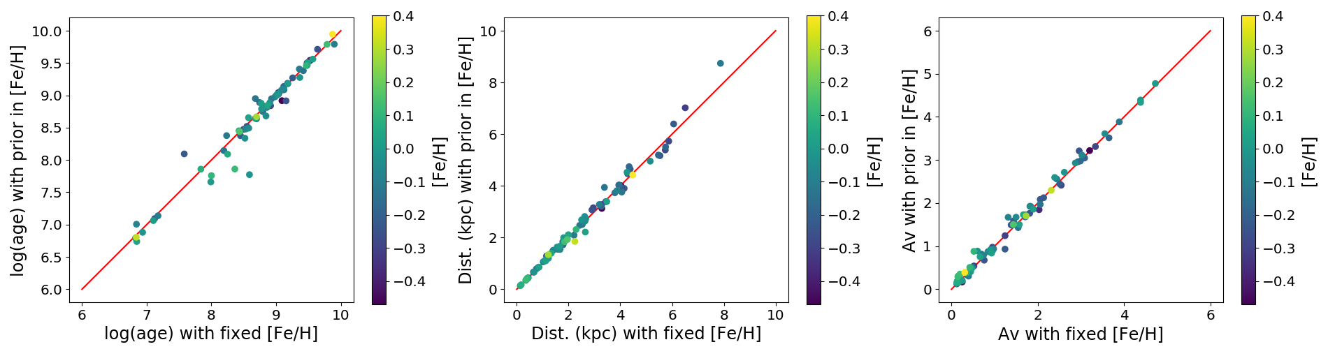
Figure 1: Comparison of results obtained for the fundamental parameters with $[Fe/H]$ held fixed at the value from Carrera et al. (2019) and allowed to vary with a prior based on the Galactic metallicity gradient as described in the text.

Then we look at how the discrepancies in parameter estimates obtained from fits using a prior for $[Fe/H]$ based on the Galactic abundance gradient and fits using $[Fe/H]=0.0$ (which is the usual procedure adopted when this parameter is unknown), when compared to estimates obtained from fits where $[Fe/H]$ is fixed to the values from Carrera et al. (2019) which we take to be the most accurate. In Fig. 2 we show histograms of the discrepancies for log(age), distance and $A_{V}$ in both situations. The histograms show that assuming $[Fe/H]=0.0$ leads to slightly larger discrepancies in log(age) and similar in distance although some outliers are clearly seen. These outliers are all from clusters with CMDs or turn-offs that are not clearly defined. There is a small systematic overestimation of 0.05 mag in $A_{V}$ as well.

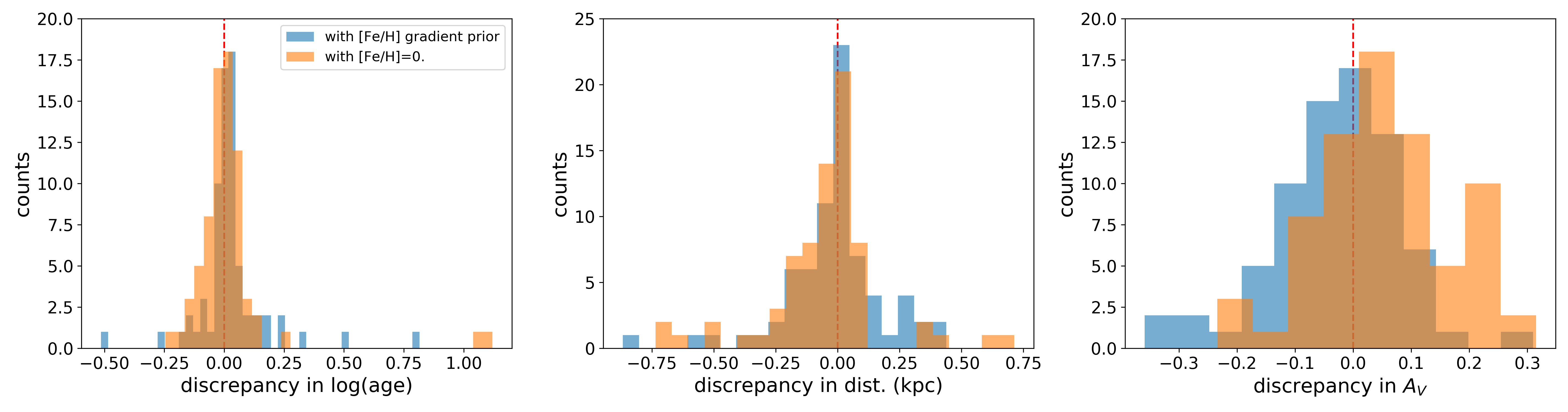
Figure 2: Discrepancies in parameter estimates, obtained from fits using a prior for $[Fe/H]$ based on the Galactic metallicity gradient and fits using $[Fe/H]=0.0$ when compared to estimates obtained from fits where $[Fe/H]$ is fixed to the values from Carrera et al. (2019).

The sensitivity of Gaia data to $[Fe/H]$ can be verified in the results shown in Fig. 3 where the metallicity values obtained from fits using the Galactic abundance gradient prior are compared to values from Carrera et al. (2019) and Netopil et al. (2016). The same behaviour was found for fits where $[Fe/H]$ had no prior albeit with a larger spread, as expected. The average differences from the literature values are $0.014\pm 0.137$ and $0.015\pm 0.127$ with respect to Carrera et al. (2019) and Netopil et al. (2016) respectively. Based on this result we incorporate a baseline error of 0.15 which is combined quadratically with the fit error to give the final uncertainty in $[Fe/H]$.

It is important to point out that this $[Fe/H]$ estimate should not be used as a proper metallicity determination for the open clusters studied. While the derived values of $[Fe/H]$ are indicative of the metallicity of individual clusters, statistically they are based on the metallicity gradient prior and thus cannot be used as a set for determining the Galactic abundance gradient. We have chosen to use $[Fe/H]$ as a free parameter because, as discussed above, it gives less biased results for $A_{V}$ when compared to the widespread practice of adopting $[Fe/H]=0.0$. By letting $[Fe/H]$ vary as a free parameter we also get more reliable estimates and uncertainties in the other parameters. Another positive point in adopting this strategy is that it may indicate clusters where interesting or deviant properties may be present allowing for a sample selection for more detailed observational followup campaigns.

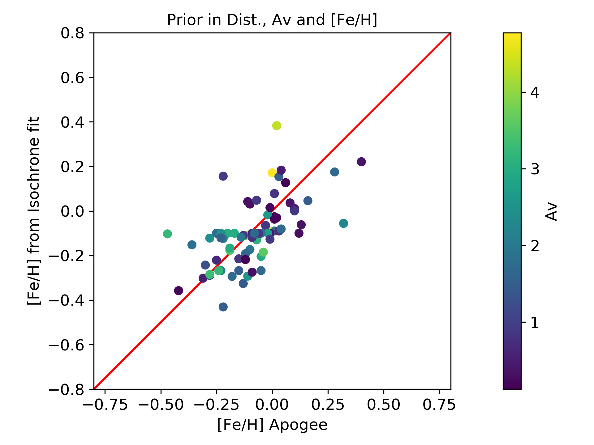
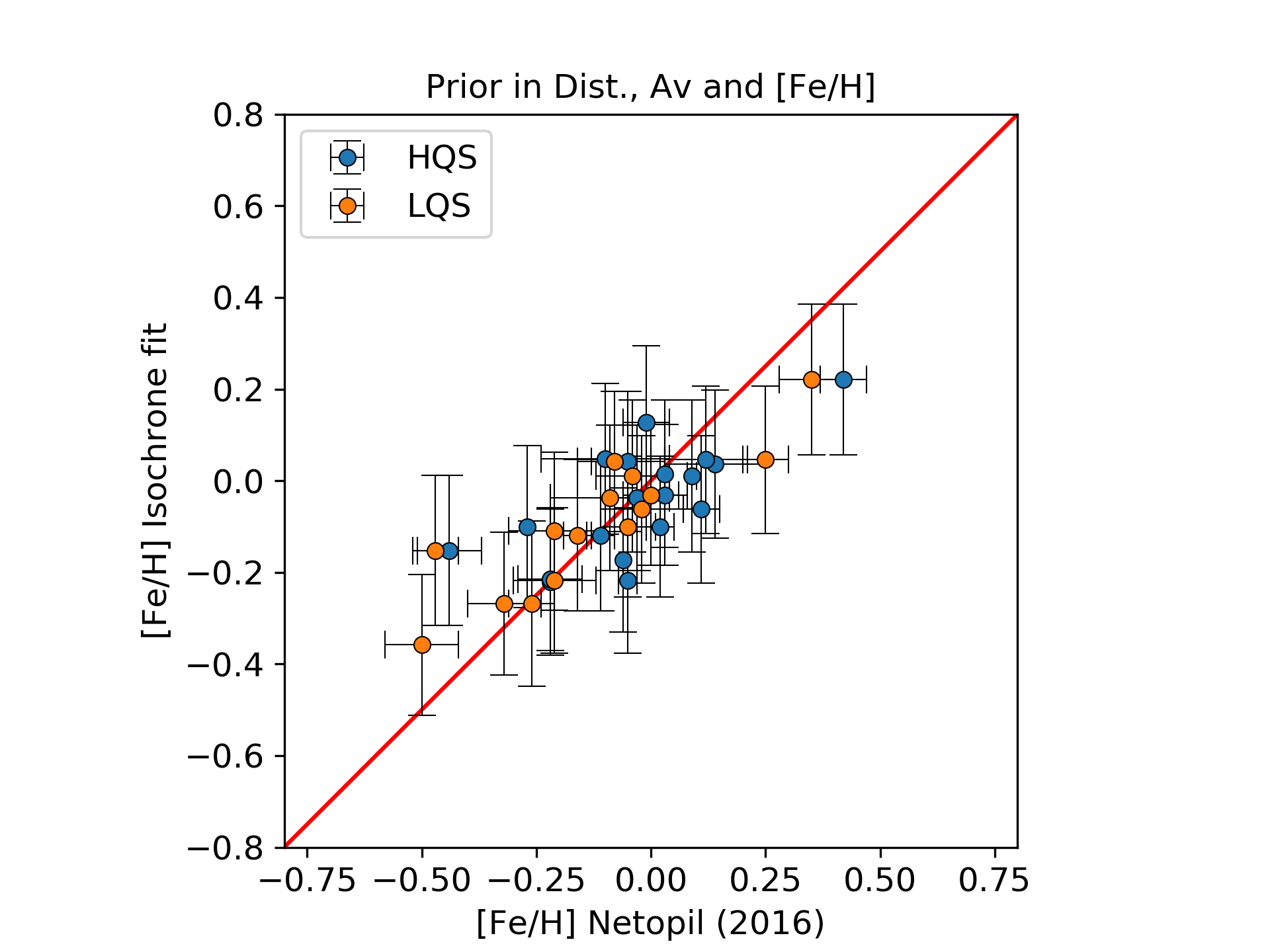
Figure 3: Comparison of $[Fe/H]$ estimates obtained from isochrone fits using the Galactic metallicity gradient as prior to values obtained from the literature. Left panel shows comparison to values from APOGEE from Carrera et al. (2019), where symbols are colored according to $A_{V}$. No systematic deviations due to $A_{V}$ are apparent. Right panel shows comparison to values from Netopil et al. (2016) indicating errors as described in the text and discriminating between the high quality sample (HQS) and the lower quality sample (LQS) as defined by the authors.

As shown above, compared to the fixed $[Fe/H]$ prior from high resolution spectroscopy, adopting the $[Fe/H]$ values determined with the abundance gradient prior does not introduce systematic effects in the other parameters. Based on these results we have adopted the following procedure for the fits in this work: 1) if there is a reliable determination of $[Fe/H]$ in the literature, such as in Carrera et al. (2019) and Netopil et al. (2016) we adopt that value and its uncertainty for the metallicity prior; 2) if there are no reliable value to be used as prior we use a prior based on the Galactic metallicity gradient from Donor et al. (2020). The results of the isochrone fits, using the Galactic metallicity gradient prior, to the clusters with high resolution spectroscopy analyzed in this section are given in Table LABEL:tab:fitsfeh.

5 Results

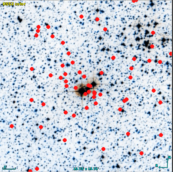
Figure 4: Example of a rediscovered star cluster. Field of $13^{\prime}\times 13^{\prime}$ centered on Hogg 22, with coordinates from Dias et al. (2002). The members of the cluster labelled UBC 547 by Castro-Ginard et al. (2020) are marked in red. In the upper right (N-W) we start seeing a concentration of bright stars which are on the edge of the nearby open cluster NGC 6204.

Of the 75 clusters selected as described in section 2, the membership results for 30 objects either did not reveal identifiable cluster sequences or the isochrone fits were not a good match to the data and were thus discarded from further consideration. These clusters are identified in Table 5. Typically, the fits failed when the sequences were faint and therefore had a small magnitude range, with higher errors, for fitting. While it may seem that our method is not being able to produce results for a high fraction of the clusters, we note that the selected sample of 75 clusters is composed of the leftovers from previous works. Thus, in fact our pipeline has been able to successfully handle 45 remaining considerably difficult cases. The classifications from DAML illustrate the type of objects in our sample: 10 were discovered in infra-red but are visible in the DSS images; Dolidze 1 was classified as possible cluster; Dolidze 35 and ESO 332-13 as a dubious objects; ESO 392-13 was an not found in the DSS images inspection; Sigma Orionis, NGC 1977, and Trapezium were classified as possible OB associations, and ESO 429-02 was classified as a possible open cluster remnant.

With respect to the Trapezium cluster, the situation is further complicated by the presence of other young stellar populations along the same line of sight (Alves & Bouy, 2012; Chen et al., 2019). The cluster here studied is composed of optically revealed, low extinction, elements in the foreground of the embedded Trapezium cluster. It is part of foreground "group 5" in Chen et al. (2019), which includes NGC 1980 and NGC 1981. In this work we identify this stellar aggregate as Trapezium-FG.

During the analysis we found that some clusters reported as new discoveries in recent papers were known clusters listed in DAML. The clusters FoF 2316 and FoF 868 found by Liu & Pang (2019) using using Gaia DR2 have similar positions, parallaxes and proper motions, and coincide with NGC 6530. We note, however, that they are not in the high quality "Class 1" group defined by those authors. Castro-Ginard et al. (2020), also using Gaia DR2, reported the discovery of 582 clusters which they identify under the designation "UBC". Some are known clusters listed in DAML: Czernik 43 $=$ UBC 399; Dolidze 1 $=$ UBC 367; ESO 429 02 $=$ UBC 464; FSR 0761 $=$ UBC 197; Hogg 22 $=$ UBC 547; IC 1442 $=$ UBC 164; NGC 133 $=$ UBC 185; NGC 1977 $=$ UBC 621; NGC 1980 $=$ UBC 208; NGC 6444 $=$ UBC 329; Ruprecht 118 $=$ UBC 313. Fig. 4 illustrates the case of Hogg 22 (UBC 547). Curiously, although Castro-Ginard et al. (2020) mention that NGC1980 is listed in DAML, it is included in the list of newly discovered clusters as UBC 208. We note however that these cases are in small number and do not raise concerns over the much broader scope of findings in Castro-Ginard et al. (2020). They do however highlight how delicate it is to cross-identify open clusters, which are extended objects, not continuous like galaxies, but often sparse discrete groups with irregular shapes, different apparent sizes and without clear boundaries.

For Berkeley 64 we estimated better central coordinates at $\alpha=02^{\rm h}21^{\rm m}45^{\rm s}$; $\delta=+65^{\rm o}53^{\prime}30^{\prime\prime}$ in J2000. For IC 1442 improved central coordinates are $\alpha=22^{\rm h}16^{\rm m}04^{\rm s}$; $\delta=+53^{\rm o}59^{\prime}29^{\prime\prime}$ in J2000, similar to the value estimated by (Maurya et al., 2020).

In the final analysis we also visually checked the color-magnitude diagrams with the isochrone fitted to the $G_{BP}$ and $G_{RP}$ photometric data from Gaia DR2 catalogue. The vector proper motion diagram constructed with individual symbol sizes and colours scaled to the kernel density estimated density in proper motion and parallax space as discussed in Monteiro & Dias (2019), was also checked since in ($\mu_{\alpha}cos{\delta}$, $\mu_{\delta}$, $\varpi$) space a real clusters must show a concentration of stars.

In Table 2 we present the mean astrometric parameters ($\mu_{\alpha}cos{\delta}$, $\mu_{\delta}$, $\varpi$) provided by the method described in section 3.1. In Table 3 the parameters obtained by the isochrone fit are given. In Fig. 7 the final results of the isochrone fit with the stars with membership probability greater than 0.51 are shown.

We point out that the fitting procedure has limitations in the treatment of very young clusters: On the one hand, variable extinction and age spread within the cluster are not specifically included in the fitting model. On the other hand, the grid of PARSEC isochrones does not include ages younger than $\sim$ 4 Myr ($\log$(age) = 6.60) and may not be particularly suited for pre-main sequence (PMS) evolutionary phases. To assess the adequacy of the fits for the youngest objects, we consider the 12 clusters determined to be younger than 10 Myr. For 10 clusters (ESO 332 08, ESO 332 13, FSR 0224, NGC 1980, NGC 6530, NGC 6604, Sigma Orionis, Teutsch 132, Trapezium-FG, vdBergh 130), Fig. 7 shows that while the PMS displays some dispersion, this is not evident on the main sequence which has a large fraction of members. The good definition of the main sequence is indicative that there is no significant variable reddening or age spread ($\lesssim$ 1-2 Myr) for those clusters. The PMS portions of the isochrones display a turn-on to the main sequence that match the observations. Then, at lower masses the isochrones tend to define lower envelopes of the cluster sequence. In terms of the quality of the fits, the PMS and main sequence produce consistent results for these clusters, indicating that the PARSEC isochrones are suitable for analyses of young clusters at least in the Gaia photometric bands (see Lyra et al., 2006, for a discussion on the consistency between PMS and nuclear ages depending on the choice of photometric bands). In any case, with the current pipeline, given the 4 Myr lower age limit of the isochrone grid and the possibility of age spreads, results for clusters found to be younger than $\sim$ 10 Myr should be visually checked and confirmed. The two remaining clusters in the group (Bica 2, FSR 0236) present a clear dispersion on both the main sequence and PMS branches. While it is not clear if the dispersion is due to variable reddening, age spread or a contamination of field stars, it is clear that the results for these two clusters may not be very reliable.

In Fig. 5 we present the comparison of the distances obtained with the isochrone fits with those obtained by using the parallax of the member stars. The distances obtained from parallaxes were determined with a maximum likelihood estimation assuming a normal distribution for individual stars and taking into account individual parallax uncertainties. The standard errors provided in the distance from parallaxes were estimated by considering a symmetric distribution so that $\sigma=r_{95}-r_{5}/(2\times 1.645)$, which is equivalent to 1$\sigma$ Gaussian uncertainty, where $r_{5}$ and $r_{95}$ are 5th and 95th percentile confidence intervals.

The comparison shows a good agreement between the parallax distance and the one obtained via isochrone fitting. After 2.5 kpc a slight tendency for larger distances from parallaxes can be seen, but still within the errors. The result is a clear improvement with respect to the one presented in Monteiro & Dias (2019). While overall the methods are similar in both works, the main difference is that here we use a revised Gaia extinction correction and constrain metallicity with the Galactic abundance gradient prior.

The mean difference in the values is of about 218 pc in the sense of distance from parallaxes minus distance from isochrone fit with a standard deviation of 212 pc. In general, the most discrepant cases are clusters more distant than 5 kpc and whose main sequence is defined below $G=$ 16. In this region the error in parallax increases considerably going from 0.02 mas ($G\leq$14) to typically 0.15 mas at $G=$ 18, leading to relative uncertainties as high as 75%.

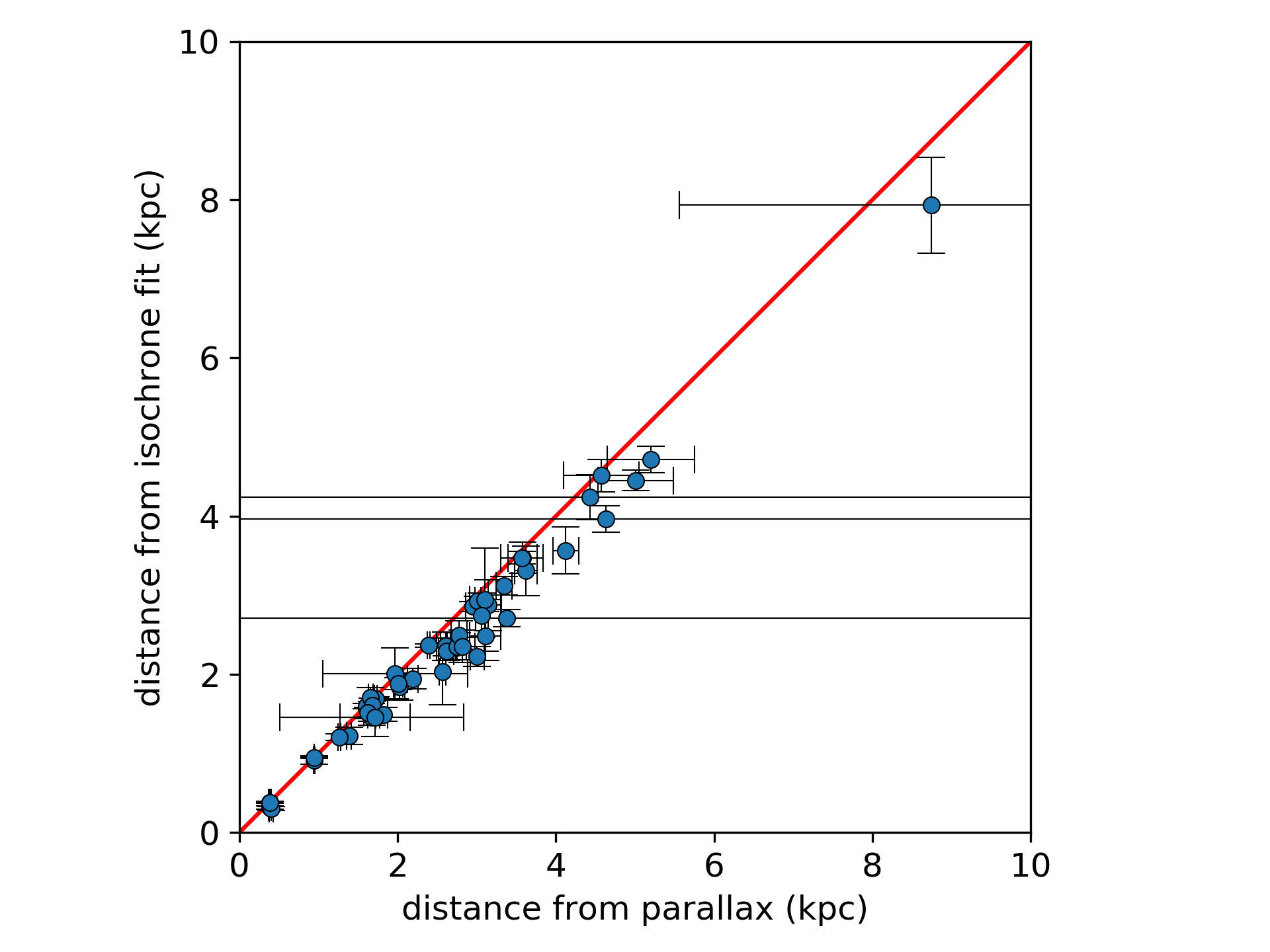
Figure 5: Comparison of distances obtained from parallaxes and isochrone fitting, both based on Gaia DR2.

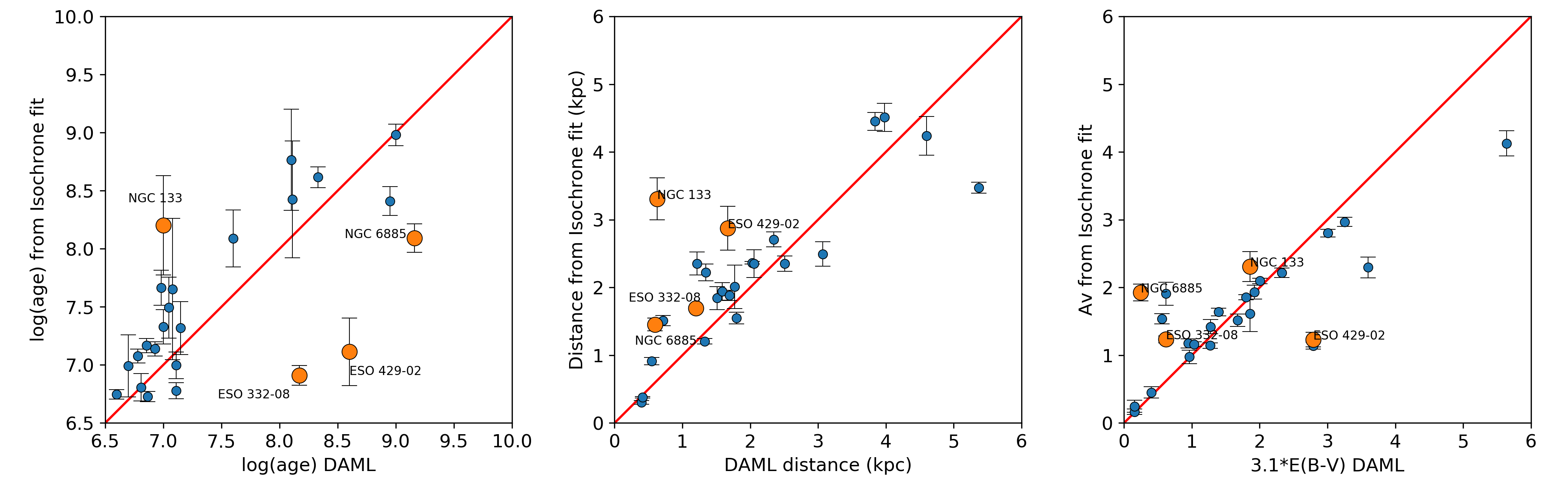
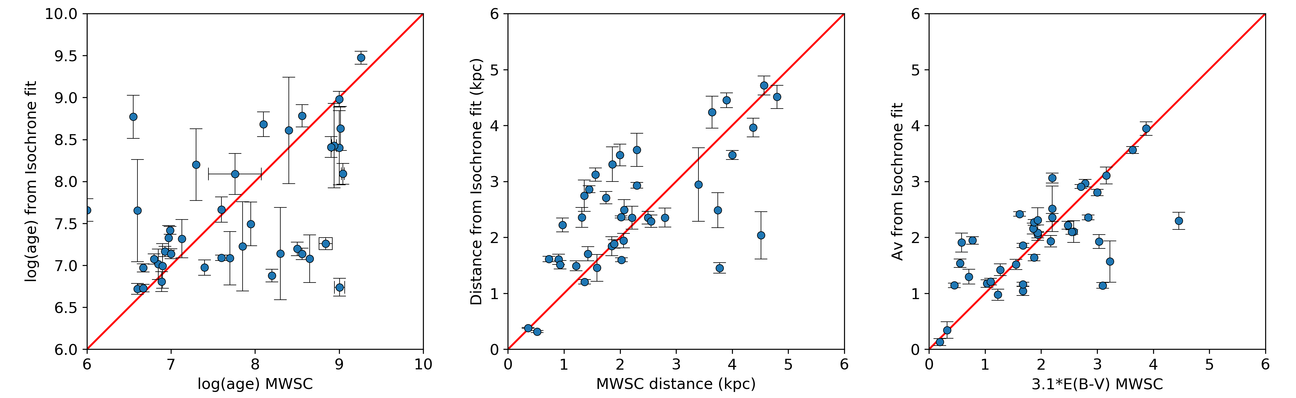
Figure 6: Comparison of the values of distance (left panel), age (middle panel) and $A_{V}$ (right panel) obtained by the isochrone fit with those published in DAML (top) and MWSC (bottom).

Table 2: Results of mean astrometric parameters obtained using the Gaia DR2 stellar proper motion and parallaxes. The meaning of the symbols are as follows: $RA_{ICRS}$ and $DE_{ICRS}$ are the central coordinates of the clusters; $r_{50}$ is the radius in which half of the identified members are located; N is the number of cluster stars; $\mu_{\alpha}cos{\delta}$ and $\mu_{\delta}$ are the proper motion components in mas yr^-1; $\sigma$ is the dispersion of cluster stars’ proper motions; $\varpi$ is the mean parallax of the cluster and $\sigma\varpi$ is the dispersion of the mean parallax. RV and $\sigma RV$ are the mean and 1$\sigma$ dispersion radial velocity obtained for the cluster using Gaia DR2 data and $NRV$ is the number of stars used in the determination of RV after outlier rejection.

Name	$RA_{ICRS}$	$DE_{ICRS}$	$r_{50}$	N	$\mu_{\alpha}cos{\delta}$	$\sigma_{\mu_{\alpha}cos{\delta}}$	$\mu_{\delta}$	$\sigma_{\mu_{\delta}}$	$\varpi$	$\sigma_{\varpi}$	RV	$\sigma_{RV}$	$NRV$
	$(deg)$	$(deg)$	$(deg)$		$(mas)$	$(mas)$	$(mas)$	$(mas)$	$(mas)$	$(mas)$	($kms^{-1}$)	($kms^{-1}$)
BH 88	151.6211	-51.5557	0.056	89	-6.086	0.377	3.602	0.345	0.386	0.165	22.751	1.100	2
Berkeley 64	35.3246	65.8934	0.041	138	-0.551	0.323	0.814	0.408	0.201	0.170
Bica 2	308.3153	41.3068	0.060	140	-2.660	0.244	-4.378	0.230	0.555	0.102
Bochum 10	160.5040	-59.1324	0.148	264	-7.291	0.317	2.992	0.223	0.378	0.092	0.943	0.290	2
Collinder 104	99.1571	4.8155	0.143	179	-1.230	0.411	0.507	0.418	0.514	0.210
Czernik 43	351.4483	61.3294	0.057	173	-3.862	0.317	-2.078	0.244	0.350	0.134
DC 3	111.7507	-37.5195	0.025	105	-1.214	0.331	2.645	0.472	0.081	0.189
Dolidze 1	302.4057	36.5052	0.075	226	-2.721	0.312	-4.961	0.326	0.288	0.118
Dolidze 35	291.3465	11.6414	0.064	91	-1.967	0.245	-4.322	0.392	0.288	0.181	22.577	0.174	2
ESO 123 26	118.1254	-60.3348	0.105	22	-3.572	0.318	10.909	0.180	1.026	0.044
ESO 332 08	253.6906	-40.7299	0.080	201	-0.272	0.316	-1.348	0.313	0.529	0.200
ESO 332 13	254.1701	-40.5887	0.058	52	-0.080	0.225	-1.117	0.237	0.558	0.127
ESO 392 13	261.7178	-34.7020	0.092	21	1.690	0.262	-2.882	0.176	0.900	0.139
ESO 429 02	113.3481	-28.1816	0.050	54	-2.806	0.199	3.673	0.292	0.281	0.155
FSR 0224	306.3509	40.2243	0.021	19	-3.242	0.343	-4.373	0.268	0.566	0.068
FSR 0236	308.1682	41.4418	0.048	89	-2.491	0.394	-4.076	0.243	0.522	0.163
FSR 0377	338.7186	58.3041	0.044	116	-3.219	0.366	-2.155	0.301	0.207	0.159
FSR 0441	355.5402	58.5480	0.040	95	-2.049	0.313	-1.160	0.220	0.239	0.169
FSR 0591	36.9315	58.7637	0.057	222	-0.231	0.571	-0.566	0.484	0.293	0.214	-72.562	0.864	2
FSR 0674	63.0983	48.7296	0.033	49	-0.894	0.419	-0.871	0.243	0.275	0.285
FSR 0761	83.3381	39.8388	0.034	85	0.323	0.350	-1.361	0.334	0.253	0.145	-27.299	1.923	2
FSR 1443	129.8570	-47.3566	0.054	154	-3.563	0.382	4.147	0.439	0.220	0.171	37.746	1.384	2
FSR 1698	230.2346	-59.6270	0.044	161	-4.033	0.341	-3.524	0.307	0.247	0.224
Hogg 16	202.2997	-61.2087	0.047	46	-3.479	0.095	-1.645	0.146	0.431	0.065
Hogg 22	251.6599	-47.0782	0.044	117	-0.750	0.254	-2.013	0.339	0.343	0.138
IC 1442	334.0070	53.9900	0.058	333	-3.083	0.484	-2.884	0.476	0.240	0.198
Majaess 65	87.4284	27.0746	0.120	51	-0.258	0.229	-1.063	0.320	0.974	0.160
NGC 133	7.8324	63.3583	0.068	284	-2.324	0.431	-0.410	0.250	0.223	0.158	-86.916	0.405	5
NGC 1977	83.7945	-4.8018	0.145	93	1.260	0.453	-0.569	0.520	2.590	0.185	27.392	2.361	6
NGC 1980	83.8212	-5.9207	0.125	120	1.192	0.388	0.511	0.385	2.583	0.128	25.264	7.055	8
NGC 2384	111.2913	-21.0211	0.063	80	-2.303	0.185	3.118	0.220	0.330	0.132
NGC 6200	251.0322	-47.4582	0.109	433	-0.950	0.333	-2.244	0.351	0.307	0.265
NGC 6444	267.3950	-34.8221	0.059	47	-0.934	0.114	-0.929	0.096	0.521	0.073
NGC 6530	271.1088	-24.3572	0.087	80	1.375	0.352	-1.992	0.307	0.762	0.111
NGC 6604	274.5127	-12.2449	0.049	88	-0.453	0.208	-2.294	0.314	0.454	0.134
NGC 6885	302.9831	26.4935	0.137	726	-3.127	0.356	-5.471	0.413	0.439	0.245	2.378	0.333	4
Ruprecht 118	246.1454	-51.9544	0.051	79	-3.152	0.188	-4.345	0.174	0.285	0.107
Ruprecht 123	260.7813	-37.8977	0.055	20	1.044	0.172	0.922	0.108	0.604	0.084
Ruprecht 55	123.1133	-32.5815	0.064	414	-2.316	0.394	2.921	0.436	0.187	0.174	64.253	1.769	2
SAI 43	77.0723	49.8645	0.035	135	0.611	0.390	-0.555	0.389	0.109	0.280
Sigma Orionis	84.6860	-2.5959	0.054	45	1.336	0.388	-0.633	0.372	2.479	0.157
Stock 3	18.0592	62.3190	0.060	114	-1.895	0.326	-0.357	0.296	0.265	0.132
Teutsch 132	77.5140	38.8163	0.057	112	0.326	0.506	-1.536	0.329	0.223	0.234
Trapezium-FG	83.8350	-5.4095	0.352	269	1.262	0.449	0.274	0.498	2.557	0.149	23.841	5.161	15
vdBergh 130	304.4624	39.3404	0.049	62	-3.609	0.308	-5.075	0.292	0.521	0.154

Table 3: Fundamental parameters obtained from the isochrone fits. The last two columns give the distances estimated from parallaxes with a maximum likelihood estimation assuming a normal distribution and taking into account individual parallax uncertainties. The standard errors provided in the distance from parallaxes were estimated considering the calculated 5th and 95th percentile confidence intervals assuming a symmetric distribution so that $\sigma=r_{95}-r_{5}/(2\times 1.645)$, which is equivalent to 1$\sigma$ Gaussian uncertainty. The 0.029 mas correction (Lindegren et al., 2018) to the mean parallaxes was previously added.

Name	$dist$	$\sigma_{dist}$	$age$	$\sigma_{age}$	$[Fe/H]$	$\sigma_{[Fe/H]}$	$A_{V}$	$\sigma_{A_{V}}$	$dist_{\pi}$	$\sigma_{dist_{\pi}}$
	$(pc)$	$(pc)$	$(dex)$	$(dex)$	$(dex)$	$(dex)$	$(mag)$	$(mag)$	$(pc)$	$(pc)$
BH 88	2011	321	8.766	0.435	-0.141	0.228	1.612	0.262	1936	1115
Berkeley 64	4547	378	8.926	0.046	-0.203	0.171	2.951	0.043	4889	812
Bica 2	1550	85	6.746	0.041	0.100	0.214	4.126	0.186	1665	40
Bochum 10	2365	19	7.167	0.061	0.179	0.172	1.175	0.066	2390	18
Collinder 104	1599	35	7.197	0.081	-0.104	0.171	2.104	0.195	1609	25
Czernik 43	2350	113	8.088	0.245	-0.023	0.160	1.931	0.103	2616	74
DC 3	7934	607	9.474	0.076	-0.146	0.158	1.042	0.082	8744	3184
Dolidze 1	2860	63	7.090	0.032	0.054	0.177	2.049	0.056	2949	95
Dolidze 35	2334	98	7.952	0.466	0.204	0.180	3.987	0.050	2603	122
ESO 123 26	914	55	8.616	0.089	0.065	0.191	0.451	0.084	948	9
ESO 332 08	1693	22	6.911	0.085	0.230	0.187	1.234	0.053	1723	15
ESO 332 13	1487	84	6.840	0.139	0.168	0.183	1.380	0.027	1673	51
ESO 392 13	1032	85	8.656	0.428	0.074	0.185	1.906	0.201	1057	22
ESO 429 02	2875	322	7.113	0.291	-0.120	0.195	1.233	0.108	3141	170
FSR 0224	1706	127	6.739	0.106	0.242	0.266	3.061	0.091	1659	29
FSR 0236	1610	91	6.877	0.076	0.091	0.198	3.564	0.062	1678	28
FSR 0377	3563	297	7.085	0.317	-0.065	0.175	2.159	0.098	4124	162
FSR 0441	3473	196	7.079	0.285	-0.153	0.177	2.419	0.039	3579	183
FSR 0591	2930	52	7.014	0.182	-0.187	0.205	2.270	0.052	3014	39
FSR 0674	2944	656	8.782	0.134	-0.140	0.156	3.107	0.150	3106	193
FSR 0761	2485	312	8.770	0.258	-0.112	0.205	1.568	0.368	3107	193
FSR 1443	3303	157	8.703	0.416	-0.019	0.159	1.819	0.159	3444	60
FSR 1698	3122	118	7.136	0.068	0.228	0.163	2.907	0.035	3341	95
Hogg 16	1943	131	7.494	0.262	0.110	0.206	1.422	0.107	2190	68
Hogg 22	2354	171	7.076	0.060	0.120	0.170	2.097	0.040	2749	123
IC 1442	2710	112	7.665	0.151	-0.100	0.160	1.271	0.277	3378	9075
Majaess 65	944	10	8.207	0.167	0.006	0.160	0.768	0.105	945	4
NGC 133	3308	311	8.201	0.427	-0.133	0.163	2.310	0.222	3615	142
NGC 1977	381	9	6.721	0.064	-0.184	0.170	0.344	0.148	388	27
NGC 1980	316	19	6.970	0.049	-0.242	0.175	0.129	0.060	384	18
NGC 2384	2494	179	7.318	0.228	-0.147	0.257	0.976	0.098	2775	99
NGC 6200	2352	205	7.138	0.060	0.166	0.193	1.858	0.038	2821	152
NGC 6444	1492	88	8.632	0.262	0.177	0.191	1.298	0.130	1823	54
NGC 6530	1206	39	6.728	0.045	0.373	0.203	1.163	0.037	1265	18
NGC 6604	1885	75	6.807	0.118	0.104	0.222	2.804	0.057	2007	59
NGC 6885	1453	95	8.092	0.124	0.055	0.192	1.927	0.123	1671	1466
Ruprecht 118	2224	125	8.425	0.503	0.386	0.196	1.144	0.041	3004	88
Ruprecht 123	1511	74	8.682	0.147	0.188	0.224	1.909	0.169	1622	48
Ruprecht 55	4238	286	7.328	0.148	-0.226	0.154	1.639	0.056	4430	43070
SAI 43	4451	131	8.410	0.124	-0.198	0.172	1.538	0.075	5009	480
Sigma Orionis	303	26	6.997	0.114	-0.092	0.158	0.166	0.040	402	25
Stock 3	2747	281	7.226	0.531	-0.100	0.168	2.355	0.073	3051	84
Teutsch 132	3474	81	6.992	0.266	-0.160	0.206	2.217	0.069	3567	267
Trapezium-FG	381	12	6.778	0.069	-0.146	0.160	0.246	0.089	386	1
vdBergh 130	1456	240	6.974	0.091	-0.029	0.222	2.356	0.042	1714	563

6 Comparison with the literature

The comparison presented here has two goals: to provide an extra sanity check of our results and to assess the improvement they bring. To this end we base the analysis on the widely used DAML and Kharchenko et al. (2013) (hereafter MWSC) catalogues. It is important to note that these are different types of catalogues. On the one hand, the MWSC is the output of a program applied to the PPMXL (Roeser et al., 2010) and 2MASS (Skrutskie et al., 2006) data. On the other hand, DAML is a compilation, curated by humans, of the best results (judged by the curators) available in the literature. The MWSC aims to overcome the non-uniformity in compilations from the literature, which are based on results obtained by different authors using different techniques, models and calibrations. However, as pointed out in Moitinho (2010) homogeneous methods do not necessarily produce the best results. As an example, for close objects, parallaxes provide the best distances, but at larger distances isochrone fits are better. Assuming the algorithm employed in the MWSC is flawless, the relatively shallow data used in the MWSC limits its usefulness to bright and/or close clusters.

The DAML catalogue is a compilation of results from the literature. While it is non-homogeneous in nature, it is curated. The curators choose the best results, when more than one is available, and keep public logs of what has changed, of the references to the catalogued parameters and a list of objects that studies have shown not to be real clusters as well as the references to those studies. As a compilation, it also includes results from the MWSC. Thus, the comparison with DAML is also a comparison with individual studies from the literature.

The cross-identification of our sample with DAML and with the MWSC results in 45 and 40 objects in common, respectively. Since DAML also contains values from the MWSC, the later were not included in the DAML plots to avoid comparing the same points twice. This leaves the DAML comparison sample with 28 clusters. The comparisons of distance, age and $A_{V}$ are shown in Fig. 6.

The $A_{V}$ and distances from both catalogs follow the same trend as those obtained with our isochrone fits, although with some considerable scatter (clearly higher in the case of the distances from MWSC) and with a tendency for smaller catalogued distances for the closer ($<$ 3 kpc) sub-sample. The same trend in the distances can be observed when comparing the distances estimated from the parallaxes of clusters published in Cantat-Gaudin & Anders (2020) with respect to the DAML and MWSC catalogues.

The age comparison shows a much high dispersion. In the case of the MWSC, ages appear to be almost uncorrelated to the ones here determined, except for a small group of clusters younger than $\sim$ 10 Myr (in the MWSC age scale). In the DAML age comparison we find 4 especially discrepant objects. They are ESO 332-08, ESO 429-02, NGC 133 and NGC 6885.

The cluster sequences for ESO 332-08 and NGC 6885 presented in Fig. 7 are well defined and the isochrone fits are clearly adequate. The parameters in DAML for NGC 6885 are from Lyngå (1988). For ESO 332-08 the parameters were taken from Kharchenko et al. (2005). We note that the same authors later published the MWSC with revised parameters for ESO 332-08, although the ages coincide in both catalogues. DAML kept the previous version, which listed a larger distance presenting a better fit to CMDs. The isochrone fit in Fig. 7 confirms that the distance in Kharchenko et al. (2005) is more accurate than the one in the MWSC.

NGC 133 is the most discrepant cluster in the sample. It is visually identified in DSS images from a small group of bright stars. The CMD in Fig. 7 displays a bifurcation around $G\sim$ 16 mag, leading to a redder evolved branch that our isochrone fit follows, but does not include the bright stars. The blue branch does include the brighter stars, which is what Carraro (2002) identifies as NGC 133 and results in the parameters listed in DAML. A possibility would be that we are looking at different objects along the same line of sight. However, both branches display the same proper motions and have probable members, which together with the sparseness of the blue branch indicates that the apparently younger sequence is composed of blue stragglers in NGC 133. We conclude that the cluster now revealed by Gaia DR2 is in fact older than previously estimated.

ESO 429-02 is an interesting case. The cluster sequence revealed by its members is sparse, but still clearly young with a pronounced pre-main-sequence (PMS) well fitted by the $logt=$ 7.1 isochrone in Fig. 7 once taking into account the relatively high (variable) extinction and variability in the PMS phase. The parameters in DAML come from the analysis of 2MASS photometry and UCAC2 astrometry done by Pavani & Bica (2007). Despite the above mentioned limitations of these data-sets, their work reveals a CMD that although poor, can be plausibly reproduced by an older $logt=$ 8.6 isochrone. An inspection of the Gaia DR2 proper motion vector point diagram reveals two over-densities, in which the stronger peak corresponds to the sequence identified in our work. It is a possible case of two different objects along the same line of sight.

Of the 11 mean radial velocities of open clusters determined here, 6 are in common with DAML (Bochum 10, NGC 6885, Trapezium-FG, NGC 1980, NGC 1977 and Ruprecht 55) published by Dias et al. (2014). The comparison of this small sample shows discrepancies ranging from -29 $kms^{-1}$ to 4 $kms^{-1}$. Considering that the memberships presented in this work are superior to those published in Dias et al. (2014), we believe the radial velocity estimates in this work are more reliable.

In the previous sections we validated our cluster parameter determination procedure by comparing distances with those from from Gaia DR2 parallaxes and metallicities with those from high resolution spectroscopy. In this section we confirm that in general, while following the same trend as those from pre-Gaia studies, our determinations, represent a substantial improvement over the previous values. It is also interesting how the comparisons clearly show that in this case, a non-homogeneous compilation of parameters (DAML) can provide a more accurate data-set than an homogeneously derived catalogue (MWSC). We note, however, that this is seen because we removed the the MWSC values from the DAML sample.

7 Conclusions

We have investigated 45 open clusters with Gaia DR2. From the astrometric data (proper motions and parallaxes) we determined their stellar membership probabilities, taking into account the full co-variance matrix of the data.

For all clusters we estimated mean proper motion and mean parallax considering the member stars (membership $\geq$ 0.51). Mean radial velocities were determined for 12 clusters, 7 of them for the first time, although based on small numbers of members with available Gaia DR2 radial velocity measurements. The fundamental parameters age, distance and $A_{V}$ were estimated with a new version of the global optimization code presented in Monteiro et al. (2017) applied to $G_{BP}$ and $G_{RP}$ photometry using a revised extinction polynomial law for Gaia DR2 and the Galactic abundance gradient as a prior for metallicity. The new procedure was validated using a sample of clusters in the literature for which high resolution spectroscopy was available. Our isochrone fitting results for a high resolution spectroscopy sample are also presented. We verify that the PMS portions of the PARSEC isochrones fit well the cluster sequences, consistently with the main sequence fit, indicating that they are suitable for analyses of young clusters (down to 4 Myr) at least in the Gaia photometric bands.

This study provides the first determination of distance and age for the cluster Majaess 65 and of age for Ruprecht 123. The cluster DC 3 is found to be one of the oldest (5.6 Gyr) and most distant ($\sim$7900 pc) known open clusters.

We assessed the quality of our results by comparing with distances from parallaxes, metallicities from high resolution spectroscopy and a critic inspection of the literature. In the process, we identified several clusters reported as new discoveries in recent papers based on Gaia DR2 that were already known clusters listed in DAML. We find that our cluster parameter determinations, represent a substantial improvement over the previous values.

This work is part of an ongoing project that will bring DAML to the Gaia era.

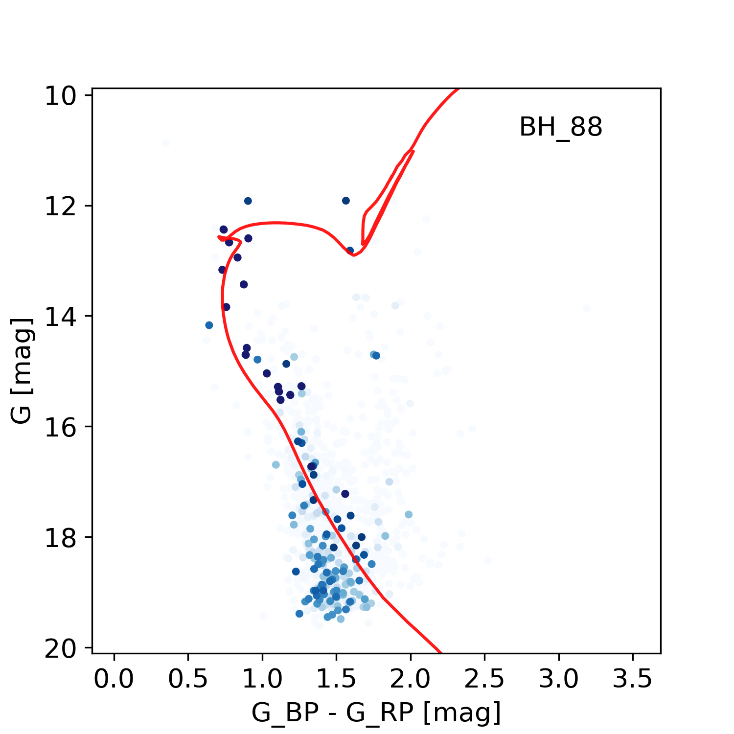
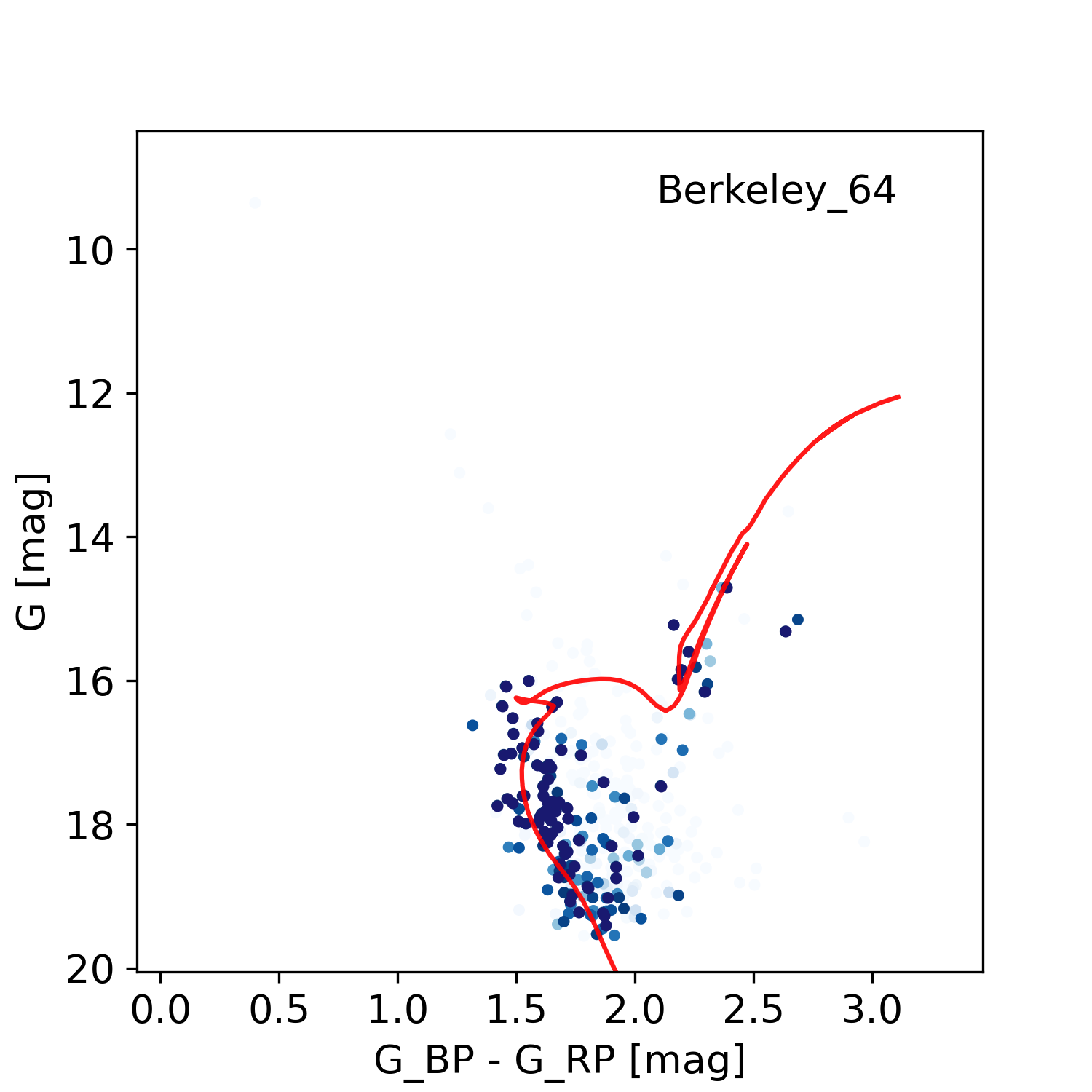
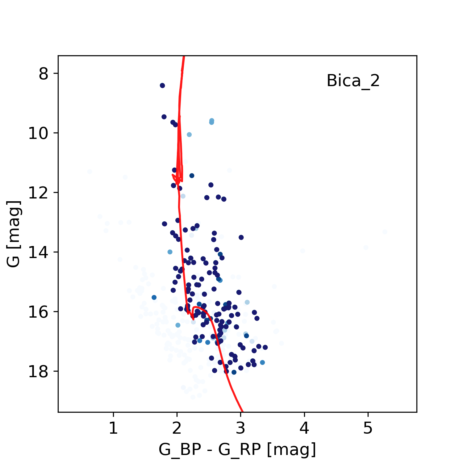
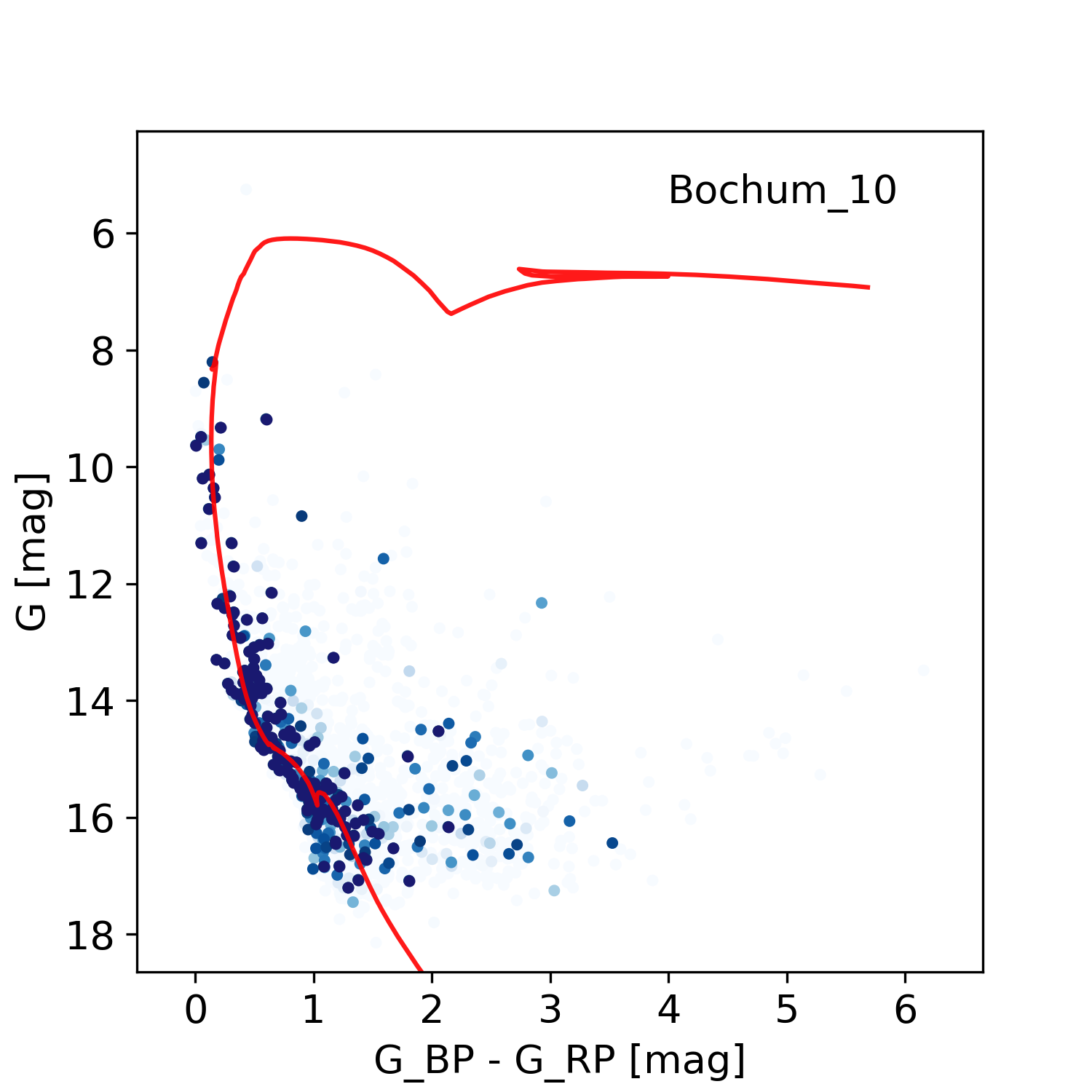
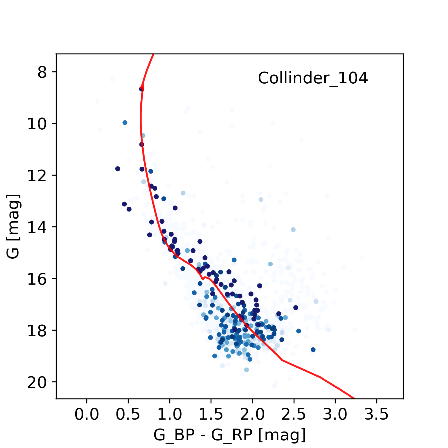
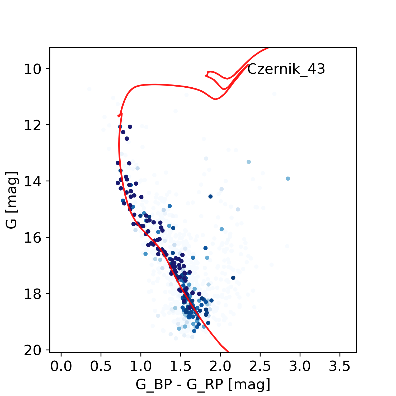
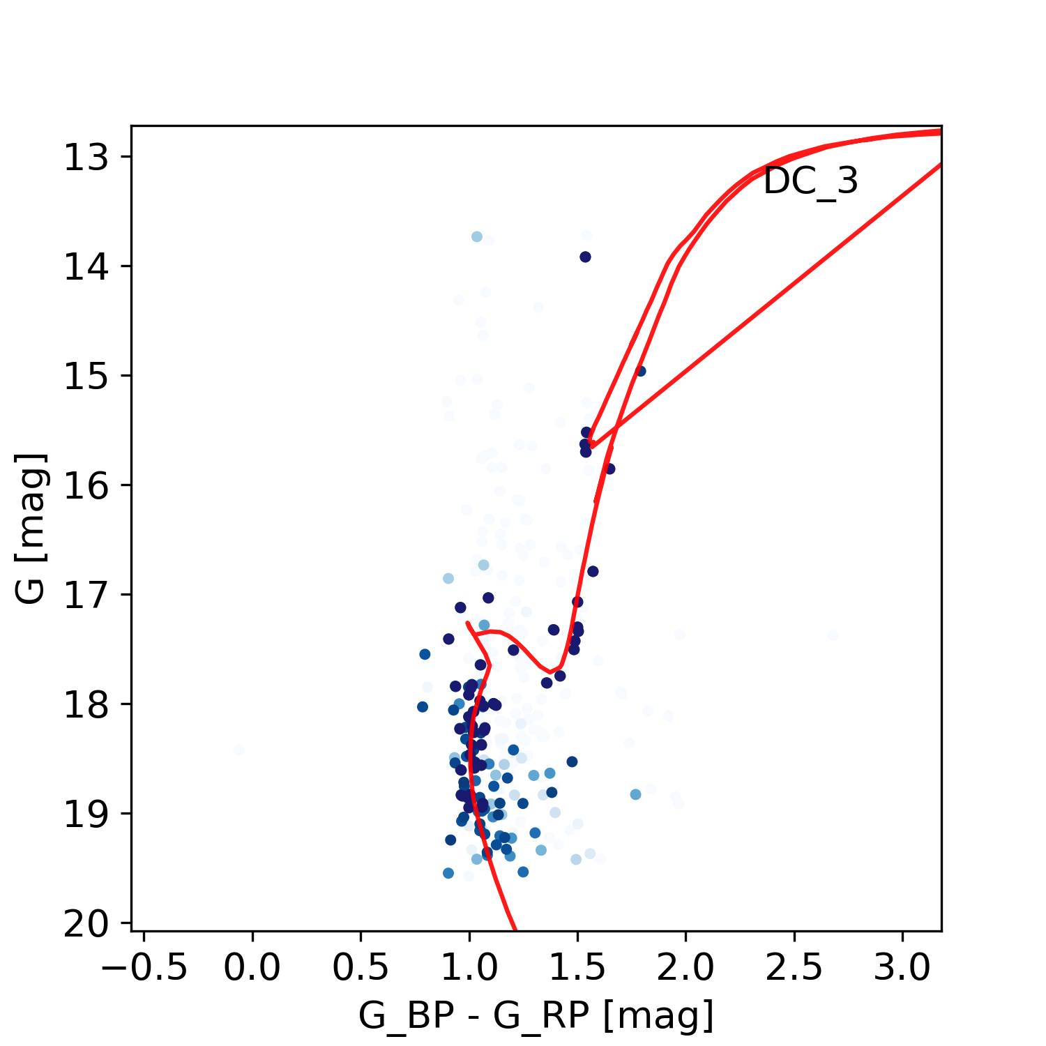
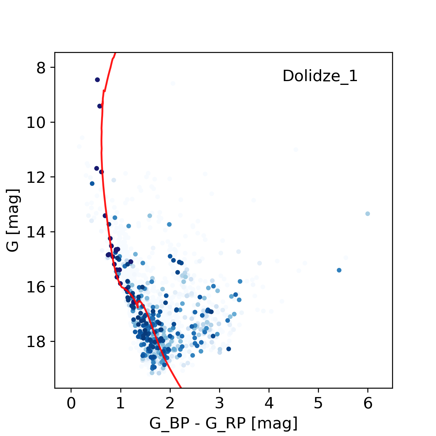
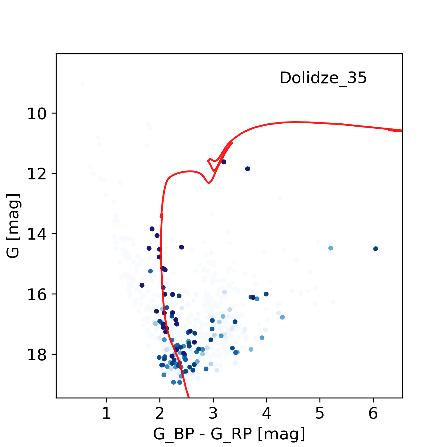
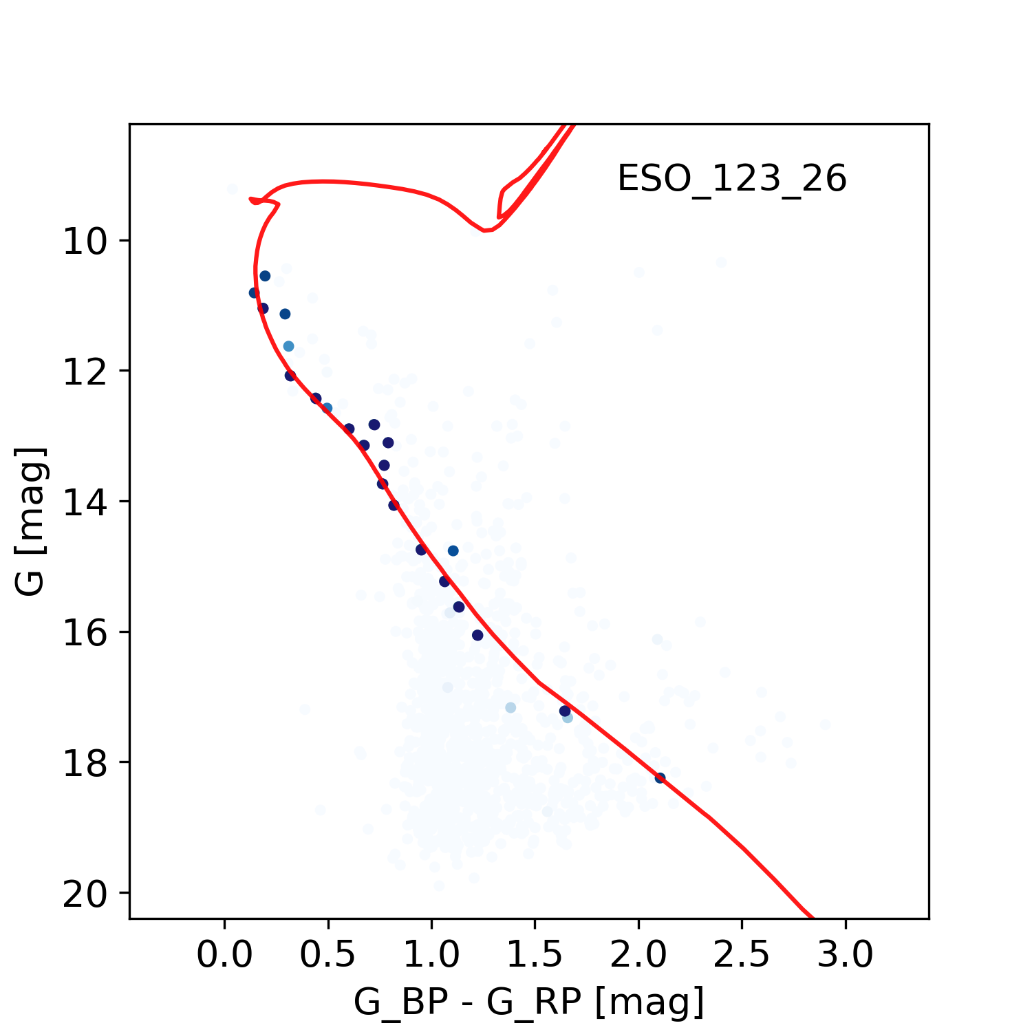
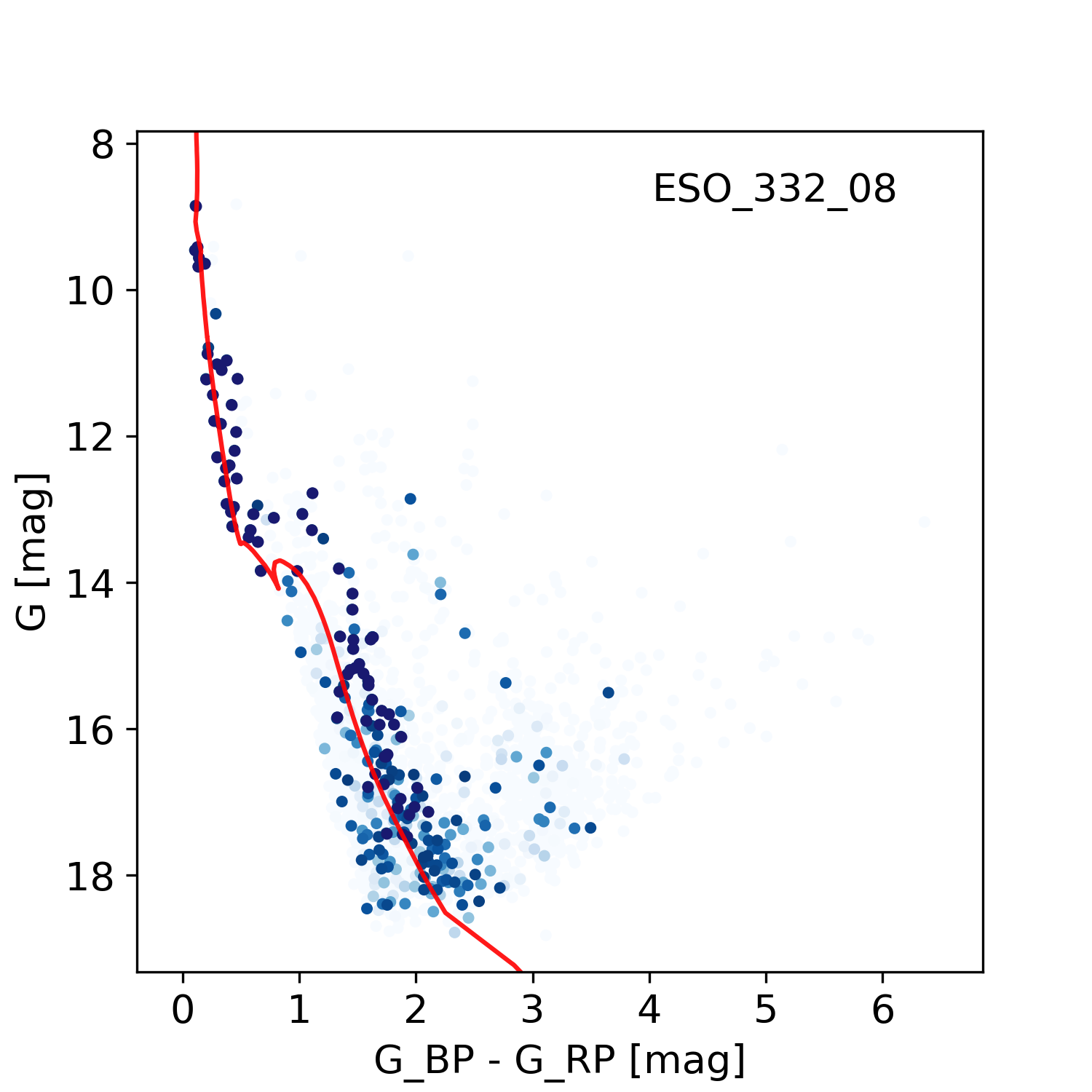
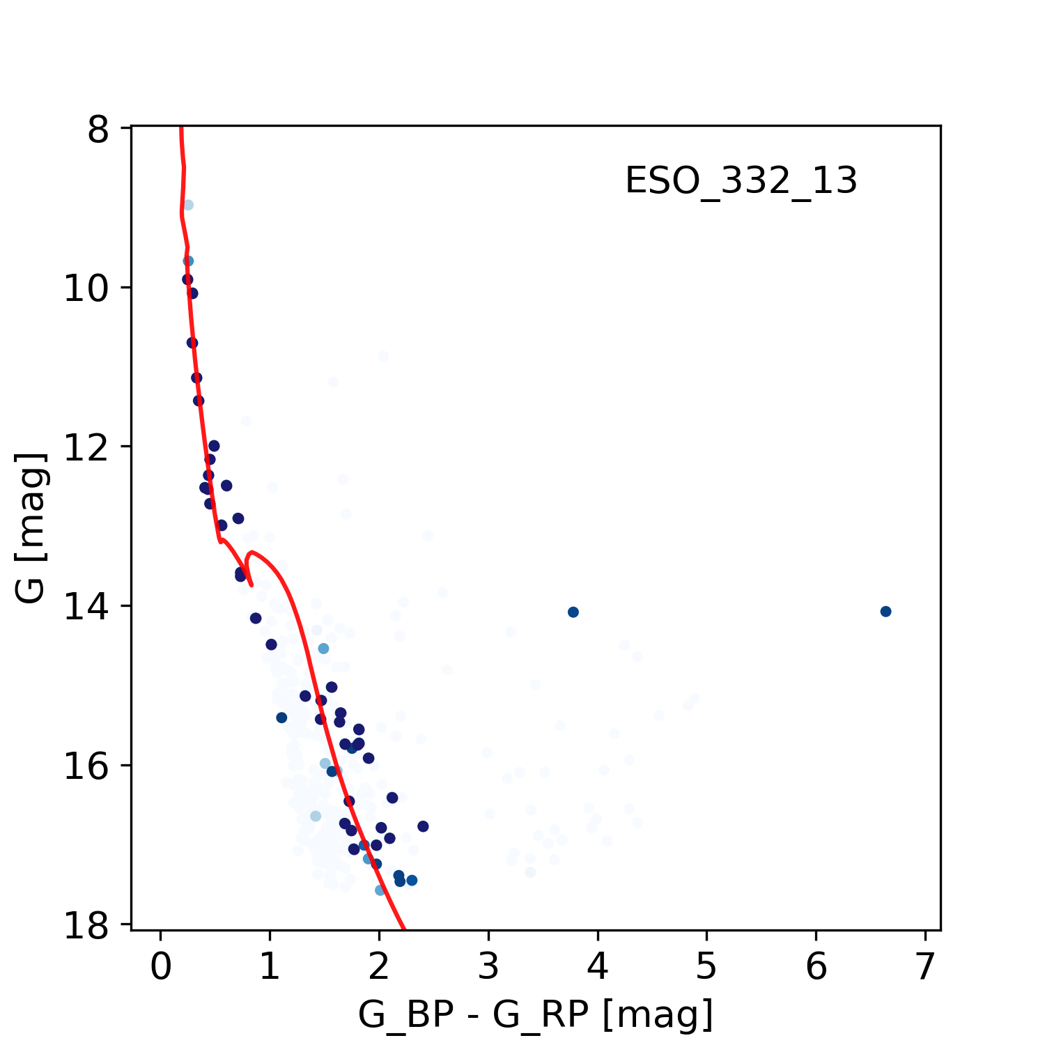
Figure 7: CMDs and isochrone fits to the Gaia DR2 data for the clusters investigated in this study. Probable member stars are shown in blue dots, with more intense tones indicating higher membership probability. The light-gray dots mark non-member stars in the field.

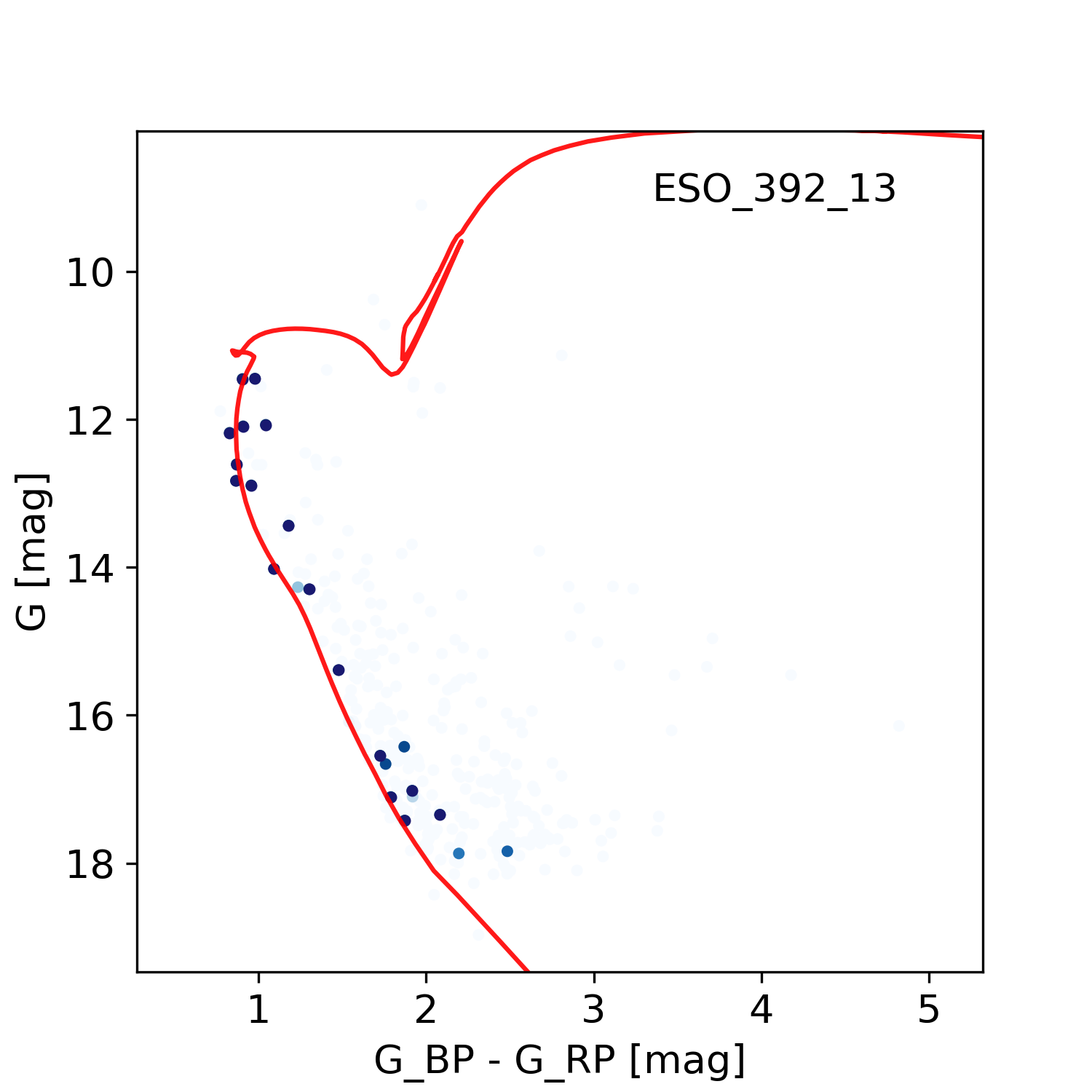
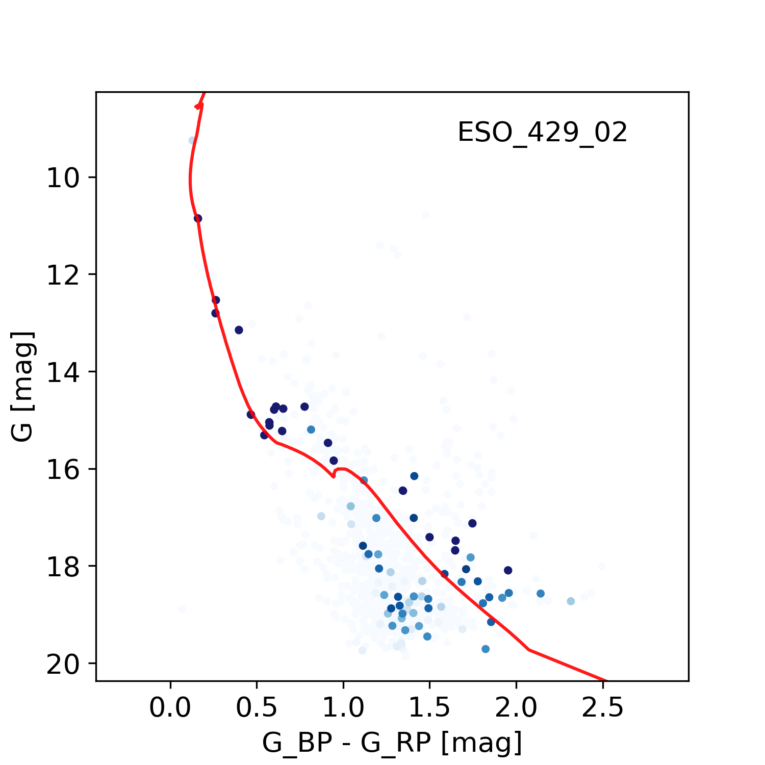
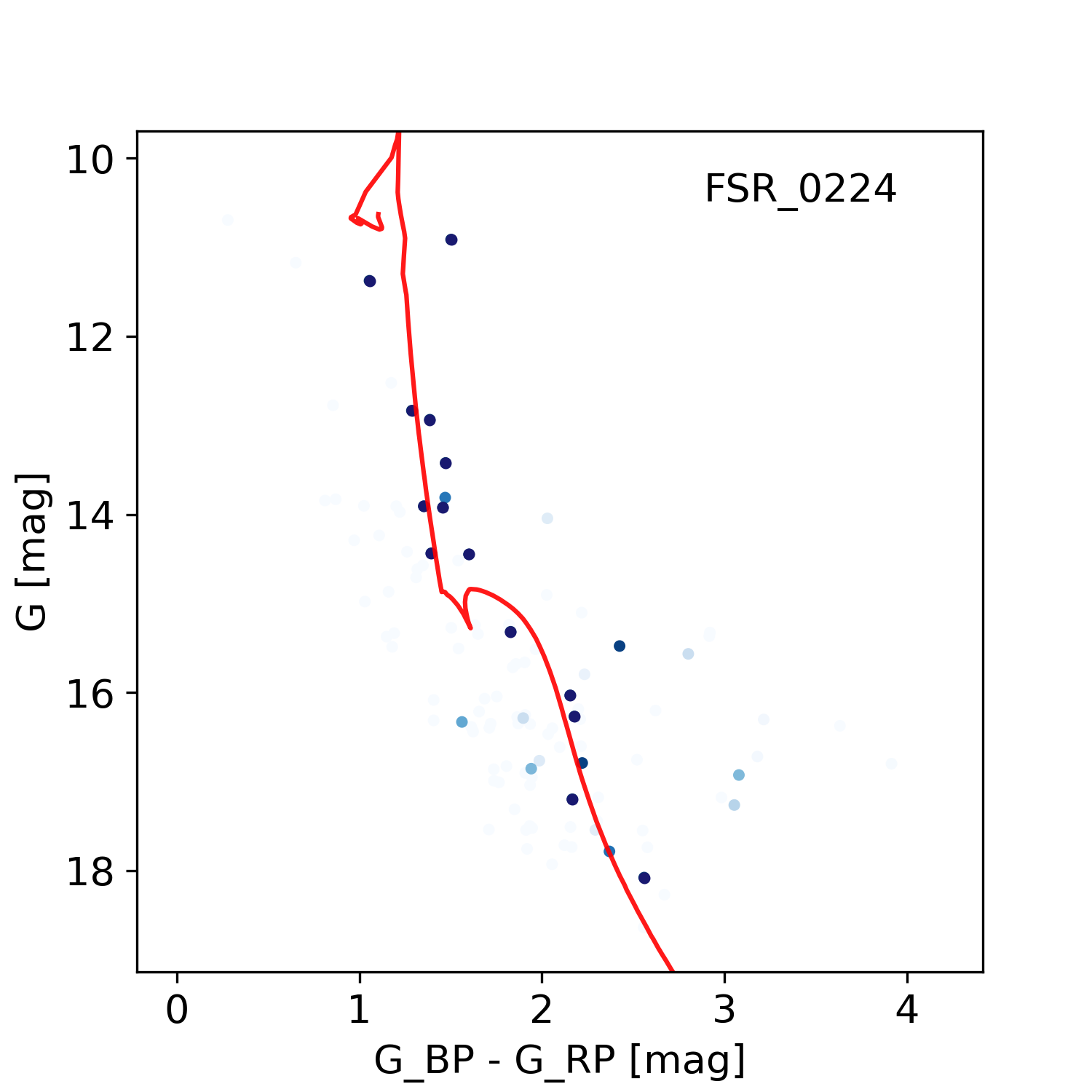
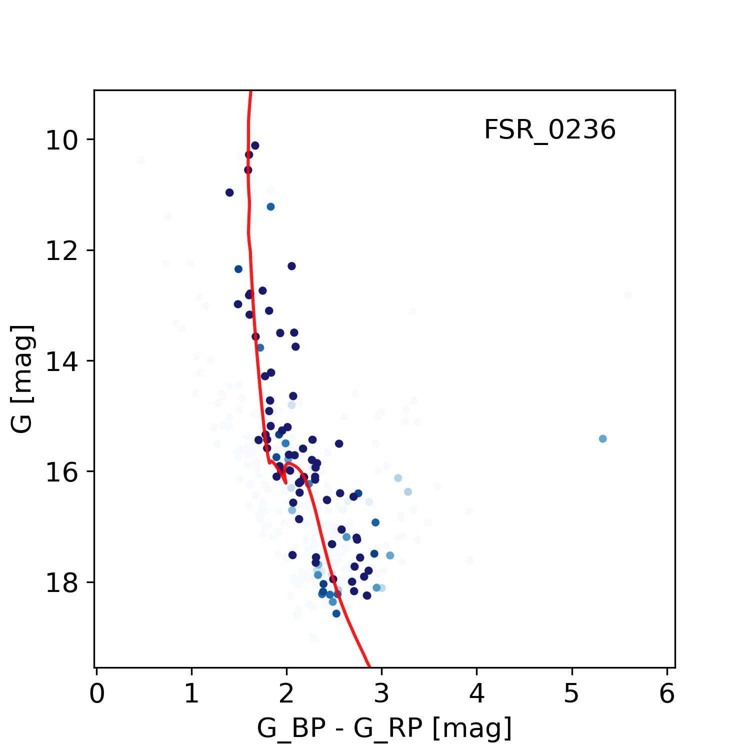
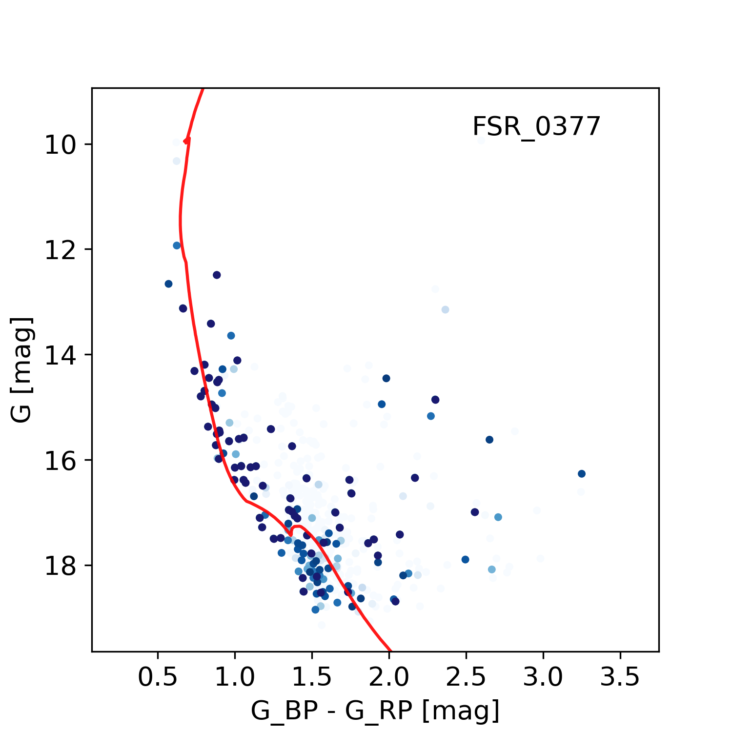
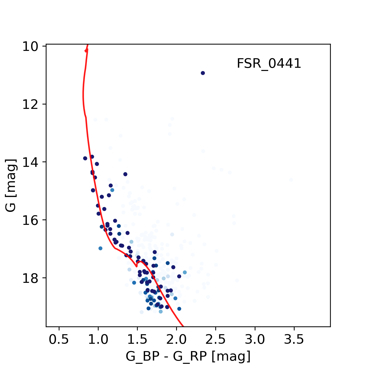
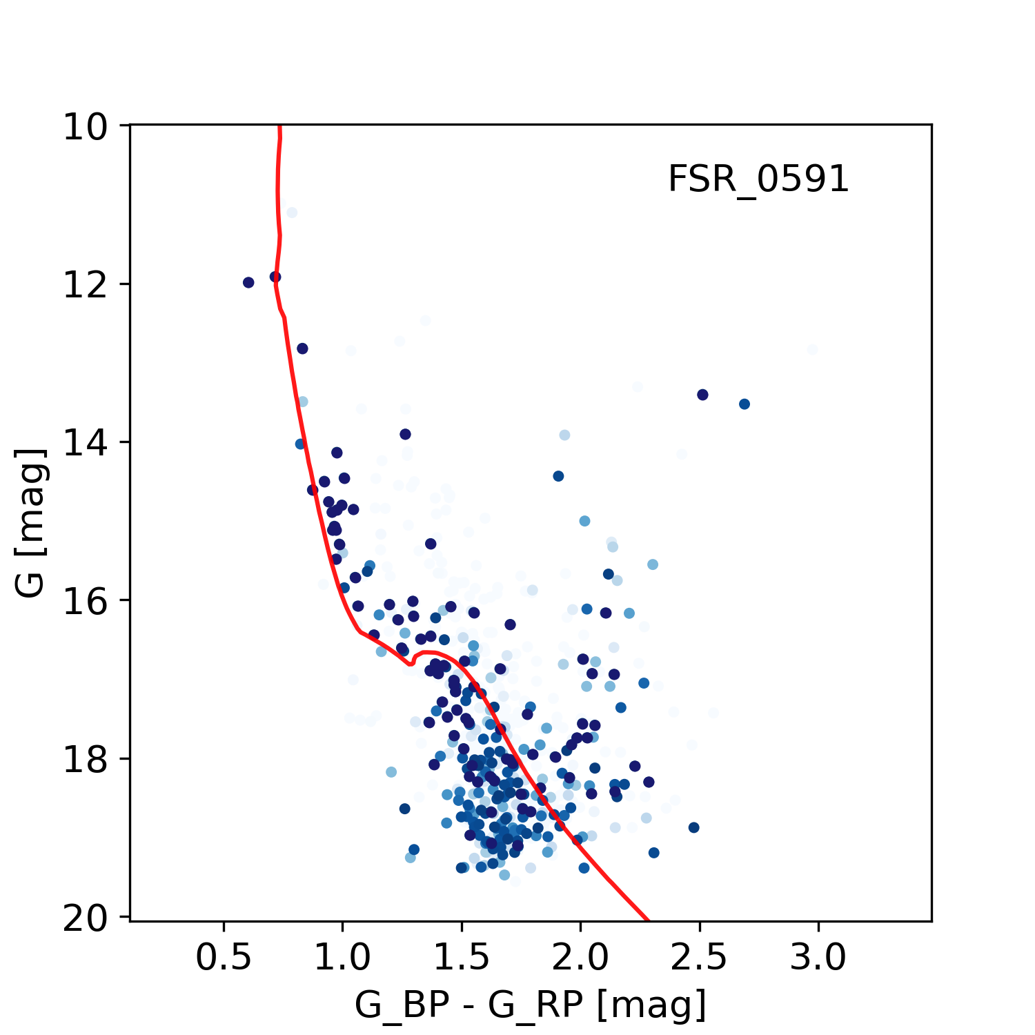
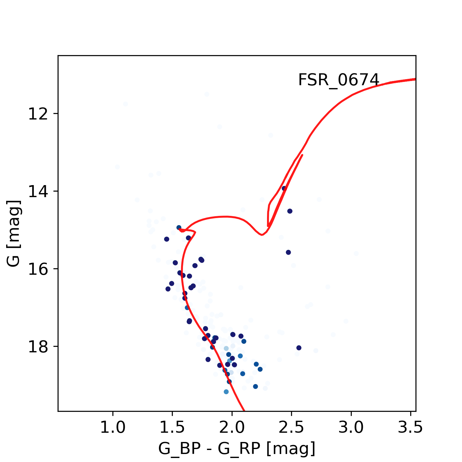
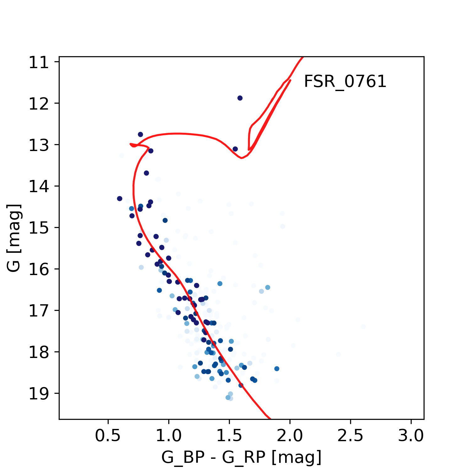
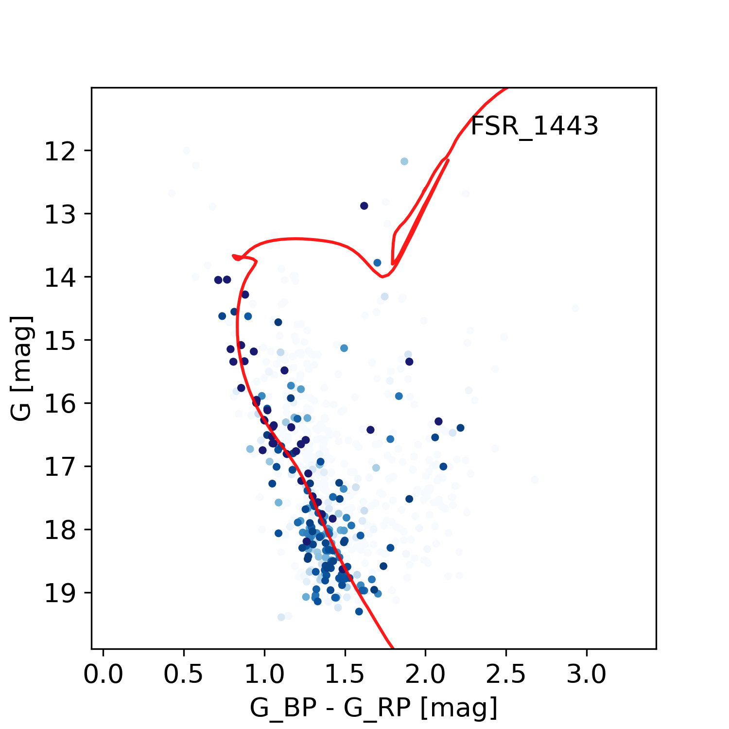
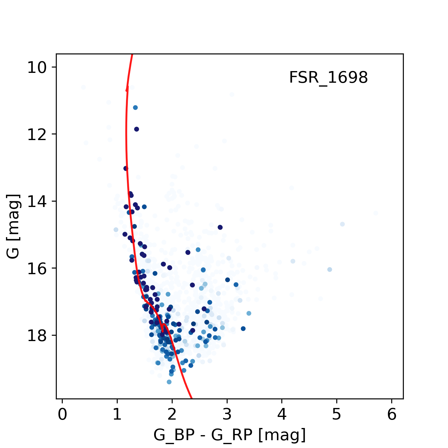
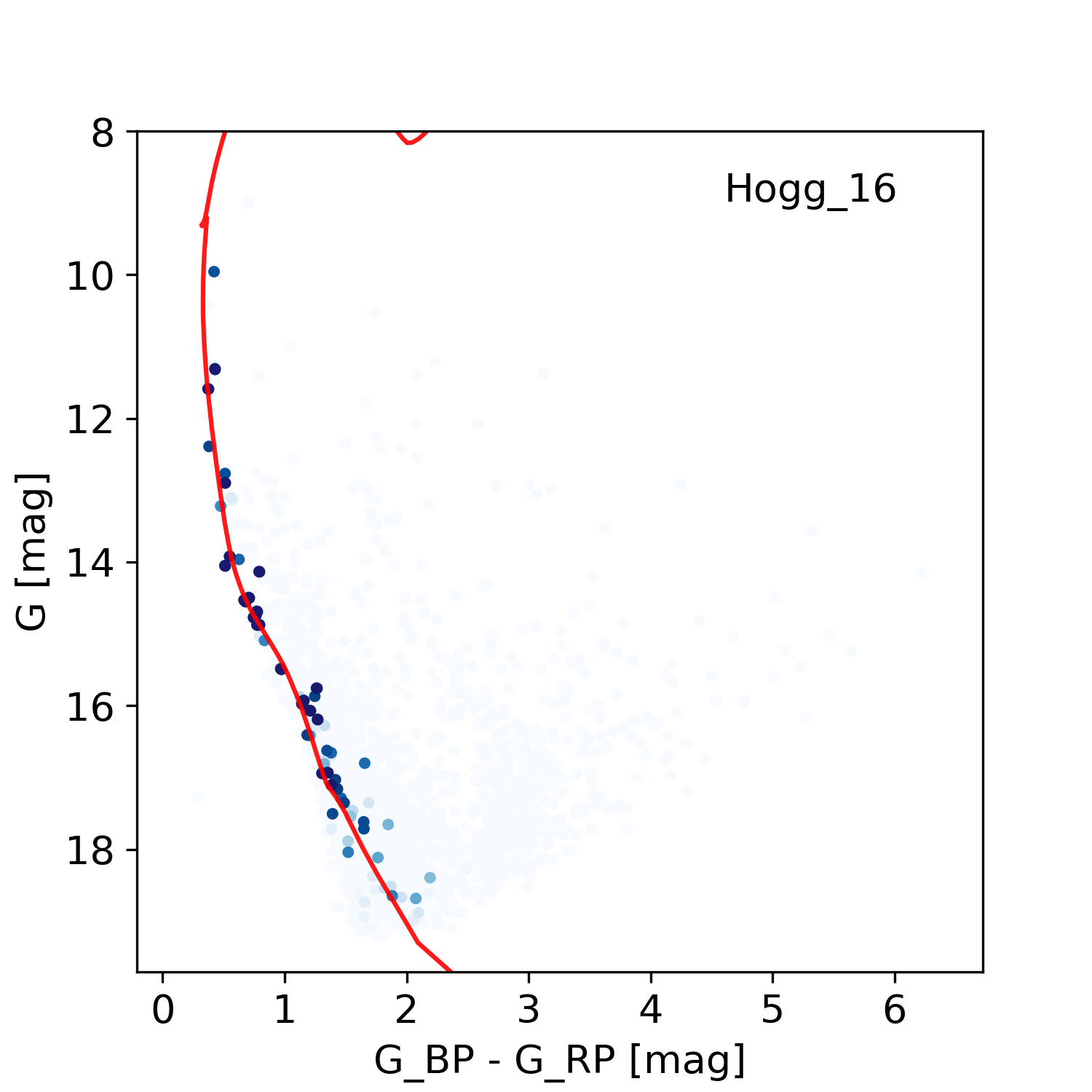
Figure 7: CMDs and isochrone fits (continued)

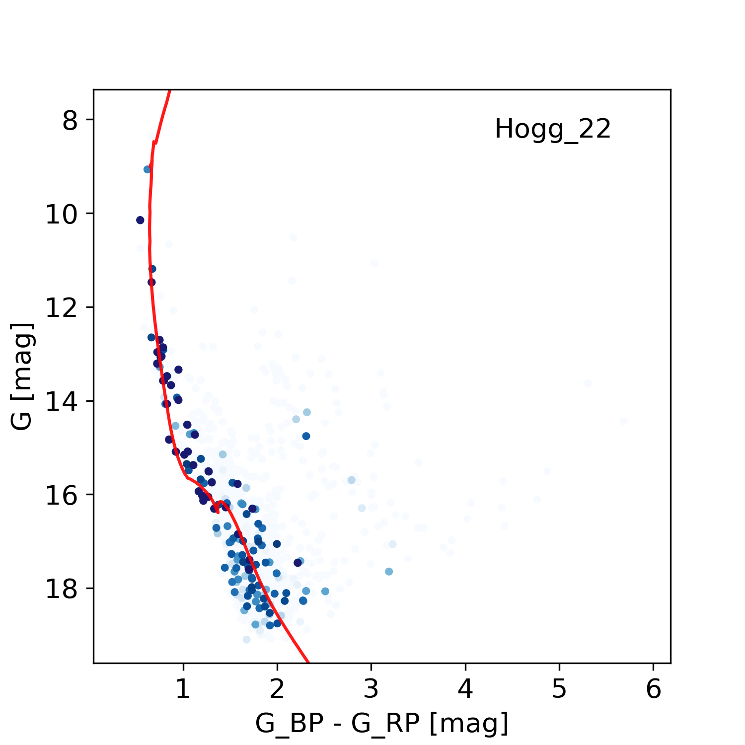
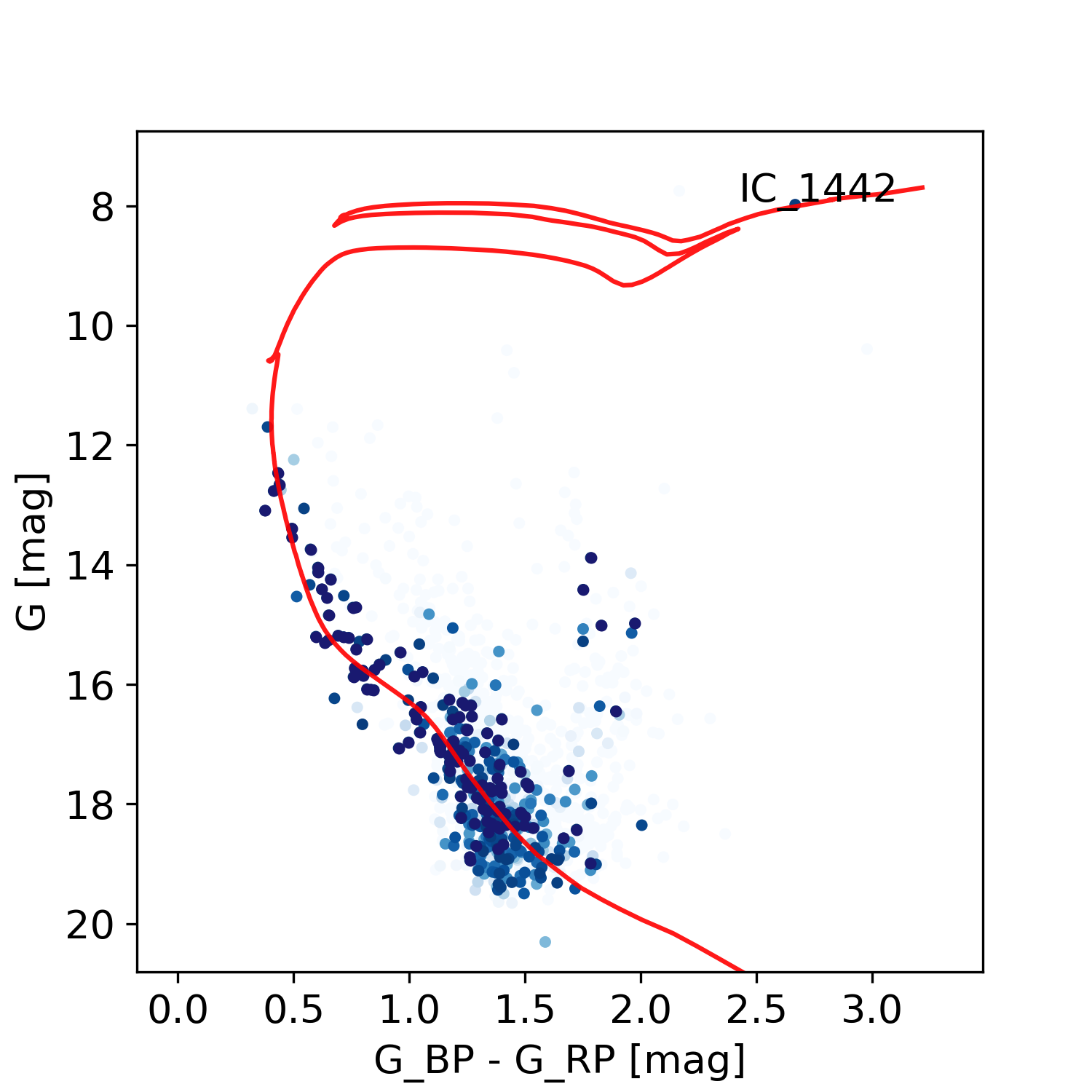
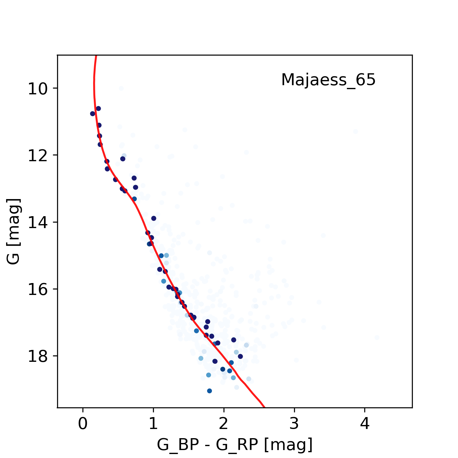
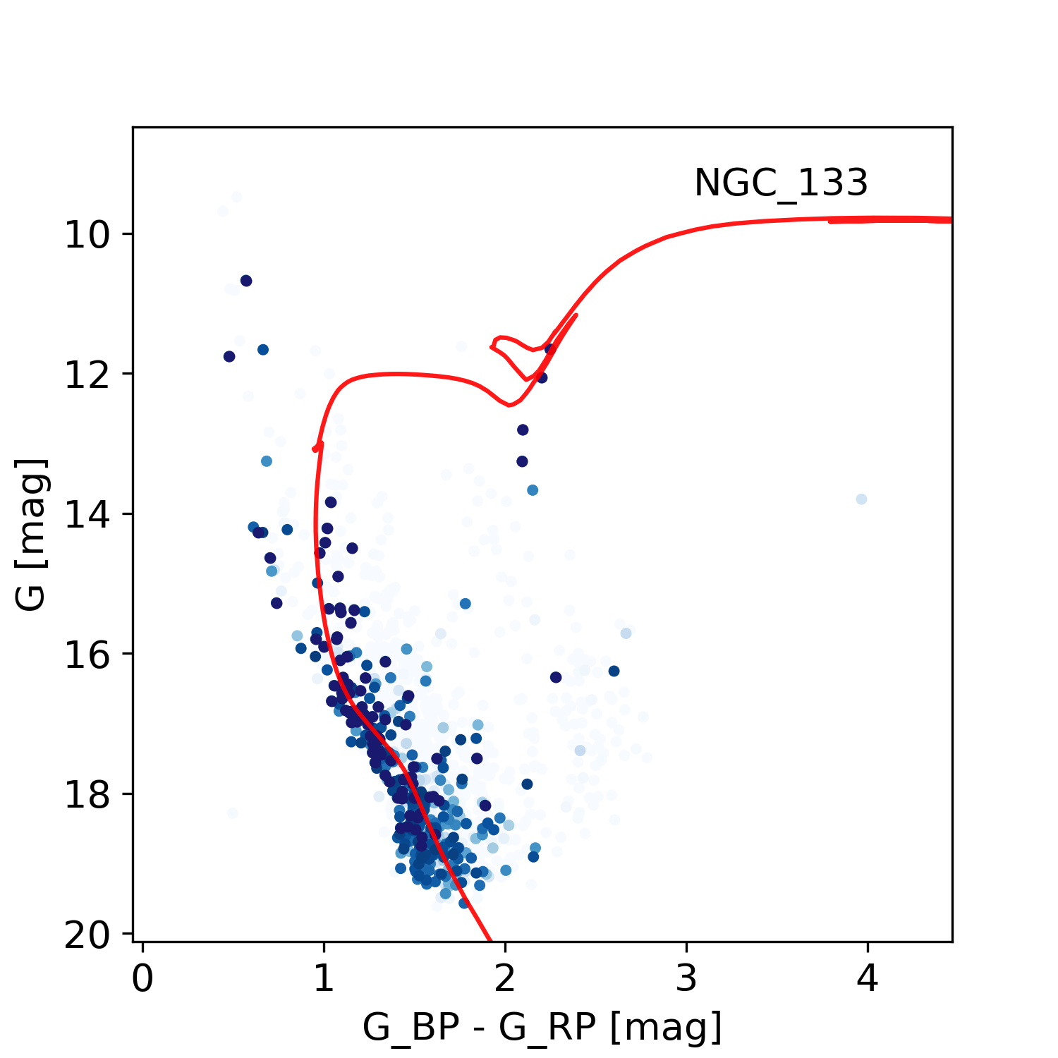
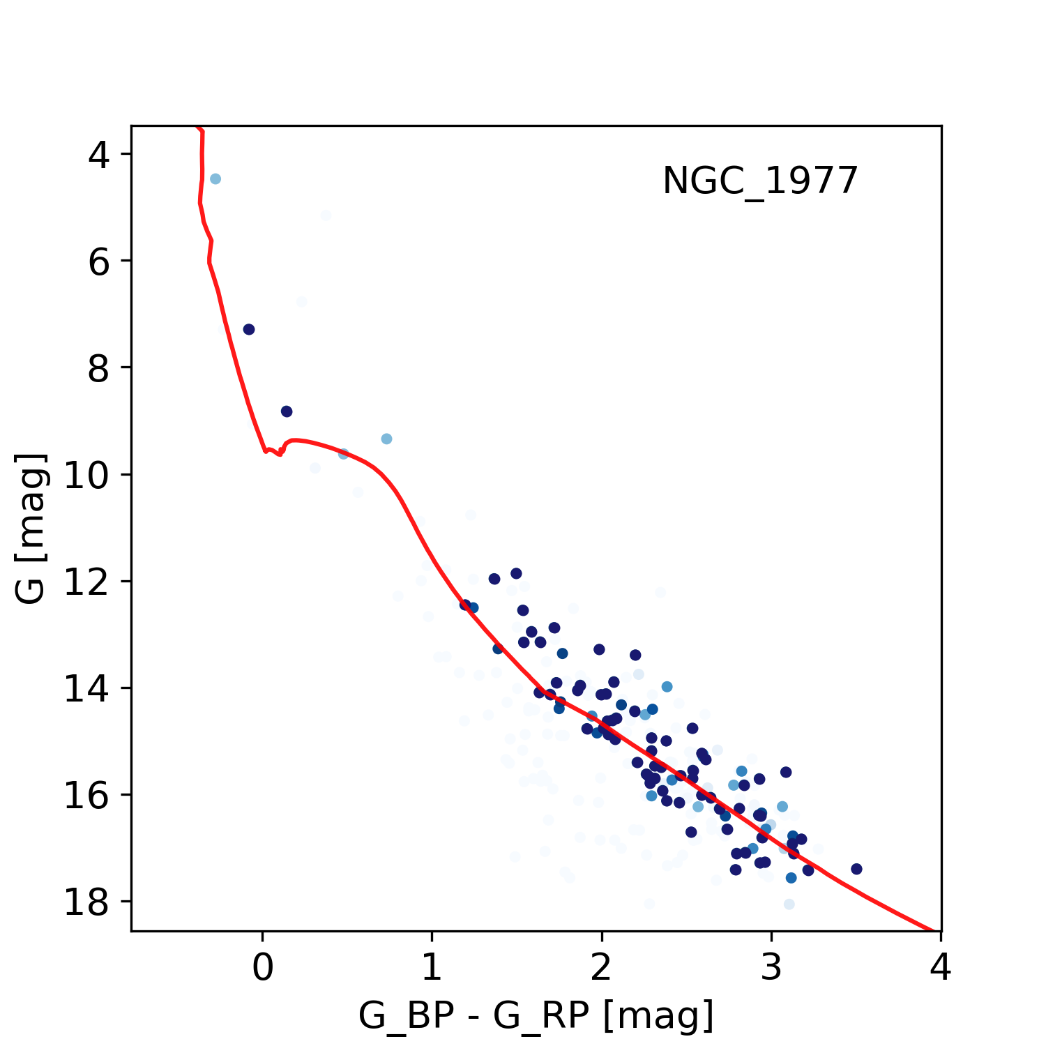
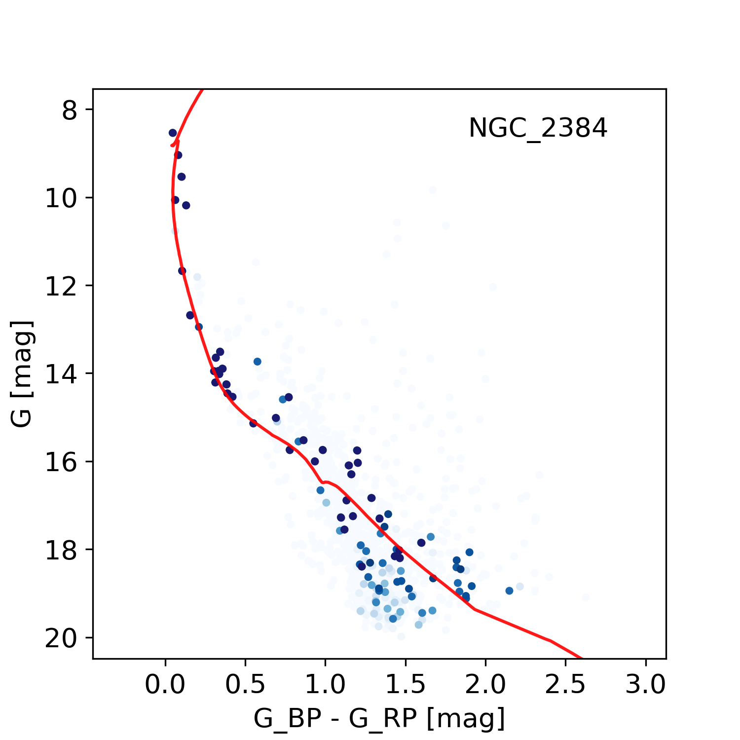
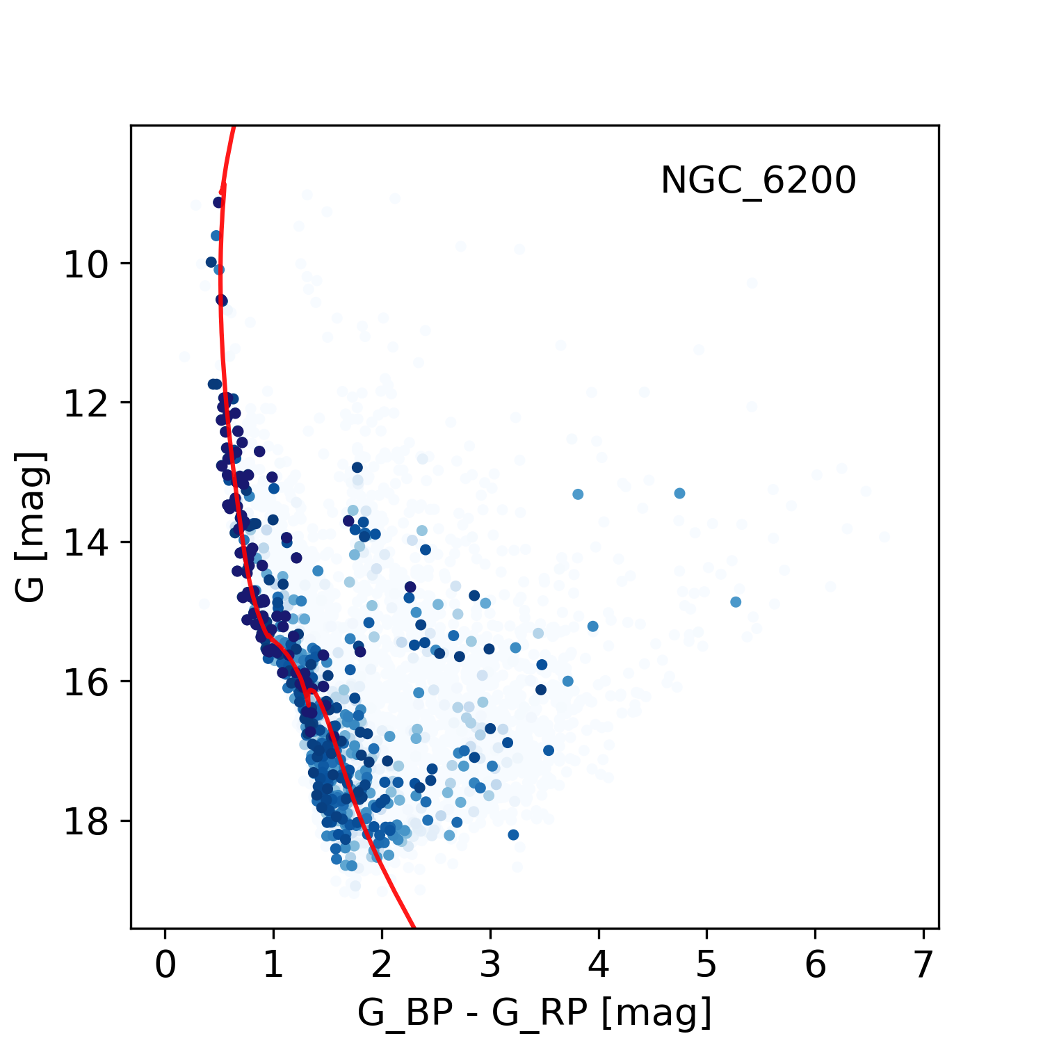
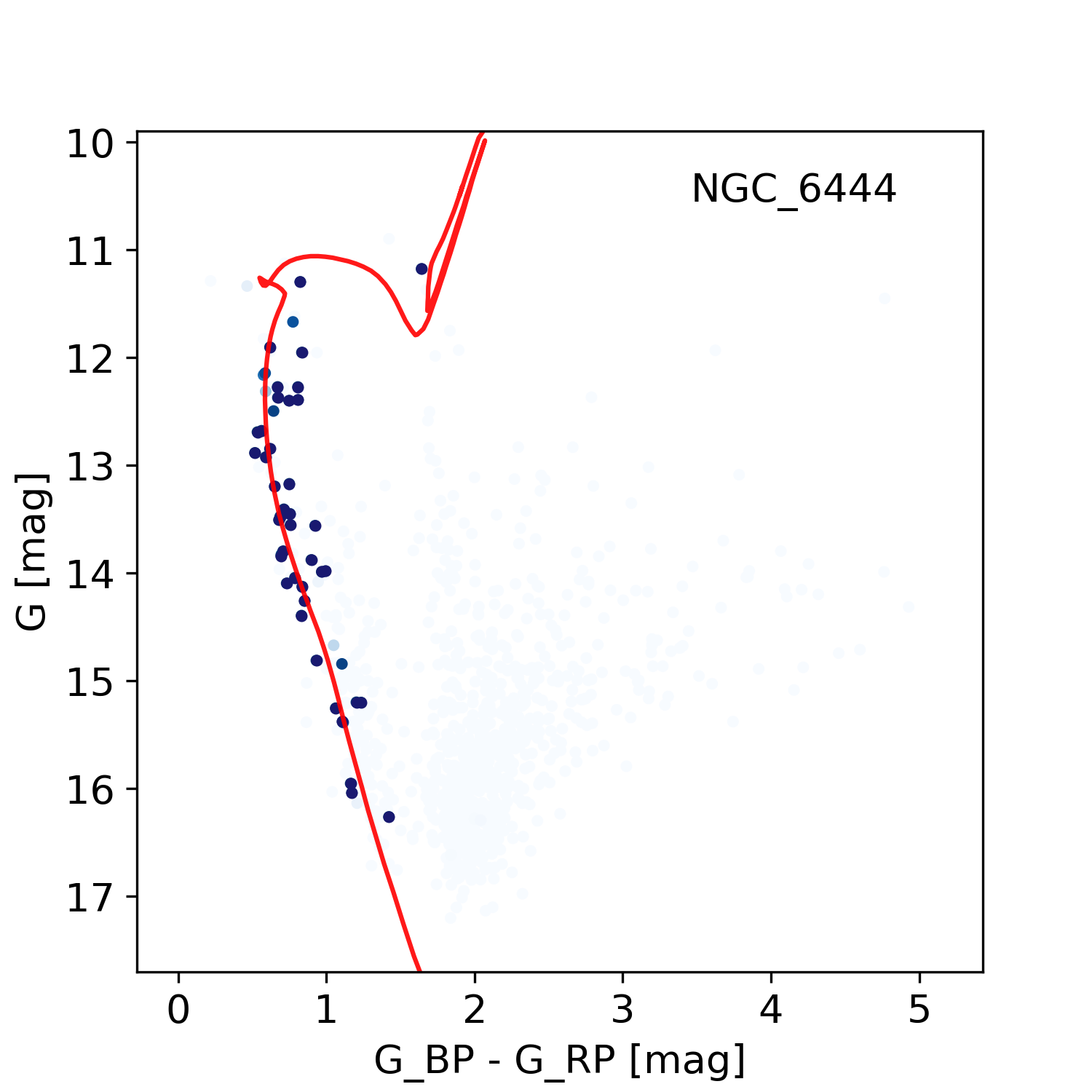
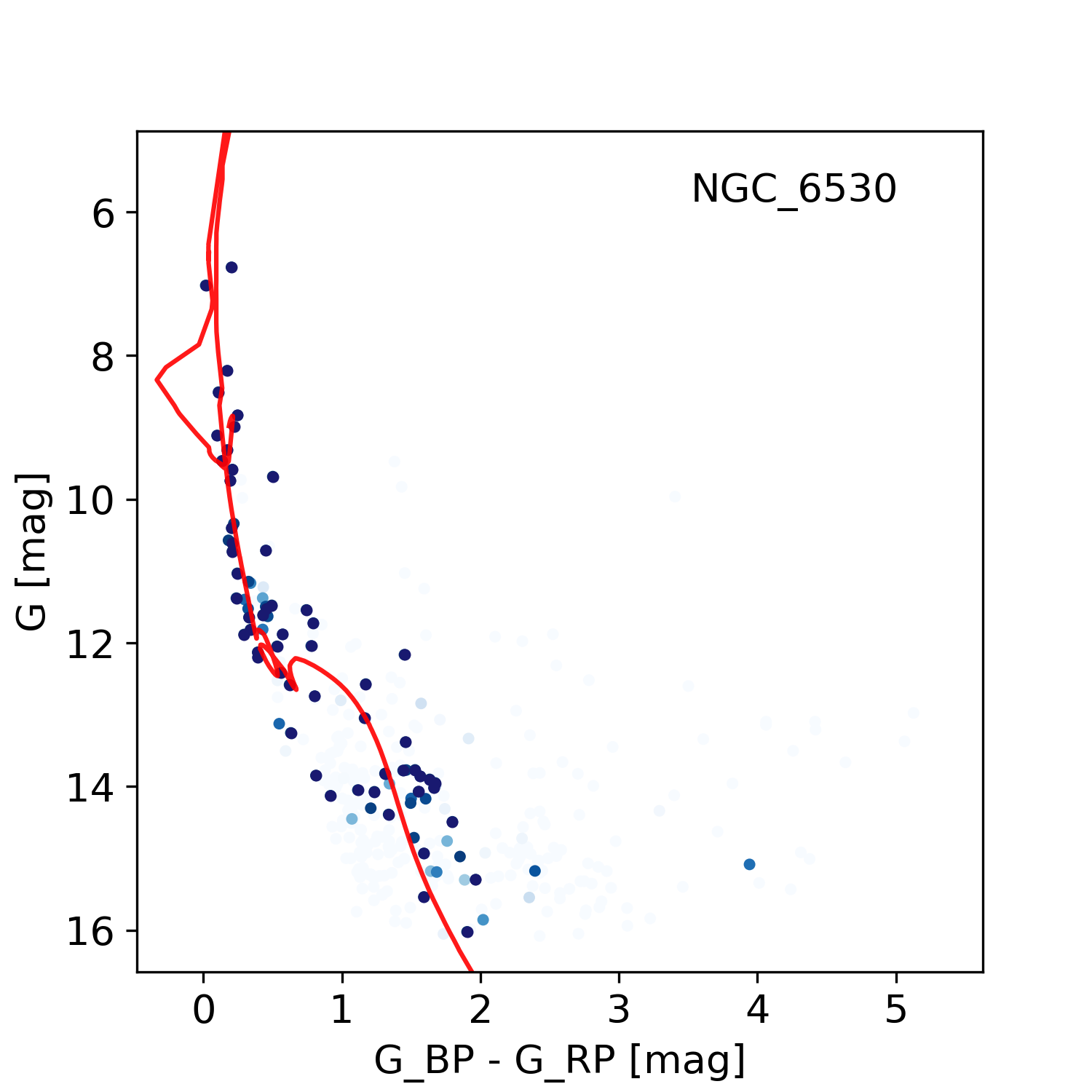
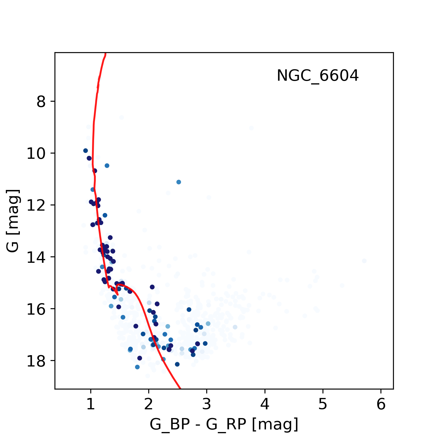
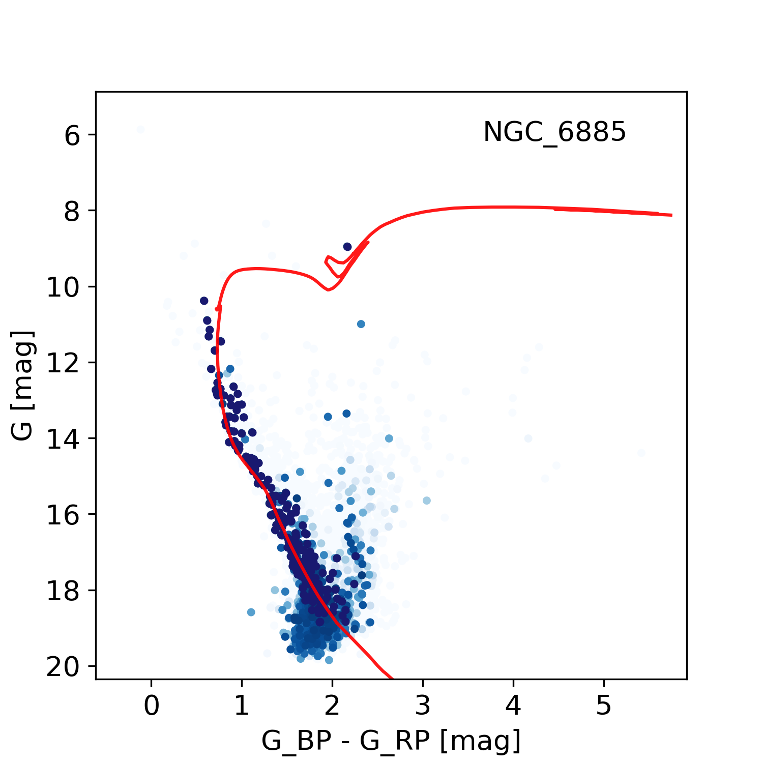
Figure 7: CMDs and isochrone fits (continued)

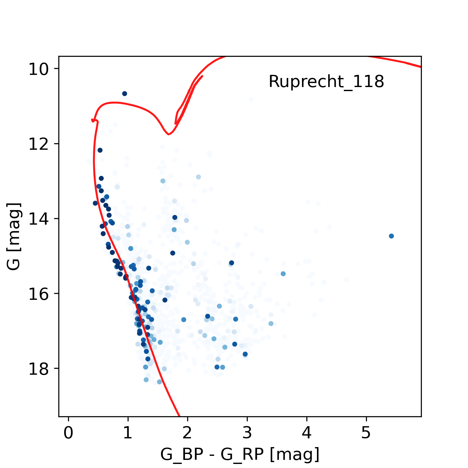
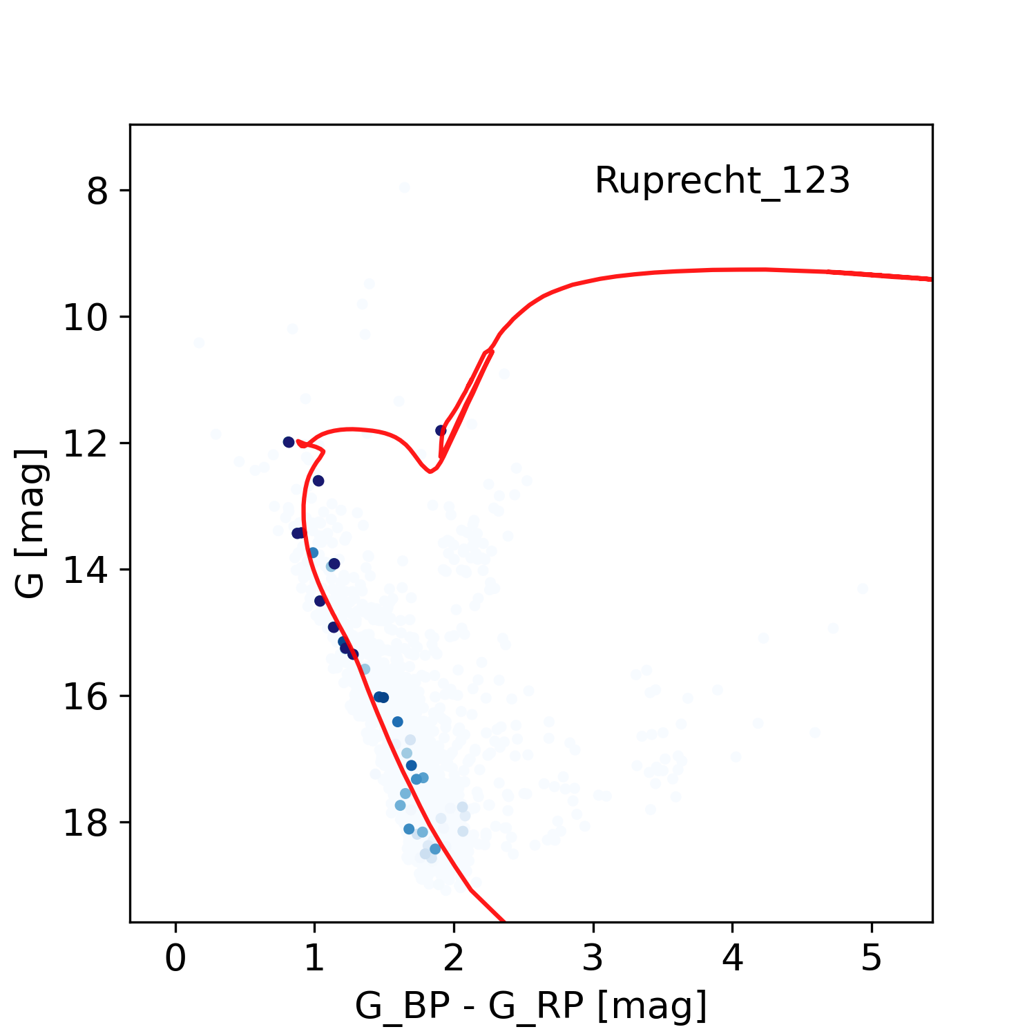
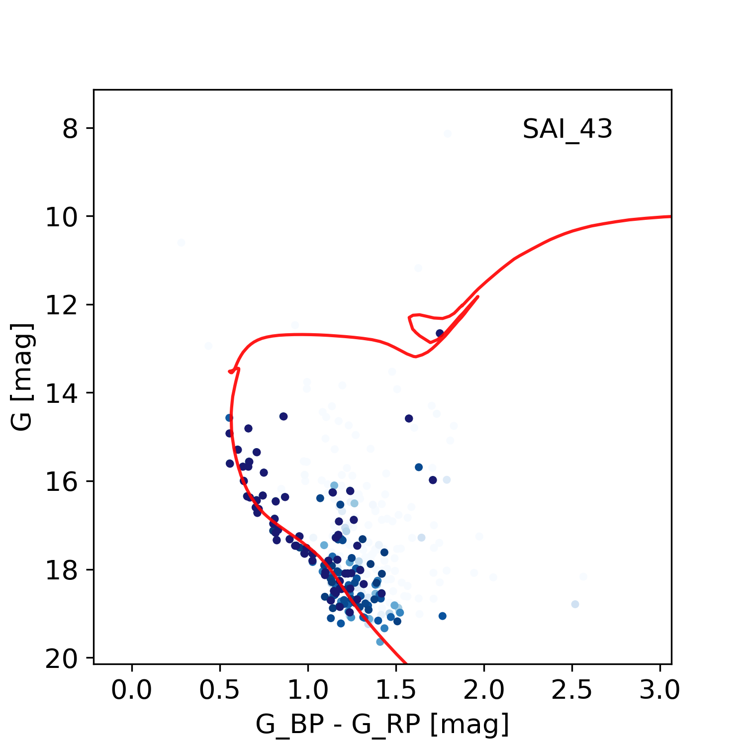
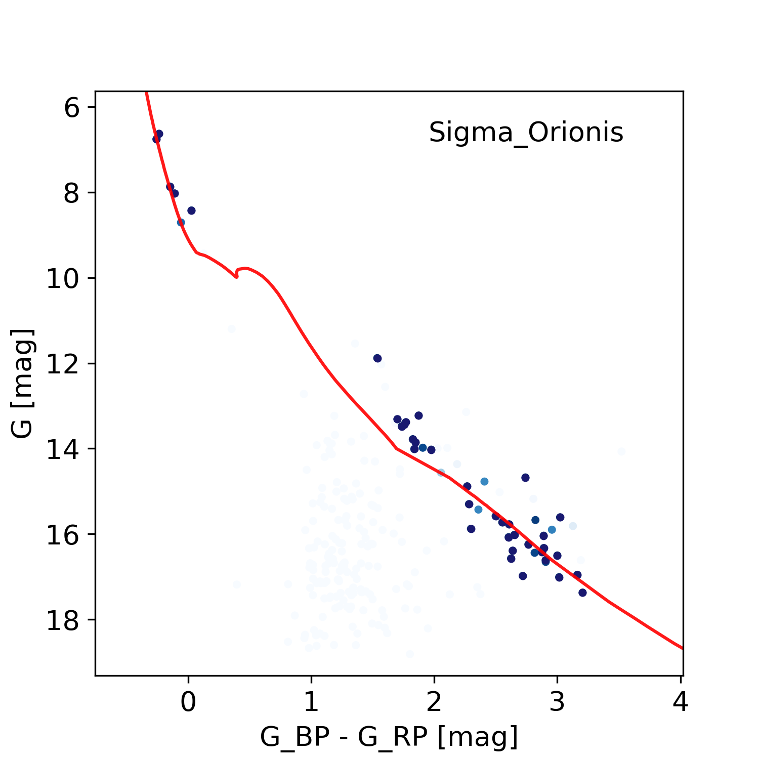
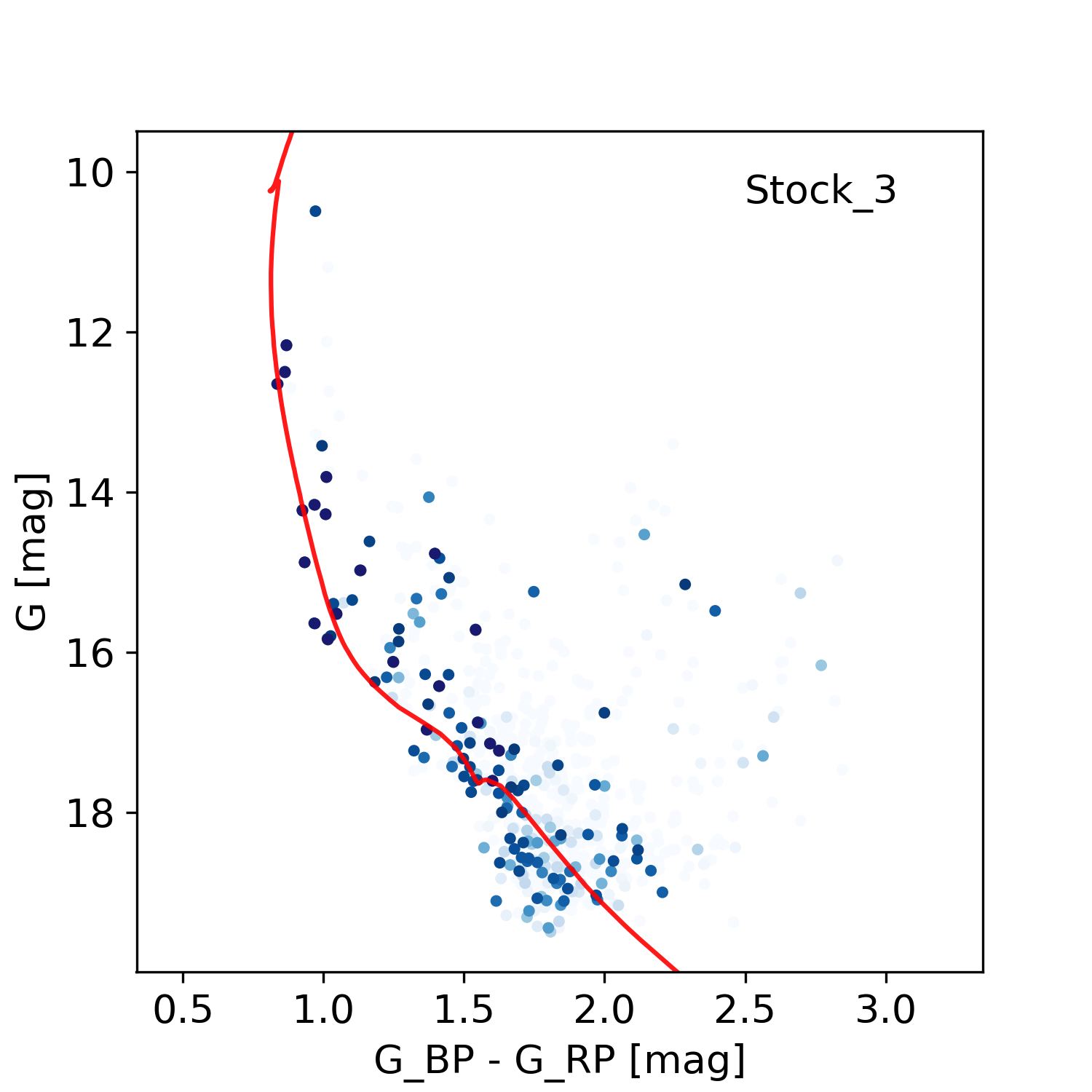
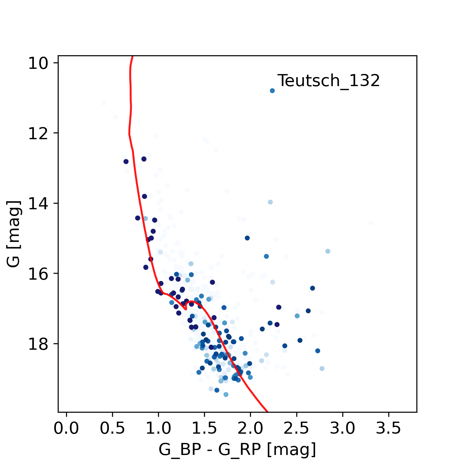
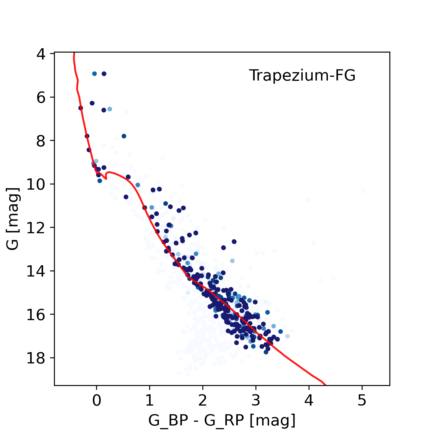
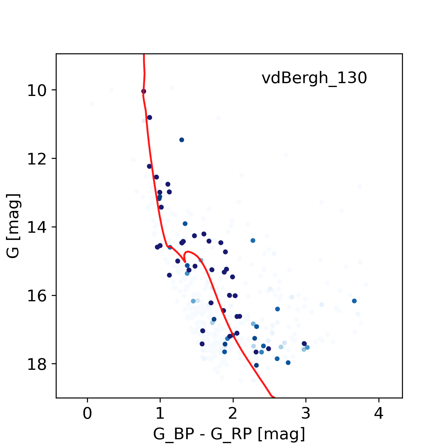
Figure 7: CMDs and isochrone fits (continued)

Data Availability Statement

The data underlying this article, that support the plots and other findings, are available in the article and in its online supplementary material.

This work has made use of data from the European Space Agency(ESA) Gaia (http://www.cosmos.esa.int/gaia) mission, processedby the Gaia Data Processing and Analysis Consortium (DPAC,http://www.cosmos.esa.int/web/gaia/dpac/consortium).

We also employed catalogs from CDS/Simbad (Strasbourg) and Digitized Sky Survey images from the Space Telescope Science Institute (US Government grant NAG W-2166)

Appendix A Results for the high resolution spectroscopy validation sample

Table 4: Results of isochrone fits done using the $[Fe/H]$ prior based on the metallicity gradient from Donor et al. (2020) for the control sample described in section 4.2. The available $[Fe/H]$ values and uncertainties from the literature used in the comparisons are also presented. The h and l suffixes in values from Netopil et al. (2016) denote their high and low quality samples, respectively.

									Carrera et al. (2019)		Netopil et al. (2016)
Name	$dist$	$\sigma_{dist}$	$age$	$\sigma_{age}$	$A_{V}$	$\sigma_{A_{V}}$	$[Fe/H]$	$\sigma_{[Fe/H]}$	$[Fe/H]$	$\sigma_{[Fe/H]}$	$[Fe/H]_{h}$	$\sigma_{[Fe/H]_{h}}$	$[Fe/H]_{l}$	$\sigma_{[Fe/H]_{l}}$
ASCC 21	344	2	7.062	0.039	0.201	0.029	-0.026	0.165	0.01	0.09	-	-	-	-
Basel 11b	1663	71	8.451	0.068	1.856	0.094	-0.090	0.184	0.01	0.05	-	-	-	-
Berkeley 17	3278	105	9.791	0.110	1.923	0.090	-0.173	0.157	-0.10	0.04	-0.06	-	-	-
Berkeley 19	6393	790	9.271	0.042	1.493	0.134	-0.431	0.187	-0.22	-	-	-	-	-
Berkeley 31	7019	329	9.502	0.027	0.540	0.032	-0.302	0.157	-0.31	0.04	-	-	-	-
Berkeley 33	4467	277	8.520	0.051	2.085	0.043	-0.268	0.181	-0.23	0.11	-	-	-0.26	0.05
Berkeley 43	1994	93	7.660	0.338	4.774	0.047	0.171	0.156	0.00	-	-	-	-	-
Berkeley 53	4525	263	8.885	0.021	4.391	0.044	-0.090	0.171	-0.02	0.03	-	-	-	-
Berkeley 66	8738	1318	8.637	0.088	3.886	0.072	-0.110	0.180	-0.12	0.01	-	-	-	-
Berkeley 71	3203	138	8.827	0.030	3.045	0.052	-0.100	0.157	-0.20	0.03	-	-	-	-
Berkeley 9	1720	135	9.187	0.060	2.976	0.037	-0.100	0.198	-0.17	0.18	-	-	-	-
Berkeley 98	3391	78	9.504	0.032	0.753	0.022	-0.090	0.154	0.03	0.02	-	-	-	-
Collinder 69	398	1	6.880	0.043	0.405	0.045	-0.100	0.160	-0.01	0.06	-	-	-	-
Collinder 95	661	8	6.791	0.152	0.886	0.643	-0.065	0.176	-0.03	0.02	-	-	-	-
Czernik 21	3900	510	8.915	0.123	3.211	0.160	-0.268	0.180	-0.24	0.01	-	-	-	-
Czernik 23	3070	172	8.474	0.544	1.761	0.104	-0.100	0.177	-0.25	-	-	-	-	-
Czernik 30	5729	365	9.466	0.023	0.976	0.098	-0.289	0.213	-0.28	0.02	-	-	-	-
FSR 0496	1506	70	8.814	0.023	3.112	0.054	-0.130	0.166	-0.07	-	-	-	-	-
FSR 0542	5506	709	8.889	0.089	3.514	0.107	-0.177	0.290	-0.19	-	-	-	-	-
FSR 0667	1100	28	8.655	0.129	1.502	0.167	0.154	0.227	0.03	0.01	-	-	-	-
FSR 0716	3388	169	9.043	0.051	1.242	0.122	-0.243	0.183	-0.30	-	-	-	-	-
FSR 0941	4029	37	8.826	0.085	2.445	0.057	-0.100	0.225	-0.23	-	-	-	-	-
FSR 0942	3151	510	8.840	0.139	2.414	0.178	-0.122	0.172	-0.28	-	-	-	-	-
Gulliver 6	415	2	7.137	0.079	0.304	0.077	0.031	0.183	-0.10	-	-	-	-	-
Haffner 4	3758	260	8.950	0.118	1.430	0.107	-0.326	0.191	-0.13	-	-	-	-	-
IC 1369	2683	284	7.773	0.695	2.594	0.122	-0.018	0.159	-0.02	0.01	-	-	-	-
IC 1805	1849	113	6.805	0.081	2.296	0.022	-0.056	0.189	0.32	-	-	-	-	-
King 15	2727	140	8.493	0.452	1.926	0.083	-0.100	0.243	-0.05	-	-	-	-	-
Kronberger 57	2211	663	6.738	0.799	4.336	0.148	0.383	0.308	0.02	-	-	-	-	-
Melotte 20	174	3	7.858	0.025	0.386	0.040	0.036	0.162	0.08	0.07	0.14	0.11	-	-
Melotte 22	136	1	8.090	0.097	0.154	0.051	0.127	0.167	0.06	0.08	-0.01	0.05	-	-
Melotte 71	1966	47	9.097	0.031	0.512	0.060	-0.100	0.176	-0.09	0.02	-0.27	-	-	-
NGC 1193	5166	206	9.713	0.057	0.674	0.028	-0.221	0.159	-0.25	0.01	-0.22	-	-	-
NGC 1245	2636	42	9.096	0.016	0.871	0.026	-0.100	0.153	-0.06	0.03	0.02	0.03	-0.05	0.06
NGC 136	4648	282	8.376	0.681	2.124	0.133	-0.124	0.172	-0.22	-	-	-	-	-
NGC 1664	1197	23	8.790	0.022	0.918	0.068	-0.127	0.156	-0.01	-	-	-	-	-
NGC 1798	4741	243	9.139	0.014	1.725	0.086	-0.294	0.191	-0.18	0.02	-	-	-	-
NGC 1817	1544	39	9.078	0.017	0.785	0.067	-0.119	0.166	-0.09	-	-0.11	0.03	-0.16	0.03
NGC 1857	2506	114	8.377	0.398	1.679	0.087	-0.192	0.176	-0.12	-	-	-	-	-
NGC 188	1836	5	9.789	0.018	0.353	0.072	-0.062	0.161	0.13	0.05	0.11	0.04	-0.02	0.09
NGC 1907	1539	54	8.681	0.142	1.672	0.147	-0.268	0.174	-0.05	0.01	-	-	-	-
NGC 1912	1058	22	8.479	0.123	0.937	0.068	0.048	0.164	-0.07	0.02	-0.10	0.14	-	-
NGC 2158	4030	306	9.381	0.065	1.495	0.067	-0.268	0.156	-0.15	0.03	-	-	-0.32	0.08
NGC 2168	845	16	8.145	0.168	0.903	0.077	-0.110	0.173	-0.13	0.07	-	-	-0.21	0.10
NGC 2183	786	34	7.006	0.202	1.670	0.473	-0.100	0.199	-0.08	0.08	-	-	-	-
NGC 2243	4005	106	9.542	0.044	0.168	0.024	-0.358	0.154	-0.42	-	-	-	-0.50	0.08
NGC 2244	1287	107	7.093	0.143	1.586	0.091	-0.121	0.165	-0.23	0.09	-	-	-	-
NGC 2304	3814	143	8.977	0.034	0.308	0.103	-0.275	0.171	-0.09	0.09	-	-	-	-
NGC 2318	1271	41	8.878	0.076	0.839	0.128	0.078	0.158	0.01	-	-	-	-	-
NGC 2324	3732	70	8.749	0.036	0.814	0.073	-0.215	0.156	-0.15	0.05	-0.22	0.07	-	-
NGC 2355	1837	20	9.086	0.034	0.329	0.015	0.042	0.153	-0.11	-	-0.05	0.08	-0.08	0.08
NGC 2420	2471	101	9.407	0.045	0.123	0.009	-0.218	0.158	-0.12	0.03	-0.05	0.02	-0.21	0.09
NGC 2682	855	4	9.561	0.004	0.185	0.030	-0.031	0.154	0.02	0.07	0.03	0.05	0.00	0.06
NGC 6705	1922	50	8.440	0.163	1.502	0.071	0.046	0.16	0.16	0.03	0.12	0.09	0.25	0.05
NGC 6791	4422	74	9.946	0.053	0.391	0.052	0.221	0.165	0.40	0.07	0.42	0.05	0.35	0.07
NGC 6811	1097	17	9.021	0.022	0.232	0.048	0.015	0.161	-0.01	0.04	0.03	0.01	-	-
NGC 6819	2310	141	9.459	0.037	0.507	0.026	0.011	0.166	0.10	0.04	0.09	0.01	-0.04	0.08
NGC 6866	1392	44	8.844	0.034	0.477	0.076	0.183	0.156	0.04	0.02	-	-	-	-
NGC 7058	362	2	7.860	0.584	0.291	0.183	-0.100	0.175	0.12	0.04	-	-	-	-
NGC 7062	2109	168	8.643	0.397	1.730	0.154	-0.081	0.173	0.04	-	-	-	-	-
NGC 752	444	4	9.179	0.019	0.166	0.061	-0.037	0.159	0.01	-	-0.03	0.06	-0.09	0.13
Teutsch 12	3939	331	8.948	0.036	1.969	0.118	-0.118	0.185	-0.14	0.02	-	-	-	-
Teutsch 51	5387	443	8.817	0.068	3.311	0.083	-0.285	0.181	-0.28	0.04	-	-	-	-
Tombaugh 4	3127	215	8.918	0.062	3.218	0.065	-0.103	0.154	-0.47	-	-	-	-	-
Trumpler 26	1336	76	8.669	0.114	1.703	0.108	0.175	0.172	0.28	0.05	-	-	-	-
Trumpler 3	663	8	8.094	0.079	0.931	0.042	0.156	0.150	-0.22	-	-	-	-	-
Trumpler 5	3275	56	9.536	0.025	1.846	0.066	-0.152	0.164	-0.36	0.02	-0.44	0.07	-0.47	0.05

Appendix B Removed clusters

Here we identify the clusters that have been removed from our studied sample, as discussed in section 5.

Table 5: Removed clusters. Central coordinates and radii from DAML.

Name	$RA_{J2000}$	$DE_{J2000}$	$radius$
	$(deg)$	$(deg)$	$(deg)$
ASCC 94	273.9000	-14.9900	0.250
BH 4	114.4333	-36.0667	0.017
Bochum 1	96.3542	19.7667	0.217
Collinder 347	266.5750	-29.3333	0.083
Collinder 92	95.7250	5.1167	0.092
Dolidze 13	12.4250	64.1264	0.133
Dolidze 24	101.1708	1.6847	0.157
Dolidze 35	291.3500	11.6583	0.058
Dolidze 41	304.7042	37.7500	0.092
Dolidze 49	101.7667	-0.0069	0.018
ESO 522 05	273.2208	-24.3639	0.037
FSR 0182	297.9417	33.5119	0.010
FSR 0258	311.2083	43.9150	0.013
FSR 0354	332.8000	57.6994	0.043
FSR 0453	356.8542	63.2264	0.037
FSR 0522	13.4583	65.7933	0.006
FSR 0717	71.5250	42.1342	0.018
FSR 0891	94.3708	22.4272	0.012
FSR 0929	96.3833	17.7200	0.007
FSR 1535	151.9792	-59.1969	0.018
Hogg 11	167.9042	-60.4000	0.017
Kronberger 39	163.5583	-61.7378	0.007
Majaess 50	71.3625	41.9758	0.142
Majaess 95	124.4708	-35.8800	0.025
NGC 2013	86.0042	55.7933	0.050
Patchick 78	8.2917	65.1167	0.013
Ruprecht 120	248.7917	-48.2833	0.025
Ruprecht 136	269.8250	-24.7000	0.025
Ruprecht 59	124.8375	-34.4833	0.025
Teutsch 64	128.1292	-41.9881	0.038

References

- Alves & Bouy (2012) Alves J., Bouy H., 2012, A&A, 547, A97
- Becker & Fenkart (1970) Becker W., Fenkart R. B., 1970, in Becker W., Kontopoulos G. I., eds, IAU Symposium Vol. 38, The Spiral Structure of our Galaxy. p. 205
- Bossini et al. (2019) Bossini D., et al., 2019, A&A, 623, A108
- Bressan et al. (2012) Bressan A., Marigo P., Girardi L., Salasnich B., Dal Cero C., Rubele S., Nanni A., 2012, MNRAS, 427, 127
- Cantat-Gaudin & Anders (2020) Cantat-Gaudin T., Anders F., 2020, A&A, 633, A99
- Cantat-Gaudin et al. (2018) Cantat-Gaudin T., et al., 2018, A&A, 618, A93
- Cantat-Gaudin et al. (2020) Cantat-Gaudin T., et al., 2020, A&A, 640, A1
- Capitanio et al. (2017) Capitanio L., Lallement R., Vergely J. L., Elyajouri M., Monreal-Ibero A., 2017, A&A, 606, A65
- Carraro (2002) Carraro G., 2002, A&A, 387, 479
- Carrera et al. (2019) Carrera R., et al., 2019, A&A, 623, A80
- Castelli & Kurucz (2003) Castelli F., Kurucz R. L., 2003, in Piskunov N., Weiss W. W., Gray D. F., eds, IAU Symposium Vol. 210, Modelling of Stellar Atmospheres. p. A20 (arXiv:astro-ph/0405087)
- Castro-Ginard et al. (2020) Castro-Ginard A., et al., 2020, A&A, 635, A45
- Chen et al. (2019) Chen B., D’Onghia E., Alves J., Adamo A., 2019, arXiv e-prints, p. arXiv:1905.11429
- Danielski et al. (2018) Danielski C., Babusiaux C., Ruiz-Dern L., Sartoretti P., Arenou F., 2018, A&A, 614, A19
- Dias et al. (2002) Dias W. S., Alessi B. S., Moitinho A., Lépine J. R. D., 2002, A&A, 389, 871
- Dias et al. (2014) Dias W. S., Monteiro H., Caetano T. C., Lépine J. R. D., Assafin M., Oliveira A. F., 2014, A&A, 564, A79
- Dias et al. (2018) Dias W. S., Monteiro H., Lépine J. R. D., Prates R., Gneiding C. D., Sacchi M., 2018, MNRAS, 481, 3887
- Dias et al. (2019) Dias W. S., Monteiro H., Lépine J. R. D., Barros D. A., 2019, MNRAS, 486, 5726
- Donor et al. (2020) Donor J., et al., 2020, AJ, 159, 199
- Fitzpatrick et al. (2019) Fitzpatrick E. L., Massa D., Gordon K. D., Bohlin R., Clayton G. C., 2019, ApJ, 886, 108
- Gaia Collaboration et al. (2016) Gaia Collaboration et al., 2016, A&A, 595, A1
- Gaia Collaboration et al. (2018a) Gaia Collaboration et al., 2018a, A&A, 616, A1
- Gaia Collaboration et al. (2018b) Gaia Collaboration et al., 2018b, A&A, 616, A10
- Janes & Adler (1982) Janes K., Adler D., 1982, ApJS, 49, 425
- Kharchenko et al. (2005) Kharchenko N. V., Piskunov A. E., Röser S., Schilbach E., Scholz R. D., 2005, A&A, 438, 1163
- Kharchenko et al. (2013) Kharchenko N. V., Piskunov A. E., Schilbach E., Röser S., Scholz R.-D., 2013, A&A, 558, A53
- Kounkel & Covey (2019) Kounkel M., Covey K., 2019, AJ, 158, 122
- Krone-Martins & Moitinho (2014) Krone-Martins A., Moitinho A., 2014, A&A, 561, A57
- Lindegren et al. (2018) Lindegren L., et al., 2018, A&A, 616, A2
- Liu & Pang (2019) Liu L., Pang X., 2019, ApJS, 245, 32
- Luri et al. (2018) Luri X., et al., 2018, A&A, 616, A9
- Lyngå (1988) Lyngå G., 1988, in European Southern Observatory Conference and Workshop Proceedings. pp 379–382
- Lyra et al. (2006) Lyra W., Moitinho A., van der Bliek N. S., Alves J., 2006, A&A, 453, 101
- Maíz Apellániz & Weiler (2018) Maíz Apellániz J., Weiler M., 2018, A&A, 619, A180
- Maurya et al. (2020) Maurya J., Joshi Y. C., Gour A. S., 2020, arXiv e-prints, p. arXiv:2005.07375
- Moitinho (2010) Moitinho A., 2010, in de Grijs R., Lépine J. R. D., eds, IAU Symposium Vol. 266, Star Clusters: Basic Galactic Building Blocks Throughout Time and Space. pp 106–116 (arXiv:0911.1459), doi:10.1017/S1743921309990949
- Monteiro & Dias (2019) Monteiro H., Dias W. S., 2019, MNRAS, 487, 2385
- Monteiro et al. (2017) Monteiro H., Dias W. S., Hickel G. R., Caetano T. C., 2017, New Astron., 51, 15
- Netopil et al. (2015) Netopil M., Paunzen E., Carraro G., 2015, A&A, 582, A19
- Netopil et al. (2016) Netopil M., Paunzen E., Heiter U., Soubiran C., 2016, A&A, 585, A150
- Pavani & Bica (2007) Pavani D. B., Bica E., 2007, A&A, 468, 139
- Perren et al. (2020) Perren G. I., Giorgi E. E., Moitinho A., Carraro G., Pera M. S., Vázquez R. A., 2020, A&A, 637, A95
- Roeser et al. (2010) Roeser S., Demleitner M., Schilbach E., 2010, AJ, 139, 2440
- Sim et al. (2019) Sim G., Lee S. H., Ann H. B., Kim S., 2019, Journal of Korean Astronomical Society, 52, 145
- Skrutskie et al. (2006) Skrutskie M. F., et al., 2006, AJ, 131, 1163
- Soubiran et al. (2018) Soubiran C., et al., 2018, A&A, 619, A155
- The Astropy Collaboration et al. (2018) The Astropy Collaboration et al., 2018, AJ, 156, 123
- Wang & Chen (2019) Wang S., Chen X., 2019, ApJ, 877, 116