Abstract

In randomized clinical trials, adjustments for baseline covariates at both design and analysis stages are highly encouraged by regulatory agencies. A recent trend is to use a model-assisted approach for covariate adjustment to gain credibility and efficiency while producing asymptotically valid inference even when the model is incorrect. In this article we present three considerations for better practice when model-assisted inference is applied to adjust for covariates under simple or covariate-adaptive randomized trials: (1) guaranteed efficiency gain: a model-assisted method should often gain but never hurt efficiency; (2) wide applicability: a valid procedure should be applicable, and preferably universally applicable, to all commonly used randomization schemes; (3) robust standard error: variance estimation should be robust to model misspecification and heteroscedasticity. To achieve these, we recommend a model-assisted estimator under an analysis of heterogeneous covariance working model including all covariates utilized in randomization. Our conclusions are based on an asymptotic theory that provides a clear picture of how covariate-adaptive randomization and regression adjustment alter statistical efficiency. Our theory is more general than the existing ones in terms of studying arbitrary functions of response means (including linear contrasts, ratios, and odds ratios), multiple arms, guaranteed efficiency gain, optimality, and universal applicability.

Keywords: Analysis of covariance; Covariate-adaptive randomization; Efficiency; Heteroscedasticity; Model-assisted; Multiple treatment arms; Treatment-by-covariate interaction.

1 Introduction

Consider a clinical trial with patients randomized into one and only one of multiple treatment arms according to fixed assignment proportions. Each patient has multiple potential responses, one for each treatment, but only one response is observed depending on the assigned treatment. Based on data collected from the trial, we would like to make statistical inference on treatment effects defined as functions of the response means (e.g., linear contrasts, ratios, or odds ratios). These unconditional treatment effects are discussed in a recent Food and Drug Administration draft guidance (FDA,, 2021).

In clinical trials, we typically observe some baseline covariates for each patient, which are measured prior to treatment assignments and, hence, are not affected by the treatment. As emphasized in regulatory agency guidelines, baseline covariates are encouraged to be utilized in the following two ways. (i) In the design stage, covariate-adaptive randomization can be used to enforce the balance of treatment assignments across levels of discrete baseline prognostic factors, such as institution, disease stage, prior treatment, gender, and age group. “Balance of treatment groups with respect to one or more specific prognostic covariates can enhance the credibility of the results of the trial” (EMA,, 2015, European Medicines Agency). (ii) In the analysis stage, baseline covariates can be used to gain efficiency. “Incorporating prognostic baseline factors in the primary statistical analysis of clinical trial data can result in a more efficient use of data to demonstrate and quantify the effects of treatment with minimal impact on bias or the Type I error rate” (FDA,, 2021). More specifically, the investigator is advised to “identify those covariates and factors expected to have an important influence on the primary variable(s)” and to specify “how to account for them in the analysis in order to improve precision and to compensate for any lack of balance between groups” (ICH E9,, 1998).

For efficiency gain, one may apply a model-based approach using a model between the potential responses and covariates. However, the validity of a model-based approach requires a correct model specification, i.e., a possibly strong assumption. As emphasized in FDA, (2021), a method used for covariate adjustment “should provide valid inference under approximately the same minimal statistical assumptions that would be needed for unadjusted estimation in a randomized trial”. Consequently, model-assisted approaches, which gain efficiency through a working model between responses and covariates and still produce asymptotically valid inference even when the working model is misspecified, have become considerably more popular.

1.1 Considerations about covariate adjustment

For better practice of covariate adjustment via model-assisted approaches, we present the following three considerations.

1. Guaranteed efficiency gain. The working model should be chosen so that the resulting model-assisted estimator often gains but never loses efficiency when compared to a benchmark estimator that does not adjust for any covariate.

This consideration is important for model-assisted inference because covariate adjustment based on a misspecified working model does not necessarily lead to efficiency gain over the benchmark. One example is the customary analysis of covariance (ANCOVA) whose working model does not include treatment-by-covariate interaction terms, which we refer to as the homogeneous working model (§2.3). These interaction terms are often ignored or even discouraged in practice because of two perceptions: (i) even if the homogeneous working model is misspecified, ANCOVA still provides valid inference as it is model-assisted; (ii) a model without interaction terms have fewer coefficients to estimate and may have better finite sample properties. These perceptions are correct but only provide a partial picture. When the treatment effect is indeed heterogeneous, the ANCOVA estimator using the homogeneous working model may be even less efficient than the benchmark analysis of variance (ANOVA) estimator that uses no model assistance at all (Freedman, 2008a, ; Lin,, 2013). This has led to confusion about how covariate adjustment should be implemented, which can be seen from conflicting recommendations by regulatory agencies: “The primary model should not include treatment by covariate interactions.” (EMA,, 2015); “The linear models may include treatment by covariate interaction terms.” (FDA,, 2021).

Is there a model-assisted method that achieves guaranteed efficiency gain? An affirmative answer is provided in §1.2.

2. Wide applicability. The model-assisted inference procedure should be applicable to all commonly used randomization schemes.

Covariate-adaptive randomization has been widely used in modern clinical trials to balance treatments across important prognostic factors. According to a recent review of nearly 300 clinical trials published in 2009 and 2014, 237 of them used covariate-adaptive randomization (Ciolino et al.,, 2019). The three most popular covariate-adaptive randomization schemes are the stratified permuted block (Zelen,, 1974), the stratified biased coin (Shao et al.,, 2010; Kuznetsova and Johnson,, 2017), and Pocock-Simon’s minimization (Taves,, 1974; Pocock and Simon,, 1975; Han et al.,, 2009). Unlike simple randomization, covariate-adaptive randomization generates a dependent sequence of treatment assignments. As recognized by regulatory agencies (EMA,, 2015; FDA,, 2021), conventional inference procedures developed under simple randomization are not necessarily valid under covariate-adaptive randomization. Thus, the second consideration is whether the model-assisted inference procedure is applicable to all commonly used randomization schemes.

3. Robust standard error. The model-assisted inference should use standard errors robust against model misspecification and heteroscedasticity.

The use of robust standard error is a crucial step for valid model-assisted inference (FDA,, 2021). Although the asymptotic theory for heteroscedasticity-robust standard errors was developed decades ago (Huber,, 1967; White,, 1980) and has been widely used in econometrics, its usage in clinical trials is scarce.

1.2 Our contributions

Given how frequently covariate adjustment is being used in practice, it may come as a surprise that there has been no comprehensive guideline yet. In our opinion, this is because most existing papers consider some aspects but not a full picture regarding the three considerations described in §1.1. For example, most existing results are for linear contrasts of response means for two arms (Yang and Tsiatis,, 2001; Tsiatis et al.,, 2008; Shao et al.,, 2010; Lin,, 2013; Shao and Yu,, 2013; Ma et al.,, 2015; Bugni et al.,, 2018; Ye,, 2018; Wang et al., 2019a, ; Wang et al., 2019b, ; Liu and Yang,, 2020; Ma et al., 2020a, ; Ma et al., 2020b, , among others); many of them are applicable to only simple randomization or a limited class of randomization schemes with well-understood properties; Bugni et al., (2019) and Ye et al., (2020) consider multiple arms but still focus on linear contrasts and do not fully address the guaranteed efficiency gain or optimality; not enough insights are provided to convince practitioners to apply model-assisted inference.

We establish a comprehensive theory to provide a clear picture of how covariate-adaptive randomization and regression adjustment alter statistical efficiency, which resolves some confusion about covariate adjustment and facilitates its better practice with easy-to-implement recommendation for practitioners. Our theory is more general than the existing ones in terms of studying arbitrary functions of response means (including linear contrasts, ratios and odds ratios), multiple arms, guaranteed efficiency gain, optimality, and universal applicability.

Our theory shows that a heterogeneous working model for ANCOVA that includes all treatment-by-covariate interaction terms should be favored because it achieves both guaranteed efficiency gain and wide applicability when all covariates utilized in covariate-adaptive randomization are included in the working model. To distinguish from the customary ANCOVA that uses a homogeneous working model, we term the ANCOVA using a heterogeneous working model as ANalysis of HEterogeneous COVAriance (ANHECOVA). Note that ANHECOVA is not a new proposal and has a long history in the literature with a recent resurgence of attention (Cassel et al.,, 1976; Yang and Tsiatis,, 2001; Tsiatis et al.,, 2008; Lin,, 2013; Wang et al., 2019a, ; Liu and Yang,, 2020; Li and Ding,, 2020, among others), but our recommendation of ANHECOVA is from a more comprehensive perspective. Specifically, in §3.2-§3.3, we show that under mild and transparent assumptions, the recommended ANHECOVA estimator of the response mean vector is consistent, asymptotically normal, and asymptotically more efficient than the benchmark ANOVA or ANCOVA estimator; in fact, the ANHECOVA estimator is asymptotically the most efficient estimator within a class of linearly-adjusted estimators. Special cases of this result have been discussed in the literature, but our development is for a much more general setting that considers multiple treatment arms, joint estimation of response means, and under all commonly used covariate-adaptive randomization schemes. In §3.1 we offer explanations of why the heterogeneous working model is generally preferable over the homogeneous working model.

Besides guaranteed efficiency gain and wide applicability, our asymptotic theory in §3.2-3.3 shows that the recommended ANHECOVA procedure also enjoys a universality property, i.e., the same inference procedure can be universally applied to all commonly used randomization schemes including Pocock-Simon’s minimization whose asymptotic property is still not well understood. This is because the asymptotic variance of the ANHECOVA estimator is invariant to the randomization scheme, as long as the randomization scheme satisfies a very mild condition (C2) stated in §2.2. The universality property is desirable for practitioners as they do not need to derive a tailored standard error formula for each randomization scheme.

The standard heteroscedasticity-robust standard error formulas do not directly apply to model-assisted inference for clinical trials because they do not take into account covariate centering prior to model fitting. In §3.4, we develop a robust standard error formula that can be used with the ANHECOVA estimator.

Finally, our investigation offers new insights on when ANCOVA as a model-assisted inference approach can achieve guaranteed efficiency gain over the benchmark ANOVA. For example, under simple randomization with two treatment arms, Lin, (2013) showed that ANCOVA has this desirable property if inference focuses on a linear contrast and the treatment allocation is balanced. However, our theory shows that this does not extend to trials with more than two arms or inference on nonlinear functions of response means (such as ratios or odds ratios), and is thus a peculiar property for ANCOVA. In addition, ANCOVA does not have wide applicability because the asymptotic normality of the ANCOVA estimator requires an additional condition (C3) on randomization, which is not satisfied by the popular Pocock-Simon’s minimization method. Even when ANCOVA is applicable to a particular randomization scheme, it does not have universality because its asymptotic variance varies with the randomization scheme (Bugni et al.,, 2018).

After introducing the notation, basic assumptions, and working models in §2, we present the methodology and theory in §3. Some numerical results are given in §4. The paper is concluded with recommendations and discussions for clinical trial practice in §5. Technical proofs can be found in the supplementary material.

2 Trial Design and Working Models

2.1 Sample

In a clinical trial with $k$ treatment arms, let $Y^{(t)}$ represent the potential (discrete or continuous) response under treatment $t$, $t=1,\dotsc,k$, $\theta$ be the $k$-dimensional vector whose $t$th component is $\theta_{t}=E(Y^{(t)})$, the unknown potential response mean under treatment $t$, where $E$ denotes the population expectation. We are interested in given functions of $\theta$, such as a linear contrast $\theta_{t}-\theta_{s}$, a ratio $\theta_{t}/\theta_{s}$, or an odds ratio $\{\theta_{t}/(1-\theta_{t})\}/\{\theta_{s}/(1-\theta_{s})\}$ between two treatment arms $t$ and $s$. We use $Z$ to denote the vector of discrete baseline covariates used in covariate-adaptive randomization and $X$ to denote the vector of baseline covariates used in model-assisted inference. The vectors $Z$ and $X$ are allowed to share the same entries.

Suppose that a random sample of $n$ patients is obtained from the population under investigation. For the $i$th patient, let $Y^{(1)}_{i},...,Y_{i}^{(k)}$, $Z_{i}$, and $X_{i}$ be the realizations of $Y^{(1)},...,Y^{(k)}$, $Z$, and $X$, respectively. We impose the following mild condition.

• $(Y_{i}^{(1)},\dotsc,Y_{i}^{(k)},Z_{i},X_{i})$, $i=1,\dotsc,n$, are independent and identically distributed with finite second order moments. The distribution of baseline covariates is not affected by treatment and the covariance matrix $\Sigma_{X}={\rm var}(X_{i})$ is positive definite.

Notice that neither a model between the potential responses and baseline covariates nor a distributional assumption on potential responses is assumed.

2.2 Treatment assignments

Let $\pi_{1},\dotsc,\pi_{k}$ be the pre-specified treatment assignment proportions, $0<\pi_{t}<1$, and $\sum_{t=1}^{k}\pi_{t}=1$. Let $A_{i}$ be the $k$-dimensional treatment indicator vector that equals $a_{t}$ if patient $i$ receives treatment $t$, where $a_{t}$ denotes the $k$-dimensional vector whose $t$th component is 1 and other components are 0. For patient $i$, only one treatment is assigned according to $A_{i}$ after baseline covariates $Z_{i}$ and $X_{i}$ are observed. The observed response is $Y_{i}=Y_{i}^{(t)}$ if and only if $A_{i}=a_{t}$. Once the treatments are assigned and the responses are recorded, the statistical inference is based on the observed $(Y_{i},Z_{i},X_{i},A_{i})$ for $i=1,...,n$.

The simple randomization scheme assigns patients to treatments completely at random, under which $A_{i}$’s are independent of $(Y_{i}^{(1)},...,Y_{i}^{(k)},X_{i})$’s and are independent and identically distributed with $P(A_{i}=a_{t})=\pi_{t}$, $t=1,...,k$. It does not make use of covariates and, hence, may yield sample sizes that substantially deviate from the target assignment proportions across levels of the prognostic factors.

To improve the credibility of the trial, it is often desirable to enforce the targeted treatment assignment proportions across levels of $Z$ by using covariate-adaptive randomization. As introduced in Section 1, the three most popular covariate-adaptive randomization schemes are the stratified permuted block and stratified biased coin, both of which use all joint levels of $Z$ as strata, and Pocock-Simon’s minimization, which aims to enforce treatment assignment proportions across marginal levels of $Z$.

All these covariate-adaptive randomization schemes, as well as the simple randomization, satisfy the following mild condition (Baldi Antognini and Zagoraiou,, 2015).

• The discrete covariate $Z$ used in randomization has finitely many joint levels in $\mathcal{Z}$ and satisfies (i) given $\{Z_{i},i=1,...,n\}$, $\{A_{i},i=1,...,n\}$ is conditionally independent of $\{(Y_{i}^{(1)},...,Y_{i}^{(k)},X_{i}),i=1,...,n\}$; (ii) as $n\to\infty$, $n_{t}(z)/n(z)\to\pi_{t}$ almost surely, where $n(z)$ is the number of patients with $Z=z$ and $n_{t}(z)$ is the number of patients with $Z=z$ and treatment $t$, $z\in\mathcal{Z}$, $t=1,...,k$.

2.3 Working models

The ANOVA considered as benchmark throughout this paper does not model how the potential responses $Y_{i}^{(1)},...,Y_{i}^{(k)}$ depend on the baseline covariate vector $X_{i}$. It is based on

$$E(Y_{i}\mid A_{i})=\vartheta^{T}A_{i},\vspace{-2mm}$$ (1)

where $\vartheta$ is a $k$-dimensional unknown vector and $c^{T}$ denotes the row vector that is the transpose of a column vector $c$. By Lemma 2 in the supplementary material, $\vartheta$ identifies $\theta=(\theta_{1},...,\theta_{k})^{T}$, where $\theta_{t}=E(Y^{(t)})$ is the mean potential response under treatment $t$. In the classical exact ANOVA inference, the responses are further assumed to have normal distributions with equal variances. So a common perception is that ANOVA can only be used for continuous responses. As normality is not necessary in the asymptotic theory, the ANOVA and the other approaches introduced next can be used for non-normal or even discrete responses when $n$ is large.

To utilize baseline covariate vector $X$, ANCOVA is based on the following homogeneous working model,

$$E(Y_{i}\mid A_{i},X_{i})=\vartheta^{T}A_{i}+{\beta\!\!\!/}^{T}(X_{i}-\mu_{X}),\vspace{-2mm}$$ (2)

where $\vartheta$ and ${\beta\!\!\!/}$ are unknown vectors having the same dimensions as $A$ and $X$, respectively, and $\mu_{X}=E(X_{i})$. There is no treatment-by-covariate interaction terms in (2), which is incorrect if patients with different covariates benefit differently from receiving the same treatment, a scenario that often occurs in clinical trials. By Lemma 2 in the supplementary material, $E\{Y_{i}-\vartheta^{T}A_{i}-\beta\!\!\!/^{T}(X_{i}-\mu_{X})\}^{2}$ is minimized at $(\vartheta,\beta\!\!\!/)=(\theta,\beta)$, where $\beta=\sum_{t=1}^{k}\pi_{t}\beta_{t}$ and $\beta_{t}=\Sigma_{X}^{-1}{\rm cov}(X_{i},Y_{i}^{(t)})$. Thus, the ANCOVA estimator with working model (2) is model-assisted (Theorems 1 and 3 in §3). Then, what is the impact of ignoring the treatment-by-covariate interaction effect when it actually exists? The impact is that the ANCOVA estimator may be even less efficient than the benchmark ANOVA estimator, as noted by Freedman, 2008a with some examples.

To better adjust for $X$, we consider an alternative working model that includes the treatment-by-covariate interactions:

$$E(Y_{i}\mid A_{i},X_{i})=\vartheta^{T}A_{i}+\sum_{t=1}^{k}\beta\!\!\!/_{t}^{T}(X_{i}-\mu_{X})I(A_{i}=a_{t}),\vspace{-2mm}$$ (3)

where $\vartheta,\beta\!\!\!/_{1},\dotsc,\beta\!\!\!/_{k}$ are unknown vectors and $I(\cdot)$ is the indicator function. We call model (3) the heterogeneous working model because it includes the interaction terms to accommodate the treatment effect heterogeneity across covariates, i.e., patients with different covariate values may benefit differently from treatment. By Lemma 2 in the supplementary material, $E\{Y_{i}-\vartheta^{T}A_{i}-\sum_{t=1}^{k}\beta\!\!\!/_{t}^{T}(X_{i}-\mu_{X})I(A_{i}=a_{t})\}^{2}$ is minimized at $(\vartheta,\beta\!\!\!/_{1},...,\beta\!\!\!/_{k})=(\theta,\beta_{1},...,\beta_{k})$, where $\beta_{t}=\Sigma_{X}^{-1}{\rm cov}(X_{i},Y_{i}^{(t)})$, i.e., inference under working model (3) is also model-assisted.

To differentiate the methods based on (2) and (3), we refer to the method based on (2) as ANCOVA and the one based on (3) as ANHECOVA.

As a final remark, both working models (2) and (3) use the centered covariate vector $X-\mu_{X}$. Otherwise, ANCOVA and ANHECOVA do not directly provide estimators of $\theta$. Centering is crucial; the only non-trivial exception is when homogeneous working model (2) is used and linear contrast $\theta_{t}-\theta_{s}$ is estimated, as the covariate mean $\mu_{X}$ cancels out. When fitting the working models (2) and (3) with real datasets, we can use the least squares with $\mu_{X}$ replaced by $\bar{X}$, the sample mean of all $X_{i}$’s. In other words, we can center the baseline covariates before fitting the models. Since this step introduces non-negligible variation to the estimation, it affects the asymptotic variance of model-assisted estimator of $\theta$ and its estimation for inference. Thus, we cannot assume the data has been centered in advance and $\mu_{X}=0$ without loss of generality (see §3.4).

3 Methodology and Theory

3.1 Estimation

We first describe the estimators of $\theta$ under (1)-(3). The ANOVA estimator considered as benchmark is

$$\hat{\theta}_{{}_{\rm AN}}=(\bar{Y}_{1},...,\bar{Y}_{k})^{T},\vspace{-2mm}$$ (4)

where $\bar{Y}_{t}$ is the sample mean of the responses $Y_{i}$’s from patients under treatment $t$. As $n\to\infty$, $\hat{\theta}_{{}_{\rm AN}}$ is consistent and asymptotically normal.

Using the homogeneous working model (2), the ANCOVA estimator of $\theta$ is the least squares estimator of the coefficient vector $\vartheta$ in the linear model (2) with $(A_{i},X_{i})$ as regressors. It has the following explicit formula,

$$\hat{\theta}_{{}_{\rm ANC}}=\left(\bar{Y}_{1}-\hat{\beta}^{T}(\bar{X}_{1}-\bar{X}),...,\bar{Y}_{k}-\hat{\beta}^{T}(\bar{X}_{k}-\bar{X})\right)^{T},\vspace{-2mm}$$ (5)

where $\bar{X}_{t}$ is the sample mean of $X_{i}$’s from patients under treatment $t$, $\bar{X}$ is the sample mean of all $X_{i}$’s, and

$$\hat{\beta}=\left\{\sum_{t=1}^{k}\,\sum_{i:A_{i}=a_{t}}(X_{i}-\bar{X}_{t})(X_{i}-\bar{X}_{t})^{T}\right\}^{-1}\sum_{t=1}^{k}\,\sum_{i:A_{i}=a_{t}}(X_{i}-\bar{X}_{t})Y_{i}\vspace{-2mm}$$ (6)

is the least squares estimator of $\beta\!\!\!/$ in (2). It is shown in Theorems 1 and 3 that $\hat{\theta}_{{}_{\rm ANC}}$ is consistent and asymptotically normal as $n\to\infty$ regardless of whether working model (2) is correct or not, i.e., ANCOVA is model-assisted.

The term $\hat{\beta}^{T}(\bar{X}_{t}-\bar{X})$ in (5) is an adjustment for covariate $X$ applied to the ANOVA estimator $\bar{Y}_{t}$. However, it may not be the best adjustment in order to reduce the variance. A better choice is to use heterogeneous working model (3). The ANHECOVA estimator of $\theta$ is the least squares estimator of $\vartheta$ under model (3),

$$\hat{\theta}_{{}_{\rm ANHC}}=\left(\bar{Y}_{1}-\hat{\beta}_{1}^{T}(\bar{X}_{1}-\bar{X}),...,\bar{Y}_{k}-\hat{\beta}_{k}^{T}(\bar{X}_{k}-\bar{X})\right)^{T},\vspace{-2mm}$$ (7)

where

$$\hat{\beta}_{t}=\left\{\sum_{i:A_{i}=a_{t}}(X_{i}-\bar{X}_{t})(X_{i}-\bar{X}_{t})^{T}\right\}^{-1}\sum_{i:A_{i}=a_{t}}(X_{i}-\bar{X}_{t})Y_{i}\vspace{-1mm}$$ (8)

is the least squares estimator of $\beta\!\!\!/_{t}$ in (3) for each $t$. It is shown in Theorems 1-3 below that the ANHECOVA estimator $\hat{\theta}_{{}_{\rm ANHC}}$ is not only model-assisted, but also asymptotically at least as efficient as $\hat{\theta}_{{}_{\rm AN}}$ and $\hat{\theta}_{{}_{\rm ANC}}$, regardless of whether model (3) is correct or not.

The following heuristics reveal why the adjustment $\hat{\beta}_{t}^{T}(\bar{X}_{t}-\bar{X})$ in (7) is better than the adjustment $\hat{\beta}^{T}(\bar{X}_{t}-\bar{X})$ in (5), and why ANHECOVA often gains but never hurts efficiency even if model (3) is wrong. As the treatment has no effect on $X$, both $\bar{X}_{t}$ and $\bar{X}$ estimate the same quantity and, hence, $\hat{\beta}_{t}^{T}(\bar{X}_{t}-\bar{X})$ is an “estimator” of zero. As $n\to\infty$, $\hat{\beta}_{t}$ converges to $\beta_{t}=\Sigma_{X}^{-1}{\rm cov}(X,Y^{(t)})$ in probability, regardless of whether (3) is correct or not (Lemma 3 in the supplementary material). Hence, we can “replace” $\hat{\beta}_{t}^{T}(\bar{X}_{t}-\bar{X})$ by $\beta_{t}^{T}(\bar{X}_{t}-\bar{X})$. Under simple randomization,

$$\begin{split}{\rm var}\{\bar{Y}_{t}-\beta_{t}^{T}(\bar{X}_{t}-\bar{X})\}&={\rm var}(\bar{Y}_{t})+{\rm var}\{\beta_{t}^{T}(\bar{X}_{t}-\bar{X})\}-2{\rm cov}\{\bar{Y}_{t},\beta_{t}^{T}(\bar{X}_{t}-\bar{X})\}\\ &={\rm var}(\bar{Y}_{t})-{\rm var}\{\beta_{t}^{T}(\bar{X}_{t}-\bar{X})\}.\end{split}$$ (9)

Consequently, $\bar{Y}_{t}-\hat{\beta}_{t}^{T}(\bar{X}_{t}-\bar{X})$ has a smaller asymptotic variance than $\bar{Y}_{t}$. Note that (9) does not hold with $\beta_{t}$ replaced by other quantities. This explains why the adjustment $\hat{\beta}^{T}(\bar{X}_{t}-\bar{X})$ in ANCOVA may lose efficiency, as $\hat{\beta}$ in (6) converges to $\pi_{1}\beta_{1}+\cdots+\pi_{k}\beta_{k}$.

The variance reduction technique by (9) can be found in the generalized regression (GREG) approach in the survey sampling literature (Cassel et al.,, 1976; Särndal et al.,, 2003; Fuller,, 2009; Shao and Wang,, 2014; Ta et al.,, 2020). From the theory of GREG, $\hat{\beta}_{t}$ in (7) may be replaced by any estimator that converges to $\beta_{t}$ in probability, without affecting the asymptotic distribution of the GREG estimator. This motivates the following potential improvement to (8), which utilizes the fact that $X$ has the same covariance across treatments and estimates the covariance matrix of $X$ using all patients,

$$\hat{\beta}_{t}=\frac{n}{n_{t}}\left\{\sum_{i=1}^{n}(X_{i}-\bar{X})(X_{i}-\bar{X})^{T}\right\}^{-1}\sum_{i:A_{i}=a_{t}}(X_{i}-\bar{X}_{t})Y_{i},\vspace{-1mm}$$ (10)

where $n_{t}$ is the number of units under treatment $t$. This alternative estimator alleviates the concern of using an unstable inverse in (8) when the sample size is small. In all numerical results in §4, we apply (10) for ANHECOVA.

3.2 Asymptotic theory under simple randomization

We consider asymptotic theory under simple randomization for a general class of estimators of the form

$$\hat{\theta}(\,\hat{b}_{1},...,\hat{b}_{k})=\left(\bar{Y}_{1}-\hat{b}_{1}^{T}(\bar{X}_{1}-\bar{X})...,\bar{Y}_{k}-\hat{b}_{k}^{T}(\bar{X}_{k}-\bar{X})\right)^{T},$$ (11)

where $\hat{b}_{t}$’s have the same dimension as $X$ and can either be fixed or depend on the trial data. Note that class (11) contains all estimators we have discussed so far:

$$\hat{\theta}(\,\hat{b}_{1},...,\hat{b}_{k})=\left\{\begin{array}[]{ll}\hat{\theta}_{{}_{\rm AN}}&\mbox{ if $\hat{b}_{t}=0$ for all $t$}\vspace{1mm}\\ \hat{\theta}_{{}_{\rm ANC}}&\mbox{ if $\hat{b}_{t}=\hat{\beta}$ in (\ref{hatbeta}) for all $t$}\vspace{1mm}\\ \hat{\theta}_{{}_{\rm ANHC}}&\mbox{ if $\hat{b}_{t}=\hat{\beta}_{t}$ in (\ref{hatbetat}) or (\ref{tildebetat}) for all $t$}\\ \end{array}\right.$$ (12)

Theorem 1.

Assume (C1) and simple randomization for treatment assignment.

• Assume that $\hat{b}_{t}\to b_{t}$ in probability as $n\to\infty$, where $b_{t}$ is a fixed vector, $t=1,...,k$. Then, as $n\to\infty$,

  $$\sqrt{n}\left\{\hat{\theta}(\,\hat{b}_{1},...,\hat{b}_{k})-\theta\right\}\to N\left(0,V_{\rm SR}(B)\right)\ \ \mbox{in distribution,}\vspace{-2mm}$$ (13)

  where

  $$V_{\rm SR}(B)={\rm diag}\{\pi_{t}^{-1}{\rm var}(Y^{(t)}-b_{t}^{T}X)\}+\mathscr{B}^{T}\Sigma_{X}B+B^{T}\Sigma_{X}\mathscr{B}-B^{T}\Sigma_{X}B,\vspace{-2mm}$$

  ${\rm diag}(d_{t})$ denotes the $k\times k$ diagonal matrix with the $t$th diagonal element $d_{t}$, $\mathscr{B}=(\beta_{1},...,\beta_{k})$, the matrix with columns $\beta_{1},...,\beta_{k}$, and $B=(b_{1},...,b_{k})$. In particular, (13) holds for $\hat{\theta}_{{}_{\rm AN}}$, $\hat{\theta}_{{}_{\rm ANC}}$, and $\hat{\theta}_{{}_{\rm ANHC}}$ as described by (12).

• (Optimality of ANHECOVA). $V_{\rm SR}(B)$ is minimized at $B=\mathscr{B}$ in the sense that $V_{\rm SR}(B)-V_{\rm SR}(\mathscr{B})$ is positive semidefinite for all $B$.

We briefly describe the proof for part (ii) in Theorem 1 and defer other details to the supplementary material. Notice that

$$V_{\rm SR}(B)-V_{\rm SR}(\mathscr{B})=\text{diag}\{\pi_{t}^{-1}(\beta_{t}-b_{t})^{T}\Sigma_{X}(\beta_{t}-b_{t})\}-(\mathscr{B}-B)^{T}\Sigma_{X}(\mathscr{B}-B).$$

The positive semidefiniteness of this matrix follows from the following algebraic result with $M=\Sigma_{X}^{1/2}(\mathscr{B}-B)$.

Lemma 1.

Let $M$ be a matrix whose columns are $m_{1},...,m_{k}$, and $\pi_{1},...,\pi_{k}$ be nonnegative constants with $\sum_{t=1}^{k}\pi_{t}=1$. Then ${\rm diag}(\pi_{t}^{-1}m_{t}^{T}m_{t})-M^{T}M$ is positive semidefinite.

We would like to emphasize that Theorem 1(i) holds regardless of whether model (3) is correct or not. Theorem 1(ii) shows that ANHECOVA not only has guaranteed efficiency gain over ANOVA, but is also the most efficient estimator within the class of estimators in (11) as it attains the optimal $V_{\rm SR}(\mathscr{B})$. Another consequence of Theorem 1(ii) is that adjusting for more covariates in ANHECOVA does not lose and often gains asymptotic efficiency, although adjusting for fewer covariates may have better performance when $n$ is small.

For the important scenario of estimating the linear contrast $\theta_{t}-\theta_{s}$ with fixed $t$ and $s$, the corresponding model-assisted estimator is $c_{ts}^{T}\hat{\theta}$, where $\hat{\theta}$ is given by (11) and $c_{ts}$ is the $k$-dimensional vector whose $t$th component is 1, $s$th component is $-1$, and other components are 0. The following corollary provides an explicit comparison of the asymptotic variances of ANOVA, ANCOVA, and ANHECOVA estimators of linear contrasts, showing that the ANHECOVA estimator has strictly smallest asymptotic variance except for some very special cases.

Corollary 1.

Assume (C1) and simple randomization.

• For any $t$ and $s$, the difference between the asymptotic variances of $\sqrt{n}c_{ts}^{T}(\hat{\theta}_{{}_{\rm AN}}-\theta)$ and $\sqrt{n}c_{ts}^{T}(\hat{\theta}_{{}_{\rm ANHC}}-\theta)$ is

  $$\frac{(\pi_{s}\beta_{t}+\pi_{t}\beta_{s})^{T}\Sigma_{X}(\pi_{s}\beta_{t}+\pi_{t}\beta_{s})}{\pi_{t}\pi_{s}(\pi_{t}+\pi_{s})}+\frac{(1-\pi_{t}-\pi_{s})(\beta_{t}-\beta_{s})^{T}\Sigma_{X}(\beta_{t}-\beta_{s})}{\pi_{t}+\pi_{s}},$$

  which is always $\geq 0$ with equality holds if and only if

  $$\pi_{s}\beta_{t}+\pi_{t}\beta_{s}=0\quad\mbox{and}\quad(\beta_{t}-\beta_{s})(1-\pi_{t}-\pi_{s})=0.$$ (14)

• For any $t$ and $s$, the difference between the asymptotic variances of $\sqrt{n}c_{ts}^{T}(\hat{\theta}_{{}_{\rm ANC}}-\theta)$ and $\sqrt{n}c_{ts}^{T}(\hat{\theta}_{{}_{\rm ANHC}}-\theta)$ is

  $$\frac{(\beta_{t}-\beta)^{T}\Sigma_{X}(\beta_{t}-\beta)}{\pi_{t}}+\frac{(\beta_{s}-\beta)^{T}\Sigma_{X}(\beta_{s}-\beta)}{\pi_{s}}-(\beta_{t}-\beta_{s})^{T}\Sigma_{X}(\beta_{t}-\beta_{s}),$$

  which is always $\geq 0$ with equality holds if and only if

  $$\beta=\frac{\pi_{s}\beta_{t}+\pi_{t}\beta_{s}}{\pi_{t}+\pi_{s}}\quad\mbox{and}\quad(\beta_{t}-\beta_{s})(1-\pi_{t}-\pi_{s})=0.$$ (15)

When $k=2$, i.e., there are only two arms, (14) reduces to $\pi_{2}\beta_{1}+\pi_{1}\beta_{2}=0$, and (15) reduces to $\beta_{1}=\beta_{2}$ or $\pi_{1}=\pi_{2}=1/2$. The same conclusions were also obtained by Lin, (2013) under a different framework that only considers the randomness in treatment assignments. Liu and Yang, (2020) extended the results in Lin, (2013) to stratified simple randomization.

We would like to emphasize that when there are more than two arms ($k>2$), (14) or (15) only holds in denegerate or peculiar cases. For the comparison of ANHECOVA with ANOVA, (14) holds if and only if $\beta_{t}=\beta_{s}=0$, because $0<\pi_{t}+\pi_{s}<1$ when $k>2$. For the comparison of ANHECOVA with ANCOVA, (15) holds if and only if $\beta_{t}=\beta_{s}={\beta}=\sum_{t=1}^{k}\pi_{t}\beta_{t}$. Therefore, $\beta_{t}=\beta_{s}$ is not enough for ANCOVA to be as efficient as ANHECOVA for estimating $\theta_{t}-\theta_{s}$. Moreover, even if treatment allocation is balanced, i.e., $\pi_{1}=\cdots=\pi_{k}$, ANCOVA is generally less efficient than ANHECOVA when there are more than two arms; this is different from the conclusion in the case of two arms. Finally, in estimating $\theta_{t}-\theta_{s}$ for all pairs of $t$ and $s$, for ANOVA to have the same asymptotic efficiency as ANHECOVA, all $\beta_{t}$’s need to be zero, i.e., $X$ is uncorrelated with $Y^{(t)}$ for every $t$; for ANCOVA to have the same asymptotic efficiency as ANHECOVA, all $\beta_{t}$’s must be the same, i.e., models (2) and (3) are the same.

It is worth to mention that when there are more than two treatment arms, the ANCOVA estimator can be either more efficient or less efficient than the ANOVA estimator even under balanced treatment allocation. This is also observed by Freedman, 2008a in some specific examples.

The asymptotic equivalence between ANCOVA and ANHECOVA in the special scenario of considering a linear contrast under two arms with equal allocation has led to an imprecise recommendation of ANCOVA over ANHECOVA under this circumstance (Wang et al., 2019a, ; Ma et al., 2020b, ). In addition to the previous discussion about the inferiority of ANCOVA for linear contrasts under either multiple arms or unbalanced treatment allocation, it follows from Theorem 1 that inference based on ANHECOVA is in general asymptotically more efficient than that based on ANCOVA when functions of $\theta$ other than linear contrasts are concerned (such as a ratio or an odds ratio based on two components of $\theta$) even in the case of two arms with equal treatment allocation.

3.3 Asymptotic theory under covariate-adaptive randomization

We now consider the estimation of $\theta$ under covariate-adaptive randomization as described in §2.2. Specifically, we would like to provide answers to the following two questions: Is there an estimator achieving wide applicability and universality, i.e., the estimator has an asymptotic distribution invariant with respect to all commonly used randomization schemes so that the same inference procedure can be constructed regardless of which randomization scheme is used? Is there an estimator that is asymptotically the most efficient within the class of estimators given by (11) under any covariate-adaptive randomization?

The answers to these two questions are affirmative, as established formally in Theorems 2 and 3, respectively. Importantly, the key to achieve wide applicability and universality as well as guaranteed efficiency gain is using the ANHECOVA estimator $\hat{\theta}_{{}_{\rm ANHC}}$ with all the joint levels of $Z$ included in the covariate $X$.

Theorem 2.

(Wide applicability and Universality of ANHECOVA). Assume (C1) and (C2). If heterogeneous model (3) is used with $X$ containing the dummy variables for all the joint levels of $Z$ as a sub-vector, then, regardless of whether working model (3) is correct or not and which randomization scheme is used, as $n\rightarrow\infty$,

$$\sqrt{n}\left(\hat{\theta}_{{}_{\rm ANHC}}-\theta\right)\to N\big{(}0,V_{\rm SR}(\mathscr{B})\big{)}\ \ \mbox{in distribution},$$ (16)

where $V_{\rm SR}(\mathscr{B})={\rm diag}\{\pi_{t}^{-1}{\rm var}(Y^{(t)}-\beta_{t}^{T}X)\}+\mathscr{B}^{T}\Sigma_{X}\mathscr{B}$ and $\mathscr{B}=(\beta_{1},...,\beta_{k})$.

Comparing Theorem 1 with Theorem 2, we see that the ANHECOVA estimator including all dummy variables for $Z$ has exactly the same asymptotic variance in simple randomization and any covariate-adaptive randomization satisfying (C2), which is reflected by the fact that $V_{\rm SR}(\mathscr{B})$ is the same as $V_{\rm SR}(B)$ in (13) with $B=\mathscr{B}$. Therefore, this estimator achieves wide applicability and universality. As we show next, however, this is not true for ANOVA or ANCOVA using model (2), or for ANHECOVA when $Z$ is not fully included in the working model.

To answer the second question, we need a further condition on the randomization scheme, mainly for estimators not using model (3) or not including all levels of $Z$ in $X$.

• There exist $k\times k$ matrices $\Omega(z)$, $z\in\mathcal{Z}$, such that, as $n\rightarrow\infty$,

  $$\sqrt{n}\left({\textstyle\frac{n_{1}(z)}{n(z)}-\pi_{1},\ldots,\frac{n_{k}(z)}{n(z)}-\pi_{k}},\,z\in\mathcal{Z}\right)^{T}\mid Z_{1},\dots,Z_{n}\to N\left(0,D\right)\ \ \mbox{in distribution,}$$

  where $D$ is a block diagonal matrix whose blocks are matrices $\Omega(z)/P(Z_{i}=z),z\in\mathcal{Z}$.

Condition (C3) weakens Assumption 4.1(c) of Bugni et al., (2019) in which $\Omega(z)$ takes a more special form. For simple randomization, $\Omega(z)={\rm diag}(\pi_{t})-\pi\pi^{T}$ for all $z$, where $\pi=(\pi_{1},\dots,\pi_{k})^{T}$. For stratified permuted block randomization and stratified biased coin randomization, $\Omega(z)=0$ for all $z$. Note that Pocock-Simon’s minimization scheme does not satisfy (C3) because the treatment assignments are correlated across strata, although some recent theoretical result has been obtained (Hu and Zhang,, 2020). Thus, the following result does not apply to Pocock-Simon’s minimization. However, our Theorem 2 applies to minimization, as (C3) is not needed in Theorem 2.

The next theorem establishes the asymptotic distributions of estimators in class (11) under covariate-adaptive randomization, based on which we show the optimality of the ANHECOVA estimator.

Theorem 3.

Assume (C1), (C2), and (C3). Consider class (11) of estimators and, without loss of generality, we assume that all levels of $Z$ are included in $X$, as the components of $\hat{b}_{t}$’s in (11) corresponding to levels of $Z$ not in $X$ may be set to 0.

• For $\hat{\theta}(\,\hat{b}_{1},...,\hat{b}_{k})$ defined in (11) with $\hat{b}_{t}\to b_{t}$ in probability as $n\to\infty$, $t=1,...,k$,

  $$\sqrt{n}\left\{\hat{\theta}(\,\hat{b}_{1},...,\hat{b}_{k})-\theta\right\}\to N\big{(}0,V(B)\big{)}\quad\text{in distribution},\vspace{-2mm}$$ (17)

  where

  $$V(B)=V_{\rm SR}(B)-E\left[R(B)\{\Omega_{\rm SR}-\Omega(Z_{i})\}R(B)\right],\vspace{-2mm}$$ (18)

  $V_{\rm SR}(B)$ is given in (13), $B=(b_{1},...,b_{k})$, $\Omega_{\rm SR}={\rm diag}(\pi_{t})-\pi\pi^{T}$, and $R(B)={\rm diag}\big{(}\pi_{t}^{-1}E\{Y_{i}^{(t)}-\theta_{t}-b_{t}^{T}(X_{i}-\mu_{X})\mid Z_{i}\}\big{)}$. Furthermore, $R(\mathscr{B})=0$ and, hence, $V(\mathscr{B})=V_{\rm SR}(\mathscr{B})$, where $\mathscr{B}=(\beta_{1},...,\beta_{k})$.

• (Optimality of ANHECOVA). $V(B)$ is minimized at $B=\mathscr{B}$ in the sense that $V(B)-V(\mathscr{B})$ is positive semidefinite for all $B$.

The main technical challenge in the proofs of Theorem 2 and Theorem 3 is that the treatment assignments $A_{1},\dotsc,A_{n}$ are not independent due to covariate-adaptive randomization, so we cannot directly apply the classical Linderberg central limit theorem. Instead, we decompose $\hat{\theta}(\,\hat{b}_{1},...,\hat{b}_{k})-\theta$ into four terms and then apply a conditional version of the Linderberg central limit theorem to handle the dependence. The details can be found in the supplementary material.

A number of conclusions can be made from Theorem 3.

1. With Theorem 2 answering the first question in the beginning of §3.3, i.e., $\hat{\theta}_{{}_{\rm ANHC}}$ with all joint levels of $Z$ included in model (3) achieves wide applicability and universality, the second question is answered by Theorem 3(ii) showing that $\hat{\theta}_{{}_{\rm ANHC}}$ is asymptotically the most efficient estimator compared with all estimators in class (11); in particular, $\hat{\theta}_{{}_{\rm ANHC}}$ attains guaranteed efficiency gain under any covariate-adaptive randomization satisfying (C2). Our optimality result in Theorem 3(ii) is about the joint estimation of the vector $\theta$, which is substantially more general than the existing one-dimensional optimality results about linear contrasts. Furthermore, our conclusion made in §3.2, i.e., ANHECOVA is asymptotically superior over ANCOVA except for the particular case of estimating a linear contrast for two arms with balanced treatment allocation, holds for all commonly used covariate-adaptive randomization schemes.

2. A price paid for not using model (3) or not including all levels of $Z$ in (3) is that the asymptotic validity of the resulting estimator requires condition (C3), which is not needed in Theorem 2. Furthermore, the resulting estimator not only is less efficient according to the previous conclusion, but also has a more complicated asymptotic covariance matrix depending on the randomization schemes (universality is not satisfied), which requires extra handling in variance estimation for inference; see, for example, Shao et al., (2010), Bugni et al., (2018), and Ma et al., 2020a .

3. Under covariate-adaptive randomization satisfying (C2)-(C3), it is still true that the ANCOVA estimator using model (2) may be asymptotically more efficient or less efficient than the benchmark ANOVA estimator.

4. From (18), the asymptotic covariance matrix $V(B)$ is invariant with respect to randomization scheme if $R(B)$ in (18) is 0, which is the case when $B=\mathscr{B}$, i.e., $\hat{\theta}_{{}_{\rm ANHC}}$ is used with all levels of $Z$ included in $X$. If $R(B)$ is not 0, such as the case of ANOVA, ANCOVA, or ANHECOVA not adjusting for all joint levels of $Z$, then $V(B)$ depends on randomization scheme and, the smaller the $\Omega(z)$, the more efficient the estimator is. Thus, the stratified permuted block or biased coin with $\Omega(z)=0$ for all $z$ is preferred in this regard.

5. The roles played by design and modeling can be understood through

   $$V(B)-V_{\rm SR}(0)=\{V_{\rm SR}(B)-V_{\rm SR}(0)\}-E\left[R(B)\{\Omega_{\rm SR}-\Omega(Z_{i})\}R(B)\}\right],\vspace{-2mm}$$

   where $V_{\rm SR}(0)$ is the asymptotic variance of ANOVA estimator under simple randomization. As we vary the randomization scheme and the working model, the change in the asymptotic variance is determined by two terms. The first term $\{V_{\rm SR}(B)-V_{\rm SR}(0)\}$ arises from using a working model; the second term $E\left[R(B)\{\Omega_{\rm SR}-\Omega(Z_{i})\}R(B)\right]$ is the reduction due to using a covariate-adaptive randomization scheme, which also depends on the working model being used via $R(B)$. Therefore, it is interesting to note that although the primary reason of using covariate-adaptive randomization is to achieve balance of treatment groups across prognostic factors, it also improves statistical efficiency.

Theorem 3 together with a further derivation leads to the following result.

Corollary 2 (Duality between design and analysis).

Assume (C1)-(C3) and that $X$ only includes the dummy variables for all joint levels of $Z$. Then, for any $B$ in (17), $V(B)=V_{\rm SR}(\mathscr{B})+E\{R(B)\Omega(Z_{i})R(B)\}.$

A direct consequence from Corollary 2 is that, if $\Omega(z)=0$ for all $z$ (e.g., stratified permuted block or biased coin randomization is used) and $X$ only includes all joint levels of $Z$, then all estimators in class (11), including the benchmark ANOVA estimator, have the same asymptotic efficiency as the ANHECOVA estimator under any randomization. This shows the duality between design and analysis, i.e., modeling with all joint levels of $Z$ is equivalent to designing with $Z$.

3.4 Robust standard error

For model-assisted inference on a function of $\theta$ based on Theorems 1-3, a crucial step is to construct a consistent estimator of asymptotic variance. The customary linear model-based variance estimation assuming homoscedasticity can be inconsistent, as criticized by Freedman, 2008a and FDA, (2021). Therefore, it is important that we use variance estimators that are consistent regardless of whether the working model is correct or not and whether heteroscedasticity is present or not.

Consider the ANHECOVA estimator $\hat{\theta}_{{}_{\rm ANHC}}$ in (7) using either (8) or (10), where covariate $X$ includes all dummy variables for $Z$ that is used in the randomization. There exist formulas for heteroscedasticity-robust standard error (such as those provided in the sandwich package in R). However, those formulas cannot be directly applied here, because they do not account for the additional variation introduced by centering the covariate $X$ as required by the identification of $\theta$. In fact, the term $\mathscr{B}^{T}\Sigma_{X}\mathscr{B}$ in the asymptotic variance $V_{\rm SR}(\mathscr{B})$ in Theorem 2 arises from centering $X$.

Instead, we should use the robust variance estimator based on $V_{\rm SR}(\mathscr{B})$, as described next. Let $\hat{\Sigma}_{X}$ be the sample covariance matrix of $X_{i}$ based on the entire sample and $S_{t}^{2}(\hat{\beta}_{t})$ be the sample variance of $(Y_{i}-\hat{\beta}_{t}^{T}X_{i})$’s based on the patients in treatment arm $t$. Then $V_{\rm SR}(\mathscr{B})$ in (16) can be estimated by

$$\hat{V}=\text{diag}\{\pi_{t}^{-1}S_{t}^{2}(\hat{\beta}_{t})\}+\hat{\mathscr{B}}^{T}\hat{\Sigma}_{X}\hat{\mathscr{B}},\vspace{-2mm}$$ (19)

where $\hat{\mathscr{B}}$ is ${\mathscr{B}}$ with $\beta_{t}$ replaced by $\hat{\beta}_{t}$. This variance estimator is consistent as $n\to\infty$ regardless of whether the heterogeneous working model (3) or homoscedasticity holds or not, and regardless of which randomization scheme is used.

In many applications the primary analysis is about treatment effects in terms of the linear contrast $\theta_{t}-\theta_{s}=c_{ts}^{T}\theta$ for one or several pairs of $(t,s)$. For large $n$, an asymptotic level $(1-\alpha)$ confidence interval of $\theta_{t}-\theta_{s}$ is

$$\left(c_{ts}^{T}\hat{\theta}_{{}_{\rm ANHC}}-z_{\alpha/2}{\rm SE}_{ts},\ c_{ts}^{T}\hat{\theta}_{{}_{\rm ANHC}}+z_{\alpha/2}{\rm SE}_{ts}\right),\vspace{-2mm}$$

where ${\rm SE}_{ts}^{2}=\pi_{t}^{-1}S_{t}^{2}(\hat{\beta}_{t})+\pi_{s}^{-1}S_{s}^{2}(\hat{\beta}_{s})+(\hat{\beta}_{t}-\hat{\beta}_{s})^{T}\hat{\Sigma}_{X}(\hat{\beta}_{t}-\hat{\beta}_{s})$ and $z_{\alpha}$ is the $(1-\alpha)$ quantile of the standard normal distribution. The same form of confidence interval can be used for any linear contrast $c^{T}\theta$ (the sum of components of $c$ is 0) with $c_{ts}^{T}\hat{\theta}_{{}_{\rm ANHC}}$ and ${\rm SE}_{ts}^{2}$ replaced by $c^{T}\hat{\theta}_{{}_{\rm ANHC}}$ and ${\rm SE}_{c}^{2}=c^{T}\hat{V}c$, respectively. Let ${{\mathscr{C}}}$ be the collection of all linear contrasts with dimension $k$. An asymptotic level $(1-\alpha)$ simultaneous confidence band of $c^{T}\theta$, $c\in{{\mathscr{C}}}$, can be obtained by Scheffé’s method,

$$\left(c^{T}\hat{\theta}_{{}_{\rm ANHC}}-\chi_{\alpha,k-1}\,{\rm SE}_{c},\ c^{T}\hat{\theta}_{{}_{\rm ANHC}}+\chi_{\alpha,k-1}\,{\rm SE}_{c}\right),\ \ c\in{\mathscr{C}},\vspace{-2mm}$$

where $\chi_{\alpha,k-1}$ is the square root of the $(1-\alpha)$ quantile of the chi-square distribution with $(k-1)$ degrees of freedom. Correspondingly, to test the hypothesis $H_{0}:\theta_{1}=\cdots=\theta_{k}$, an asymptotic level $\alpha$ chi-square test rejects $H_{0}$ if and only if

$$\hat{\theta}_{{}_{\rm ANHC}}^{T}C^{T}(C\hat{V}C^{T})^{-1}C\hat{\theta}_{{}_{\rm ANHC}}>\chi^{2}_{\alpha,k-1},\vspace{-2mm}$$

where $C$ is the $(k-1)\times k$ matrix whose $t$th row is $c_{tk}^{T}$, $t=1,...,k-1$.

Inference procedures based on the ANOVA or ANCOVA estimator can be similarly obtained using Theorems 1 and 3. However, as they do not achieve universality, a tailored derivation is needed for each covariate-adaptive randomization scheme. For example, under the stratified permuted block or biased coin randomization, the ANOVA or ANCOVA estimator is asymptotically more efficient than the same estimator under simple randomization; thus, using variance estimators valid only under simple randomization may lead to unduly conservative inference (FDA,, 2021). To eliminate the conservativeness, modifications depending on covariate-adaptive randomization schemes have to be made (Shao et al.,, 2010; Bugni et al.,, 2018). For Pocock-Simon’s minimization, however, how to derive the tailored variance estimators for the ANOVA and ANCOVA estimators is not yet known as the asymptotic properties of the minimization scheme is still not well established. This is why we recommend ANHECOVA over the other model-assisted estimators for the practice.

4 Empirical Results

4.1 Simulation results

We perform a simulation study based on the placebo arm of 481 patients in a real clinical trial to demonstrate the finite-sample properties of the model-assisted procedures. We use the observed continuous response of these 481 patients as the potential response $Y^{(1)}$ under treatment arm 1, and a 2-dimensional continuous baseline covariate $(U,W)$. The empirical distribution of $(Y^{(1)},U,W)$ of these patients is the population distribution in simulations. Notice that we do not know the true relationship between $Y^{(1)}$ and $(U,W)$ because they are from the real data. In fact, a linear model fit between $Y^{(1)}$ and $(U,W)$ based on 481 patients results in multiple and adjusted R-squares $\leq 0.05$. Thus, working models (2) and (3) are likely to be misspecified in our simulation.

We consider two simulation settings that are different in how the potential responses $Y^{(2)}$ and $Y^{(3)}$ of the other two treatment arms are generated, and how the treatment assignment is randomized. Our first simulation compares the standard deviations of the ANOVA, ANCOVA, and ANHECOVA estimators of $\theta_{2}-\theta_{1}$, with $X=U$ for ANCOVA and ANHECOVA. The two additional potential responses are generated according to

$$\begin{split}Y^{(2)}&=Y^{(1)}+\zeta(U-\mu_{U})\\ Y^{(3)}&=Y^{(2)}\end{split}$$ (20)

($\theta_{1}=\theta_{2}=\theta_{3}$, i.e., no average treatment effect). The sample size is 481 (all data points are sampled). Treatments are assigned by simple randomization according to three different allocation proportions: 1:2:2, 1:1:1, and 2:1:1. Thus, the only randomness in the first simulation setting is from treatment assignments. Here $\mu_{U}$ is the mean of 481 $U$-values. Since $\beta_{t}=\Sigma_{X}^{-1}{\rm cov}(X_{i},Y_{i}^{(t)})$, $\beta_{2}=\beta_{3}=\beta_{1}+\zeta$. The value of $\beta_{1}$ is $-0.255$ and the value of $\zeta$ represents the magnitude of treatment-by-covariate interaction. But $\zeta$ does not affect the average treatment effect as it is the coefficient in front of centered $U-\mu_{U}$. Although we only consider the estimation of $\theta_{2}-\theta_{1}$, data from the third arm is still used by ANCOVA and ANHECOVA.

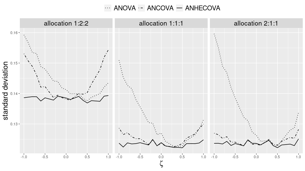
Figure 1: Standard deviations of ANOVA, ANCOVA, and ANHECOVA estimators based on 10,000 simulations and setup in (20)

Based on 10,000 simulations, all three estimators have negligible biases and their standard deviations are plotted in Figure 1 for different values of $\zeta$ between $-1$ and 1. The simulation result shows that, as predicted by our theory, ANHECOVA is generally more efficient than the other two estimators, except when $\zeta$ is nearly $0$ where ANCOVA is comparable to ANHECOVA. Furthermore, the simulation with allocation 1:2:2 (left panel in Figure 1) shows very clearly that there is no definite ordering of the variances of ANCOVA and ANOVA. Our Corollary 1 suggests that a balanced allocation does not guarantee the superiority of ANCOVA over ANOVA when there are multiple arms (in contrast with the case of two arms), which can be seen from the simulations with allocation 1:1:1 (middle panel in Figure 1).

The second simulation setting is intended to examine the performance of estimators, standard errors, and the proposed 95% asymptotic confidence intervals for $\theta_{2}-\theta_{1}$ and $\theta_{3}-\theta_{1}$, under three randomizations schemes, simple randomization, stratified permuted block, and Pocock-Simon’s minimization, with allocation 1:1:1 or 1:2:2. For each simulation, a random sample of size $n=200$ or 400 is drawn from the 481 subjects’ $(Y^{(1)},U,W)$ with replacement, and $Y^{(2)}$ and $Y^{(3)}$ are generated according to

$$\begin{split}Y^{(2)}&=-1.3+Y^{(1)}-0.5(U-\mu_{U})-0.01(U^{2}-\mu_{U^{2}})+0.3(W-\mu_{W})\\ Y^{(3)}&=-1+Y^{(1)}-0.1(U-\mu_{U})-0.01(U^{2}-\mu_{U^{2}})-0.1(W-\mu_{W})\end{split}$$ (21)

(average treatment effects $\theta_{2}-\theta_{1}=-1.3$ and $\theta_{3}-\theta_{1}=-1$). The magnitude of treatment-by-covariate interaction is represented by the differences of $\beta_{t}$-values, where for $X=(U,W)^{T}$, $\beta_{1}=(-0.240,-0.001)^{T}$, $\beta_{2}=(-0.853,0.298)^{T}$, and $\beta_{3}=(-0.453,-0.102)^{T}$. Note that a quadratic term $U^{2}-\mu_{U^{2}}$ appears in the data generating process (21) but is not adjusted by ANCOVA or ANHECOVA. Thus, the models for $Y^{(2)}-Y^{(1)}$ and $Y^{(3)}-Y^{(1)}$ are misspecified, in addition to the likely event that the model for $Y^{(1)}$ is misspecified.

The covariate $Z$ used in randomization is composed of a three-level discretized $W$ (with proportions 0.24, 0.22, and 0.54) and a two-level discretized $U$ (with proportions 0.77 and 0.23). These $Z$-categories are created according to the disease severity encoded by covariates $U$ and $W$. For stratified permuted block randomization, block size 6 is used under treatment allocation 1:1:1 and block size 10 is used under treatment allocation 1:2:2.

For ANCOVA and ANHECOVA, we consider two working models with different choices of $X$. One model includes the dummy variables for $Z$ but not $(U,W)$, motivated by the fact that $Z$ is a discretization of $(U,W)$. The other model includes not only the dummy variables for $Z$, but also $U$ and $W$. The simulation results with $n=200$ and $n=400$ based on 10,000 simulations are shown in Tables 1 and 2 respectively.

Note that in the second simulation when covariate-adaptive randomization is used, for ANOVA or ANCOVA, we employ the standard error derived under simple randomization based on Theorem 1. According to our theory, it is expected that the standard errors and the related confidence intervals based on ANOVA and ANCOVA are conservative; the simulation can show how serious the conservativeness is.

The following is a summary of simulation results in Tables 1 and 2.

1. All estimators have negligible bias compared to their standard deviation.

2. ANHECOVA has the smallest standard deviation in all scenarios of our simulation. This is consistent with our asymptotic theory.

3. There is no unambiguous ordering of the standard deviations of ANCOVA and ANOVA. In particular, ANCOVA is better in estimating $\theta_{2}-\theta_{1}$ but worse in estimating $\theta_{3}-\theta_{1}$.

4. For ANHECOVA, including additional covariates $U$ and $W$ in the working model results in a smaller standard deviation, indicating that $U$ and $W$ carry more useful information than their discretized values. Interestingly, this is not always the case for ANCOVA.

5. From Tables 1 and 2, the performances of ANHECOVA are nearly the same under three randomization schemes, the simple randomization, stratified permuted block, and Pocock-Simon’s minimization. This supports the universality results in our asymptotic theory.

6. Under simple randomization, the robust standard errors for all model-assisted estimators are very close to their actual standard deviations, and confidence intervals have nominal coverage in all settings. However, although this is still true for ANHECOVA under stratified permuted block and Pocock-Simon’s minimization, it is not the case for ANOVA and ANCOVA, i.e., standard errors valid under simple randomization appear to overestimate the actual standard deviations, so the confidence intervals are conservative. This observation reflects the universality property of ANHECOVA.

4.2 A real data example

We further illustrate the different model-assisted procedures using a real data example. Chong et al., (2016) conducted a randomized experiment to evaluate the impact of low dietary iron intake on human capital attainment. They recruited students of age 11 to 19 in a rural area of Cajamarca, Peru, where many adolescents suffer from iron deficiency. The goal of this randomized trial is to quantify the causal effect of reduced adolescent anemia on school attainment. By using students’ school grade as covariate $Z$ with five levels, a stratified permuted block randomization with 1:1:1 allocation was applied to assign 219 students to one of the following three promotional videos:

Video 1:

A popular soccer player is encouraging iron supplements to maximize energy;

Video 2:

A physician is encouraging iron supplements for overall health;

Video 3:

A dentist encouraging oral hygiene without mentioning iron at all.

Chong et al., (2016) investigated whether showing different promotional videos to the students can improve their academic performance through increased iron intake. Video 3 is treated as a “placebo”. After the treatment assignments, four students were excluded from the analysis for various reasons, which we also ignore in our analysis. The dataset is available at https://www.openicpsr.org/openicpsr/project/113624/version/V1/view.

Chong et al., (2016) used various outcomes in their analysis; here we focus on one of their primary outcomes—the academic achievement—as an example. In this trial, the academic achievement is measured by a standardized average of the student’s grades in math, foreign language, social sciences, science, and communications in a semester. For the model-assisted approaches, we use the baseline anemia status as the covariate in working models (2) and (3), which is believed to moderate the treatment effect (Chong et al.,, 2016).

Table 3 reports the analysis results by using different model-assisted procedures. Like in our simulation studies, the standard errors for ANOVA and ANCOVA are computed using estimator based on Theorem 1 for simple randomization, even though the randomization scheme here is covariate-adaptive. All the model-assisted estimators find similar effect sizes for the two contrasts (physician versus placebo, soccer star versus placebo), and the two ANHECOVA estimators have slightly smaller standard errors. Including baseline anemia status in the working model are useful to reduce the standard error. Compared to the placebo, the promotional video by the soccer player does not seem to have a positive effect on the academic achievement. In contrast, the video of the physician promoting iron supplements appears to have a positive effect. The difference between ANHECOVA and ANOVA or ANCOVA, and between including and not including anemia can be seen from the magnitude of the corresponding p-values.

5 Recommendation and Discussion

To improve its credibility and efficiency, we believe a clinical trial analysis can benefit from considerations outlined in §1.1 and discussed throughout §2-3.

Our theoretical investigation shows that the ANHECOVA with all joint levels of $Z$ included in heterogeneous working model (3), coupled with the robust variance estimator given by (19), achieves guaranteed efficiency gain over benchmark ANOVA, asymptotic optimality among a large class of estimators, wide applicability and universality. Thus, we believe it deserves wider usage in the clinical trial practice. In addition to all joint levels of $Z$, other baseline covariates highly associated with the responses can also be included in the ANHECOVA working model, following the guidance of FDA, (2021). Our theory shows that using ANOVA, ANCOVA with model (2), or ANHECOVA not adjusting for all joint levels of $Z$, suffers from invalidity, inefficiency, or non-universality in the sense that the asymptotic distribution of the estimator depends on a particular randomization scheme.

Our model-assisted asymptotic theory is given in terms of the joint asymptotic distribution in estimating $\theta$, the vector of mean responses, with multiple treatment arms under a wide range of covariate-adaptive randomization schemes. It can be readily used for inference about linear or nonlinear functions of $\theta$, with either continuous or discrete responses. Although working models (2) and (3) are not commonly used for discrete responses, ANHECOVA is still asymptotically valid as it is model-assisted. For binary responses, a popular model is logistic regression. However, if $X$ has a continuous component, the standard logistic regression inference is model-based instead of model-assisted and, thus, it may be invalid if the logistic model is not correctly specified. It should also be noted that the standard logistic regression attempts to estimate a conditional treatment effect, which is distinct from the unconditional treatment effect considered in this article due to a phenomenon called non-collapsibility; see related discussion in Gail et al., (1984), Freedman, 2008b and FDA, (2021). Recently, Wang et al., 2019b has obtained some interesting results regarding how to carry out model-assisted inference on a linear contrast of $\theta$ using logistic regression under stratified biased coin and stratified permuted block randomization.

Multiple treatment arms, which usually include a placebo, different doses (or regimens) of a new treatment, and/or active controls, are common in clinical trials (Juszczak et al.,, 2019) and are prevalent in some therapeutic areas such as immunology (Yates et al.,, 2021). In some applications, the primary analysis may focus on comparing just two treatments, even though the trial contains more than two treatment arms. A simple way of analysis is to ignore the data from other arms and apply inference procedures to the two arms of interest. For ANOVA, this is equivalent to using all the arms, since ANOVA does not borrow strength from other arms through using covariates. However, using data from all arms is recommended for ANHECOVA, because it utilizes covariate data from arms other than the two arms of interest to gain efficiency. Regarding ANCOVA, there is no definite order of efficiency for using the whole dataset or data from two given arms, since using more covariate data in ANCOVA may increase or decrease efficiency.

Our Theorem 2 can also be applied to rerandomization schemes (Li et al.,, 2018; Li and Ding,, 2020) with discrete covariates. Rerandomization attempts to balance the treatment assignments across levels of $Z$, but unlike sequential covariate-adaptive randomization, it randomizes the treatment assignments for all patients simultaneously. For two-armed trials, Corollaries 1 and 2 in Li et al., (2018) show that rerandomization satisfies (C2). Similar results for model-assisted inference can also be found in Li and Ding, (2020, Theorem 3).

As a final cautionary note, standard software does not produce asymptotically valid standard errors for model-assisted inference. We implement an R package called RobinCar to compute the model-assisted estimators and their robust standard errors, which is available at the first author’s website.

Supplementary Material

The supplementary material contains all technical proofs.

Table 1: Bias, standard deviation (SD), average standard error (SE), and coverage probability (CP) of 95% asymptotic confidence interval under simple randomization (SR), stratified permuted block randomization (PB), and Pocock-Simon’s minimization based on 10,000 simulations and setup in (21) with $n=200$

				$\theta_{2}-\theta_{1}$					$\theta_{3}-\theta_{1}$
Allocation	Randomization	Method	$X$	Bias	SD	SE	CP		Bias	SD	SE	CP
1:1:1	SR	ANOVA		-0.002	0.467	0.463	0.944		0.000	0.284	0.285	0.950
		ANCOVA	$Z$	0.000	0.445	0.433	0.941		-0.001	0.326	0.322	0.949
		ANCOVA	$Z,U,W$	-0.023	0.428	0.407	0.933		0.009	0.351	0.339	0.942
		ANHECOVA	$Z$	0.000	0.384	0.372	0.939		0.003	0.238	0.235	0.943
		ANHECOVA	$Z,U,W$	0.000	0.325	0.315	0.943		0.001	0.220	0.213	0.941
	PB	ANOVA		-0.002	0.380	0.462	0.980		-0.001	0.241	0.284	0.977
		ANCOVA	$Z$	-0.002	0.379	0.432	0.972		-0.001	0.242	0.321	0.991
		ANCOVA	$Z,U,W$	-0.026	0.356	0.406	0.970		0.009	0.275	0.338	0.983
		ANHECOVA	$Z$	-0.002	0.377	0.371	0.940		-0.001	0.240	0.234	0.940
		ANHECOVA	$Z,U,W$	-0.002	0.317	0.314	0.948		-0.001	0.220	0.213	0.941
	Minimization	ANOVA		0.003	0.378	0.463	0.980		0.002	0.236	0.284	0.981
		ANCOVA	$Z$	0.003	0.378	0.432	0.972		0.002	0.237	0.321	0.991
		ANCOVA	$Z,U,W$	-0.021	0.356	0.406	0.968		0.012	0.270	0.338	0.985
		ANHECOVA	$Z$	0.002	0.376	0.372	0.946		0.002	0.236	0.234	0.947
		ANHECOVA	$Z,U,W$	0.002	0.319	0.314	0.945		0.003	0.217	0.213	0.943
1:2:2	SR	ANOVA		0.001	0.446	0.441	0.946		0.003	0.289	0.289	0.949
		ANCOVA	$Z$	0.004	0.430	0.417	0.942		0.002	0.347	0.339	0.946
		ANCOVA	$Z,U,W$	-0.019	0.420	0.398	0.934		0.012	0.380	0.365	0.943
		ANHECOVA	$Z$	0.003	0.386	0.382	0.945		0.004	0.257	0.256	0.947
		ANHECOVA	$Z,U,W$	0.004	0.345	0.342	0.949		0.006	0.247	0.241	0.942
	PB	ANOVA		0.002	0.379	0.441	0.977		0.000	0.254	0.289	0.971
		ANCOVA	$Z$	0.002	0.378	0.414	0.968		0.000	0.257	0.337	0.988
		ANCOVA	$Z,U,W$	-0.024	0.365	0.395	0.961		0.008	0.296	0.362	0.982
		ANHECOVA	$Z$	0.001	0.377	0.381	0.951		0.000	0.253	0.255	0.948
		ANHECOVA	$Z,U,W$	0.002	0.336	0.341	0.948		0.001	0.243	0.240	0.944
	Minimization	ANOVA		0.003	0.384	0.441	0.971		0.000	0.251	0.288	0.974
		ANCOVA	$Z$	0.001	0.383	0.414	0.961		-0.002	0.252	0.336	0.991
		ANCOVA	$Z,U,W$	-0.023	0.371	0.395	0.959		0.008	0.294	0.361	0.985
		ANHECOVA	$Z$	0.002	0.382	0.381	0.944		-0.001	0.250	0.254	0.950
		ANHECOVA	$Z,U,W$	0.000	0.338	0.341	0.952		-0.001	0.239	0.239	0.948

Table 2: Bias, standard deviation (SD), average standard error (SE), and coverage probability (CP) of 95% asymptotic confidence interval under simple randomization (SR), stratified permuted block randomization (PB), and Pocock-Simon’s minimization based on 10,000 simulations and setup in (21) with $n=400$

				$\theta_{2}-\theta_{1}$					$\theta_{3}-\theta_{1}$
Allocation	Randomization	Method	$X$	Bias	SD	SE	CP		Bias	SD	SE	CP
1:1:1	SR	ANOVA		0.001	0.327	0.327	0.946		-0.001	0.201	0.201	0.949
		ANCOVA	$Z$	0.001	0.310	0.306	0.945		0.000	0.229	0.227	0.949
		ANCOVA	$Z,U,W$	-0.011	0.295	0.289	0.944		0.003	0.246	0.240	0.945
		ANHECOVA	$Z$	-0.001	0.271	0.265	0.944		-0.002	0.169	0.167	0.949
		ANHECOVA	$Z,U,W$	0.000	0.226	0.224	0.947		-0.002	0.155	0.152	0.948
	PB	ANOVA		0.000	0.267	0.327	0.982		-0.001	0.166	0.201	0.982
		ANCOVA	$Z$	0.001	0.267	0.306	0.975		-0.001	0.166	0.227	0.992
		ANCOVA	$Z,U,W$	-0.012	0.250	0.289	0.974		0.003	0.186	0.240	0.987
		ANHECOVA	$Z$	0.001	0.266	0.265	0.947		-0.001	0.165	0.167	0.950
		ANHECOVA	$Z,U,W$	0.002	0.224	0.224	0.950		-0.001	0.152	0.152	0.948
	Minimization	ANOVA		-0.002	0.268	0.327	0.982		0.000	0.168	0.201	0.980
		ANCOVA	$Z$	-0.002	0.267	0.306	0.974		0.000	0.168	0.227	0.992
		ANCOVA	$Z,U,W$	-0.013	0.250	0.289	0.974		0.005	0.189	0.240	0.987
		ANHECOVA	$Z$	-0.002	0.267	0.265	0.948		0.000	0.167	0.167	0.949
		ANHECOVA	$Z,U,W$	-0.001	0.225	0.223	0.946		0.000	0.154	0.152	0.944
1:2:2	SR	ANOVA		0.001	0.311	0.312	0.951		0.000	0.205	0.204	0.951
		ANCOVA	$Z$	0.001	0.298	0.294	0.947		0.001	0.241	0.239	0.950
		ANCOVA	$Z,U,W$	-0.013	0.286	0.281	0.945		0.003	0.262	0.257	0.947
		ANHECOVA	$Z$	0.000	0.268	0.268	0.949		0.001	0.182	0.180	0.948
		ANHECOVA	$Z,U,W$	0.001	0.237	0.238	0.949		0.002	0.171	0.169	0.944
	PB	ANOVA		0.002	0.265	0.312	0.977		0.001	0.180	0.204	0.975
		ANCOVA	$Z$	0.002	0.265	0.293	0.969		0.001	0.181	0.238	0.991
		ANCOVA	$Z,U,W$	-0.012	0.253	0.280	0.967		0.005	0.207	0.256	0.986
		ANHECOVA	$Z$	0.002	0.264	0.267	0.950		0.001	0.179	0.179	0.949
		ANHECOVA	$Z,U,W$	0.001	0.234	0.238	0.951		0.002	0.170	0.168	0.946
	Minimization	ANOVA		0.000	0.265	0.311	0.979		0.002	0.181	0.204	0.971
		ANCOVA	$Z$	-0.001	0.265	0.293	0.969		0.001	0.182	0.238	0.991
		ANCOVA	$Z,U,W$	-0.013	0.253	0.280	0.970		0.006	0.208	0.256	0.985
		ANHECOVA	$Z$	-0.001	0.265	0.267	0.951		0.001	0.181	0.179	0.947
		ANHECOVA	$Z,U,W$	0.001	0.233	0.238	0.956		0.002	0.172	0.168	0.945

Table 3: Estimate, standard error (SE), and p-value in the real data example analysis

			Physician versus placebo				Soccer star versus placebo
Method	$X$		Estimate	SE	p-value		Estimate	SE	p-value
ANOVA			0.386	0.211	0.067		-0.068	0.205	0.739
ANCOVA	Grade		0.403	0.203	0.046		-0.052	0.203	0.799
	Grade, Anemia status		0.437	0.199	0.028		-0.085	0.201	0.672
ANHECOVA	Grade		0.409	0.200	0.041		-0.051	0.201	0.800
	Grade, Anemia status		0.481	0.193	0.013		-0.046	0.195	0.815

1 Two Lemmas

Lemma 2.

Assume (C1), (C2), and that $P(A_{i}=a_{t}\mid Z_{1},\dots,Z_{n})=\pi_{t}$ for all $t=1,\dots,k$ and $i=1,\dots,n$. We have the following conclusions.
(i) For any integrable function $f$,

$$E\{f(Y_{i}^{(t)},X_{i})\}=E(f(Y_{i},X_{i})\mid A_{i}=a_{t})$$

and

$$E\{f(Y_{i}^{(t)},X_{i})\mid X_{i}\}=E(f(Y_{i},X_{i})\mid X_{i},A_{i}=a_{t}).$$

(ii) Let $\theta=(E(Y^{(1)},...,E(Y^{(k)}))^{\top}$ be the potential response mean vector, ${\beta}=\sum_{t=1}^{k}\pi_{t}\beta_{t}$, and $\beta_{t}=\Sigma_{X}^{-1}{\rm cov}(X_{i},Y_{i}^{(t)})$, $t=1,...,k$. Then

$$(\theta,{\beta})=\arg\min_{(\vartheta,\beta\!\!\!/)}E\left[\left\{Y_{i}-\vartheta^{\top}A_{i}-\beta\!\!\!/^{\top}(X_{i}-\mu_{X})\right\}^{2}\right]$$

and

$$(\theta,\beta_{1},\dotsc,\beta_{k})=\arg\min_{(\vartheta,\beta\!\!\!/_{1},\dotsc,\beta\!\!\!/_{k})}E\left[\left\{Y_{i}-\vartheta^{\top}A_{i}-\sum_{t=1}^{k}\beta\!\!\!/_{t}^{\top}(X_{i}-\mu_{X})I(A_{i}=a_{t})\right\}^{2}\right].$$

The condition $P(A_{i}=a_{t}\mid Z_{1},\dots,Z_{n})=\pi_{t}$ for all $t$ and $i$ holds for most covariate-adaptive randomization schemes. Note that it does not exclude the possibility that the set of random variables $\{A_{i},i=1,\dotsc,n\}$ is dependent of $\{Z_{i},i=1,\dotsc,n\}$, which is indeed the case for covariate-adaptive randomization schemes. We impose this condition only in Lemma 2 to facilitate understanding the working models. This additional assumption is not needed for our asymptotic theory in §3, as condition (C2) is sufficient.

Proof.

(i) We focus on proving the second result; the first result can be shown similarly. For simple randomization, this result immediately follows (C2) (i) as $(Y_{i}^{(1)},\dotsc,Y_{i}^{(k)},X_{i},A_{i})$ are independent and identically distributed. For covariate-adaptive randomization, we remark that the property of conditional independence (Dawid,, 1979, Lemma 4.3), (C2) (i) and the third condition in Lemma 2 imply that $A_{i}$ is independent of $\{(Y_{i}^{(1)},...,Y_{i}^{(k)},X_{i},Z_{i}),i=1,\dotsc,n\}$. Then, it can be shown that

$$E\{f(Y_{i},X_{i})\mid X_{i},A_{i}=a_{t}\}= \ E\{f(Y_{i}^{(t)},X_{i})\mid X_{i},A_{i}=a_{t}\}$$

$$= \sum_{z_{1},\dotsc,z_{n}\in\mathcal{Z}}E\{f(Y_{i}^{(t)},X_{i})\mid X_{i},A_{i}=a_{t},G_{n}\}P(G_{n}\mid X_{i},A_{i}=a_{t})$$

$$= \sum_{z_{1},\dotsc,z_{n}\in\mathcal{Z}}E\{f(Y_{i}^{(t)},X_{i})\mid X_{i},G_{n}\}P(G_{n}\mid X_{i},A_{i}=a_{t})$$

$$= \sum_{z_{1},\dotsc,z_{n}\in\mathcal{Z}}E\{f(Y_{i}^{(t)},X_{i})\mid X_{i},G_{n}\}P(G_{n}\mid X_{i})$$

$$= \ E\{f(Y_{i}^{(t)},X_{i})\mid X_{i}\},$$

where $G_{n}$ is the event that $\{Z_{i}=z_{i},i=1,...,n\}$, and the equalities follow from the consistency of potential responses, the law of iterated expectation, (C2) (i), and the remark above.
(ii) We only prove the first result. The second result can be proved similarly. Let $(\theta,\beta)$ be the optimality points satisfying the following estimation equations:

$$E\big{[}I(A_{i}=a_{t})\{Y_{i}-\theta^{\top}A_{i}-\beta^{\top}(X_{i}-\mu_{X})\}\big{]}=0,\qquad\text{for any }t$$ (S1)

$$E\big{[}(X_{i}-\mu_{X})\{Y_{i}-\theta^{\top}A_{i}-\beta^{\top}(X_{i}-\mu_{X})\}\big{]}=0.$$ (S2)

From Lemma 2(i), (1) implies that for any $t$,

$$E\big{[}Y_{i}-\theta^{\top}A_{i}-\beta^{\top}(X_{i}-\mu_{X})\mid A_{i}=a_{t}\big{]}=E\big{[}Y_{i}^{(t)}-\theta_{t}-\beta^{\top}(X_{i}-\mu_{X})\big{]}=E[Y_{i}^{(t)}-\theta_{t}]=0$$

and, thus, $\theta_{t}=E(Y_{i}^{(t)})$, $t=1,...,k$. Then (S2) implies that

$$0= E\big{[}(X_{i}-\mu_{X})\{Y_{i}-\theta^{\top}A_{i}-\beta^{\top}(X_{i}-\mu_{X})\}\big{]}$$

$$= \sum_{t=1}^{k}E\big{[}I(A_{i}=a_{t})(X_{i}-\mu_{X})\{Y_{i}-\theta^{\top}A_{i}-\beta^{\top}(X_{i}-\mu_{X})\}\big{]}$$

$$= \sum_{t=1}^{k}E\big{[}(X_{i}-\mu_{X})\{Y_{i}-\theta^{\top}A_{i}-\beta^{\top}(X_{i}-\mu_{X})\}\mid A_{i}=a_{t}\big{]}\pi_{t}$$

$$= \sum_{t=1}^{k}E\big{[}(X_{i}-\mu_{X})\{Y^{(t)}_{i}-\theta_{t}-\beta^{\top}(X_{i}-\mu_{X})\}\big{]}\pi_{t}$$

$$= \sum_{t=1}^{k}\left[{\rm cov}(X_{i},Y_{i}^{(t)})-\Sigma_{X}\beta\right]\pi_{t}$$

$$= \sum_{t=1}^{k}{\rm cov}(X_{i},Y_{i}^{(t)})\pi_{t}-\Sigma_{X}\beta$$

and, thus, $\beta=\Sigma_{X}^{-1}\sum_{t=1}^{k}{\rm cov}(X_{i},Y_{i}^{(t)})\pi_{t}=\sum_{t=1}^{k}\pi_{t}\beta_{t}$. ∎

Lemma 3.

Under conditions (C1)-(C2), for $t=1,\dots,k$, $\hat{\beta}_{t}=\beta_{t}+o_{p}(1)$ and $\hat{\beta}=\beta+o_{p}(1)$;

Proof.

(i) We prove the result for $\hat{\beta}_{t}$. The proof for $\hat{\beta}$ is analogous and omitted. Notice that

$$\frac{1}{n_{t}}\sum_{i:A_{i}=a_{t}}(X_{i}-\bar{X}_{t})Y_{i}=\frac{1}{n_{t}}\sum_{i=1}^{n}I(A_{i}=a_{t})X_{i}Y_{i}-\frac{1}{n_{t}}\sum_{i=1}^{n}I(A_{i}=a_{t})X_{i}\frac{1}{n_{t}}\sum_{i=1}^{n}I(A_{i}=a_{t})Y_{i}$$

Let $\mathcal{A}=\{A_{1},\dots,A_{n}\}$ and $\mathcal{F}=\{Z_{1},\dots,Z_{n}\}$. Note that

$$E\left\{\frac{1}{n}\sum_{i=1}^{n}I(A_{i}=a_{t})X_{i}Y_{i}\mid\mathcal{A},\mathcal{F}\right\} =\frac{1}{n}\sum_{i=1}^{n}I(A_{i}=a_{t})E(X_{i}Y_{i}^{(t)}\mid\mathcal{A},\mathcal{F})$$

$$=\frac{1}{n}\sum_{i=1}^{n}I(A_{i}=a_{t})E(X_{i}Y_{i}^{(t)}\mid Z_{i}),$$

where the second line holds because $E(X_{i}Y_{i}^{(t)}\mid\mathcal{A},\mathcal{F})=E(X_{i}Y_{i}^{(t)}\mid\mathcal{F})=E(X_{i}Y_{i}^{(t)}\mid Z_{i})$ from (C1) and (C2) (i). Moreover, $n^{-1}\sum_{i=1}^{n}I(A_{i}=a_{t})X_{i}Y_{i}^{(t)}$ is an average of independent random variables once conditional on $\{\mathcal{A},\mathcal{F}\}$. From the existence of second moment of $XY^{(t)}$, and the weak law of large numbers for independent random variables, we conclude that, for any $\epsilon>0$,

$$\lim_{n\rightarrow\infty}P\left(\bigg{|}\frac{1}{n}\sum_{i=1}^{n}I(A_{i}=a_{t})X_{i}Y_{i}-\frac{1}{n}\sum_{i=1}^{n}I(A_{i}=a_{t})E(X_{i}Y_{i}^{(t)}\mid Z_{i})\bigg{|}\geq\epsilon\,\mid\,\mathcal{A},\mathcal{F}\right)=0$$

From the bounded convergence theorem, the above equation also holds unconditionally. In other words,

$$\frac{1}{n}\sum_{i=1}^{n}I(A_{i}=a_{t})X_{i}Y_{i}-\frac{1}{n}\sum_{i=1}^{n}I(A_{i}=a_{t})E(X_{i}Y_{i}^{(t)}\mid Z_{i})=o_{p}(1).$$

Furthermore,

$$\frac{1}{n}\sum_{i=1}^{n}I(A_{i}=a_{t})E(X_{i}Y_{i}^{(t)}\mid Z_{i}) =\frac{1}{n}\sum_{z}\sum_{i=1}^{n}I(Z_{i}=z)I(A_{i}=a_{t})E(X_{i}Y_{i}^{(t)}\mid Z_{i}=z)$$

$$=\frac{1}{n}\sum_{z}E(X_{i}Y_{i}^{(t)}\mid Z_{i}=z)\sum_{i=1}^{n}I(Z_{i}=z)I(A_{i}=a_{t})$$

$$=\frac{1}{n}\sum_{z}E(X_{i}Y_{i}^{(t)}\mid Z_{i}=z)n_{t}(z)$$

$$=\sum_{z}E(X_{i}Y_{i}^{(t)}\mid Z_{i}=z)\frac{n_{t}(z)}{n(z)}\frac{n(z)}{n}$$

$$=\sum_{z}E(X_{i}Y_{i}^{(t)}\mid Z_{i}=z)\pi_{t}P(Z_{i}=z)+o_{p}(1)$$

$$=\pi_{t}E(X_{i}Y_{i}^{(t)})+o_{p}(1)$$

This together with the fact that $n_{t}/n=\sum_{z}n_{t}(z)/\{\sum_{z}n(z)\}=\pi_{t}+o_{p}(1)$, we have

$$\frac{1}{n_{t}}\sum_{i=1}^{n}I(A_{i}=a_{t})X_{i}Y_{i}=E(X_{i}Y_{i}^{(t)})+o_{p}(1)$$

Similarly, we can show the result with $X_{i}Y_{i}$ replaced by $X_{i}$ or $Y_{i}$ also holds, i.e.,

$$\frac{1}{n_{t}}\sum_{i=1}^{n}I(A_{i}=a_{t})X_{i}=E(X_{i})+o_{p}(1)$$

$$\frac{1}{n_{t}}\sum_{i=1}^{n}I(A_{i}=a_{t})Y_{i}=E(Y_{i}^{(t)})+o_{p}(1)$$

The denominator of $\hat{\beta}_{t}$ can be treated similarly, which leads to

$$\frac{1}{n_{t}}\sum_{i:A_{i}=a_{t}}\{X_{i}-\bar{X}_{t}\}\{X_{i}-\bar{X}_{t}\}^{\top}=\Sigma_{X}+o_{p}(1).$$

The proof is completed by using the definition of $\beta_{t}$.

∎

2 Technical Proofs

2.1 Proof of (9)

Under simple randomization, $A_{1},\dots,A_{n}$ are independent with other variables. Let $\bar{X}_{-t}=(n-n_{t})^{-1}\sum_{i:A_{i}\neq a_{t}}X_{i}$. Then $\bar{X}_{t}-\bar{X}=n^{-1}(n-n_{t})(\bar{X}_{t}-\bar{X}_{-t})$. Note that $\bar{X}_{t}$ and $\bar{X}_{-t}$ are uncorrelated conditional on $\mathcal{A}=(A_{1},...,A_{n})$, as

$${\rm cov}(\bar{X}_{t},\bar{X}_{-t}\mid\mathcal{A})=\frac{1}{(n-n_{t})n_{t}}\sum_{i=1}^{n}\sum_{j=1}^{n}I(A_{i}=a_{t})I(A_{j}\neq a_{t}){\rm cov}(X_{i},X_{j}\mid\mathcal{A})=0,$$

where the last equality is from ${\rm cov}(X_{i},X_{j}\mid\mathcal{A})={\rm cov}(X_{i},X_{j})=0$ for $i\neq j$. Similarly, we can show that $\bar{Y}_{t}$ and $\bar{X}_{-t}$ are uncorrelated conditional on $\mathcal{A}$.

Then,

$${\rm cov}\{\beta_{t}^{\top}(\bar{X}_{t}-\bar{X}),\bar{Y}_{t}\} =\beta_{t}^{\top}{\rm cov}\left(\frac{n-n_{t}}{n}\bar{X}_{t}-\frac{n-n_{t}}{n}\bar{X}_{-t},\bar{Y}_{t}\right)$$

$$=\beta_{t}^{\top}E\left\{{\rm cov}\left(\frac{n-n_{t}}{n}\bar{X}_{t},\bar{Y}_{t}\mid{\cal A}\right)\right\}$$

$$=\beta_{t}^{\top}E\left\{\frac{n-n_{t}}{nn_{t}^{2}}{\rm cov}\left(\sum_{i:A_{i}=a_{t}}X_{i},\sum_{i:A_{i}=a_{t}}Y_{i}\mid\mathcal{A}\right)\right\}$$

$$=\beta_{t}^{\top}E\left\{\frac{n-n_{t}}{nn_{t}^{2}}\sum_{i:A_{i}=a_{t}}{\rm cov}\left(X_{i},Y_{i}^{(t)}\right)\right\}$$

$$=\beta_{t}^{\top}E\left\{\frac{n-n_{t}}{nn_{t}}\right\}{\rm cov}\left(X_{i},Y_{i}^{(t)}\right)$$

$$=E\left\{\frac{n-n_{t}}{nn_{t}}\right\}\beta_{t}^{\top}\Sigma_{X}\beta_{t}$$

where the second equality is from ${\rm cov}(\bar{X}_{-t},\bar{Y}_{t}\mid\mathcal{A})=0$, $E(\bar{Y}_{t}\mid\mathcal{A})=E(Y^{(t)})$ and the identity that ${\rm cov}(X,Y)=E\{{\rm cov}(X,Y\mid Z)\}+{\rm cov}\{E(X\mid Z),E(Y\mid Z)\}$. Also note that

$${\rm var}\{\beta_{t}^{\top}(\bar{X}_{t}-\bar{X})\} =\beta_{t}^{\top}{\rm var}\left(\frac{n-n_{t}}{n}(\bar{X}_{t}-\bar{X}_{-t})\right)\beta_{t}$$

$$=\beta_{t}^{\top}E\left(\frac{(n-n_{t})^{2}}{n^{2}}{\rm var}(\bar{X}_{t}-\bar{X}_{-t}\mid\mathcal{A})\right)\beta_{t}$$

$$=\beta_{t}^{\top}E\left(\frac{(n-n_{t})^{2}}{n^{2}}\{{\rm var}(\bar{X}_{t}\mid\mathcal{A})+{\rm var}(\bar{X}_{-t}\mid\mathcal{A})\}\right)\beta_{t}$$

$$=\beta_{t}^{\top}E\left(\frac{(n-n_{t})^{2}}{n^{2}}\left\{\frac{{{\rm var}(X_{i})}}{n_{t}}+\frac{{{\rm var}(X_{i})}}{n-n_{t}}\right\}\right)\beta_{t}$$

$$=E\left\{\frac{n-n_{t}}{nn_{t}}\right\}\beta_{t}^{\top}\Sigma_{X}\beta_{t}$$

where the second equality uses the identity that ${\rm var}(X)=E\{{\rm var}(X\mid Z)\}+{\rm var}\{E(X\mid Z)\}$, and $E\left(\bar{X}_{t}-\bar{X}_{-t}\mid\mathcal{A}\right)=E(X_{i})-E(X_{i})=0$.

2.2 Proof of Lemma 1

For any fixed $k$-dimensional vector $\ell=(\ell_{1},\dots,\ell_{k})^{\top}$, we have

$$\ell^{\top}\{{\rm diag}(\pi_{t}^{-1}m_{t}^{\top}m_{t})-M^{\top}M\}\ell$$

$$= \sum_{t=1}^{k}\pi_{t}^{-1}\ell_{t}^{2}m_{t}^{\top}m_{t}-\left\{\sum_{t=1}^{k}\ell_{t}m_{t}^{\top}\right\}\left\{\sum_{t=1}^{k}\ell_{t}m_{t}\right\}$$

$$= E(Q^{\top}Q)-E(Q^{\top})E(Q)$$

$$= \text{tr}\{E(QQ^{\top})\}-\text{tr}\{E(Q)E(Q^{\top})\}$$

$$\geq 0,$$

where ${\rm tr}$ denotes the trace of a matrix, $Q$ denotes a $p$-dimensional random vector that takes value $\pi_{t}^{-1}\ell_{t}m_{t}$ with probability $\pi_{t}$, $t=1,\dots,k$, and the last equality follows from the fact that the covariance matrix $\text{var}(Q)=E(QQ^{\top})-E(Q)E(Q^{\top})$ is positive semidefinite.

2.3 Proof of Theorem 1

(i) First, from $\bar{X}_{t}-\bar{X}=O_{p}(n^{-1/2})$ and $\hat{b}_{t}=b_{t}+o_{p}(1)$, we have

$$\hat{\theta}(\hat{b}_{1},\dots,\hat{b}_{k}) = \hat{\theta}(b_{1},\dots,b_{k})+\{(\bar{X}_{1}-\bar{X})(b_{1}-\hat{b}_{1}),\dots,(\bar{X}_{1}-\bar{X})(b_{k}-\hat{b}_{k})\}^{\top}$$

$$= \hat{\theta}(b_{1},\dots,b_{k})+o_{p}(n^{-1/2}).$$

Write the sample average as $\mathbb{E}_{n}[\mu(X)]=n^{-1}\sum_{i=1}^{n}\mu(X_{i})$. Then,

$$\bar{X}-\mu_{X} =\sum_{t=1}^{k}\frac{1}{n}\sum_{i=1}^{n}I(A_{i}=a_{t})(X_{i}-\mu_{X})=\sum_{t=1}^{k}\mathbb{E}_{n}\left[I(A=a_{t})(X-\mu_{X})\right],$$

and

$$\bar{Y}_{t}-\theta_{t}-(\bar{X}_{t}-\mu_{X})^{\top}b_{t}$$

$$=\frac{1}{n_{t}}\sum_{i=1}^{n}I(A_{i}=a_{t})\left\{Y_{i}-\theta_{t}-(X_{i}-\mu_{X})^{\top}b_{t}\right\}$$

$$=\pi_{t}^{-1}\frac{1}{n}\sum_{i=1}^{n}I(A_{i}=a_{t})\left\{Y_{i}-\theta_{t}-(X_{i}-\mu_{X})^{\top}b_{t}\right\}$$

$$\qquad+\left(\frac{1}{n_{t}/n}-\frac{1}{\pi_{t}}\right)\frac{1}{n}\sum_{i=1}^{n}I(A_{i}=a_{t})\left\{Y_{i}-\theta_{t}-(X_{i}-\mu_{X})^{\top}b_{t}\right\}$$

$$=\pi_{t}^{-1}\mathbb{E}_{n}\left[I(A=a_{t})\{Y-\theta_{t}-(X-\mu_{X})^{\top}b_{t}\}\right]+o_{p}(n^{-1/2}),$$

where the last equality holds because $\mathbb{E}_{n}\left[I(A=a_{t})\{Y-\theta_{t}-(X-\mu_{X})^{\top}b_{t}\}\right]=O_{p}(n^{-1/2})$ from the central limit theorem, and $n/n_{t}-\pi_{t}^{-1}=o_{p}(1)$ from condition (C2) (ii). Hence, we can decompose $\hat{\theta}(b_{1},\dots,b_{k})$ as

$$\hat{\theta}(b_{1},\dots,b_{k})-\theta$$

$$=\left(\begin{array}[]{c}\bar{Y}_{1}-\theta_{1}-(\bar{X}_{1}-\mu_{X})^{\top}b_{1}\\ \vdots\\ \bar{Y}_{k}-\theta_{k}-(\bar{X}_{k}-\mu_{X})^{\top}b_{k}\end{array}\right)+\left(\begin{array}[]{c}b_{1}^{\top}(\bar{X}-\mu_{X})\\ \vdots\\ b_{k}^{\top}(\bar{X}-\mu_{X})\end{array}\right)$$

$$=\underbrace{\left(\begin{array}[]{c}\pi_{1}^{-1}\mathbb{E}_{n}\left[I(A=a_{1})\{Y-\theta_{1}-(X-\mu_{X})^{\top}b_{1}\}\right]\\ \vdots\\ \pi_{k}^{-1}\mathbb{E}_{n}\left[I(A=a_{k})\{Y-\theta_{k}-(X-\mu_{X})^{\top}b_{k}\}\right]\end{array}\right)}_{M_{1}}+\underbrace{\left(\begin{array}[]{c}b_{1}^{\top}\sum_{t=1}^{k}\mathbb{E}_{n}\left[I(A=a_{t})(X-\mu_{X})\right]\\ \vdots\\ b_{k}^{\top}\sum_{t=1}^{k}\mathbb{E}_{n}\left[I(A=a_{t})(X-\mu_{X})\right]\end{array}\right)}_{M_{2}}$$

$$\qquad+o_{p}(n^{-1/2})$$

$$=\left(\begin{array}[]{ccccc}\pi_{1}^{-1}a_{1}^{\top}&-\pi_{1}^{-1}b_{1}^{\top}&{0}_{p}^{\top}&\cdots&{0}_{p}^{\top}\\ \vdots&\vdots&\vdots&\ddots&\vdots\\ \pi_{k}^{-1}a_{k}^{\top}&{0}_{p}^{\top}&{0}_{p}^{\top}&\cdots&-\pi_{k}^{-1}b_{k}^{\top}\end{array}\right)_{k\times(k+kp)}\underbrace{\left(\begin{array}[]{c}\mathbb{E}_{n}\left[I(A=a_{1})(Y-\theta_{1})\right]\\ \vdots\\ \mathbb{E}_{n}\left[I(A=a_{k})(Y-\theta_{k})\right]\\ \mathbb{E}_{n}\left[I(A=a_{1})(X-\mu_{X})\right]\\ \vdots\\ \mathbb{E}_{n}\left[I(A=a_{k})(X-\mu_{X})\right]\end{array}\right)}_{V_{(k+kp)\times 1}}$$

$$+\left(\begin{array}[]{ccccc}b_{1}^{\top}&b_{1}^{\top}&\dots&b_{1}^{\top}\\ \vdots&\vdots&\ddots&\vdots\\ b_{k}^{\top}&b_{k}^{\top}&\dots&b_{k}^{\top}\end{array}\right)_{k\times(kp)}\left(\begin{array}[]{c}\mathbb{E}_{n}\left[I(A=a_{1})(X-\mu_{X})\right]\\ \vdots\\ \mathbb{E}_{n}\left[I(A=a_{k})(X-\mu_{X})\right]\end{array}\right)_{(k+kp)\times 1}+o_{p}(n^{-1/2}),$$

where $a_{t}$ denotes the $k$-dimensional vector whose $t$th component is 1 and other components are 0, $p$ is the dimension of $X$, $0_{p}$ denotes a $p$-dimensional vector of zeros. From the central limit theorem, we have that the random vector $\sqrt{n}V$ is asymptotically normal with mean 0. This implies that $\sqrt{n}\{\hat{\theta}(b_{1},\dots,b_{k})-\theta\}$ is asymptotically normal with mean 0 from the Cramér-Wold device.

It remains to calculate the asymptotic variance of $\sqrt{n}\{\hat{\theta}(b_{1},\dots,b_{k})-\theta\}$. In the following, we consider $M_{1}$ and $M_{2}$ separately.

Consider $M_{1}$, where the $t$th component equals

$$M_{1t}=\pi_{t}^{-1}\mathbb{E}_{n}\left[I(A=a_{t})\{Y-\theta_{t}-(X-\mu_{X})^{\top}b_{t}\}\right].$$

We have that $(M_{1t},t=1,\dots,k)$ are mutually independent and

$${\rm var}(M_{1t})=(n\pi_{t})^{-1}{\rm var}\{Y^{(t)}-X^{\top}b_{t}\},$$

Hence, ${\rm var}(M_{1})$ is a diagonal matrix, with the diagonal elements being ${\rm var}(M_{1t}),t=1,\dots,k$. That is, $n{\rm var}(M_{1})={\rm diag}\{\pi_{t}^{-1}{\rm var}(Y^{(t)}-X^{\top}b_{t})\}$.

Next, consider $M_{2}$, which can be reformulated as

$$M_{2}=\left(\begin{array}[]{ccc}b_{1}^{\top}&&\\ &\ddots&\\ &&b_{k}^{\top}\end{array}\right)_{k\times(kp)}\left(\begin{array}[]{c}\sum_{t=1}^{k}\mathbb{E}_{n}\left[I(A=a_{t})(X-\mu_{X})\right]\\ \cdots\\ \sum_{t=1}^{k}\mathbb{E}_{n}\left[I(A=a_{t})(X-\mu_{X})\right]\end{array}\right)_{(kp)\times 1}$$

whose variance can be easily derived as $n{\rm var}(M_{2})=B^{\top}\Sigma_{X}B$.

Finally, consider ${\rm cov}(M_{1},M_{2})$ whose $(t,s)$ element equals

$${\rm cov}\left\{\pi_{t}^{-1}\mathbb{E}_{n}\left[I(A=a_{t})\{Y-\theta_{t}-(X-\mu_{X})^{\top}b_{t}\}\right],b_{s}^{\top}\sum_{t=1}^{k}\mathbb{E}_{n}\left[I(A=a_{t})(X-\mu_{X})\right]\right\}$$

$$={\rm cov}\left\{\pi_{t}^{-1}\mathbb{E}_{n}\left[I(A=a_{t})\{Y-\theta_{t}-(X-\mu_{X})^{\top}b_{t}\}\right],b_{s}^{\top}\mathbb{E}_{n}\left[I(A=a_{t})(X-\mu_{X})\right]\right\}$$

$$=n^{-1}\pi_{t}^{-1}{\rm cov}\left\{I(A=a_{t})(Y-X^{\top}b_{t})\},b_{s}^{\top}I(A=a_{t})(X-\mu_{X})\right\}$$

$$=n^{-1}\pi_{t}^{-1}E\left\{I(A=a_{t})(Y-X^{\top}b_{t})b_{s}^{\top}(X-\mu_{X})\right\}$$

$$=n^{-1}E\left\{(Y^{(t)}-X^{\top}b_{t})b_{s}^{\top}(X-\mu_{X})\right\}$$

$$=n^{-1}\left\{{\rm cov}(Y^{(t)},b_{s}^{\top}X)-{\rm cov}(X^{\top}b_{t},b_{s}^{\top}X)\right\}$$

$$=n^{-1}\{\beta_{t}^{\top}\Sigma_{X}b_{s}-b_{t}^{\top}\Sigma_{X}b_{s}\}$$

$$=n^{-1}(\beta_{t}-b_{t})^{\top}\Sigma_{X}b_{s}.$$

Thus, $n{\rm cov}(M_{1},M_{2})=(\mathscr{B}-B)^{\top}\Sigma_{X}B$ and $n{\rm cov}(M_{2},M_{1})=B^{\top}\Sigma_{X}(\mathscr{B}-B)$. Combining the above results, we conclude that $\sqrt{n}\{\hat{\theta}(b_{1},\dots,b_{k})-\theta\}$ is asymptotically normal with mean 0 and variance $V_{\rm SR}(B)$,

$$V_{\rm SR}(B) ={\rm diag}\{\pi_{t}^{-1}{\rm var}(Y^{(t)}-X^{\top}b_{t})\}+(\mathscr{B}-B)^{\top}\Sigma_{X}B+B^{\top}\Sigma_{X}(\mathscr{B}-B)+B^{\top}\Sigma_{X}B$$

$$={\rm diag}\{\pi_{t}^{-1}{\rm var}(Y^{(t)}-X^{\top}b_{t})\}+\mathscr{B}^{\top}\Sigma_{X}B+B^{\top}\Sigma_{X}\mathscr{B}-B^{\top}\Sigma_{X}B.$$

(ii) Note that

$${\rm var}(Y^{(t)}-b_{t}^{\top}X)= {\rm var}(Y^{(t)}-\beta_{t}^{\top}X+\beta_{t}^{\top}X-b_{t}^{\top}X)$$

$$= {\rm var}\{Y^{(t)}-\beta_{t}^{\top}X\}+{\rm var}\{(\beta_{t}-b_{t})^{\top}X\}+2{\rm cov}\{Y^{(t)}-\beta_{t}^{\top}X,(\beta_{t}-b_{t})^{\top}X\}$$

$$= {\rm var}\{Y^{(t)}-\beta_{t}^{\top}X\}+(\beta_{t}-b_{t})^{\top}\Sigma_{X}(\beta_{t}-b_{t}).$$

Then simple algebra shows that

$$V_{\rm SR}(B)-V_{\rm SR}(\mathscr{B})$$

$$= \ {\rm diag}\{\pi_{t}^{-1}{\rm var}(Y^{(t)}-b_{t}^{\top}X)\}-{\rm diag}\{\pi_{t}^{-1}{\rm var}(Y^{(t)}-\beta_{t}^{\top}X)\}-(\mathscr{B}-B)^{\top}\Sigma_{X}(\mathscr{B}-B)$$

$$= \ {\rm diag}\{\pi_{t}^{-1}(\beta_{t}-b_{t})^{\top}\Sigma_{X}(\beta_{t}-b_{t})\}-(\mathscr{B}-B)^{\top}\Sigma_{X}(\mathscr{B}-B).$$

The rest follows from applying Lemma 1 with $M=\Sigma_{X}^{1/2}(\mathscr{B}-B)$.

2.4 Proof of Corollary 1

From Lemma 3, we know that $\hat{\beta}=\beta+o_{p}(1)$ and $\hat{\beta}_{t}=\beta_{t}+o_{p}(1)$, $t=1,\dots,k$. Let $\sigma_{A}^{2},\sigma_{B}^{2},\sigma_{U}^{2}$ respectively be the asymptotic variance of $\sqrt{n}c_{ts}^{\top}\hat{\theta}_{{}_{\rm ANHC}}$, $\sqrt{n}c_{ts}^{\top}\hat{\theta}_{{}_{\rm ANC}}$ and $\sqrt{n}c_{ts}^{\top}\hat{\theta}_{{}_{\rm AN}}$, where from Theorem 1,

$$\sigma_{A}^{2}= \frac{{\rm var}(Y^{(t)}-X^{\top}\!\beta_{t})}{\pi_{t}}+\frac{{\rm var}(Y^{(s)}-X^{\top}\!\beta_{s})}{\pi_{s}}+(\beta_{t}-\beta_{s})^{\top}\Sigma_{X}(\beta_{t}-\beta_{s})$$

$$\sigma^{2}_{B}= \frac{{\rm var}(Y^{(t)}-X^{\top}\!\beta)}{\pi_{t}}+\frac{{\rm var}(Y^{(s)}-X^{\top}\!\beta)}{\pi_{s}}$$

$$\sigma_{U}^{2}= \frac{{\rm var}(Y^{(t)})}{\pi_{t}}+\frac{{\rm var}(Y^{(s)})}{\pi_{s}}$$

The results in Corollary 1(i) follows from

$$\sigma_{A}^{2}-\sigma_{U}^{2}$$

$$= \,\frac{\beta_{t}^{\top}\Sigma_{X}\beta_{t}-2{\rm cov}(X^{\top}\!\beta_{t},Y^{(t)})}{\pi_{t}}+\frac{\beta_{s}^{\top}\Sigma_{X}\beta_{s}-2{\rm cov}(X^{\top}\!\beta_{s},Y^{(s)})}{\pi_{s}}+\{\beta_{t}-\beta_{s}\}^{\top}\Sigma_{X}\{\beta_{t}-\beta_{s}\}\vspace{2mm}$$

$$= \,\frac{\beta_{t}^{\top}\Sigma_{X}\beta_{t}-2\beta_{t}^{\top}\Sigma_{X}\beta_{t}}{\pi_{t}}+\frac{\beta_{s}^{\top}\Sigma_{X}\beta_{s}-2\beta_{s}^{\top}\Sigma_{X}\beta_{s}}{\pi_{s}}+\{\beta_{t}-\beta_{s}\}^{\top}\Sigma_{X}\{\beta_{t}-\beta_{s}\}\vspace{2mm}$$

$$= \,-\frac{\beta_{t}^{\top}\Sigma_{X}\beta_{t}}{\pi_{t}}-\frac{\beta_{s}^{\top}\Sigma_{X}\beta_{s}}{\pi_{s}}+\{\beta_{t}-\beta_{s}\}^{\top}\Sigma_{X}\{\beta_{t}-\beta_{s}\}\vspace{2mm}$$

$$= \,-\frac{\{\pi_{s}\beta_{t}+\pi_{t}\beta_{s}\}^{\top}\Sigma_{X}\{\pi_{s}\beta_{t}+\pi_{t}\beta_{s}\}}{\pi_{t}\pi_{s}(\pi_{t}+\pi_{s})}-\{\beta_{t}-\beta_{s}\}^{\top}\Sigma_{X}\{\beta_{t}-\beta_{s}\}\left(\frac{1-\pi_{t}-\pi_{s}}{\pi_{t}+\pi_{s}}\right)$$

where the second equality follows from $\beta_{t}=\Sigma_{X}^{-1}{\rm cov}(X,Y^{(t)})$. This also proves that $\sigma_{A}^{2}\leq\sigma_{U}^{2}$, because $\Sigma_{X}$ is positive definite and $\pi_{t}+\pi_{s}\leq 1$. If $\sigma_{A}^{2}=\sigma_{U}^{2}$, then we must have $\pi_{s}\beta_{t}+\pi_{t}\beta_{s}=0$ and $(1-\pi_{t}-\pi_{s})\{\beta_{t}-\beta_{s}\}=0$.

To show the results in Corollary 1(ii), notice that

$$\sigma^{2}_{B}= \frac{{\rm var}\{Y^{(t)}-X^{\top}\!\beta_{t}+X^{\top}\!\beta_{t}-X^{\top}\!\beta\}}{\pi_{t}}+\frac{{\rm var}\{Y^{(s)}-X^{\top}\!\beta_{s}+X^{\top}\!\beta_{s}-X^{\top}\!\beta\}}{\pi_{s}}$$

$$= \frac{{\rm var}\{Y^{(t)}-X^{\top}\!\beta_{t}\}+{\rm var}\{X^{\top}\!\beta_{t}-X^{\top}\!\beta\}}{\pi_{t}}+\frac{{\rm var}\{Y^{(s)}-X^{\top}\!\beta_{s}\}+{\rm var}\{X^{\top}\!\beta_{s}-X^{\top}\!\beta\}}{\pi_{s}}$$

where the second equality holds because

$${\rm cov}\{Y^{(t)}-\beta_{t}^{\top}X,\beta_{t}^{\top}X-\beta^{\top}X\}={\rm cov}\{Y^{(t)}-\beta_{t}^{\top}X,X\}\{\beta_{t}-\beta\}$$

$$=\{{\rm cov}(Y^{(t)},X)-\beta_{t}^{\top}\Sigma_{X}\}\{\beta_{t}-\beta\}=0$$

Then,

$$\sigma_{A}^{2}-\sigma_{B}^{2}=\{\beta_{t}-\beta_{s}\}^{\top}\Sigma_{X}\{\beta_{t}-\beta_{s}\}-\frac{\{\beta_{t}-\beta\}^{\top}\Sigma_{X}\{\beta_{t}-\beta\}}{\pi_{t}}-\frac{\{\beta_{s}-\beta\}^{\top}\Sigma\{\beta_{s}-\beta\}}{\pi_{s}}$$

In order to show that $\sigma_{A}^{2}-\sigma_{B}^{2}\leq 0$, we prove a stronger statement: it is true that for any $\tilde{\beta}$,

$$\{\beta_{t}-\beta_{s}\}^{\top}\Sigma_{X}\{\beta_{t}-\beta_{s}\}-\frac{\{\beta_{t}-\tilde{\beta}\}^{\top}\Sigma_{X}\{\beta_{t}-\tilde{\beta}\}}{\pi_{t}}-\frac{\{\beta_{s}-\tilde{\beta}\}^{\top}\Sigma_{X}\{\beta_{s}-\tilde{\beta}\}}{\pi_{s}}\leq 0.$$ (S3)

As a consequence, setting $\tilde{\beta}$ as $\beta=\sum_{t=1}^{k}\pi_{t}\beta_{t}$, the statement in (S3) also holds. This proves $\sigma_{A}^{2}-\sigma_{B}^{2}\leq 0$.

In what follows, we prove the claim in (S3). Note that the gradient of the left hand side of (S3) is

$$-2\left[\frac{\{\tilde{\beta}-\beta_{t}\}^{\top}\Sigma_{X}}{\pi_{t}}+\frac{\{\tilde{\beta}-\beta_{s}\}^{\top}\Sigma_{X}}{\pi_{s}}\right],$$

which equals zero when $\tilde{\beta}=\{\pi_{s}\beta_{t}+\pi_{t}\beta_{s}\}/(\pi_{t}+\pi_{s})$. This is also the unique solution from the positive definiteness of $\Sigma_{X}$. It is also easy to see that the Hessian of the left hand side of (S3) is negative definite, which means that $\tilde{\beta}=\{\pi_{s}\beta_{t}+\pi_{t}\beta_{s}\}/(\pi_{t}+\pi_{s})$ is the global and unique maximizer of the left hand side of (S3). The statement in (S3) is true because when evaluated at $\tilde{\beta}=\{\pi_{s}\beta_{t}+\pi_{t}\beta_{s}\}/(\pi_{t}+\pi_{s})$, the left hand side of (S3) equals

$$\{\beta_{t}-\beta_{s}\}^{\top}\Sigma_{X}\{\beta_{t}-\beta_{s}\}$$

$$-\left\{\beta_{t}-\frac{\pi_{s}\beta_{t}+\pi_{t}\beta_{s}}{\pi_{t}+\pi_{s}}\right\}^{\top}\Sigma_{X}\left\{\beta_{t}-\frac{\pi_{s}\beta_{t}+\pi_{t}\beta_{s}}{\pi_{t}+\pi_{s}}\right\}\frac{1}{\pi_{t}}$$

$$-\left\{\beta_{s}-\frac{\pi_{s}\beta_{t}+\pi_{t}\beta_{s}}{\pi_{t}+\pi_{s}}\right\}^{\top}\Sigma_{X}\left\{\beta_{s}-\frac{\pi_{s}\beta_{t}+\pi_{t}\beta_{s}}{\pi_{t}+\pi_{s}}\right\}\frac{1}{\pi_{s}}$$

$$= -\{\beta_{t}(z)-\beta_{s}(z)\}^{\top}\Sigma_{X}\{\beta_{t}(z)-\beta_{s}(z)\}\left(\frac{1-\pi_{t}-\pi_{s}}{\pi_{t}+\pi_{s}}\right)\leq 0$$

This completes the proof for $\sigma_{A}^{2}\leq\sigma_{B}^{2}$, where the equality holds if and only if $\{\beta_{t}-\beta_{s}\}(1-\pi_{t}-\pi_{s})=0$ and $\sum_{t=1}^{k}\pi_{t}\beta_{t}=\{\pi_{s}\beta_{t}+\pi_{t}\beta_{s}\}/(\pi_{t}+\pi_{s})$.

2.5 Proof of Theorem 2

First, from $\bar{X}_{t}-\bar{X}=O_{p}(n^{-1/2})$ and $\hat{\beta}_{t}=\beta_{t}+o_{p}(1)$ from Lemma 3, we have $\hat{\theta}(\hat{\beta}_{1},\dots,\hat{\beta}_{k})=\hat{\theta}(\beta_{1},\dots,\beta_{k})+o_{p}(n^{-1/2})$. By using the definition $\beta_{t}=\Sigma_{X}^{-1}{\rm cov}(X_{i},Y_{i}^{(t)})$, we have

$$E\big{[}X_{i}^{\top}\{Y_{i}^{(t)}-\theta_{t}-(X_{i}-\mu_{X})^{\top}\beta_{t}\}\big{]}={\rm cov}(X_{i},Y_{i}^{(t)})-{\rm cov}(X_{i},Y_{i}^{(t)})=0.$$

Because $Z_{i}$ is discrete and $X_{i}$ contains all joint levels of $Z_{i}$ as a sub-vector, according to the estimation equations from the least squares, we have that

$$E\left[I(Z_{i}=z)\{Y_{i}^{(t)}-\theta_{t}-(X_{i}-\mu_{X})^{\top}\beta_{t}\}\right]=0,~{}\forall z\in\mathcal{Z},$$

and thus,

$$E\left\{Y_{i}^{(t)}-\theta_{t}-(X_{i}-\mu_{X})^{\top}\beta_{t}\mid Z_{i}\right\}=0,~{}{\rm a.s.}.$$ (S4)

Moreover, recall that $\mathcal{A}=\{A_{1},\dots,A_{n}\}$ and $\mathcal{F}=\{Z_{1},\dots,Z_{n}\}$, then

$$E\left\{\bar{Y}_{t}-\bar{X}_{t}^{\top}\beta_{t}\mid\mathcal{A},\mathcal{F}\right\}=E\left\{\frac{\sum_{i=1}^{n}I(A_{i}=a_{t})(Y_{i}^{(t)}-X_{i}^{\top}\beta_{t})}{n_{t}}\mid\mathcal{A},\mathcal{F}\right\}$$

$$=\frac{\sum_{i=1}^{n}I(A_{i}=a_{t})E\left\{Y_{i}^{(t)}-X_{i}^{\top}\beta_{t}\mid Z_{i}\right\}}{n_{t}}=\theta_{t}-\mu_{X}^{\top}\beta_{t},~{}{\rm a.s.}.$$

This implies that $\bar{Y}_{t}-\theta_{t}-(\bar{X}_{t}-\mu_{X})^{\top}\beta_{t}=\bar{Y}_{t}-\bar{X}_{t}^{\top}\beta_{t}-E(\bar{Y}_{t}-\bar{X}_{t}^{\top}\beta_{t}\mid\mathcal{A},\mathcal{F})$ a.s..

We decompose $\hat{\theta}(\beta_{1},\dots,\beta_{k})$ as

$$\hat{\theta}(\beta_{1},\dots,\beta_{k})-\theta=\left(\begin{array}[]{c}\bar{Y}_{1}-\theta_{1}-(\bar{X}_{1}-\mu_{X})^{\top}\beta_{1}\\ \cdots\\ \bar{Y}_{k}-\theta_{k}-(\bar{X}_{k}-\mu_{X})^{\top}\beta_{k}\end{array}\right)+\left(\begin{array}[]{c}\beta_{1}^{\top}(\bar{X}-\mu_{X})\\ \cdots\\ \beta_{k}^{\top}(\bar{X}-\mu_{X})\end{array}\right)$$

$$=\underbrace{\left(\begin{array}[]{c}\bar{Y}_{1}-\theta_{1}-(\bar{X}_{1}-\mu_{X})^{\top}\beta_{1}\\ \cdots\\ \bar{Y}_{k}-\theta_{k}-(\bar{X}_{k}-\mu_{X})^{\top}\beta_{k}\end{array}\right)}_{M_{1}}+\underbrace{\left(\begin{array}[]{c}\beta_{1}^{\top}(\bar{X}-E(\bar{X}\mid\mathcal{A},\mathcal{F}))\\ \cdots\\ \beta_{k}^{\top}(\bar{X}-E(\bar{X}\mid\mathcal{A},\mathcal{F}))\end{array}\right)}_{M_{21}}+\underbrace{\left(\begin{array}[]{c}\beta_{1}^{\top}(E(\bar{X}\mid\mathcal{A},\mathcal{F})-\mu_{X})\\ \cdots\\ \beta_{k}^{\top}(E(\bar{X}\mid\mathcal{A},\mathcal{F})-\mu_{X})\end{array}\right)}_{M_{22}}$$

$$=\left(\begin{array}[]{ccccc}a_{1}^{\top}&-\beta_{1}^{\top}&{0}_{p}^{\top}&\cdots&{0}_{p}^{\top}\\ \vdots&\vdots&\vdots&\ddots&\vdots\\ a_{k}^{\top}&{0}_{p}^{\top}&{0}_{p}^{\top}&\cdots&-\beta_{k}^{\top}\end{array}\right)\underbrace{\left(\begin{array}[]{c}\bar{Y}_{1}-E(\bar{Y}_{1}\mid\mathcal{A},\mathcal{F})\\ \cdots\\ \bar{Y}_{k}-E(\bar{Y}_{k}\mid\mathcal{A},\mathcal{F})\\ \bar{X}_{1}-E(\bar{X}_{1}\mid\mathcal{A},\mathcal{F})\\ \cdots\\ \bar{X}_{k}-E(\bar{X}_{k}\mid\mathcal{A},\mathcal{F})\\ \end{array}\right)}_{\tilde{V}}$$

$$+\left(\begin{array}[]{ccc}\beta_{1}^{\top}&&\\ &\ddots&\\ &&\beta_{k}^{\top}\end{array}\right)\left(\begin{array}[]{ccccc}n^{-1}n_{1}I_{p}&n^{-1}n_{2}I_{p}&\dots&n^{-1}n_{k}I_{p}\\ \vdots&\vdots&\ddots&\vdots\\ n^{-1}n_{1}I_{p}&n^{-1}n_{2}I_{p}&\dots&n^{-1}n_{k}I_{p}\end{array}\right)\left(\begin{array}[]{c}\bar{X}_{1}-E(\bar{X}_{1}\mid\mathcal{A},\mathcal{F})\\ \vdots\\ \bar{X}_{k}-E(\bar{Y}_{k}\mid\mathcal{A},\mathcal{F})\end{array}\right)+M_{22}.$$

Conditioned on $\mathcal{A},\mathcal{F}$, every component in $\tilde{V}$ is an average of independent terms. From Lindeberg’s Central Limit Theorem, as $n\rightarrow\infty$, $\sqrt{n}\tilde{V}$ is asymptotically normal with mean 0 conditional on $\mathcal{A},\mathcal{F}$, which implies that $\sqrt{n}(M_{1}+M_{21})$ is asymptotically normal with mean 0 conditional on $\mathcal{A},\mathcal{F}$.

Next, we calculate the variance. For $M_{1}$, the variance of its $t$th component is

$$n{\rm var}(M_{1t}\mid\mathcal{A},\mathcal{F}) = \frac{n}{n_{t}^{2}}{\rm var}\left\{\sum_{i:A_{i}=a_{t}}Y_{i}^{(t)}-(X_{i}-\mu_{X})^{\top}\beta_{t}\mid\mathcal{A},\mathcal{F}\right\}$$

$$= \frac{n}{n_{t}^{2}}\sum_{i:A_{i}=a_{t}}{\rm var}\left\{Y_{i}^{(t)}-(X_{i}-\mu_{X})^{\top}\beta_{t}\mid Z_{i}\right\}$$

$$= \frac{n}{n_{t}^{2}}\sum_{z}\sum_{i:A_{i}=a_{t},Z_{i}=z}{\rm var}\left\{Y_{i}^{(t)}-(X_{i}-\mu_{X})^{\top}\beta_{t}\mid Z_{i}=z\right\}$$

$$= \frac{n}{n_{t}}\sum_{z}\frac{n_{t}(z)}{n_{t}}{\rm var}\left\{Y_{i}^{(t)}-(X_{i}-\mu_{X})^{\top}\beta_{t}\mid Z_{i}=z\right\}$$

$$= \frac{1}{\pi_{t}}\sum_{z}P(Z_{i}=z){\rm var}\left\{Y_{i}^{(t)}-(X_{i}-\mu_{X})^{\top}\beta_{t}\mid Z_{i}=z\right\}+o_{p}(1)$$

$$= \frac{1}{\pi_{t}}E\left[{\rm var}\left\{Y_{i}^{(t)}-(X_{i}-\mu_{X})^{\top}\beta_{t}\mid Z_{i}\right\}\right]+o_{p}(1),$$

where the second line and the fifth line are respectively from (C2) (i) and (C2) (ii). Moreover, $M_{1t}$ and $M_{1s}$ are independent conditional on $\mathcal{A},\mathcal{F}$, for $t\neq s$. Hence,

$${\rm var}(\sqrt{n}M_{1}\mid\mathcal{A},\mathcal{F})={\rm diag}\left\{\pi_{t}^{-1}E\left[{\rm var}\big{\{}Y_{i}^{(t)}-(X_{i}-\mu_{X})^{\top}\beta_{t}\mid Z_{i}\big{\}}\right]\right\}+o_{p}(1),$$ (S5)

which does not depend on the randomization scheme. For $M_{21}$, we have that

$$n{\rm var}(\bar{X}-E(\bar{X}\mid\mathcal{A},\mathcal{F})\mid\mathcal{A},\mathcal{F}) =\frac{1}{n}\sum_{i=1}^{n}{\rm var}(X_{i}\mid Z_{i})=E\{{\rm var}(X_{i}\mid Z_{i})\}+o_{p}(1)$$

$$n{\rm var}(M_{21}\mid\mathcal{A},\mathcal{F}) =\mathscr{B}^{\top}E\{{\rm var}(X_{i}\mid Z_{i})\}\mathscr{B}+o_{p}(1).$$

For the covariance, consider $n{\rm cov}(M_{1},M_{21}\mid\mathcal{A},\mathcal{F})$ whose $(t,s)$ element equals

$$n{\rm cov}(M_{1t},\bar{X}^{\top}\beta_{s}\mid\mathcal{A},\mathcal{F})$$

$$= n{\rm cov}\left(\bar{Y}_{t}-\bar{X}_{t}^{\top}\beta_{t},\sum_{j=1}^{k}\frac{n_{j}}{n}\bar{X}_{j}^{\top}\beta_{s}\mid\mathcal{A},\mathcal{F}\right)$$

$$= n{\rm cov}\left(\bar{Y}_{t}-\bar{X}_{t}^{\top}\beta_{t},\frac{n_{t}}{n}\bar{X}_{t}^{\top}\beta_{s}\mid\mathcal{A},\mathcal{F}\right)$$

$$= \frac{1}{n_{t}}\sum_{i:A_{i}=a_{t}}{\rm cov}\left(Y_{i}^{(t)}-X_{i}^{\top}\beta_{t},X_{i}^{\top}\beta_{s}\mid Z_{i}\right)$$

$$= \frac{1}{n_{t}}\sum_{i:A_{i}=a_{t}}\sum_{z\in\mathcal{Z}}I(Z_{i}=z){\rm cov}\left(Y_{i}^{(t)}-X_{i}^{\top}\beta_{t},X_{i}^{\top}\beta_{s}\mid Z_{i}=z\right)$$

$$= \sum_{z\in\mathcal{Z}}\frac{n_{t}(z)}{n_{t}}{\rm cov}\left(Y_{i}^{(t)}-X_{i}^{\top}\beta_{t},X_{i}^{\top}\beta_{s}\mid Z_{i}=z\right)$$

$$= \sum_{z\in\mathcal{Z}}P(Z=z){\rm cov}\left(Y_{i}^{(t)}-X_{i}^{\top}\beta_{t},X_{i}^{\top}\beta_{s}\mid Z_{i}=z\right)+o_{p}(1)$$

$$= E\left\{{\rm cov}\left(Y_{i}^{(t)}-X_{i}^{\top}\beta_{t},X_{i}^{\top}\beta_{s}\mid Z_{i}\right)\right\}+o_{p}(1)$$

$$= o_{p}(1),$$

where the last equality holds because $E(Y_{i}^{(t)}-X_{i}^{\top}\beta_{t}\mid Z_{i})=\theta_{t}-\mu_{X}^{\top}\beta_{t}$ and, thus, ${\rm cov}\{E(Y_{i}^{(t)}-X_{i}^{\top}\beta_{t}\mid Z_{i}),E(X_{i}^{\top}\beta_{s}\mid Z_{i})\}=0$ and $E\{{\rm cov}(Y_{i}^{(t)}-X_{i}^{\top}\beta_{t},X_{i}^{\top}\beta_{s}\mid Z_{i})\}={\rm cov}(Y_{i}^{(t)}-X_{i}^{\top}\beta_{t},X_{i}^{\top}\beta_{s})=0$ according to the definition of $\beta_{t}$.

Combining the above derivations and from the Slutsky’s theorem, we have shown that

$$\sqrt{n}(M_{1}+M_{21})\mid\mathcal{A},\mathcal{F}$$

$$\xrightarrow{d}N\left(0,{\rm diag}\left\{\pi_{t}^{-1}E\left[{\rm var}\big{\{}Y_{i}^{(t)}-(X_{i}-\mu_{X})^{\top}\beta_{t}\mid Z_{i}\big{\}}\right]\right\}+\mathscr{B}^{\top}E\{{\rm var}(X_{i}\mid Z_{i})\}\mathscr{B}\right).$$

From the bounded convergence theorem, this result also holds unconditionally, i.e.,

$$\sqrt{n}(M_{1}+M_{21})$$

$$\xrightarrow{d}N\left(0,{\rm diag}\left\{\pi_{t}^{-1}E\left[{\rm var}\big{\{}Y_{i}^{(t)}-(X_{i}-\mu_{X})^{\top}\beta_{t}\mid Z_{i}\big{\}}\right]\right\}+\mathscr{B}^{\top}E\{{\rm var}(X_{i}\mid Z_{i})\}\mathscr{B}\right).$$

Moreover, since $E(\bar{X}\mid\mathcal{A},\mathcal{F})$ is an average of identically and independently distributed terms, by the central limit theorem,

$$\sqrt{n}\{E(\bar{X}\mid\mathcal{A},\mathcal{F})-\mu_{X}\}=n^{-1/2}\sum_{i=1}^{n}\{E(X_{i}\mid Z_{i})-\mu_{X}\}\xrightarrow{d}N(0,{\rm var}(E(X_{i}\mid Z_{i}))),$$

and

$$\sqrt{n}M_{22}\xrightarrow{d}N(0,\mathscr{B}^{\top}{\rm var}(E(X_{i}\mid Z_{i}))\mathscr{B}).$$

Next, we show that $(\sqrt{n}(M_{1}+M_{21}),\sqrt{n}M_{22})\xrightarrow{d}(\xi_{1},\xi_{2})$, where $(\xi_{1},\xi_{2})$ are mutually independent. This can be seen from

$$P(\sqrt{n}(M_{1}+M_{21})\leq t_{1},\sqrt{n}M_{22}\leq t_{2})$$

$$=E\{I(\sqrt{n}(M_{1}+M_{21})\leq t_{1})I(\sqrt{n}M_{22}\leq t_{2})\}$$

$$=E\{P(\sqrt{n}(M_{1}+M_{21})\leq t_{1}\mid\mathcal{A},\mathcal{F})I(\sqrt{n}M_{22}\leq t_{2})\}$$

$$=E\{\{P(\sqrt{n}(M_{1}+M_{21})\leq t_{1}\mid\mathcal{A},\mathcal{F})-P(\xi_{1}\leq t_{1})\}I(\sqrt{n}M_{22}\leq t_{2})\}$$

$$\qquad+P(\xi_{1}\leq t_{1})P(\sqrt{n}M_{22}\leq t_{2})$$

$$\rightarrow P(\xi_{1}\leq t_{1})P(\xi_{2}\leq t_{2}),$$

where the last step follows from the bounded convergence theorem.

Finally, from $\sqrt{n}\{\hat{\theta}(\beta_{1},\dots,\beta_{k})-\theta\}=\sqrt{n}(M_{1}+M_{21}+M_{22})$, we have

$$\sqrt{n}\{\hat{\theta}(\beta_{1},\dots,\beta_{k})-\theta\}$$

$$\xrightarrow{d}N\left(0,{\rm diag}\left\{\pi_{t}^{-1}E\left[{\rm var}\big{\{}Y_{i}^{(t)}-(X_{i}-\mu_{X})^{\top}\beta_{t}\mid Z_{i}\big{\}}\right]\right\}+\mathscr{B}^{\top}\Sigma_{X}\mathscr{B}\right).$$

Note that we have also shown that the asymptotic distribution of $\sqrt{n}\{\hat{\theta}(\beta_{1},\dots,\beta_{k})-\theta\}$ is invariant under randomization schemes satisfying (C2). The above asymptotic distribution of $\sqrt{n}\{\hat{\theta}(\beta_{1},\dots,\beta_{k})-\theta\}$ is the same as (16) because $E\{Y_{i}^{(t)}-\theta_{t}-(X_{i}-\mu_{X})^{\top}\beta_{t}\mid Z_{i}\}=0$ a.s., and thus, $E[{\rm var}\{Y_{i}^{(t)}-(X_{i}-\mu_{X})^{\top}\beta_{t}\mid Z_{i}\}]={\rm var}(Y_{i}^{(t)}-X_{i}^{\top}\beta_{t})$.

2.6 Proof of Theorem 3

(i) First, from $\bar{X}_{t}-\bar{X}=O_{p}(n^{-1/2})$ and $\hat{b}_{t}=b_{t}+o_{p}(1)$, we have $\hat{\theta}(\hat{b}_{1},\dots,\hat{b}_{k})=\hat{\theta}(b_{1},\dots,b_{k})+o_{p}(n^{-1/2})$. Also note that

$$E(\bar{Y}_{t}-\theta_{t}-(\bar{X}_{t}-\mu_{X})^{\top}b_{t}\mid\mathcal{A},\mathcal{F})$$

$$=E\left(\frac{\sum_{i=1}^{n}I(A_{i}=a_{t})(Y_{i}^{(t)}-\theta_{t}-(X_{i}-\mu_{X})^{\top}b_{t})}{n_{t}}\mid\mathcal{A},\mathcal{F}\right)$$

$$=\frac{\sum_{i=1}^{n}(I(A_{i}=a_{t})-\pi_{t})E(Y_{i}^{(t)}-\theta_{t}-(X_{i}-\mu_{X})^{\top}b_{t}\mid Z_{i})}{n_{t}}$$

$$\qquad+\frac{\pi_{t}}{n_{t}}\sum_{i=1}^{n}E(Y_{i}^{(t)}-\theta_{t}-(X_{i}-\mu_{X})^{\top}b_{t}\mid Z_{i})$$

$$=\sum_{z\in\mathcal{Z}}\left(\frac{n_{t}(z)}{n(z)}-\pi_{t}\right)E(Y_{i}^{(t)}-\theta_{t}-(X_{i}-\mu_{X})^{\top}b_{t}\mid Z_{i}=z)\frac{n(z)}{n_{t}}$$

$$\qquad+\frac{\pi_{t}}{n_{t}}\sum_{i=1}^{n}E(Y_{i}^{(t)}-\theta_{t}-(X_{i}-\mu_{X})^{\top}b_{t}\mid Z_{i})$$

$$=\sum_{z\in\mathcal{Z}}\left(\frac{n_{t}(z)}{n(z)}-\pi_{t}\right)E(Y_{i}^{(t)}-\theta_{t}-(X_{i}-\mu_{X})^{\top}b_{t}\mid Z_{i}=z)P(Z=z)\pi_{t}^{-1}$$

$$\qquad+\frac{1}{n}\sum_{i=1}^{n}E(Y_{i}^{(t)}-\theta_{t}-(X_{i}-\mu_{X})^{\top}b_{t}\mid Z_{i})+o_{p}(n^{-1/2}),$$

where the last equality is from $n(z)/n=P(Z=z)+o_{p}(1)$, $n_{t}/n=\pi_{t}+o_{p}(1)$, $\left(\frac{n_{t}(z)}{n(z)}-\pi_{t}\right)=O_{p}(n^{-1/2})$ due to condition (C3), and $n^{-1}\sum_{i=1}^{n}E(Y_{i}^{(t)}-\theta_{t}-(X_{i}-\mu_{X})^{\top}b_{t}\mid Z_{i})=O_{p}(n^{-1/2})$.

Thus, we can decompose $\hat{\theta}(b_{1},\dots,b_{k})$ as

$$\hat{\theta}(b_{1},\dots,b_{k})-\theta$$

$$=\left(\begin{array}[]{c}\bar{Y}_{1}-\theta_{1}-(\bar{X}_{1}-\mu_{X})^{\top}b_{1}\\ \cdots\\ \bar{Y}_{k}-\theta_{k}-(\bar{X}_{k}-\mu_{X})^{\top}b_{k}\end{array}\right)+\left(\begin{array}[]{c}b_{1}^{\top}(\bar{X}-\mu_{X})\\ \cdots\\ b_{k}^{\top}(\bar{X}-\mu_{X})\end{array}\right)$$

$$=\underbrace{\left(\begin{array}[]{c}\bar{Y}_{1}-E(\bar{Y}_{1}\mid\mathcal{A},\mathcal{F})-(\bar{X}_{1}-E(\bar{X}_{1}\mid\mathcal{A},\mathcal{F}))^{\top}b_{1}\\ \cdots\\ \bar{Y}_{k}-E(\bar{Y}_{k}\mid\mathcal{A},\mathcal{F})-(\bar{X}_{k}-E(\bar{X}_{k}\mid\mathcal{A},\mathcal{F}))^{\top}b_{k}\end{array}\right)}_{M_{11}}+\underbrace{\left(\begin{array}[]{c}b_{1}^{\top}(\bar{X}-E(\bar{X}\mid\mathcal{A},\mathcal{F}))\\ \cdots\\ b_{k}^{\top}(\bar{X}-E(\bar{X}\mid\mathcal{A},\mathcal{F}))\end{array}\right)}_{M_{21}}$$

$$+\underbrace{\left(\begin{array}[]{c}\sum_{z\in\mathcal{Z}}\left(\frac{n_{1}(z)}{n(z)}-\pi_{1}\right)E(Y_{i}^{(1)}-\theta_{1}-(X_{i}-\mu_{X})^{\top}b_{1}\mid Z_{i}=z)P(Z=z)\pi_{1}^{-1}\\ \cdots\\ \sum_{z\in\mathcal{Z}}\left(\frac{n_{k}(z)}{n(z)}-\pi_{k}\right)E(Y_{i}^{(k)}-\theta_{k}-(X_{i}-\mu_{X})^{\top}b_{k}\mid Z_{i}=z)P(Z=z)\pi_{k}^{-1}\end{array}\right)}_{M_{12}}$$

$$+\underbrace{\left(\begin{array}[]{c}n^{-1}\sum_{i=1}^{n}E(Y_{i}^{(1)}-\theta_{1}-(X_{i}-\mu_{X})^{\top}b_{1}\mid Z_{i})\\ \cdots\\ n^{-1}\sum_{i=1}^{n}E(Y_{i}^{(k)}-\theta_{k}-(X_{i}-\mu_{X})^{\top}b_{k}\mid Z_{i})\end{array}\right)}_{M_{31}}+\underbrace{\left(\begin{array}[]{c}n^{-1}\sum_{i=1}^{n}b_{1}^{\top}E(X_{i}-\mu_{X}\mid Z_{i})\\ \cdots\\ n^{-1}\sum_{i=1}^{n}b_{k}^{\top}E(X_{i}-\mu_{X}\mid Z_{i})\end{array}\right)}_{M_{32}}$$

$$+o_{p}(n^{-1/2})$$

$$=\left(\begin{array}[]{ccccc}a_{1}^{\top}&-b_{1}^{\top}&{0}_{p}^{\top}&\cdots&{0}_{p}^{\top}\\ \vdots&\vdots&\vdots&\ddots&\vdots\\ a_{k}^{\top}&{0}_{p}^{\top}&{0}_{p}^{\top}&\cdots&-b_{k}^{\top}\end{array}\right)\underbrace{\left(\begin{array}[]{c}\bar{Y}_{1}-E(\bar{Y}_{1}\mid\mathcal{A},\mathcal{F})\\ \cdots\\ \bar{Y}_{k}-E(\bar{Y}_{k}\mid\mathcal{A},\mathcal{F})\\ \bar{X}_{1}-E(\bar{X}_{1}\mid\mathcal{A},\mathcal{F})\\ \cdots\\ \bar{X}_{k}-E(\bar{X}_{k}\mid\mathcal{A},\mathcal{F})\\ \end{array}\right)}_{\tilde{V}_{1}}$$

$$+\left(\begin{array}[]{ccc}b_{1}^{\top}&&\\ &\ddots&\\ &&b_{k}^{\top}\end{array}\right)\left(\begin{array}[]{ccccc}n^{-1}n_{1}I_{p}&n^{-1}n_{2}I_{p}&\dots&n^{-1}n_{k}I_{p}\\ \vdots&\vdots&\ddots&\vdots\\ n^{-1}n_{1}I_{p}&n^{-1}n_{2}I_{p}&\dots&n^{-1}n_{k}I_{p}\end{array}\right)\left(\begin{array}[]{c}\bar{X}_{1}-E(\bar{X}_{1}\mid\mathcal{A},\mathcal{F})\\ \vdots\\ \bar{X}_{k}-E(\bar{Y}_{k}\mid\mathcal{A},\mathcal{F})\end{array}\right)$$

$$+M_{12}+M_{31}+M_{32}+o_{p}(n^{-1/2}).$$

Conditioned on $\mathcal{A},\mathcal{F}$, every component in $\tilde{V}_{1}$ is an average of independent terms. From the Lindeberg’s Central Limit Theorem, as $n\rightarrow\infty$, $\sqrt{n}\tilde{V}_{1}$ is asymptotically normal with mean 0 conditional on $\mathcal{A},\mathcal{F}$, which combined with the Cramér-Wold device implies that $\sqrt{n}(M_{11}+M_{21})$ is asymptotically normal with mean 0 conditional on $\mathcal{A},\mathcal{F}$. Following the same steps as in the proof of Theorem 2, we have that

$$\sqrt{n}(M_{11}+M_{21})\mid\mathcal{A},\mathcal{F}\xrightarrow{d}$$

$$N\bigg{(}0,{\rm diag}\left\{\pi_{t}^{-1}E[{\rm var}\{Y_{i}^{(t)}-X_{i}^{\top}b_{t}\mid Z_{i}\}]\right\}+{B}^{\top}E\{{\rm var}(X_{i}\mid Z_{i})\}{B}$$

$$\qquad\qquad+(\mathscr{B}-B)^{\top}E\{{\rm var}(X_{i}\mid Z_{i})\}B+{B}^{\top}E\{{\rm var}(X_{i}\mid Z_{i})\}(\mathscr{B}-B)\bigg{)},$$

and

$$\sqrt{n}(M_{11}+M_{21})\xrightarrow{d}$$

$$N\bigg{(}0,{\rm diag}\left\{\pi_{t}^{-1}E[{\rm var}\{Y_{i}^{(t)}-X_{i}^{\top}b_{t}\mid Z_{i}\}]\right\}+{B}^{\top}E\{{\rm var}(X_{i}\mid Z_{i})\}{B}$$

$$\qquad\qquad+(\mathscr{B}-B)^{\top}E\{{\rm var}(X_{i}\mid Z_{i})\}B+{B}^{\top}E\{{\rm var}(X_{i}\mid Z_{i})\}(\mathscr{B}-B)\bigg{)}.$$

Next, notice that $\sqrt{n}M_{12}$ is asymptotically normal conditional on $\mathcal{F}$ with mean 0 from condition (C3). Let $\omega_{ts}(z)$ be the $(t,s)$ element in the matrix $\Omega(z)$, then the conditional variance of $\sqrt{n}M_{12t}$, the $t$th component of $\sqrt{n}M_{12}$, equals

$${\rm var}(\sqrt{n}M_{12t}\mid\mathcal{F})$$

$$= \pi_{t}^{-2}\sum_{z}\bigg{[}E\left\{Y_{i}^{(t)}-\theta_{t}-(X_{i}-\mu_{X})^{\top}b_{t}\mid Z=z\right\}\bigg{]}^{2}P(Z_{i}=z){\rm var}\left\{\frac{n_{t}(z)-\pi_{t}n(z)}{\sqrt{n(z)}}\mid\mathcal{F}\right\}$$

$$+o_{p}(1)$$

$$= \pi_{t}^{-2}\sum_{z}\bigg{[}E\left\{Y_{i}^{(t)}-\theta_{t}-(X_{i}-\mu_{X})^{\top}b_{t}\mid Z_{i}=z\right\}\bigg{]}^{2}P(Z_{i}=z)\omega_{tt}(z)+o_{p}(1)$$

$$= \pi_{t}^{-2}E\left[\omega_{tt}(Z)\big{[}E\{Y_{i}^{(t)}-\theta_{t}-(X_{i}-\mu_{X})^{\top}b_{t}\mid Z_{i}\}\big{]}^{2}\right]+o_{p}(1),$$

and the conditional covariance between $\sqrt{n}M_{12t}$ and $\sqrt{n}M_{12s}$ equals

$${\rm cov}(\sqrt{n}M_{12t},\sqrt{n}M_{12s}\mid\mathcal{F})$$

$$=\frac{1}{\pi_{t}\pi_{s}}\sum_{z}\prod_{m\in\{t,s\}}E\left\{Y_{i}^{(m)}-\theta_{i}-(X_{i}-\mu_{X})^{\top}b_{m}\mid Z=z\right\}P(Z_{i}=z)$$

$$\qquad\qquad{\rm cov}\left\{\frac{n_{t}(z)-\pi_{t}n(z)}{\sqrt{n(z)}},\frac{n_{s}(z)-\pi_{s}n(z)}{\sqrt{n(z)}}\mid\mathcal{F}\right\}+o_{p}(1)$$

$$=\frac{1}{\pi_{t}\pi_{s}}E\left[\omega_{ts}(Z)E\left\{Y_{i}^{(t)}-\theta_{t}-(X_{i}-\mu_{X})^{\top}b_{t}\mid Z_{i}\right\}E\left\{Y_{i}^{(s)}-\theta_{s}-(X_{i}-\mu_{X})^{\top}b_{s}\mid Z_{i}\right\}\right]$$

$$\qquad\qquad+o_{p}(1).$$

Therefore, from the Slutsky’s theorem,

$$\sqrt{n}M_{12}\mid\mathcal{F}\xrightarrow{d}N\big{(}0,E\left\{R(B)\Omega(Z_{i})R(B)\right\}\big{)}.$$

Moreover, $M_{31}+M_{32}$ only involves sums of identically and independently distributed terms, and $E(M_{31}+M_{32})=0$. Again using the Cramér-Wold device similarly to the proof of $M_{11}+M_{21}$, we have that $\sqrt{n}(M_{31}+M_{32})$ is asymptotically normal. Let $\pi=(\pi_{1},\dots,\pi_{k})^{\top}$, it is easy to show that

$${\rm var}(\sqrt{n}M_{31})={\rm var}\{R(B)\pi\}=E\{R(B)\pi\pi^{\top}R(B)\},\quad{\rm var}(\sqrt{n}M_{32})=B^{\top}{\rm var}\{E(X_{i}\mid Z_{i})\}B,$$

and the $(t,s)$ component of ${\rm cov}(\sqrt{n}M_{31},\sqrt{n}M_{32})$ is

$${\rm cov}(\sqrt{n}M_{31t},\sqrt{n}M_{32s}) ={\rm cov}\left[E\left\{Y_{i}^{(t)}-(X_{i}-\mu_{X})^{\top}b_{t}\mid Z_{i}\right\},E(X_{i}^{\top}b_{s}\mid Z_{i})\right]$$

$$=(\beta_{t}-b_{t})^{\top}{\rm var}(E(X_{i}\mid Z_{i}))b_{s}.$$

Hence,

$${\rm var}(\sqrt{n}(M_{31}+M_{32}))$$

$$=E\{R(B)\pi\pi^{\top}R(B)\}+B^{\top}{\rm var}\{E(X_{i}\mid Z_{i})\}B+(\mathscr{B}-B)^{\top}{\rm var}(E(X_{i}\mid Z_{i}))B$$

$$\qquad+B^{\top}{\rm var}(E(X_{i}\mid Z_{i}))(\mathscr{B}-B).$$

Therefore,

$$\sqrt{n}(M_{31}+M_{32})$$ (S7)

$$\xrightarrow{d}N\bigg{(}0,E\{R(B)\pi\pi^{\top}R(B)\}+B^{\top}{\rm var}\{E(X_{i}\mid Z_{i})\}B+(\mathscr{B}-B)^{\top}{\rm var}(E(X_{i}\mid Z_{i}))B$$

$$\qquad\qquad+B^{\top}{\rm var}(E(X_{i}\mid Z_{i}))(\mathscr{B}-B)\bigg{)}.$$

Next, we show that $(\sqrt{n}(M_{11}+M_{21}),\sqrt{n}M_{12},\sqrt{n}(M_{31}+M_{32}))\xrightarrow{d}(\xi_{M1},\xi_{M2},\xi_{M3})$, where $(\xi_{M1},\xi_{M2},\xi_{M3})$ are mutually independent. This can be seen from

$$P(\sqrt{n}(M_{11}+M_{21})\leq t_{1},\sqrt{n}M_{12}\leq t_{2},\sqrt{n}(M_{31}+M_{32})\leq t_{3})$$

$$= E\left\{I(\sqrt{n}(M_{11}+M_{21})\leq t_{1})I(\sqrt{n}M_{12}\leq t_{2})I(\sqrt{n}(M_{31}+M_{32})\leq t_{3})\right\}$$

$$= E\left\{P(\sqrt{n}(M_{11}+M_{21})\leq t_{1}\mid\mathcal{A},\mathcal{F})I(\sqrt{n}M_{12}\leq t_{2})I(\sqrt{n}(M_{31}+M_{32})\leq t_{3})\right\}$$

$$= E\left[\big{\{}P(\sqrt{n}(M_{11}+M_{21})\leq t_{1}\mid\mathcal{A},\mathcal{F})-P(\xi_{M1}\leq t_{1})\big{\}}I(\sqrt{n}M_{12}\leq t_{2})I(\sqrt{n}(M_{31}+M_{32})\leq t_{3})\right]$$

$$\qquad+P(\xi_{M1}\leq t_{1})E\left\{I(\sqrt{n}M_{12}\leq t_{2})I(\sqrt{n}(M_{31}+M_{32})\leq t_{3})\right\}$$

$$= E\left[\big{\{}P(\sqrt{n}(M_{11}+M_{21})\leq t_{1}\mid\mathcal{A},\mathcal{F})-P(\xi_{M1}\leq t_{1})\big{\}}I(\sqrt{n}M_{12}\leq t_{2})I(\sqrt{n}(M_{31}+M_{32})\leq t_{3})\right]$$

$$\qquad+P(\xi_{M1}\leq t_{1})E\left\{\left[P(\sqrt{n}M_{12}\leq t_{2}\mid\mathcal{F})-P(\xi_{M2}\leq t_{2})\right]I(\sqrt{n}(M_{31}+M_{32})\leq t_{3})\right\}$$

$$\qquad+P(\xi_{M1}\leq t_{1})P(\xi_{M2}\leq t_{2})P(\sqrt{n}(M_{31}+M_{32})\leq t_{3})$$

$$\rightarrow P(\xi_{M1}\leq t_{1})P(\xi_{M2}\leq t_{2})P(\xi_{M3}\leq t_{3}),$$

where the last step follows from the bounded convergence theorem.

Finally, from $\sqrt{n}\{\hat{\theta}(b_{1},\dots,b_{k})-\theta\}=\sqrt{n}(M_{11}+M_{21}+M_{12}+M_{31}+M_{32})+o_{p}(n^{-1/2})$, we conclude that $\sqrt{n}(\hat{\theta}(b_{1},\dots,b_{k})-\theta)$ is asymptotically normal with mean 0 and variance

$${\rm diag}\left\{\pi_{t}^{-1}E\{{\rm var}(Y_{i}^{(t)}-X_{i}^{\top}b_{t}\mid Z_{i})\}\right\}+E\left\{R(B)\Omega(Z_{i})R(B)\right\}+E\left\{R(B)\pi\pi^{\top}R(B)\right\}$$

$$+B^{\top}\Sigma_{X}B+(\mathscr{B}-B)^{\top}\Sigma_{X}B+B^{\top}\Sigma_{X}(\mathscr{B}-B)$$

$$= {\rm diag}\left\{\pi_{t}^{-1}E\{{\rm var}(Y_{i}^{(t)}-X_{i}^{\top}b_{t}\mid Z_{i})\}\right\}+E\left\{R(B)\Omega(Z_{i})R(B)\right\}+E\left\{R(B)\pi\pi^{\top}R(B)\right\}$$

$$-B^{\top}\Sigma_{X}B+\mathscr{B}^{\top}\Sigma_{X}B+B^{\top}\Sigma_{X}\mathscr{B}$$

$$= {\rm diag}\left\{\pi_{t}^{-1}{\rm var}(Y^{(t)}-b_{t}^{\top}X)\right\}-{\rm diag}\left\{\pi_{t}^{-1}{\rm var}\{E(Y_{i}^{(t)}-X_{i}^{\top}b_{t}\mid Z_{i})\}\right\}$$

$$+E\left\{R(B)\Omega(Z_{i})R(B)\right\}+E\left\{R(B)\pi\pi^{\top}R(B)\right\}-B^{\top}\Sigma_{X}B+\mathscr{B}^{\top}\Sigma_{X}B+B^{\top}\Sigma_{X}\mathscr{B}$$

$$= V_{\rm SR}(B)-{\rm diag}\left\{\pi_{t}^{-1}{\rm var}\{E(Y_{i}^{(t)}-X_{i}^{\top}b_{t}\mid Z_{i})\}\right\}+E\left[R(B)\{\Omega(Z_{i})+\pi\pi^{\top}\}R(B)\right]$$

$$= V_{\rm SR}(B)-{\rm diag}\left\{R(B){\rm diag}(\pi_{t})R(B)\right\}+E\left[R(B)\{\Omega(Z_{i})+\pi\pi^{\top}\}R(B)\right]$$

$$= V_{\rm SR}(B)-E\left[R(B)\{{\rm diag}(\pi_{t})-\pi\pi^{\top}-\Omega(Z_{i})\}R(B)\right]$$

$$= V_{\rm SR}(B)-E\left[R(B)\{\Omega_{\rm SR}-\Omega(Z_{i})\}R(B)\right].$$

(ii) By using the definition $\beta_{t}=\Sigma_{X}^{-1}{\rm cov}(X_{i},Y_{i}^{(t)})$, we have $E[X_{i}^{\top}\{Y_{i}^{(t)}-\theta_{t}-\beta_{t}^{\top}(X-\mu_{X})\}]={\rm cov}(X_{i},Y_{i}^{(t)})-{\rm cov}(X_{i},Y_{i}^{(t)})=0.$ Because $X_{i}$ contains all dummy variables for the joint levels of $Z_{i}$, we have $E\{Y_{i}^{(t)}-\theta_{t}-\beta_{t}^{\top}(X_{i}-\mu_{X})\mid Z_{i}\}=0$. Hence $R(\mathscr{B})=0$ and $R(B)={\rm diag}\{\pi_{t}^{-1}(\beta_{t}-b_{t})^{\top}E(X_{i}-\mu_{X}\mid Z_{i})\}$. Consequently, the difference in asymptotic variance is

$$\begin{split}&V(B)-V(\mathscr{B})=V(B)-V_{\rm SR}(\mathscr{B})=V(B)-V_{\rm SR}(B)+V_{\rm SR}(B)-V_{\rm SR}(\mathscr{B})\\ =&\text{diag}\{\pi_{t}^{-1}(\beta_{t}-b_{t})^{\top}\Sigma_{X}(\beta_{t}-b_{t})\}-(\mathscr{B}-B)^{\top}\Sigma_{X}(\mathscr{B}-B)-E\left[R(B)\{\Omega_{\rm SR}-\Omega(Z_{i})\}R(B)\}\right]\\ \geq&\text{diag}\{\pi_{t}^{-1}(\beta_{t}-b_{t})^{\top}\Sigma_{X}(\beta_{t}-b_{t})\}-(\mathscr{B}-B)^{\top}\Sigma_{X}(\mathscr{B}-B)-E\left[R(B)\Omega_{\rm SR}R(B)\}\right]\\ =&{\rm diag}[\pi_{t}^{-1}(\beta_{t}-b_{t})^{\top}E\{{\rm var}(X\mid Z)\}(\beta_{t}-b_{t})]-(\mathscr{B}-B)^{\top}E\{{\rm var}(X\mid Z)\}(\mathscr{B}-B),\end{split}$$

where $M\geq M^{\prime}$ means $M-M^{\prime}$ is positive semidefinite for two square matrices $M$ and $M^{\prime}$ of the same dimension, and the last line follows from $\Omega_{\rm SR}={\rm diag}(\pi_{t})-\pi\pi^{\top}$, the expression for $R(B)$, and the identity $\Sigma_{X}=E\{{\rm var}(X\mid Z)\}+{\rm var}\{E(X\mid Z)\}$. The positive semidefiniteness of the right hand side is from applying Lemma 1 with $M=[E\{{\rm var}(X\mid Z)\}]^{1/2}(\mathscr{B}-B)$.

2.7 Proof of Corollary 2

When $X$ only contains the dummy variables for the joint levels of $Z$, $R(B)={\rm diag}\{\pi_{t}^{-1}(\beta_{t}-b_{t})^{\top}(X_{i}-\mu_{X})\}$. Then, it follows from the proof of Theorem 3(ii) that

$$V(B)-V_{\rm SR}(\mathscr{B})$$

$$= \text{diag}\{\pi_{t}^{-1}(\beta_{t}-b_{t})^{\top}\Sigma_{X}(\beta_{t}-b_{t})\}-(\mathscr{B}-B)^{\top}\Sigma_{X}(\mathscr{B}-B)-E\left[R(B)\Omega_{\rm SR}R(B)\}\right]$$

$$\qquad+E\left[R(B)\Omega(Z_{i})R(B)\}\right]$$

$$= \text{diag}\{\pi_{t}^{-1}(\beta_{t}-b_{t})^{\top}\Sigma_{X}(\beta_{t}-b_{t})\}-(\mathscr{B}-B)^{\top}\Sigma_{X}(\mathscr{B}-B)-E\left[R(B){\rm diag}(\pi_{t})R(B)\}\right]$$

$$\qquad+E\left[R(B)\pi\pi^{\top}R(B)\}\right]+E\left[R(B)\Omega(Z_{i})R(B)\}\right]$$

$$= E[R(B)\Omega(Z_{i})R(B)]$$

References

- Baldi Antognini and Zagoraiou, (2015) Baldi Antognini, A. and Zagoraiou, M. (2015). On the almost sure convergence of adaptive allocation procedures. Bernoulli Journal, 21(2):881–908.
- Bugni et al., (2018) Bugni, F. A., Canay, I. A., and Shaikh, A. M. (2018). Inference under covariate-adaptive randomization. Journal of the American Statistical Association, 113(524):1784–1796.
- Bugni et al., (2019) Bugni, F. A., Canay, I. A., and Shaikh, A. M. (2019). Inference under covariate-adaptive randomization with multiple treatments. Quantitative Economics, 10(4):1747–1785.
- Cassel et al., (1976) Cassel, C. M., Särndal, C. E., and Wretman, J. H. (1976). Some results on generalized difference estimation and generalized regression estimation for finite populations. Biometrika, 63(3):615–620.
- Chong et al., (2016) Chong, A., Cohen, I., Field, E., Nakasone, E., and Torero, M. (2016). Iron deficiency and schooling attainment in peru. American Economic Journal: Applied Economics, 8(4):222–55.
- Ciolino et al., (2019) Ciolino, J. D., Palac, H. L., Yang, A., Vaca, M., and Belli, H. M. (2019). Ideal vs. real: a systematic review on handling covariates in randomized controlled trials. BMC Medical Research Methodology, 19(1):136.
- Dawid, (1979) Dawid, A. P. (1979). Conditional independence in statistical theory. Journal of the Royal Statistical Society. Series B (Methodological), 41(1):1–31.
- EMA, (2015) EMA (2015). Guideline on adjustment for baseline covariates in clinical trials. Committee for Medicinal Products for Human Use, European Medicines Agency (EMA).
- FDA, (2021) FDA (2021). Adjusting for covariates in randomized clinical trials for drugs and biological products. Draft Guidance for Industry. Center for Drug Evaluation and Research and Center for Biologics Evaluation and Research, Food and Drug Administration (FDA), U.S. Department of Health and Human Services. May 2021.
- (10) Freedman, D. A. (2008a). On regression adjustments in experiments with several treatments. Annals of Applied Statistics, 2(1):176–196.
- (11) Freedman, D. A. (2008b). Randomization does not justify logistic regression. Statistical Science, 23(2):237–249.
- Fuller, (2009) Fuller, W. A. (2009). Sampling Statistics. Wiley, New York.
- Gail et al., (1984) Gail, M. H., Wieand, S., and Piantadosi, S. (1984). Biased estimates of treatment effect in randomized experiments with nonlinear regressions and omitted covariates. Biometrika, 71(3):431–444.
- Han et al., (2009) Han, B., Enas, N. H., and McEntegart, D. (2009). Randomization by minimization for unbalanced treatment allocation. Statistics in Medicine, 28(27):3329–3346.
- Hu and Zhang, (2020) Hu, F. and Zhang, L.-X. (2020). On the theory of covariate-adaptive designs. arXiv preprint arXiv:2004.02994.
- Huber, (1967) Huber, P. J. (1967). The behavior of maximum likelihood estimates under nonstandard conditions. In Proceedings of the Fifth Berkeley symposium on mathematical statistics and probability, volume 1, pages 221–233. University of California Press.
- ICH E9, (1998) ICH E9 (1998). Statistical principles for clinical trials E9. International Council for Harmonisation (ICH).
- Juszczak et al., (2019) Juszczak, E., Altman, D. G., Hopewell, S., and Schulz, K. (2019). Reporting of multi-arm parallel-group randomized trials: Extension of the consort 2010 statement. JAMA, 321(16):1610–1620.
- Kuznetsova and Johnson, (2017) Kuznetsova, O. M. and Johnson, V. P. (2017). Approaches to expanding the two-arm biased coin randomization to unequal allocation while preserving the unconditional allocation ratio. Statistics in Medicine, 36(16):2483–2498.
- Li and Ding, (2020) Li, X. and Ding, P. (2020). Rerandomization and regression adjustment. Journal of the Royal Statistical Society: Series B (Statistical Methodology), 82(1):241–268.
- Li et al., (2018) Li, X., Ding, P., and Rubin, D. B. (2018). Asymptotic theory of rerandomization in treatment–control experiments. Proceedings of the National Academy of Sciences, 115(37):9157–9162.
- Lin, (2013) Lin, W. (2013). Agnostic notes on regression adjustments to experimental data: Reexamining freedman’s critique. Annals of Applied Statistics, 7(1):295–318.
- Liu and Yang, (2020) Liu, H. and Yang, Y. (2020). Regression-adjusted average treatment effect estimates in stratified randomized experiments. Biometrika, 107(4):935–948.
- Ma et al., (2015) Ma, W., Hu, F., and Zhang, L. (2015). Testing hypotheses of covariate-adaptive randomized clinical trials. Journal of the American Statistical Association, 110(510):669–680.
- (25) Ma, W., Qin, Y., Li, Y., and Hu, F. (2020a). Statistical inference for covariate-adaptive randomization procedures. Journal of the American Statistical Association, 115(531):1488–1497.
- (26) Ma, W., Tu, F., and Liu, H. (2020b). Regression analysis for covariate-adaptive randomization: A robust and efficient inference perspective. arXiv preprint arXiv:2009.02287.
- Pocock and Simon, (1975) Pocock, S. J. and Simon, R. (1975). Sequential treatment assignment with balancing for prognostic factors in the controlled clinical trial. Biometrics, 31(1):103–115.
- Särndal et al., (2003) Särndal, C.-E., Swensson, B., and Wretman, J. (2003). Model Assisted Survey Sampling. Springer Science & Business Media.
- Shao and Wang, (2014) Shao, J. and Wang, S. (2014). Efficiency of model-assisted regression estimators in sample surveys. Statistica Sinica, 24(1):395–414.
- Shao and Yu, (2013) Shao, J. and Yu, X. (2013). Validity of tests under covariate-adaptive biased coin randomization and generalized linear models. Biometrics, 69(4):960–969.
- Shao et al., (2010) Shao, J., Yu, X., and Zhong, B. (2010). A theory for testing hypotheses under covariate-adaptive randomization. Biometrika, 97(2):347–360.
- Ta et al., (2020) Ta, T., Shao, J., Li, Q., and Wang, L. (2020). Generalized regression estimators with high-dimensional covariates. Statistica Sinica, 30(3):1135–1154.
- Taves, (1974) Taves, D. R. (1974). Minimization: A new method of assigning patients to treatment and control groups. Clinical Pharmacology and Therapeutics, 15(5):443–453.
- Tsiatis et al., (2008) Tsiatis, A. A., Davidian, M., Zhang, M., and Lu, X. (2008). Covariate adjustment for two-sample treatment comparisons in randomized clinical trials: A principled yet flexible approach. Statistics in Medicine, 27(23):4658–4677.
- (35) Wang, B., Ogburn, E. L., and Rosenblum, M. (2019a). Analysis of covariance in randomized trials: More precision and valid confidence intervals, without model assumptions. Biometrics, 75(4):1391–1400.
- (36) Wang, B., Susukida, R., Mojtabai, R., Amin-Esmaeili, M., and Rosenblum, M. (2019b). Model-robust inference for clinical trials that improve precision by stratified randomization and covariate adjustment. arXiv preprint arXiv:1910.13954.
- White, (1980) White, H. (1980). A heteroskedasticity-consistent covariance matrix estimator and a direct test for heteroskedasticity. Econometrica, 48(4):817–838.
- Yang and Tsiatis, (2001) Yang, L. and Tsiatis, A. A. (2001). Efficiency study of estimators for a treatment effect in a pretest–posttest trial. The American Statistician, 55(4):314–321.
- Yates et al., (2021) Yates, M., Mootoo, A., Adas, M., Bechman, K., Rampes, S., Patel, V., Qureshi, S., Cope, A. P., Norton, S., and Galloway, J. B. (2021). Venous thromboembolism risk with jak inhibitors: A meta-analysis. Arthritis & Rheumatology, 73(5):779–788.
- Ye, (2018) Ye, T. (2018). Testing hypotheses under covariate-adaptive randomisation and additive models. Statistical Theory and Related Fields, 2(1):96–101.
- Ye et al., (2020) Ye, T., Yi, Y., and Shao, J. (2020). Inference on average treatment effect under minimization and other covariate-adaptive randomization methods. arXiv preprint arXiv:2007.09576.
- Zelen, (1974) Zelen, M. (1974). The randomization and stratification of patients to clinical trials. Journal of Chronic Diseases, 27(7):365–375.