Attribute Propagation Network for Graph Zero-shot Learning

Abstract

The goal of zero-shot learning (ZSL) is to train a model to classify samples of classes that were not seen during training. To address this challenging task, most ZSL methods relate unseen test classes to seen(training) classes via a pre-defined set of attributes that can describe all classes in the same semantic space, so the knowledge learned on the training classes can be adapted to unseen classes. In this paper, we aim to optimize the attribute space for ZSL by training a propagation mechanism to refine the semantic attributes of each class based on its neighbors and related classes on a graph of classes. We show that the propagated attributes can produce classifiers for zero-shot classes with significantly improved performance in different ZSL settings. The graph of classes is usually free or very cheap to acquire such as WordNet or ImageNet classes. When the graph is not provided, given pre-defined semantic embeddings of the classes, we can learn a mechanism to generate the graph in an end-to-end manner along with the propagation mechanism. However, this graph-aided technique has not been well-explored in the literature. In this paper, we introduce the “attribute propagation network (APNet)”, which is composed of 1) a graph propagation model generating attribute vector for each class and 2) a parameterized nearest neighbor (NN) classifier categorizing an image to the class with the nearest attribute vector to the image’s embedding. For better generalization over unseen classes, different from previous methods, we adopt a meta-learning strategy to train the propagation mechanism and the similarity metric for the NN classifier on multiple sub-graphs, each associated with a classification task over a subset of training classes. In experiments with two zero-shot learning settings and five benchmark datasets, APNet achieves either compelling performance or new state-of-the-art results.

1 Introduction

Imagination, the ability of synthesizing novel objects and reasoning new patterns from existing ones, plays an important role in human’s exploration and learning within the unknown world when supervised information is insufficient. Given a list of attributes describing different classes, humans can accurately classify an image, even if they have never seen samples from that class before. For example, as shown in Figure 1, it is not difficult for someone to match each image with a given set of attributes. However, underneath this seemingly simple task, we are imagining—imagining how colors, shapes, and concepts in images relate to words describing them, e.g., the class names. This raises the question: Can machines also “imagine”? Can a machine be trained to match text-based attribute representations to visual feature representations?

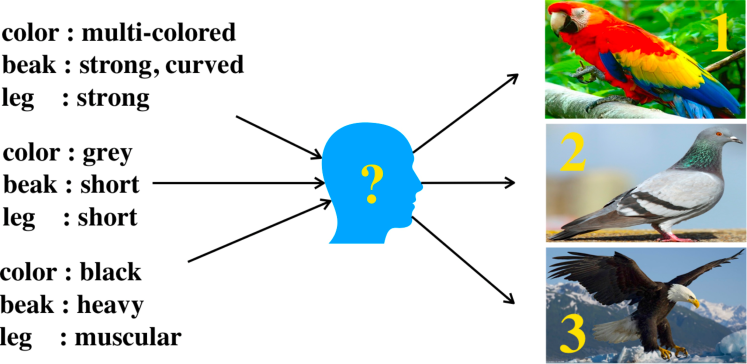
Figure 1: A simple scenario for zero-shot learning. It is easy for humans to transform the attribute information into mental pictures and choose the correct image. Can machines achieve this same level of intelligence?

Figure 2: Visualization of the refined attribute vector per class produced by APNet by using t-SNE (?) and the graph of classes generated based on given semantic embedding per class. The red nodes and blue nodes are the propagated attribute vectors for training classes and test classes, respectively. In the scatter plot, the attribute vectors of strongly-related classes are close to each other and these classes are connected by edges on the generated category graph (better viewed in color).

Zero-shot learning (ZSL) is a challenging task aiming to learn a model classifying images of any unseen classes given only the semantic attributes of the classes. It can test exactly the capability of generalizing knowledge learned on training classes to unseen classes, by establishing a scenario and asking a model to “imagine” the visual features of unseen classes (?) based on their semantic attributes. Generalized zero-shot learning (GZSL) assumes a more practical scenario. It is still based solely on semantic attributes of test classes with zero training sample, but the test set is composed of data from both seen and unseen classes, and the predictions are not restricted to the scope of unseen classes. The new challenge comes from the imbalance between seen and unseen classes and the possibility that the model mistakenly categorizes unseen class images as seen classes or vice versa. It requires the model to be easily adapted to unseen classes and meanwhile keeping its performance on seen/trained classes from degrading, while the potential problems could be: 1) the output prediction biases towards the seen/training class; and 2) the adapted model suffers from catastrophic forgetting of training classes.

The traditional supervised learning cannot work for ZSL due to the lack of training samples for unseen classes. However, even in such an extreme case, it is possible to derive visual patterns for images of unseen classes by exploring the relationship between unseen classes and seen classes, if given their semantic embeddings in the same attribute space, because an unseen class might share attributes with many seen classes. Hence, learning a classifier of unseen classes can be reduced to learning a transformation between the attribute space and the visual-feature space (?; ?) and a simple distance-based classifier can be generated for unseen classes in the attribute space. The method of learning a semantic-image transformation has been the most popular approaches for zero-shot learning during the past several years, and both linear (?) and nonlinear (?; ?) transformations have been studied.

In previous works, the attribute space is usually hand-crafted by human experts or pre-trained such as word embeddings of class names, and is independent to the zero-shot learning model. It is the only bridge relating unseen classes and the visual patterns learned for seen classes, so the quality and robustness of ZSL heavily rely on the attribute space. In addition, a pre-defined attribute space cannot fully capture the relationship between different classes which are most important to ZSL. In this paper, we optimize the attribute spaces and vectors by training an attribute propagation mechanism across a graph of classes together with the zero-shot classifier model in an end-to-end manner. Consequently, we can refine the attribute vectors of classes to be more informative in ZSL tasks by fully exploring the inter-class relations, which has not been rarely studied in previous works. The above strategy needs a graph of classes in advance. Fortunately, hierarchical structures and graph of categories are usually free or cheap to acquire in a variety of scenarios, e.g., the species in biology taxonomy, diseases in diagnostic and public heath systems, and merchandise on an e-commerce website.

In this paper, we aim to optimize the attribute space in the context of ZSL and leverage the inter-class relations to generate more powerful attribute vector per class. We propose “attribute propagation network (APNet)” as a neural nets model propagating the attributes of every class on the category graph to its neighbors in order to generate attribute vectors, followed by a nearest neighbor classifier with learnable similarity metric to produce prediction of an image based on its nearest neighbor among all classes’ attribute vectors in the learnable attribute space. The propagation updates attribute vector per class by a weighted sum of the attribute vectors of its neighboring classes on the graph. When the category graph is unavailable or inaccessible, we further reuse the attention module in propagation to generate a graph of classes given some pre-defined semantic embeddings of the classes. It computes similarity between classes in the semantic space and applies thresholding to the similarity values in order to determine whether adding an edge between two classes on the graph. All the above components can be trained together in an end-to-end manner on training classes and their samples. For better generalization on unseen classes and computational efficiency, we adopt a meta-learning strategy to train APNet on multiple randomly sampled subgraphs, each defining a classification task over the classes covered by the subgraph.

In experiments on five broadly-used benchmark datasets for ZSL, APNet achieves new state-of-the-art results in the practical generalized zero-shot learning setting and matches the current state-of-the-art results in the zero-shot learning setting. We further provide an ablation study of several possible variants of APNet, which show the effectiveness of our propagation mechanism and the improvements caused by the meta-learning training strategy.

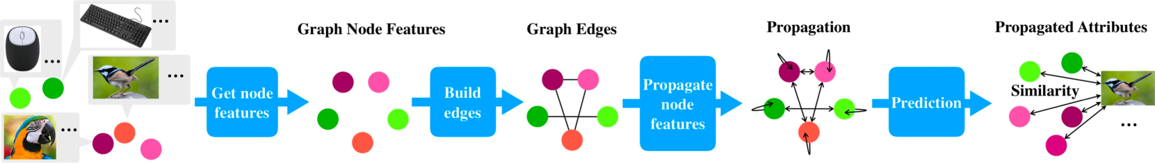
Figure 3: The pipeline of attribute propagation. 1. Initialize the nodes features: the attribute vectors of different classes are represented by different-colored dots. Each attribute vector is associated with some images from the corresponding class. The features of nodes on the propagation graph are initialized by transforming the attributes using the expert modules from (?). 2. Determine the graph edges: Two nodes on the propagation graph are connected by an edge if the similarity between their feature vectors exceeds a pre-determined threshold. 3. Propagation on the graph: The node features are propagated by an attention mechanism. 4. Zero-shot prediction: After propagation, a similarity metric is learned between the propagated context-aware/structure-aware attributes representations and a query image feature representation. The class with the largest similarity between the attribute vector after propagation and the query image’s embedding in the attribute space are regarded as the predicted class.

2 Related Work

Zero-shot learning (ZSL) (?; ?; ?) is an open problem that has been studied for a long time. Traditional methods learn a transformation between the semantic attribute space and visual-feature space (e.g., a hidden space of deep neural nets). In these works, given a learned similarity metric, ZSL is cast into a retrieval task, where the label is determined by retrieving the associated attributes from a set of candidate vectors based on the learned transformation (?; ?; ?; ?; ?; ?; ?). An implicit relationship between seen and unseen classes is that the properties of the unseen classes can be regarded as a mixture of properties of the seen classes. For example, a mixture of the semantic features of the seen classes (?) or a mixture of the weights of some phantom classes trained on the seen classes (?).

More recently, researchers start to integrate knowledge graph with zero-shot recognition (?; ?). They use graph convolutional network (GCN) which relies on a given knowledge graph to provide adjacency matrix and edges. In contrast, we use a modified graph attention network (GAN) (?; ?), which is capable to learn both the similarity metric and edges by itself even without any pre-defined graph or metric. Thereby, the propagation scheme learned in APNet is more powerful in modeling intra-task relationships and can be applied to more practical scenarios. For this reason, they cannot be applied to most ZSL benchmark datasets, which do not provide graphs. Their output of GCN is a fully connected layer per class, as a single-class classifier, that aims to approximate the corresponding part of the last layer of a pre-trained CNN, while our output of APNet is a prototype per class, from which we build a KNN classifier for each task. Hence, they need the CNN to be able to predict all the possible classes for all few-shot tasks. In contrast, we do not require any ground truth for the per-class classifier/prototype, so any pre-trained CNN can be used to provide features for APNet.

Our idea of attribute propagation is inspired by belief propagation, message passing and label propagation. It is also related to Graph Neural Networks (GNN) (?; ?), where convolution and attention are iteratively applied over a graph to construct node embeddings. In contrast to our work, their task is defined on graph-structured data, i.e., node classification (?), graph embedding (?), and graph generation (?). We only use the relationships between the categories/classes and build a computational graph that passes messages along the graph hierarchy. Our training strategy is inspired from the meta-learning training strategy proposed in (?), which have been broadly used in the meta-learning and few-shot learning literature (?; ?; ?), especially graph meta-learning (?; ?). However, this paper addresses zero-shot learning problem by training a novel model, i.e., APNet.

3 Problem Formulation

Zero-shot learning aims to learn a model that is generalizable to new classes or tasks whose semantic attributes are given but no training data is provided. For example, the model is expected to be applied to a classification task over some seen and unseen classes, The semantic attributes could have the form of an attribute vector, such as the main color of the class, or a word embedding of the class names.

Formally, we assume that a training set $\mathcal{X}^{tr}$ and a test set $\mathcal{X}^{te}$ are sampled from a data space $\mathcal{X}$. Each training data ${\bm{x}}\in\mathcal{X}^{tr}$ is annotated with a label $y\in\mathcal{Y}^{seen}$. The model is tested over $\mathcal{X}^{te}$, which are not only from the seen classes $\mathcal{Y}^{seen}$ but also the unseen classes $\mathcal{Y}^{unseen}$. The challenge is that the seen and unseen classes have no overlaps: $\mathcal{Y}^{seen}\cap\mathcal{Y}^{unseen}=\emptyset$. Hence, the semantic attributes ${\bm{S}}$ for each class is made available during both training and testing to act as a bridge between training classes and test classes. Specifically, every class $y\in\mathcal{Y}^{seen}\cup\mathcal{Y}^{unseen}$ is associated with a semantic embedding vector ${\bm{s}}_{y}\in{\bm{S}}$.

A direct mapping $F:\mathcal{X}\mapsto\mathcal{Y}$ from data to label is difficult to learn with zero-shot learning because the training and testing data are non-i.i.d. An alternative is to learn a mapping from data to the semantic attributes, i.e., $F:\mathcal{X}\mapsto{\bm{S}}$. In APNet, we learn a parameterized KNN classifier: the model learns a metric to measure the similarity between class-level semantic attributes and image representations. Here, the semantic attribute vector is a descriptor to the class label. Moreover, the higher the similarity, the higher the probability that the image belongs to the corresponding class. The hierarchical relationships between classes are incorporated into the semantic representations through an attribute propagation mechanism that traverses a graph. In the following sections, we will discuss how to build the propagation graph, how to propagate along it, and how to make predictions based on the propagated attribute representations.

4 Attribute Propagation Network

We propose the attribute propagation network (APNet) for zero-shot learning. APNet propagates attribute representations of each class between each other based on a semantic distance or class hierarchy, shared by both the seen classes and unseen classes, so that the propagated attribute representations can leverage the latent relationships between classes and generate context-aware/hierarchy-aware attribute representations. We learn a parametric KNN classifier since KNN classifier has better generality when the data is limited. The prediction in KNN depends on a learned similarity metric used to measure the discrepancy between the query image and the propagated semantic representation for each candidate class. The learned similarity is easier to generalize to the unseen classes based on the graph structure-encoded attribute representations. However, challenges still remain. In the rest of this section, we illustrate solutions to four of these challenges. 1. How to choose the nodes for the propagation graph? 2. How to represent the node features in the propagation graph? 3. How to find the edges in the propagation graph? 4. What is the best propagation mechanism?

4.1 Choosing the Graph Nodes

We assume propagation is built on a graph ${\mathcal{G}}=(\mathcal{Y},\mathcal{E})$, where each node $y\in\mathcal{Y}$ denotes a class, and each edge (or arc) $(y,z)\in\mathcal{E}$ connects two classes $y$ and $z$ and serves as a propagation pathway. Previous works built their propagation graph from a predefined class hierarchy (?; ?), e.g., the WordNet class hierarchy for ImageNet (?). In their approaches, each directed edge (or arc) $y\rightarrow z\in\mathcal{E}$ connects a parent class $y\in\mathcal{Y}$ to one of its child classes $z\in\mathcal{Y}$ on the graph ${\mathcal{G}}$. However, this kind of graph construction has some limitations: 1) It needs extra hierarchy information, which may not always be available; 2) The graph’s structure needs to be intact, and there needs to be a subgraph that covers all the targeted classification classes/nodes as well as their neighbors. A sparse graph containing neighbor nodes with many missing features would introduce noise when passing information through connected nodes, which might lead to a computational overhead that prevents the propagation being completed within a few steps. To flexibly apply graph propagation to classes regardless of how they are distributed in the actual class hierarchy, nodes with missing information are excluded from the propagation stage. In this way, the propagation process is not disturbed by those “blank” nodes uncovered by the training set.

4.2 Node Feature Representations

In this work, we assume that each node is associated with a feature representation. Encoded attributes for each class/node $y\in\mathcal{Y}$ are used for the initial node feature representations ${\bm{X}}_{y}^{0}$, following the model in (?):

$${\bm{X}}^{0}_{y}=\sum_{i=1}^{k}\operatorname*{ReLU}[\Theta_{i}({\bm{s}}_{y}-C_{i})],$$ (1)

where ${\bm{s}}_{y}\in{\bm{S}}$ is the provided side information, i.e., the class name embeddings for every class/node. ${\bm{C}}$ is the matrix for the centroids of the class attribute space, which is generated by $k$-means clustering and covers all training class attributes vectors ${\bm{S}}$. Each line ${\bm{C}}_{i}$ in the matrix stores one of the centroids. $\Theta_{i}$ is a linear transformation. We chose this model for its efficiency, since multiple attributes can share the encoding parameters $g_{i}$. Therefore, the number of parameters only grows linearly according to the number of centroids $|{\bm{C}}|$. Less learnable parameters can reduce problems with overfitting, which are common with zero-shot learning. Also, after encoding, the semantic information with different dimensions is unified so that the subsequent modules can use parameters of the same dimensions.

4.3 Finding the Graph Edges

As mentioned, the graph nodes are selected as a batch of nodes/classes that are available in the current task, with encoded class attributes as the node feature representation. Now we need to connect the nodes by deriving an adjacency matrix of the graph. An intuitive way to do this is to define a value in the adjacency matrix between node $i$ and node $j$ according to the predefined distance in the class hierarchy of the whole graph. For example, for the classes in ImageNet (?), each entry in adjacency matrix would be $A_{ij}=1/d_{ij}$, where the distance $d_{ij}$ is the number of hops between node $i$ and node $j$ on WordNet. (Note that we tried this type of adjacency matrix, and it generated similar results to APNet). Unfortunately, this kind of strategy requires extra information about the class hierarchy, e.g., WordNet. Hence, in our approach, we propose to generate the graph edges according to the node feature representations using an attention mechanism. More specifically, the attention learns a similarity metric $a(\cdot,\cdot)$ between node feature representation pairs and generates an edge between pairs with high similarity. The set of edges on graph $\mathcal{G}$ is:

$$\mathcal{E}=\left\{(y,z):y,z\in\mathcal{Y},a({\bm{X}}_{y}^{0},{\bm{X}}_{z}^{0})\geq\epsilon\right\},$$ (2)

$$a(p,q)\triangleq\frac{\langle f(p),f(q)\rangle}{\|f(p)\|_{2}\times\|f(q)\|_{2}},$$ (3)

where $f(\cdot)$ is a learnable transformation; and $\epsilon$ is a threshold for the similarity of the edge connection. For, simplicity, the edges are assumed to be undirected.

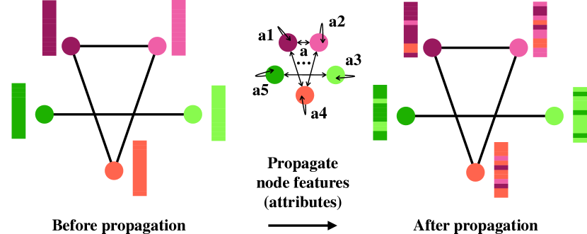
Figure 4: One-step of attribute propagation. Before propagation: The nodes, denoted by different-colored circles represent the different classes and the node features are the corresponding attribute feature representation of this class, denoted in the columns. The edges are generated based on the similarity between every node feature pair. Propagating the node features (attributes): Propagation computes a weighted sum of its neighbors’ node features, where the weights are produced by an attention module applied to every node feature and its neighbors (including itself). After-propagation: The attribute representations comprise a mixture of attribute representations from neighbors.

4.4 Attribute Propagation

The attribute propagation is based on the graph constructed in the previous subsections. The propagation is bidirectional through the edges using the learned attention mechanism. The node feature representations are a weighted sum of the features representations of its neighboring nodes $\mathcal{N}_{y}$, whose weights were obtained from the attention mechanism using Eq. (3). At step t, the propagation proceeds as follows:

$${\bm{X}}^{t+1}_{y}\leftarrow\sum_{z\in\mathcal{N}_{y}}a^{\prime}({\bm{X}}^{t}_{y},{\bm{X}}^{t}_{z})\times{\bm{X}}^{t}_{z},$$ (4)

where $a^{\prime}(\cdot,\cdot)$ is the normalized attention score over the neighbors $\mathcal{N}_{y}$ using softmax with hyper-parameter temperature $\gamma$ that controls the smoothness of the softmax function:

$$a^{\prime}({\bm{X}}^{t}_{y},{\bm{X}}^{t}_{z})=\frac{\exp[\gamma_{1}a({\bm{X}}^{t}_{y},{\bm{X}}^{t}_{z})]}{\sum_{z\in\mathcal{N}_{y}}\exp[\gamma_{1}a({\bm{X}}^{t}_{y},{\bm{X}}^{t}_{z})]}.$$ (5)

The propagation can be applied multiple times to collect messages from indirectly-connected neighbors and, in so doing, amass a more comprehensive understanding of the graph structure. Figure 4 shows an example of one-step propagation.

4.5 Parameterized KNN for Prediction

In this approach, we learn a similarity metric between an attribute representation and a query image representation as the parametric KNN. A learned metric calculates the similarity between the $t$-th step propagated attribute matrix ${\bm{X}}^{t+1}$ and the query image feature vectors. Inspired by the concept of additive attention  (?), the similarity between an image with feature ${\bm{x}}$ and class $y$ is:

$$h({\bm{X}}^{t+1}_{y},{\bm{x}})={\bm{w}}\sigma^{(1)}({\bm{W}}^{(1)}{\bm{X}}^{t+1}_{y}+{\bm{W}}^{(2)}{\bm{x}}+{\bm{b}}^{(1)})+b,$$ (6)

where ${\bm{W}}^{(1)}$, ${\bm{W}}^{(2)}$, ${\bm{b}}$, ${\bm{w}}$ and $b^{(1)}$ are learnable parameters, and $\sigma^{(1)}$ is a nonlinear activation function. The class whose propagated attribute vector with the highest similarity to the image vector is taken as the final prediction. The probability of predicting ${\bm{x}}$ as class $y$ normalized with temperature $\gamma_{2}$ over a batch of classes $\mathcal{Y}^{T}$ is:

$$\Pr(y|{\bm{x}};{\bm{X}}^{t+1})=\frac{\exp(\gamma_{2}h({\bm{X}}^{t+1}_{y},{\bm{x}}))}{\sum_{z\in\mathcal{Y}^{T}}\exp(\gamma_{2}h({\bm{X}}^{t+1}_{z},{\bm{x}}))}.$$ (7)

We assume that the attribute propagation does not affect the associated attribute labels so the label for the propagated attributes is the same as the original associated label before propagation, i.e., ${\bm{X}}^{t}_{y}$ is the attribute for class $y$ before propagation while the ${\bm{X}}^{t+1}_{y}$ is still the attribute for class $y$ after propagation.

4.6 Training Strategy and Scalability

Training APNet over all the nodes/classes in a dataset would be too computationally expensive since the size of the attention score matrix grows exponentially as the number of nodes/classes grows. Moreover, applying a cost constraint over the loss computation may make the optimization unstable. Hence, for training efficiency, we only sample a subgraph to apply the propagation per iteration. Additionally, to improve the generality of our model to unseen nodes/classes, we train APNet on different classification tasks in every iteration, so it can quickly adapt to different new tasks. This technique was inspired by the training strategy of meta-learning originally developed for few-shot learning in (?). The aim of few-shot learning is to build a model that can adapt quickly to any new task with only a few training samples. In contrast, the goal of zero-shot learning is to learn a model that can generalize to a new task with only the semantic information provided. However, we found the idea of meta-learning training strategy designed for “fast adaptability” could also improve the generality of our model. Interestingly, this training strategy might also benefit other models in the literature of zero-shot learning.

In every iteration, a task $T$ is sampled from a task distribution ${\mathcal{T}}$. The aim is to minimize the loss for this classification task based on our APNet model. The training objective is to minimize the empirical risk:

$$\min_{\Theta}{{\mathbb{E}}}_{T\sim{\mathcal{T}}}{{\mathbb{E}}}_{({\bm{x}},y)\sim{\mathcal{D}}^{T}}-\log\Pr(y|{\bm{x}};{\bm{X}}^{T}),$$ (8)

where each task $T$ is defined as a subset of classes $\mathcal{Y}^{T}\subseteq\mathcal{Y}^{seen}$; $\mathcal{D}^{T}$ is the distribution of data-label pair $({\bm{x}},y)$ with $y\in\mathcal{Y}^{seen}$; ${\bm{X}}^{T}$ is the corresponding propagated attributes matrix for classes in task $T$; $\Theta$ are the learnable parameters.

Table 1: Datasets Statistics. “#*” denotes the number of *. “Tr-S”, “Te-S” and “Te-U” denotes seen classes in training, seen classes in test and unseen classes in test, respectively.

Dataset	Granularity	#Attributes	#Seen classes	#Unseen classes	#Imgs(Tr-S)	#Imgs(Te-S)	#Imgs(Te-U)
SUN	fine	102	645	72	10,320	2,580	1,440
CUB	fine	312	150	50	7,057	1,764	2,967
AWA1	coarse	85	40	10	19,832	4,958	5,685
AWA2	coarse	85	40	10	23,527	5,882	7,913
aPY	coarse	64	20	12	5,932	1,483	7,924

Table 2: Performance comparisons for generalized zero-shot learning between our method and baselines on five datasets, where “S” denotes per-class accuracy (%) for seen classes, “U” denotes per-class accuracy (%) for unseen classes and “H” denotes harmonic mean of “S” and “U”. Parts of the results are from (?).

Methods	SUN			CUB			AWA1			AWA2			aPY
	S	U	H	S	U	H	S	U	H	S	U	H	S	U	H
DEVISE (?)	27.4	16.9	20.9	53.0	23.8	32.8	68.7	13.4	22.4	74.7	17.1	27.8	76.9	4.9	9.2
CONSE (?)	39.9	6.8	11.6	72.2	1.6	3.1	88.6	0.4	0.8	90.6	0.5	1.0	91.2	0.0	0.0
SYNC (?)	43.3	7.9	13.4	70.9	11.5	19.8	87.3	8.9	16.2	90.5	10.00	18.0	66.3	7.4	13.3
SAE (?)	18.0	8.8	11.8	54.0	7.8	13.6	77.1	1.8	3.5	82.2	1.1	2.2	80.9	0.4	0.9
DEM (?)	34.3	20.5	25.6	57.9	19.6	29.2	84.7	32.8	47.3	86.4	30.5	45.1	75.1	11.1	19.4
RN (?)	-	-	-	61.1	38.1	47.0	91.3	31.4	56.7	93.4	30.0	45.3	-	-	-
PQZSL (?)	35.3	35.1	35.2	51.4	43.2	46.9	70.9	31.7	43.8	-	-	-	64.1	27.9	38.8
CRNet (?)	36.5	34.1	35.3	56.8	45.5	50.5	74.7	58.1	65.4	78.8	52.6	63.1	68.4	32.4	44.0
APNet(ours)	40.6	35.4	37.8	55.9	48.1	51.7	76.6	59.7	67.1	83.9	54.8	66.4	74.7	32.7	45.5

5 Experiments

5.1 Datasets

We used five widely-used zero-shot learning datasets in our experiments: AWA1 (?), AWA2 (?), SUN (?), CUB (?) and aPY (?). To avoid overlaps between the test sets and ImageNet-1K, which is used for pretraining backbones, we followed the splits proposed in (?). AWA1, AWA2 and CUB are subsets of ImageNet. AWA1 and AWA2 have 50 animals classes with pre-extracted feature representations for each image. CUB is also a subset of ImageNet with images of 200 bird species (mostly North American). SUB is a Scene benchmark containing 397 scene categories. aPY is a small dataset including 32 classes. Detailed statistics are provided in Table 1.

5.2 Implementation Details

For a fair comparison with baselines, we followed (?)’s implementation and used a pre-trained ResNet-101 (?) on ImageNet-1K to extract 2048-dimensional image features with no fine-tuning on the backbone. We trained our APNet with Adam (?) for 360 epochs with weight decay factor of 0.0001. The initial learning rate was 0.00002 with a decrease of 0.1 every 240 epochs. The number of iterations in every epoch under an $N$-way-$K$-shot training strategy was $\|\mathcal{X}^{tr}\|/NK$, where $N$ was 30 and $K$ was 1 in our exeperiments. The temperature $\gamma_{1}$ was 10 and $\gamma_{2}$ was 30. Transformation functions $g_{i}$ and $f$ were linear transformations. The threshold for connecting edges was set to $\textrm{cosine}40^{o}~{}\approx~{}0.76$. All nonlinear functions were ReLU except for $\sigma$, which was implemented using Sigmoid to map the result between 0 and 1.

Table 3: Per-class accuracy (%) comparisons over unseen classes for zero-shot learning between our method and baselines on five datasets. Parts of the results are from (?).

Methods	SUN	CUB	AWA1	AWA2	aPY
DEVISE (?)	56.5	52.0	54.2	59.7	39.8
ALE (?)	58.1	54.9	59.9	62.5	39.7
SYNC (?)	56.3	55.6	54.0	46.6	23.9
SAE (?)	40.3	33.3	53.0	54.1	8.3
RN (?)	-	55.6	68.2	64.2	-
GAFE (?)	62.2	52.6	67.9	67.4	44.3
APNet(ours)	62.3	57.7	68.0	68.0	41.3

5.3 Evaluation Criterion

To mitigate the bias caused by imbalance of test data for every class, following the most recent works (?), we evaluate the APNet’s performance according to averaged per-class accuracy:

$$ACC_{\mathcal{Y}}= \frac{1}{|\mathcal{Y}|}\sum_{y\in\mathcal{Y}}\frac{1}{|D_{y}|}\sum_{({\bm{x}},y)\in D_{y}}\mathbbm{1}[\widehat{y}=y],$$ (9)

where $\mathcal{D}_{y}$ is the dataset of the data-label pairs for class $y$, and $\widehat{y}$ is the prediction of the image feature representation ${\bm{x}}$. We measured the overall accuracy of the data in the seen and unseen classes in terms of the harmonic mean of the per-class seen accuracy $ACC_{\mathcal{Y}^{seen}}$ and unseen accuracy $ACC_{\mathcal{Y}^{unseen}}$ following previous works (?): $H=\frac{2*ACC_{\mathcal{Y}^{seen}}*ACC_{\mathcal{Y}^{unseen}}}{ACC_{\mathcal{Y}^{seen}}+ACC_{\mathcal{Y}^{unseen}}}$.

5.4 Experimental Results

Generalized Zero-shot Learning.

With generalized zero-shot learning, the setting is to classify samples (${\bm{x}}$, $y\in\mathcal{Y}^{seen}\cup\mathcal{Y}^{unseen}$) from both seen and unseen classes while training on samples (${\bm{x}}$, $y\in\mathcal{Y}^{seen}$) from seen classes. The comparison results for APNet and other baselines are shown in Table 2.

Classical zero-shot learning methods, e.g., CMT, CONSE, usually suffer from the imbalance problem between the training and testing stages. Their models perform well on the seen classes but the per-class accuracy on the unseen classes is low, with some models even achieving close to 0% per-class accuracy. It is challenging to achieve competitive results on every dataset for the generalized zero-shot learning due to the imbalanced accuracy for seen classes and unseen classes because of model overfitting to samples from the seen classes. Our APNet outperforms state-of-the-art results on all five datasets. Our model achieves better results especially on datasets extracted from ImageNet, i.e., CUB, AWA1, AWA2, and achieves over 3 points improvements on the overall criterion ($H$) for both seen and unseen accuracy, and consistent improvements on the unseen accuracy of up to $\sim 3\%$.

Zero-shot Learning.

The setting with zero-shot learning is to classify samples (${\bm{x}}$, $y\in\mathcal{Y}^{unseen}$) from unseen classes while training on samples (${\bm{x}}$, $y\in\mathcal{Y}^{seen}$) from seen classes. The comparison results for APNet and the other baselines are shown in Table 3. APNet achieves competitive results in this setting. Similar to the results in GZSL, APNet is more powerful on subsets of ImageNet datasets, i.e., CUB, AWA1, AWA2, where APNet achieves up to $2\%$ accuracy improvements compared to the most recent baselines.

Comparing the results for both generalized zero-shot learning in Table 2 and zero-shot learning in Table 3 settings, it is challenging to perform well on both settings. Methods that perform well on zero-shot learning do not guarantee a good performance on generalized zero-shot learning. DEM (?) achieved similar performance compared to our APNet on AWA1. However, the generalization ability of DEM, which is measured by the performance in the setting of generalized zero-shot learning, has space for improvements. This is probably because DEM treats visual space as the embedding space for nearest neighbor search. Comparatively, we mainly do transformation over the semantic embeddings by propagation on a shared graph of training and test classes and use a parametric KNN classifier for a semantic-visual joint similarity prediction. The visual space used in DEM has high bias and non-i.i.d. problems and might be difficult to generalize when considering predictions over both seen classes and unseen classes. GAFE (?) achieved better performance on aPY dataset but also suffers from the generalization ability problem. Similar to DEM, they also focused on the visual space and proposed a reconstruction regularizer on the visual feature representations. In remains open if the regularizer can generalize on the unseen classes without their visual feature representations during training stage.

Ablations and Variants of APNet.

We did ablation study and developed some variants of APNet in Table 4. In the ablation of propagation ($\times$ in “Graph Hierarchy”), we skip the propagation step and directly use the node feature representations for similarity comparison and prediction. Propagation can achieve above $1$ point improvement on $H$ under different training strategies.

Two variants of APNet are developed by adjusting the training strategy to traditional minibatch training (denoted by $\times$ in “Meta training”) and replacing the graph hierarchy used in propagation with the hierarchy defined in WordNet. The meta-learning style training strategy we used can bring $2\sim 3\%$ accuracy improvements on unseen accuracy and $2\sim 3$ points improvement on $H$ while keeping the rest components the same, which verifies that training on different tasks in every iteration can get better model generality. When the hierarchy is defined by WordNet, the propagation graph is assumed to be fully connected and the value of the adjacency matrix for node $i$ and node $j$ ($A_{ij}$) is defined as $1/d_{ij}$, where $d_{ij}$ is the number of hops between node $i$ and node $j$ on WordNet. Predefined graph hierarchy can bring improvements but is sensitive to the training strategy. The reason is probably that the exact/optimal formulation for generating the adjacency matrix based on the distance between nodes is unclear even though intuitively closer nodes should have higher values for its adjacency matrix. Dedicated designs on how to integrate the hierarchy information more effectively have the potential to boost the performance.

Table 4: Ablations and performance comparisons on variants of APNet on AWA2.

Meta Training	Graph Hierarchy	S	U	H
$\times$	$\times$	82.8	50.2	62.5
$\times$	WordNet	83.9	50.4	62.9
$\times$	Learned	81.2	52.6	63.9
$\checkmark$	$\times$	84.4	53.4	65.4
$\checkmark$	WordNet	82.6	55.7	66.6
$\checkmark$	Learned	83.9	54.8	66.4

6 Acknowledgments

This research was funded by the Australian Government through the Australian Research Council (ARC) under grants 1) LP160100630 partnership with Australia Government Department of Health and 2) LP180100654 partnership with KS Computer. We also acknowledge the support of NVIDIA Corporation and Google Cloud with the donation of GPUs and computation credits.

References

- [Akata et al. 2015a] Akata, Z.; Perronnin, F.; Harchaoui, Z.; and Schmid, C. 2015a. Label-embedding for image classification. T-PAMI.
- [Akata et al. 2015b] Akata, Z.; Reed, S.; Walter, D.; Lee, H.; and Schiele, B. 2015b. Evaluation of output embeddings for fine-grained image classification. In CVPR.
- [Changpinyo et al. 2016] Changpinyo, S.; Chao, W.-L.; Gong, B.; and Sha, F. 2016. Synthesized classifiers for zero-shot learning. In CVPR.
- [Dai et al. 2018] Dai, H.; Tian, Y.; Dai, B.; Skiena, S.; and Song, L. 2018. Syntax-directed variational autoencoder for structured data. In ICLR.
- [Deng et al. 2009] Deng, J.; Dong, W.; Socher, R.; Li, L.-J.; Li, K.; and Fei-Fei, L. 2009. ImageNet: A large-scale hierarchical image database. In CVPR.
- [Dong and Yang 2019] Dong, X., and Yang, Y. 2019. Searching for a robust neural architecture in four gpu hours. In CVPR.
- [Farhadi et al. 2009] Farhadi, A.; Endres, I.; Hoiem, D.; and Forsyth, D. 2009. Describing objects by their attributes. In CVPR.
- [Finn, Abbeel, and Levine 2017] Finn, C.; Abbeel, P.; and Levine, S. 2017. Model-agnostic meta-learning for fast adaptation of deep networks. In ICML.
- [Frome et al. 2013] Frome, A.; Corrado, G. S.; Shlens, J.; Bengio, S.; Dean, J.; Mikolov, T.; et al. 2013. Devise: A deep visual-semantic embedding model. In NeurIPS.
- [Hamilton, Ying, and Leskovec 2017] Hamilton, W.; Ying, Z.; and Leskovec, J. 2017. Inductive representation learning on large graphs. In NeurIPS.
- [He et al. 2016] He, K.; Zhang, X.; Ren, S.; and Sun, J. 2016. Deep residual learning for image recognition. In CVPR.
- [Henaff, Bruna, and LeCun 2015] Henaff, M.; Bruna, J.; and LeCun, Y. 2015. Deep convolutional networks on graph-structured data. arXiv preprint arXiv:1506.05163.
- [Kampffmeyer et al. 2019] Kampffmeyer, M.; Chen, Y.; Liang, X.; Wang, H.; Zhang, Y.; and Xing, E. P. 2019. Rethinking knowledge graph propagation for zero-shot learning. In CVPR.
- [Kingma and Ba 2015] Kingma, D. P., and Ba, J. 2015. Adam: A method for stochastic optimization. In ICLR.
- [Kodirov, Xiang, and Gong 2017] Kodirov, E.; Xiang, T.; and Gong, S. 2017. Semantic autoencoder for zero-shot learning. In CVPR.
- [Lampert, Nickisch, and Harmeling 2014] Lampert, C. H.; Nickisch, H.; and Harmeling, S. 2014. Attribute-based classification for zero-shot visual object categorization. T-PAMI.
- [Larochelle, Erhan, and Bengio 2008] Larochelle, H.; Erhan, D.; and Bengio, Y. 2008. Zero-data learning of new tasks. In IJCAI.
- [Li et al. 2019] Li, J.; Lan, X.; Liu, Y.; Wang, L.; and Zheng, N. 2019. Compressing unknown images with product quantizer for efficient zero-shot classification. In CVPR.
- [Liu et al. 2019a] Liu, L.; Zhou, T.; Long, G.; Jiang, J.; Yao, L.; and Zhang, C. 2019a. Prototype propagation networks (PPN) for weakly-supervised few-shot learning on category graph. IJCAI.
- [Liu et al. 2019b] Liu, L.; Zhou, T.; Long, G.; Jiang, J.; and Zhang, C. 2019b. Learning to propagate for graph meta-learning. In NeurIPS.
- [Liu et al. 2019c] Liu, Y.; Xie, D.; Gao, Q.; Han, J.; Wang, S.; and Gao, X. 2019c. Graph and autoencoder based feature extraction for zero-shot learning. In IJCAI.
- [Maaten and Hinton 2008] Maaten, L. v. d., and Hinton, G. 2008. Visualizing data using t-SNE. JMLR.
- [Norouzi et al. 2013] Norouzi, M.; Mikolov, T.; Bengio, S.; Singer, Y.; Shlens, J.; Frome, A.; Corrado, G. S.; and Dean, J. 2013. Zero-shot learning by convex combination of semantic embeddings. NeurIPS.
- [Pan et al. 2018] Pan, S.; Hu, R.; Long, G.; Jiang, J.; Yao, L.; and Zhang, C. 2018. Adversarially regularized graph autoencoder for graph embedding. In IJCAI, 2609–2615.
- [Patterson and Hays 2012] Patterson, G., and Hays, J. 2012. Sun attribute database: Discovering, annotating, and recognizing scene attributes. In CVPR.
- [Romera-Paredes and Torr 2015] Romera-Paredes, B., and Torr, P. 2015. An embarrassingly simple approach to zero-shot learning. In ICML.
- [Santoro et al. 2016] Santoro, A.; Bartunov, S.; Botvinick, M.; Wierstra, D.; and Lillicrap, T. 2016. Meta-learning with memory-augmented neural networks. In ICML.
- [Shen et al. 2018] Shen, T.; Zhou, T.; Long, G.; Jiang, J.; Pan, S.; and Zhang, C. 2018. Disan: Directional self-attention network for rnn/cnn-free language understanding. In AAAI.
- [Shen et al. 2019] Shen, T.; Zhou, T.; Long, G.; Jiang, J.; and Zhang, C. 2019. Tensorized self-attention: Efficiently modeling pairwise and global dependencies together. In NAACL-HLT.
- [Snell, Swersky, and Zemel 2017] Snell, J.; Swersky, K.; and Zemel, R. 2017. Prototypical networks for few-shot learning. In NeurIPS.
- [Socher et al. 2013] Socher, R.; Ganjoo, M.; Manning, C. D.; and Ng, A. 2013. Zero-shot learning through cross-modal transfer. In NeurIPS.
- [Sung et al. 2018] Sung, F.; Yang, Y.; Zhang, L.; Xiang, T.; Torr, P. H.; and Hospedales, T. M. 2018. Learning to compare: Relation network for few-shot learning. In CVPR.
- [Vaswani et al. 2017] Vaswani, A.; Shazeer, N.; Parmar, N.; Uszkoreit, J.; Jones, L.; Gomez, A. N.; Kaiser, Ł.; and Polosukhin, I. 2017. Attention is all you need. In NeurIPS.
- [Vinyals et al. 2016] Vinyals, O.; Blundell, C.; Lillicrap, T.; Wierstra, D.; et al. 2016. Matching networks for one shot learning. In NeurIPS.
- [Wang et al. 2017] Wang, C.; Pan, S.; Long, G.; Zhu, X.; and Jiang, J. 2017. Mgae: Marginalized graph autoencoder for graph clustering. In CIKM.
- [Wang, Ye, and Gupta 2018] Wang, X.; Ye, Y.; and Gupta, A. 2018. Zero-shot recognition via semantic embeddings and knowledge graphs. In CVPR.
- [Welinder et al. 2010] Welinder, P.; Branson, S.; Mita, T.; Wah, C.; Schroff, F.; Belongie, S.; and Perona, P. 2010. Caltech-ucsd birds 200. Technical report, California Institute of Technology.
- [Wu et al. 2019] Wu, Z.; Pan, S.; Chen, F.; Long, G.; Zhang, C.; and Yu, P. S. 2019. A comprehensive survey on graph neural networks. arXiv preprint arXiv:1901.00596.
- [Xian et al. 2016] Xian, Y.; Akata, Z.; Sharma, G.; Nguyen, Q.; Hein, M.; and Schiele, B. 2016. Latent embeddings for zero-shot classification. In CVPR.
- [Xian et al. 2019] Xian, Y.; Lampert, C. H.; Schiele, B.; and Akata, Z. 2019. Zero-shot learning-a comprehensive evaluation of the good, the bad and the ugly. T-PAMI.
- [Xie et al. 2019] Xie, G.-S.; Liu, L.; Jin, X.; Zhu, F.; Zhang, Z.; Qin, J.; Yao, Y.; and Shao, L. 2019. Attentive region embedding network for zero-shot learning. In CVPR.
- [Zhang and Shi 2019] Zhang, F., and Shi, G. 2019. Co-representation network for generalized zero-shot learning. In ICML.
- [Zhang, Xiang, and Gong 2017] Zhang, L.; Xiang, T.; and Gong, S. 2017. Learning a deep embedding model for zero-shot learning. In CVPR.