A new multivariate meta-analysis model for many variates and few studies

Abstract

Studies often estimate associations between an outcome and multiple variates. For example, studies of diagnostic test accuracy estimate sensitivity and specificity, and studies of predictive and prognostic factors typically estimate associations for multiple factors. Meta-analysis is a family of statistical methods for synthesizing estimates across multiple studies. Multivariate models exist that account for within-study correlations and between-study heterogeneity. The number of parameters that must be estimated in existing models is quadratic in the number of variates (e.g., risk factors). This means they may not be usable if data are sparse with many variates and few studies. We propose a new model that addresses this problem by approximating a variance-covariance matrix that models within-study correlation and between-study heterogeneity in a low-dimensional space using random projection. The number of parameters that must be estimated in this model scales linearly in the number of variates and quadratically in the dimension of the approximating space, making estimation more tractable. We performed a simulation study to compare coverage, bias, and precision of estimates made using the proposed model to those from univariate meta-analyses. We demonstrate the method using data from an ongoing systematic review on predictors of pain and function after total knee arthroplasty. Finally, we suggest a decision tool to help analysts choose among available models.

Keywords multivariate random-effects meta-analysis; missing data; sparsity; Bayesian statistics; random projection

Git revision 72ca65b

Introduction

Meta-analysis is a family of statistical methods used to synthesize estimates of one or more common variates reported by multiple studies [2]. The aim is to obtain a single estimate that statistically characterizes the totality of the available evidence, often including any between-study heterogeneity. For example, a variate of interest might be the prevalence of a particular disease, or a risk ratio comparing a treatment to a comparator. As in the examples, the most commonly-used meta-analysis models are univariate, which means that each primary study contributes an estimate of a single variate. Univariate meta-analysis is not necessarily appropriate if there are multiple variates. While it may be tempting to apply univariate meta-analysis to each variate separately, this does not account for possible correlations between variates and does not allow “borrowing of strength” across variates and studies [6]. Univariate meta-analyses applied in the multivariate setting are expected to provide excessively biased and imprecise estimates [16].

The alternative is multivariate meta-analysis, which in principle can model all variates of interest, as well as any within-study correlation and between-study heterogeneity, simultaneously. Perhaps the most well-known application of multivariate meta-analysis within biomedical research is in studying diagnostic test accuracy (DTA), in which the variates sensitivity and specificity are of interest [8]. It is generally recognized that univariate meta-analysis is inappropriate for DTA because changing the threshold that distinguishes positive from negative test results to increase sensitivity will typically decrease specificity. This correlation between sensitivity and specificity is not modeled by univariate meta-analyses. Multivariate meta-analysis is also of use in the study of predictive and prognostic factors, in which a given outcome may be associated with more than one factor. Network meta‐analysis (multiple treatment comparison) can also be posed as multivariate meta-analysis [22]. In addition to the challenges faced in univariate meta-analysis, the multivariate setting poses additional ones, some or all of which may be addressed by available methods:

1. It is rare for authors of primary studies to report an estimate of the full variance-covariance or correlation matrix.

2. It cannot be assumed that every primary study provides estimates for all variates of interest.

3. As in univariate meta‐analysis, it is typical to observe between-study heterogeneity in the estimates.

A further challenge, addressed herein, is the scenario in which the number of variates (e.g., prognostic factors) is large relative to the number of primary studies. It may not be possible to use existing multivariate meta-analysis models in such circumstances because the number of parameters needed to estimate within‐study correlation and between-study heterogeneity is quadratic in the number of variates. Our contribution is to use a low-dimensional variance-covariance matrix that approximates common within‐study correlation and between-study heterogeneity. We do this using a dimensionality reduction method called random projection [12, 5]. This allows us to reduce the number of parameters that must be estimated to be linear in the number of variates. Estimation is thereby more tractable when there are few studies and many variates.

This paper begins with a motivating example from an ongoing systematic review of predictive factors in which existing methods could not be used. We then provide mathematical background on multivariate meta-analytical methods and explain in more detail why estimation is challenging when there are many variates and few studies. We introduce our model and present a simulation study that compares the proposed method to univariate meta-analysis with respect to bias, variance, and coverage probability. We close with a discussion that presents a decision aid for choosing among the models considered herein, and suggest avenues for future research.

Motivating example

This work was motivated by an ongoing systematic review of factors that may predict chronic pain and physical function after total knee arthroplasty (TKA) [14]. About 20% of patients who undergo TKA experience post-surgical pain and reduced function [1], and numerous factors have been studied. Being able to characterize factors predictive of post-surgical pain could lead to better health outcomes and resource use. Following the inclusion criteria specified in our protocol, we extracted or imputed 38 estimates of correlation coefficients between 23 predictors and six-month post-surgical pain (a prespecified secondary outcome) from 7 studies that included a total of 5473 patients (approximately 2700 patient-years of follow-up). We had planned to perform multivariate meta-analysis using an extension of the common correlation model of Riley et al. [15], as implemented in the MVMETA add-on command for Stata [20, 21]. However, because the extracted data are sparse, it was not possible to perform the prespecified analysis unless we applied some criterion to limit the number of studies and predictors included in the analysis. We found that including predictors supported by at least four studies allowed the prespecified model to be used. However, this approach has at least two clear problems. First, the choice of criterion represents an investigator degree of freedom, and it is possible that several other reasonable criteria would each allow the model to be fitted, likely yielding differing results. Second, the criterion we chose limited the number of predictors for which multivariate meta-analysis estimates could be obtained to just two (see figure 1). Recognizing that the planned analysis was suboptimal, we then attempted to use Lin and Chu’s model [13], which was developed to address the problem of sparse data in multivariate meta-analysis. Unfortunately, the available data were also too sparse to support this model.

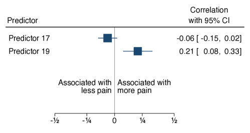
Figure 1: Multivariate meta-analysis could only be performed for two of the 23 predictors using the model of Riley et al.

Background

Let $\mathbb{S}$ be a set of $m$ studies. The $i$-th study provides $1\leq t_{i}\leq p$ point estimates and sampling variances, where $p$ is the total number of unique variates studied. Let the point estimates provided by study $i$ be denoted $y_{i}\in\mathbb{R}^{t_{i}}$ and the corresponding diagonal matrix of sampling variances be denoted $D_{i}\in\mathbb{R}_{\geq 0}^{t_{i}\times t_{i}}$. Given the $y_{i}$ and $D_{i}$, we wish to estimate the true value of the $p$ variates, $\mu\in\mathbb{R}^{p}$, accounting for within‐study correlation and between-study heterogeneity. We assume that none of the studies report within-study correlation or variance-covariance matrices.

Riley et al. [15] proposed a bivariate meta-analysis model that assumes a common within-study correlation parameter. A multivariate version of this model has been implemented for Stata by White [20, 21]. Assuming such a model is parameterized in terms of a common within-study correlation matrix and a between-study variance-covariance matrix that models heterogeneity, the parameters to be estimated are the $p$ elements of $\mu$, the $\frac{1}{2}p(p-1)$ elements of the common within-study correlation matrix (which is unitriangular), and the $\frac{1}{2}p(p+1)$ elements of the upper or lower triangle of the variance-covariance matrix that models heterogeneity. Such a model requires a total of $p^{2}+p$ parameters to be estimated. It may be challenging to fit such a model unless the total number of point estimates provided by the studies $n=\sum_{i\in\mathbb{S}}t_{i}\geq p^{2}+p$. For many research questions, sufficient studies and estimates may not exist, particularly if $p$ is large. We say the problem is sparse if $n<p^{2}+p$.

Lin and Chu [13] developed on the model of Riley et al. and addressed the sparsity problem by modeling the variance-covariance matrix for each study as a sum of sampling and additional variances, and by assuming a common correlation matrix for all $p$ variates. Their model requires estimating the $p$ elements of $\mu$, the $p$ additional variances, and the $\frac{1}{2}p(p-1)$ correlations, for a total of $\frac{1}{2}p(p+3)$ parameters.

Model	Number of Parameters
Riley et al.	$p^{2}+p$
Lin and Chu	$\frac{1}{2}p(p+3)$
Our Model	$p+\frac{1}{2}q(q-1)$

Table 1: The number of parameters that must be estimated for each model; $p$ is the total number of variates across all studies, and $q$ is the dimensionality of the space in which within-study correlation and between-study heterogeneity are modeled.

A low-dimensional model

As in previous work, we make the simplifying assumptions that variates not estimated by particular studies are missing completely at random, and have a common correlation structure across the primary studies [13, 15]. We develop on Lin and Chu’s model by assuming that the within-study correlation structure and between-study heterogeneity are well approximated in a low-dimensional space. This allows us to reduce the number of parameters that must be estimated. Our model is:

$$y_{i}\sim\mathcal{N}(X_{i}\mu,\Phi_{i})\textrm{ for }i\in\mathbb{S}$$ (1)

where

$$\Phi_{i}=D_{i}+X_{i}R^{\top}\Sigma RX_{i}^{\top}$$ (2)

$X_{i}$ is a $t_{i}\times p$ indicator matrix. Its $(j,k)$-th element is unity if the $j$-th estimate reported by the $i$-th study corresponds to the $k$-th of the $p$ variates and is zero otherwise. $R\in\mathbb{R}^{q\times p}$ is a matrix that maps between the full $p$-dimensional space and a $q$-dimensional space (where $q<p$) in which the full within- and between-study variance-covariance matrix is approximated by the symmetric positive-definite matrix $\Sigma\in\mathbb{R}^{q\times q}$. Table 1 summarizes the number of parameters that must be estimated by the models of Riley et al., Lin and Chu, and our model. In brief, for fixed $q$ (which would reasonably be in the range 2–10), the number of parameters that must be estimated for our model scales as $O(p)$ rather than $O(p^{2})$, as for those of Riley et al. and Lin and Chu. Figure 2 plots number of model parameters as a function of number of variates for Riley’s and Lin and Chu’s models, and our model with $q=4$ and $q=8$.

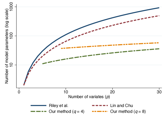
Figure 2: Number of model parameters as a function of number of variates for Riley’s and Lin and Chu’s models, and our model with $q=4$ and $q=8$. Curves for our model are shown for $q<p$.

We use a random projection matrix [5, 9] for $R$, but any suitable dimensionality-reduction method could be used instead. There is a large literature on the theory and applications of random projection, and [5] provides a good introduction. The following is a brief and informal treatment of the relevant concepts. Further background on the approach is provided in the Discussion section.

Recall that an orthogonal linear transformation matrix $T\in\mathbb{R}^{p\times p}$ maps between orthonormal bases and preserves the magnitudes and angles between vectors. Such transforms are of interest in multivariate statistics, in particular in principal component analysis (PCA), which has application in dimensionality reduction. Briefly, PCA can be posed as follows: given a variance-covariance matrix $\Lambda$, find matrix $T$ such that $T\Lambda{}T^{\top}$ is a diagonal matrix of variances that preserves the total variance of $\Lambda$. This can be achieved via eigendecomposition of $\Lambda$, giving a matrix of eigenvectors ($T$) and their associated eigenvalues, the latter of which provide information about the proportion of the total variance explained in the direction of each of the eigenvectors. Dimensionality reduction can be achieved via the matrix $T^{\prime}\in\mathbb{R}^{q\times p}$, with $q<p$. $T^{\prime}$ is formed by dropping those eigenvectors from $T$ that have the smallest associated eigenvalues. Hence, a dimensionality-reducing transform can be defined that preserves at least a given proportion of the total variance. In short, the original matrix $\Lambda$ can be approximated in a $q$-dimensional space by $T^{\prime}\Lambda{}T^{\prime\top}$.

PCA is only applicable if the variance-covariance matrix is known or can be estimated. Random projection is a method of establishing an approximately orthogonal linear transform, $R$, that defines a basis in a low-dimensional space. Interestingly, the elements of $R\in\mathbb{R}^{q\times p}$ are iid samples from a particular distribution. A variance-covariance matrix $\Lambda$ can be approximated in a $q$-dimensional space by $R\Lambda{}R^{\top}$. There are three key differences between PCA and random projection that are relevant to our model:

1. Unlike PCA, a random projection matrix can be constructed without knowing anything about the variance-covariance matrix, except for its dimension.

2. Unlike PCA, $R\Lambda{}R^{\top}$ is not necessarily diagonal. It is therefore necessary to estimate all elements of the low-dimensional matrix $\Sigma$, which is then transformed to the $p$-dimensional space by $R^{\top}\Sigma R$.

3. The eigenvectors and eigenvalues obtained in PCA are often of interest to the analyst in their own right. For example, it may be useful to know that 95% of total variance can be explained by three principal components, and how they relate to the original variates. In random projection, however, provided the transform defines a sufficiently useful basis, it is of little interest to the analyst because it is arbitrary.

The number of parameters to be estimated could be reduced further by modeling $\mu$ in the same $q$-dimensional space via $\beta=R\mu\in\mathbb{R}^{q}$. While modeling within- and between-study variances and covariances in a low-dimensional space might be expected to lead to poorer quantification of precision, modeling $\mu$ in this way might be expected to lead to bias, which is arguably more serious.

Simulation study

We performed a simulation study to compare the proposed method to univariate meta-analysis with respect to bias and variance of point estimates, and coverage probabilities of credible and confidence intervals (CrIs and CIs). Figure 3 shows the study flow diagram. We created 1000 random meta-analysis data sets to be statistically similar to those of the total knee arthroplasty data as follows. Each simulated meta-analysis data set comprised 4 to 15 simulated primary studies, each contributing point estimates and standard errors computed from 50 to 4000 simulated units (e.g., patients), with both numbers sampled uniformly. At the level of meta-analysis, we chose a random correlation matrix to define target parameter values. At the level of study within meta-analysis, we sampled from the multivariate normal defined by the chosen correlation matrix and computed sample correlations to estimate the target values; one of the dimensions was used to model outcome variable (analogous to post-surgical pain in the total knee arthroplasty example) and the others to model the variates (analogous to the risk factors of pain). To facilitate meta-analysis of the correlations, we applied Fisher’s $z$ transform (hyperbolic arctangent function) and computed the associated standard errors. We added a normally-distributed value to the estimates to simulate within-study heterogeneity, with the variance of the distribution chosen to give $I^{2}$ values similar to those observed in the knee data. Finally, we assumed that variates were missing completely at random within each study, creating data sets with similar density (ratio of total number of estimates to the number that would be available if all variates were studied) to the knee data.

Each simulated meta-analysis data set was analyzed using univariate meta-analysis and the method proposed herein. We did not include Riley’s or Lin and Chu’s models because our model addresses the scenario in which data are too sparse for these models to be used. We performed univariate analysis using Stata’s meta regress with variate as a categorical covariate, to fit a random effects model using restricted maximum likelihood. We implemented our model within the Bayesian framework using Stan version 2.24.1 [4], although frequentist implementations would also be possible. We used the priors $\mu~{}\sim~{}\mathcal{N}(0,10^{3})$ and $\Sigma~{}\sim~{}\mathcal{W}^{-1}(I,q+1)$, where $\mathcal{W}^{-1}$ is the inverse Wishart distribution and $I$ is the identity matrix. For each simulated meta‐analysis, we modeled the within- and between-study variance-covariance matrix using the largest $q$ such that the number of parameters to be estimated was no greater than the number of estimates available. Estimation was performed by running four Hamiltonian Monte Carlo chains concurrently using GNU parallel [18], sampling using the No-U-Turn Sampler (NUTS) [7] using default settings. Specifically, we discarded the first 1000 samples from each chain and accepted the subsequent 1000 samples (if $\hat{R}<1.01$ for all variates) for a total of 4000 MCMC samples. Exploratory work showed that using much larger numbers of MCMC samples would give almost identical results at the cost of substantially more computation. In addition to the estimates, we recorded which model fits converged, and which provided zero-width CIs or CrIs. Only usable estimates were included in further analysis.

Figure 3: Outline of the simulation study.

To compare bias and variance between the two methods, we analyzed relative absolute bias and relative lengths of CIs and CrIs on the log scale. Neglecting indices identifying simulated meta-analysis and variate for ease of exposition, log relative absolute bias was computed as $\log~{}\|\mu~{}-~{}\hat{\mu}_{m}\|~{}-~{}\log\|\mu~{}-~{}\hat{\mu}_{u}\|$, where $\mu$ is the value of the target parameter, and $\hat{\mu}_{m}$ and $\hat{\mu}_{u}$ are the multi- and univariate estimates, respectively. Similarly, log relative lengths of CIs and CrIs were computed as $\log\,(a_{m}~{}-~{}b_{m})~{}-~{}\log\,(a_{u}~{}-~{}b_{u})$, where $a$ and $b$ indicate bounds on the intervals from above and below, respectively, and the subscripts indicate method, as before. CIs and CrIs have very different interpretations. Of relevance here, a 95% CrI would not necessarily be expected to be of comparable length to a 95% CI, nor have 95% frequentist coverage. A full exposition is outside the scope of this paper, but in brief CrIs are a function of the model, data, priors, estimation procedure, and method of construction (e.g., equal-tailed versus highest posterior density). Exploratory work suggested that equal-tailed 95% CrIs provide approximately 81% coverage, and that equal-tailed 98% CrIs provide approximately 95% coverage. We therefore use equal-tailed 98% CrIs to permit direct comparison to the 95% CIs provided by the univariate method.

We estimated coverage, mean log relative bias, and mean log relative lengths. We also performed regression analyses to characterize associations with the total numbers of estimates and variates available in a given meta‐analysis, adjusting for possible within-meta-analysis clustering. We exponentiated estimated regression coefficients where appropriate to report comparisons as relative values.

Usable estimates were provided by 99.9% (95% CI 99.4% to 100%) of univariate versus 99.4% (95% CI 98.7% to 99.8%) of multivariate analyses. In total, estimates from 993 of the 1000 simulated meta-analysis data sets could be analyzed (corresponding to 15 291 CI-CrI pairs). We estimate coverage probabilities of 98.2% (95% CI 98.0% to 98.4%) for univariate confidence intervals versus 94.4% (95% CI 94.1% to 94.8%) for multivariate CrIs. There was no association between coverage and total numbers of estimates and variates for either method. This suggests that coverage probability does not degrade with number of variates, for example.

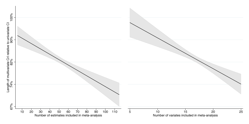
Figure 4: Mean relative lengths (with pointwise 95% confidence bands) of credible intervals provided by the multivariate model compared to univariate confidence intervals with similar coverage. Values less than 100% favor the multivariate method.

Our method provides estimates with mean bias 1.04 (95% CI 1.03 to 1.06) times higher than univariate meta-analysis. Mean absolute bias for univariate meta-analysis was estimated to be 0.02 units on the hyperbolic arctangent scale, corresponding to mean absolute bias for our method of 0.0208 (95% CI 0.0206 to 0.0212) — i.e., no additional bias to two decimal places. Our method is biased relative to the univariate method, but the magnitude of the bias may or may not be of practical importance, depending on context. Our method provides CrIs of mean length 0.84 (95% 0.82 to 0.84) times as long as CIs provided by univariate meta-analysis. In other words, our method provides credible intervals that are substantially shorter (i.e., more precise) than the univariate method, with coverage that is very close to desired 95%. There was no association between bias and total numbers of estimates or variates. This suggests that if the additional precision that our method can provide is desirable and the bias is acceptable, analysts should not be overly concerned about the number of estimates and variates available.

Figure 4 summarizes the regression results with respect to the lengths of multivariate CrIs relative to univariate CIs. We estimate that the relative length of CrIs provided by our method decreases (i.e., improves) with increasing total numbers of estimates and variates. We estimate that adding 10 estimates to a meta-analysis would result in CrIs that are on average 0.98 (95% CI 0.97 to 0.98) times as long as CIs provided by univariate meta-analysis. This may not be important in practice. However, we estimate that adding 10 variates to a meta-analysis would result in CrIs that are on average 0.87 (95% CI 0.83 to 0.92) times as long as CIs provided by univariate meta-analysis. This demonstrates that our model can make effective use of the additional information provided by additional variates and that analysts should not be overly concerned about dimensionality.

Application to knee pain data

We used our model to analyze the TKA knee pain data introduced in the motivating example above. As for that analysis, we extracted correlation coefficients or imputed them from extracted estimates of regression coefficients, risk ratios, and odds ratios. We converted correlation coefficients using Fisher’s $z$-transform (hyperbolic arctangent function) prior to meta-analysis. Further details are given in our protocol [14].

Estimation was performed as in the simulation study, with the following exceptions. We used and discarded the first 10,000 samples from each chain as burn-in and accepted the next 25,000 for a total of 100,000 posterior samples. Meta-analytical estimates were transformed back to the correlation coefficient scale using the hyperbolic tangent function. We computed surface under the cumulative ranking curve (SUCRA) values [17] to quantify the extent of evidence that the magnitude of the correlation coefficient of each predictor is greater than for all other predictors, and hence provide an indicative ranking of predictors. We summarized between-study heterogeneity using univariate $I^{2}$ statistics.

Figure 5 shows estimates of correlation coefficients between each predictor and pain measured six months post-TKA. We present posterior means and equal-tailed 95% CrIs. Note that because the systematic review is ongoing, we have disguised the names of the predictors. We compared the estimates from our model with those from White’s implementation of the model of Riley et al., and to univariate meta-analysis to assess consistency. Figure 6 shows the posterior mean variance-covariance matrix $R^{\top}\Sigma R$ (computed element-wise) estimated for the TKA knee pain data.

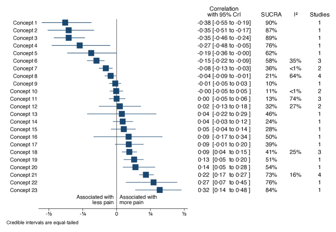
Figure 5: Forest plot showing posterior means and 95% credible intervals for the 23 predictors included in our ongoing systematic review on pain and function after total knee arthroplasty.

Discussion

We have described the problem of multivariate meta-analysis when data are sparse and proposed a tractable model that approximates within-study correlations and between-study heterogeneity in a $q$-dimensional space, where $q$ is smaller than $p$, the total number of variates of interest. The main advantages of this model are that it can be used when data are too sparse for methods proposed by Riley et al. and Lin and Chu, that it provides estimates that are on average substantially more precise compared to univariate meta-analysis (i.e., our method is statistically more powerful), and that our method provides increasingly precise estimates as the number of estimates or variates increases.

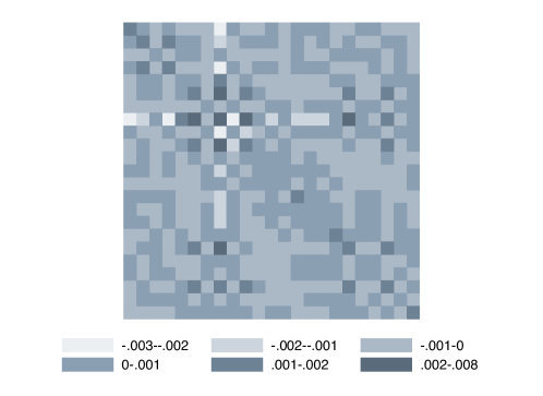
Figure 6: Posterior mean variance-covariance matrix for the total knee arthroplasty data.

We model within‐study correlation and between-study heterogeneity in a low-dimensional space via random projection. Analogously to the preservation of magnitudes and angles in orthogonal linear transforms, Johnson and Lindenstrauss showed that it is possible to embed high-dimensional data into much lower-dimensional spaces while preserving the relative distances between points [9]. Indyk et al. subsequently proposed using random matrices [12]. A wide range of distributions have been shown to yield good results with high probability [5]. While random projection is typically used in problems in which $p$ is of much higher dimension than is commonplace in multivariate meta-analysis, Lu and Lió studied random projection in low dimensions [10] and showed, perhaps unsurprisingly, that the distortion introduced when $q$ is small can be negligible if the intrinsic dimensionality of the original space is low. Our simulation study shows that our method performs well even though we use random projection in relatively low dimensions, and that precision improves as $p$ and hence $q$ increases. Random projection and related methods have subsequently become an important tool in high-dimensional statistics and machine learning, and have been applied to a range of problems, including regression [19], mixture modeling [5], text analysis [3], and medical imaging [11].

The main disadvantages of our model are that it provides estimates that are more biased compared to univariate meta-analysis (although the magnitude of the bias may not be of practical importance, depending on context), the requirement to choose $q$, and the model’s inability to disentangle the within- and between-study variances and covariances, which may be of interest in their own right. However, these disadvantages may be acceptable when $n<\frac{1}{2}p(p+3)$ and it is desirable to obtain more precise estimates than univariate meta-analysis can provide. Figure 7 suggests a decision tool that may help analysts choose an appropriate multivariate meta-analysis model. However like any rule of thumb, it should not be used unless one understands when and why one should deviate from the rule, and it does not aim to include all multivariate meta-analysis methods available.

Figure 7: Suggested approach for choosing a method to meta-analyze multivariate data.

We suggest that authors wishing to use our model report the possible limitations introduced by the low-dimensional approximation, and compare the estimates provided by our model to those from a conventional multivariate meta-analysis that includes as many variates as possible, as well as to univariate meta-analyses. Inconsistencies between models should be reported and their implications explained in a way that can be understood by non-quantitative decision-makers.

Future work could address estimating the free parameter $q$ (e.g., by placing a prior over the dimensionality of the model or otherwise integrating over $q$); using alternative dimensionality-reduction methods; modeling the distinction between studies that adjusted estimates for other variates, versus studies that did not; and modeling the scenario in which variates are not missing completely at random. Estimation in the face of sparse data remains an interesting and potentially rewarding research area.

Author contributions

CJR developed the model, performed the analyses, and wrote the manuscript. UO, MFL, EMLD, AA, and AL planned the systematic review, collected data, and contributed to the manuscript.

Funding

This work is supported by funding from the Norwegian Research Council of Norway (grant #287816) and the South-Eastern Regional Health Authority (grant #2018060).

Conflicts of interest

Within the previous five years, CJR was employed by OncoImmunity AS. He has patents and patent applications with no relevance to this study. The other authors do not report any potential conflicts of interest.

References

- [1] Beswick AD, Wylde V, Gooberman-Hill R, et al. What proportion of patients report long-term pain after total hip or knee replacement for osteoarthritis? A systematic review of prospective studies in unselected patients. BMJ Open 2012;2:e000435
- [2] Borenstein, M., Hedges, L. V., Higgins, J. P., and Rothstein, H. R. (2011). Introduction to meta-analysis. John Wiley & Sons.
- [3] Bingham, E. and Mannila, H. (2001). Random projection in dimensionality reduction: applications to image and text data. In Proceedings of the Seventh ACM SIGKDD International Conference on Knowledge Discovery and Data Mining 245-250.
- [4] Carpenter, B., Gelman, A., Hoffman, M. D., Lee, D., Goodrich, B., Betancourt, M. et al. (2017). Stan: A probabilistic programming language. Journal of Statistical Software, 76(1).
- [5] Dasgupta, S. (2000). Experiments with random projection. In Proceedings of the Sixteenth Conference on Uncertainty in Artificial Intelligence, 143-151.
- [6] Deeks, J. J. (2001). Systematic reviews of evaluations of diagnostic and screening tests. BMJ, 323(7305), 157-162.
- [7] Hoffman, M. D. and Gelman, A. (2014). The No-U-Turn sampler: adaptively setting path lengths in Hamiltonian Monte Carlo. Journal of Machine Learning Research, 15(1), 1593-1623.
- [8] Irwig, L., Macaskill, P., Glasziou, P., and Fahey, M. (1995). Meta-analytic methods for diagnostic test accuracy. Journal of Clinical Epidemiology, 48(1), 119-130.
- [9] Johnson, W. B. and Lindenstrauss, J. (1984). Extensions of Lipschitz mappings into a Hilbert space. Contemporary Mathematics, 26(189-206), 1.
- [10] Lu, Y. E., Lió, P., and Hand, S. (2008, October). On low dimensional random projections and similarity search. In Proceedings of the 17th ACM Conference on Information and Knowledge Management, 749-758.
- [11] Lustig, M., Donoho, D. L., Santos, J. M., and Pauly, J. M. (2008). Compressed sensing MRI. IEEE Signal Processing Magazine, 25(2), 72-82.
- [12] Indyk, P., and Motwani, R. (1998, May). Approximate nearest neighbors: towards removing the curse of dimensionality. In Proceedings of the Thirtieth Annual ACM Symposium on Theory of Computing, 604-613.
- [13] Lin, L. and Chu, H. (2018). Bayesian multivariate meta‐analysis of multiple factors. Research Synthesis Methods, 9(2).
- [14] Olsen, U., Lindberg, M. F., Denison, E. M. L. et al. (2020). Predictors of chronic pain and level of physical function in total knee arthroplasty: a protocol for a systematic review and meta-analysis. BMJ Open, 10(9), e037674.
- [15] Riley R.D., Thompson J.R., and Abrams K.R. (2008). An alternative model for bivariate random-effects meta-analysis when the within-study correlations are unknown. Biostatistics, 9(1).
- [16] Riley, R. D. (2009). Multivariate meta‐analysis: the effect of ignoring within‐study correlation. Journal of the Royal Statistical Society: Series A (Statistics in Society), 172(4), 789-811.
- [17] Salanti, G., A. E. Ades, and J. P. Ioannidis (2011), Graphical methods and numerical summaries for presenting results from multiple-treatment meta-analysis: an overview and tutorial. Journal of Clinical Epidemiology, 64(2), 163-71.
- [18] Tange, O. (2020). GNU Parallel 20200722 (’Privacy Shield’). Zenodo, DOI: 10.5281/zenodo.3956817
- [19] Thanei, G. A., Heinze, C., and Meinshausen, N. (2017). Random projections for large-scale regression. In Big and Complex Data Analysis, 51-68, Springer.
- [20] White IR (2009). Multivariate random-effects meta-analysis. Stata Journal; 9, 40-56.
- [21] White IR (2011). Multivariate random-effects meta-regression: Updates to mvmeta. Stata Journal; 11, 255-270.
- [22] White, I. R. (2015). Network meta-analysis. Stata Journal, 15(4), 951-985.