Assessing observability of chaotic systems using Delay Differential Analysis

Abstract

Observability can determine which recorded variables of a given system are optimal for discriminating its different states. Quantifying observability requires knowledge of the equations governing the dynamics. These equations are often unknown when experimental data are considered. Consequently, we propose an approach for numerically assessing observability using Delay Differential Analysis (DDA). Given a time series, DDA uses a delay differential equation for approximating the measured data. The lower the least squares error between the predicted and recorded data, the higher the observability. We thus rank the variables of several chaotic systems according to their corresponding least square error to assess observability. The performance of our approach is evaluated by comparison with the ranking provided by the symbolic observability coefficients as well as with two other data-based approaches using reservoir computing and singular value decomposition of the reconstructed space. We investigate the robustness of our approach against noise contamination.

A popular approach for studying nonlinear dynamical systems from a recorded time series is to reconstruct the original system using delay or derivative coordinates. It is known that the choice of the measured variable can affect the quality of attractor reconstruction. Unlike in linear systems for which the state space is observable or not from the measurements, nonlinear systems are more or less observable from measurements depending on the state space location. Moreover the observability strongly depends on the measured variables. It is therefore useful to assess the observability provided by a variable using a real number within the unit interval between two extreme values: 0 for nonobservable, and 1 for full observability. Analytical techniques for determining observability require knowledge of the underlying equations which are typically unknown when an experimental system is investigated. This is often the case for social and biological networks. It is thus of primary importance to assess observability directly from recorded time series. In this paper, we show how Delay Differential Analysis (DDA) can assess observability from time series. The performance of this approach is evaluated by comparing our results obtained for simulated chaotic systems with the symbolic observability coefficients obtained from the governing equations.

I Introduction

Studying dynamical systems from real world data can be difficult as they are often high-dimensional and nonlinear; moreover, it is typically not possible to measure all the variables spanning the associated state space.Liu, Slotine, and Barabási (2013); Wang et al. (2014); Whalen et al. (2015); Leitold, Vathy-Fogarassy, and Abonyi (2017); Haber, Molnar, and Motter (2018); Leitold, Vathy-Fogarassy, and Abonyi (2018); Letellier et al. (2018) In theory, it is possible to reconstruct the non-measured variables by using delay or differential embeddings from a single measurement.Takens (1981) However, when performing state-space reconstruction, the dimension required to obtain a diffeomorphical equivalence — required for correctly distinguishing the different states of the system — with the original state space may depend on the measured variable(s).Letellier et al. (1998) Indeed, a $d$-dimensional system can be optimally reconstructed from a given variable with a $d$-dimensional embedding but a higher-dimensional space may be required when another variable is measured. For instance, the Rössler attractor is easily reproduced with a three-dimensional global model from variable $y$ but a four-dimensional modelLetellier et al. (1998) or a quite sophisticated procedureLainscsek, Letellier, and Gorodnitsky (2003) is needed when variable $z$ is measured. It was shown that data analysis often (if not always) depends on the observability provided by the measured variable.Letellier, Aguirre, and Maquet (2006); Letellier (2006); Portes et al. (2019)

In the 1960s, the concept of observability was introduced by Rudolf Kálmán in control theory.Kalman (1959) Observability assesses whether different states of the original system can be distinguished from the measured variable. A system is said to be fully observable from some measurement if the rank of the observability matrix is equal to the dimension of the system.Kailath (1980); Chen and Ueta (1999) With such an approach, the answer is either fully observable or non observable. This approach is sufficient for linear systems because the observability matrix does not depend on the location in the state space.

This is not true for nonlinear systems and observability coefficients were introduced to overcome this inaccurate answer.Aguirre (1995); Letellier et al. (1998) Observability coefficients are real numbers within the unit interval between two extreme values, 0 for nonobservable, 1 for fully observable. These coefficients are estimated at every point of the trajectory produced by the governing equations in the state space, and then averaged along that trajectory.Aguirre (1995); Letellier et al. (1998) It is also possible to construct symbolic observability coefficients from the Jacobian matrix of the system studied.Letellier and Aguirre (2009); Bianco-Martinez, Baptista, and Letellier (2015) In this way, observability takes a graded value according to the probability with which the attractor intersects the singular observability manifold,Frunzete, Barbot, and Letellier (2012) that is, the subset of the original space for which the determinant of the observability matrix is zero. The great advantage of these coefficients is that they allow comparing the observability provided by variables from different systems and they can be computed for high-dimensional systems.Letellier et al. (2018) It is then possible to rank the variables according to the observability of the original state space they provide. The dependency of the observability on the measured variable is due to the way variables are coupled in the original system.Letellier and Aguirre (2005) Symmetries are often sources of difficulty for assessing observability, particularly because reconstructing the original symmetry is not possible from a single variable if the symmetry differs from an inversion.King and Stewart (1992); Letellier and Aguirre (2002)

The weakness of these analytical approaches is that the governing equations must be known and it is not possible to assess observability from experimental data. A first attempt to overcome this was based on a singular value decomposition of some matrices built from local data.Aguirre and Letellier (2011) Results were encouraging but some slight discrepancies with analytical results were noticed. Another approach, based on a model built directly from the data using reservoir computing was also proposed.Carroll (2018) In both cases, some discpreancies with the symbolic observability coefficients were observed. It therefore remains challenging to develop a reliable technique which always matches with theoretical results. In this work we propose a measure for assessing observability from recorded data by using delay differential analysis (DDA) and compare our results and those obtained — when available in the literature — with the two techniques discussed above with the symbolic observability coefficients computed for several well-studied chaotic systems. Here, DDA is based on a delay differential equation which approximates the dynamics underlying the measured time series. Contrary to what is done with global modelingAguirre and Letellier (2009) or reservoir computing,Pathak et al. (2017) there is no need for an accurate model. Previous work showed a rough model with a very limited number of terms (typically three) is sufficient to detect dynamical changes or classify various dynamical regime. Lainscsek et al. (2000); Lainscsek and Sejnowski (2013); Lainscsek et al. (2015)

The subsequent part of this paper is organized as follows. Section II.1 is a brief introduction to the computation of symbolic observability coefficients. Section II.2 provides an introduction to DDA and explains how it can be used for ranking variables according to the observability of the state space they provide. Section III introduces the investigated chaotic systems and provides the corresponding symbolic observability coefficients. Section IV is the main section of this paper: it discusses the performance of DDA for assessing observability of the chaotic systems and compares it with those of the two other data-based techniques. Section V provide some conclusions.

II Theoretical Background

II.1 Symbolic observability coefficients

Let us consider a $d$-dimensional dynamical system represented by the state vector $\mbox{x}\in\mbox{\bbfnt R}^{d}$ whose components are given by

$$\dot{x}_{i}=f_{i}(x_{1},x_{2},x_{3},...,x_{d}),~{}~{}~{}~{}~{}i=1,2,3,...,d$$ (1)

where $f_{i}$ is the $i$th component of the vector field f. Let us introduce the measurement function $h(\mbox{x}):\mathbb{R}^{d}\mapsto\mathbb{R}^{m}$ of $m$ variables chosen among the $d$ ones spanning the original state space. It is then required to reconstruct a space $\mathbb{R}^{d_{\rm r}}$ ($d_{\rm r}\geq d$) from the $m$ measured variables. One has to choose $d_{\rm r}-m$ derivatives of these $m$ measured variables to get a $d_{\rm r}$-dimensional vector X spanning the reconstructed space. Commonly, observability is assessed by using $d_{\rm r}=d$.Kailath (1980); Chen and Ueta (1999) In the present work, we are only working with scalar time series ($m=1$). The change of coordinate between the original state space and the reconstructed one is thus the map

$$\Phi:\mathbb{R}^{d}(\mbox{x})\mapsto\mathbb{R}^{d}(\mbox{X})\,.$$ (2)

When the derivative coordinates are used for spanning the reconstructed space, the map can be analytically computed.Letellier, Aguirre, and Maquet (2005) The observability of a system from a variable is defined as follows.Kailath (1980); Chen (1999) For the sake of simplicity, let us limit ourselves to the case $m=1$ (a generalization to the others cases is straightforward).

Definition 1

The dynamical system (1) is said to be state observable at time $t_{f}$ if every initial state $\mbox{x}(0)$ can be uniquely determined from the knowledge of the vector $s(\tau)$, $0\leq\tau\leq t_{f}$.

To test whether a system is observable or not is to construct the observability matrixHermann and Krener (1977) which is defined as the Jacobian matrix of the Lie derivatives of $h(\mbox{x})$. Differentiating $h(\mbox{x})$ yields

$$\frac{{\rm d}}{{\rm d}t}h(\mbox{x})=\frac{\partial h}{\partial\mbox{x}}\dot{\mbox{x}}=\frac{\partial h}{\partial\mbox{x}}\mbox{f}(\mbox{x})={\cal L}_{f}h(\mbox{x})\,,$$

where ${\cal L}_{f}h(\mbox{x})$ is the Lie derivative of $h(\mbox{x})$ along the vector field f. The $k$th order Lie derivative is given by

$${\cal L}_{\mbox{f}}^{k}h(\mbox{x})=\frac{\partial{\cal L}_{\mbox{f}}^{k-1}h(\mbox{x})}{\partial\mbox{x}}{\mbox{f}}(\mbox{x})\,,$$

being the zero order Lie derivative the measured variable itself, ${\cal L}_{f}^{0}h(\mbox{x})=h(\mbox{x})$. Therefore, the observability matrix ${\cal O}\in\mathbb{R}^{d\times d}$ is written as

$${\cal O}(\mbox{x})=\left[\begin{array}[]{l}{\rm d}h(\mbox{x})\\[2.84544pt] {\rm d}{\cal L}_{f}h(\mbox{x})\\[2.84544pt] \vdots\\[2.84544pt] {\rm d}{\cal L}^{d-1}_{f}h(\mbox{x})\end{array}\right]$$ (3)

where ${\rm d}\equiv\frac{\partial}{\partial\mbox{x}}$. The observability

Definition 2

The dynamical system (1) is said to be state observable if and only if the observability matrix has full rank, that is, rank$({\cal O})=d$.

The observability matrix ${\cal O}$ is equal to the Jacobian matrix of the change of coordinates $\Phi:\mbox{x}\rightarrow\mbox{X}$ when derivative coordinates are used.Letellier, Aguirre, and Maquet (2005) In this approach, the observability is either full or zero. The term structural was introduced when the results do not depend on parameter valuesLin (1974). Computing the rank of the observability matrix is independent of parameter values and, consequently, is an example of structural observability.Aguirre, Portes, and Letellier (2018) Computing observability with graphsLin (1974); Liu, Slotine, and Barabási (2013); Letellier, Sendiña-Nadal, and Aguirre (2018) is also a structural approach. We term observability assessed from recorded data — necessarily dependent on the parameter values used for simulating the trajectory of the system —as dynamical observability.Aguirre, Portes, and Letellier (2018) This type of approach returns a real number within the unit interval: variables can be ranked between the two extreme cases, 1.0 (0.0) for a full (null) observability There is a third type of observability, symbolic observability, which does not depend on parameter values but allows ranking the variables.Bianco-Martinez, Baptista, and Letellier (2015) All types of observability are not sensitive to symmetry-related problems. This is due to the fact that observability is a local property while symmetry is a global one. Consequently, symmetry may degrade the assessment of observability.Letellier and Aguirre (2002)

The procedure to compute symbolic observability coefficients is implemented in three steps as follows.Bianco-Martinez, Baptista, and Letellier (2015); Letellier et al. (2018) First, the Jacobian matrix ${\cal J}$ of the system (1), composed of elements $J_{ij}$, is transformed into the symbolic Jacobian matrix $\tilde{\cal J}$ by replacing each constant element $J_{ij}$ by 1, each polynomial element $J_{ij}$ by $\bar{1}$, and each rational element $J_{ij}$ by $\bar{\bar{1}}$ when the $j$th variable is present in the denominator, or by $\bar{1}$ otherwise. Rational terms in the governing equations (1) are distinguished from polynomial terms since the formers reduce more strongly the observability than the latters.Bianco-Martinez, Baptista, and Letellier (2015)

Then the symbolic observability matrix $\tilde{\cal O}$ is constructed. The first row of $\tilde{\cal O}$ is defined by the derivative of the measurement function ${\rm d}h(\mbox{x})$, that is, $\tilde{O}_{1j}=1$ if $j=i$ and $0$ otherwise when the $i$th variable is measured. The second row is the $i$th row of $\tilde{\cal J}$. The $k$th row is obtained as follows. First, each element of the $i$th row of $\tilde{\cal J}$ is multiplied by the corresponding $i$th component of the vector $\mbox{v}=(\tilde{O}_{\ell 1},\cdots,\tilde{O}_{\ell d})^{\rm T}$ where $\ell=k-1$ refers to the $(k-1)$th row of the symbolic observability matrix $\tilde{\cal O}$. The rules to perform the symbolic product $\tilde{J}_{ij}\otimes v_{i}$ are such that Bianco-Martinez, Baptista, and Letellier (2015)

$$\left|\begin{array}[]{ll}0\otimes a&=0,\\[2.84544pt] 1\otimes a&=a,\\[2.84544pt] \bar{1}\otimes a&=a\text{ for }a=\bar{1},\bar{\bar{1}},\\[2.84544pt] \bar{\bar{1}}\otimes a&=\bar{\bar{1}}\text{ for }a\neq 0.\end{array}\right.$$ (4)

Second, the matrix $\tilde{\cal J}^{\prime}$ is reduced into a row where each element $\tilde{O}_{kj}=\sum_{i}\tilde{J}^{\prime}_{ij}$ according to the addition lawBianco-Martinez, Baptista, and Letellier (2015)

$$\left|\begin{array}[]{ll}0\oplus a&=a,\\[2.84544pt] 1\oplus a&=a\text{ for }a\neq 0,\\[2.84544pt] \bar{1}\oplus a&=a\text{ for }a\neq 0,1,\\[2.84544pt] \bar{\bar{1}}\oplus a&=\bar{\bar{1}}.\end{array}\right.$$ (5)

The last step is associated with the computation of the symbolic observability coefficients. The determinant of $\tilde{\cal O}$ is computed according to the symbolic product rule defined in (4) and expressed as products and addends of the symbolic terms $1$, $\bar{1}$ and $\bar{\bar{1}}$, whose number of occurrences are $N_{1}$, $N_{\bar{1}}$ and $N_{\bar{\bar{1}}}$, respectively. It is convenient to impose that, if $N_{\bar{1}}=0$ and $N_{\bar{\bar{1}}}\neq 0$ then $N_{\bar{1}}=N_{\bar{\bar{1}}}$. The symbolic observability coefficient is thus defined as

$$\eta=\displaystyle\frac{1}{D}{N_{1}}+\frac{1}{D^{2}}N_{\bar{1}}+\frac{1}{D^{3}}N_{\bar{\bar{1}}}$$ (6)

with $D=N_{1}+N_{\bar{1}}+N_{\bar{\bar{1}}}$. This coefficient is in the unit interval, $\eta=1$ for a variable providing full observability of the original state space. An observability is said to be good when $\eta\geq 0.75$.Sendiña-Nadal, Boccaletti, and Letellier (2016)

II.2 Delay Differential Analysis

Let us assume that a time series $\left\{X_{1}\right\}$ is recorded in a $d$-dimensional system. From this time series, it is possible to obtain a global model reproducing the underlying dynamics. There are typically two main approaches working with either derivative or delay coordinates.Crutchfield and McNamara (1987); Aguirre and Letellier (2009) When derivatives are used, it is possible to construct a $d$-dimensional differential model

$$\left\{\begin{array}[]{l}\dot{X}_{1}=X_{2}\\[2.84544pt] \dot{X}_{2}=X_{3}\\[2.84544pt] \vdots\\ \dot{X}_{d}=F\left(\displaystyle X_{1},X_{2},...,X_{d}\right)\end{array}\right.$$ (7)

where $X_{i}$ is the $(i-1)$th derivative of the measured variable $X_{1}$.Gouesbet and Letellier (1994) The function $F$ can be numerically estimated by using a least-square technique with a structure selection.Mangiarotti et al. (2012); Mangiarotti and Huc (2019) $F$ can be polynomialGouesbet and Letellier (1994); Mangiarotti and Huc (2019) or rational.Lainscsek, Letellier, and Schürrer (2001); Lainscsek (2011) This model requires $d$-ordinary differential equations whose variables are the $d$ successive derivatives of $X_{1}$: this model works in a differentiable embedding.

Second, it is possible to construct a model whose equations have the form of a difference equation

$$X(k+1)=F\left(\displaystyle X_{\tau_{j}}(k)\right)=\sum_{i=0}^{N}{\displaystyle a_{i}\,\varphi_{i}}$$ (8)

where $\varphi_{i}$ is a monomial of delay coordinates $X_{\tau_{j}}(k)=X(k-\tau_{j})$ with $\tau_{j}=n\delta_{t}$ ($n\in\mathbb{N}^{+}$) is a time delay expressed in terms of the sampling time $\delta_{t}$ with which the scalar time series $\{X_{1}(k)\}$ is recorded: $k$ is the discrete time. Such a model has an auto-regressive form, and typically the number $N$ of terms is between 10 and 20. The space in which this model is working is thus spanned by delay coordinates: its dimension is very often significantly larger than the dimension $d$, the embedding dimensionCao (1997) or even than the Takens criterion.Takens (1981) An optimal form of the difference equation (8) is developed under the form of a nonlinear autoregressive-moving average (NARMA) model.Aguirre and Billings (1995a)

Recently a third type of model was investigated under the name of reservoir computing.Lukosevicius and Jaeger (2009) This approach considers an oversized model with a functional structure based on a network whose nodes are characterized by some simple function. For instance, the Lorenz attractor was accurately reproduced with a Erdös-Rényi network of 300 nodes with a mean degree $\overline{\delta}=6$, each node being made of a difference equation.Pathak et al. (2017) The model so-obtained corresponds to an accurate global model of the dynamics. Notably, this model was constructed from the measurements of all the variables of the Lorenz system. The main advantage of such a large model is its flexibility, that is, its ability to capture various dynamical regimes, but it has the disadvantage that the space in which it is working is not clearly defined and has a very large dimension ($d_{\rm r}>300$ in the work discussed above).

The DDA approach uses a kind of mixed model between the differential model (7) and the difference equation (8), the left member of the latter being replaced with the left member of the former. It is therefore based on the delay differential equation

$$\dot{X}=\mathcal{F}_{X}=\sum\limits_{i=1}^{N}{\displaystyle a_{i}\,\varphi_{i}(X_{\tau_{j}})}\,$$ (9)

where $X=X_{1}$ designates the measured variable and $X_{\tau_{j}}$ some delay coordinates. The purpose is not to construct a global model reproducing accurately the dynamics but only an approximated model for detecting dynamical changes (nonstationarity) or classifying different dynamical regimes.Lainscsek et al. (2000); Lainscsek and Sejnowski (2013); Lainscsek et al. (2017) We therefore use a rough model with very few terms ($N\leq 3$). Such sparsity in the model prevents overparametrization, that is, spurious dynamics induced by overly complex models.Aguirre and Billings (1995b) Indeed, delay differential equations are known to already produce complex dynamics with only two terms.Mackey and Glass (1977); Farmer (1982) Many characteristics of the measured dynamics can be captured with two or three terms and appropriate time delays.Lainscsek et al. (2015) Based on previous works,Lainscsek et al. (2000); Lainscsek and Sejnowski (2013); Lainscsek et al. (2015, 2017) it is assumed that these characteristics are sufficient to distinguish different dynamical regimes. This DDA model (9) is a differential equation whose state space is spanned by delay coordinates $X_{\tau_{j}}$.

Model (9) has two sets of parameters, the fixed parameters $\tau_{j}$ (set during the structure selection) and the free parameters $a_{i}$ (estimated independently from each data window). The structure of model (9) as well as the delays are determined for each time series. Then, the free coefficients $a_{i}$ are determined for each window of the recorded time series. The data in each window$\left\{X_{1}\right\}$ is normalized to have zero mean and unit variance to remove amplitude information before estimating the free parameters $a_{i}$ by using a singular value decomposition (SVD). The least-square error

$$\rho_{X}=\sqrt{\frac{1}{K}\sum_{k=1}^{K}\displaystyle\left(\displaystyle\dot{X}(k)-\mathcal{F}_{X}(k)\right)^{2}}\,$$ (10)

between the derivatives returned by the DDA model and the derivatives computed from the measured time series quantifies the ability of the model to capture the underlying dynamics. It is known that there is a relationship between the model quality and observability.Letellier et al. (1998); Letellier and Aguirre (2002); Letellier, Aguirre, and Maquet (2006) The signal derivative $\dot{X}_{1}$ is computed using a five-point center derivative.Miletics and Molnárka (2004) In this work, structure selection (i.e. choosing the model form of Eq. (9) and the fixed parameters $\tau_{j}$) was performed via an exhaustive search over all possible three-term models (three monomials: $N=3$) with two delays such that $\tau_{j}\in[m+1;60]\delta_{t}$, where $m=5$ is equal to the number of points for estimating the derivative and $\delta_{t}$ is the sampling time. Function $\mathcal{F}$ is made of three monomials selected from the possible candidates

$$\begin{array}[]{rl}\varphi_{i}\in&\left\{\displaystyle X_{\tau_{1}},X_{\tau_{2}},X_{\tau_{1}}^{2},X_{\tau_{1}}\,X_{\tau_{2}},X_{\tau_{2}}^{2},\right.\\[2.84544pt] &\left.\displaystyle~{}~{}~{}~{}~{}~{}~{}~{}~{}X_{\tau_{1}}^{3},X_{\tau_{1}}^{2}\,X_{\tau_{2}},X_{\tau_{1}}\,X_{\tau_{2}}^{2},X_{\tau_{2}}^{3}\right\}\,.\end{array}$$ (11)

Monomials and delays are selected in an exhaustive search over all possible model forms, i.e. 44, and delay combinations under the restrictions specified above. Each model is thus characterized by the set of “fixed” parameters $(\tau_{1},\tau_{2})$, the corresponding monomials $\varphi_{i}$, and the free parameters $a_{i}$ which are estimated for each time window of the measuredndata. The structure providing the model with the lowest $\rho_{X}$ is retained to assess observability according to the model error $\rho_{X}$.

As used with reservoir computing,Carroll (2018) the error $\rho_{X}$ between the model and the measured data provides a measure of how the system dynamics may be reconstructed from these data. Indeed, to obtain a reliable deterministic model, it is necessary to distinguish every different state of the system for retrieving the underlying causality. Since the error is used as a relative measure, it is only needed to have a sufficiently flexible functional form for the model as observed with reservoir computing or with a delay differential equation. Consequently the smaller the error $\rho_{X}$, the higher the observability provided by the variable $X$. This results from previous works where it was shown that the complexity of the model to approximate was correlated to the observability: the better the observability provided by the measured variable, the simpler the model to approximate.Letellier and Aguirre (2002); Letellier, Aguirre, and Maquet (2006) The error $\rho_{X}$ from the best DDA model is computed with an increasing noise amplitude. For each three-dimensional system and each signal-to-noise ratio (no noise, 20, 10 and 0 dB: where 0dB indicates the variance of the noise matches the variance of the signal), the error $\rho_{X}$ was computed over several hundred pseudoperiods for each time series.

III Dynamical systems and observability coefficients

III.1 Low-dimensional systems

The governing equations of the systems here investigated are reported in Table 1. The symbolic observability coefficients (SOC) and the model error $\rho_{X}$ are reported for each variable of every system in Table 1. Parameter values are reported in Table 2.

Table 1: Governing equations of each system for which the symbolic observability coefficients (SOC) $\eta_{s^{3}}$ and $\rho_{X}$ between the DDA model and the measured data with no noise contamination are reported. The SOC for variable $x$ of the Hindmarsh-Rose (HR) system is corrected as discussed in the main text.For the Chua system, $f(x)=bx+\frac{1}{2}(a-b)(|x+1|-|x-1|)$

System	Equations	SOC	Error
Rössler 76	$\dot{x}=-y-z$	$0.84$	0.037
Rössler (1976)	$\dot{y}=x+ay$	1.0	0.022
	$\dot{z}=b+z(x-c)$	$0.56$	0.106
Rössler 77	$\dot{x}=-ax-y(1-x^{2})$	0.56	$0.0009$
Rössler (1977)	$\dot{y}=\mu(bx+y-cz)$	0.84	$0.0005$
	$\dot{z}=\mu(x+cy-dz)$	0.68	$0.0007$
Lorenz 63	$\dot{x}=\sigma(y-x)$	0.78	0.02
Lorenz (1963)	$\dot{y}=Rx-y-xz$	0.36	0.039
	$\dot{z}=-bz+xy$	0.36	0.071
Lorenz 84	$\dot{x}=-y^{2}-z^{2}-ax+aF$	0.36	0.061
Lorenz (1984)	$\dot{y}=xy-bxz-y+G$	0.36	0.205
	$\dot{z}=bxy+xz-z$	0.36	0.204
Cord	$\dot{x}=-y-z-ax+aF$	0.68	0.108
Letellier and Aguirre (2012)	$\dot{y}=xy-bxz-y+G$	0.36	0.198
	$\dot{z}=bxy+xz-z$	0.36	0.232
HR	$\dot{x}=y-ax^{3}+bx^{2}+I-z$	0.68	0.025
Hindmarsh and Rose (1984)	$\dot{y}=c-dx^{2}-y$	0.56	0.023
	$\dot{z}=r[s(x-x_{\rm R})-z]$	1.00	0.002
Fisher	$\dot{x}=y$	1.00	0.003
Fischer et al. (1999)	$\dot{y}=-ax-by-z$	0.84	0.004
	$\dot{z}=b+x-|x|$	0.56	0.027
Chua	$\dot{x}=\alpha(-x+y-f(x))$	1.00	0.05
Chua, Yao, and Yang (1986)	$\dot{y}=x-y+z$	0.84	0.068
	$\dot{z}=-\beta y$	1.00	0.066
Duffing	$\dot{x}=y$	1.00	0.022
Duffing (1918); Ménard et al. (2000)	$\dot{y}=-\mu y+x-x^{3}+u$	0.86	0.08
	$\dot{u}=v$	0.00	0.00
	$\dot{v}=-\omega^{2}u$	0.00	0.00
Rössler 79	$\dot{x}=-y-z$	0.75	0.005
Rössler (1979)	$\dot{y}=x+ay+w$	0.83	0.001
	$\dot{z}=b+xz$	0.44	0.079
	$\dot{w}=-cz+dw$	0.63	0.006
Hénon-Heiles	$\dot{x}=u$	0.64	0.0005
Hénon and Heiles (1964)	$\dot{y}=v$	0.64	0.0004
	$\dot{u}=-x-2xy$	0.44	0.0009
	$\dot{v}=-y-y^{2}-x^{2}$	0.44	0.0008

The Rössler 76Rössler (1976), Lorenz 84Lorenz (1984), CordLetellier and Aguirre (2012), Hindmarsh-RoseHindmarsh and Rose (1984) (HR) and FisherFischer et al. (1999) systems have no symmetry. The Hindmarsh-Rose system is known to be problematic when variable $x$ or $z$ is measured, for two different reasons.Aguirre, Portes, and Letellier (2017) When variable $z$ is measured, the observability matrix

$${\cal O}_{z}=\left[\begin{array}[]{ccc}0&0&1\\[2.84544pt] rs&0&-r\\[2.84544pt] rs\left(\displaystyle x\chi-r\right)&rs&r(r-s)\end{array}\right]$$ (12)

where $\chi=2b-3ax$ becomes singular when $r$ is too small (Det${\cal O}_{z}=r^{2}s^{2}$): the observability can be null for $r=0$ and full for $r\neq 0$ (this is also true for $s$, but $s$ is commonly significantly different from 0). When variable $x$ is measured, although the observability matrix ${\cal O}_{x}$ is never singular (Det ${\cal O}_{x}=r-1$), the plane projection of the differential embedding induced by variable $x$ does not reveal the chaotic nature of the underlying dynamics, contrary to what is clearly provided by variable $z$ (Fig. 1). As discussed by Aguirre et al,Aguirre, Portes, and Letellier (2017) the observability matrix

$${\cal O}_{x}=\left[\begin{array}[]{ccc}1&0&0\\[2.84544pt] \chi x&1&1\\[2.84544pt] O_{31}^{x}&\chi x-1&-\chi x+r\end{array}\right]$$ (13)

where

$$\begin{array}[]{rl}O_{31}^{x}=&\displaystyle\chi^{2}x^{2}-rs-2bx+2(b-3a)\\ &~{}~{}~{}\times\left[\left(\displaystyle I+x^{2}(b-ax)+y-z\right)\right]\end{array}$$ (14)

has a determinant Det ${\cal O}_{x}$ whose polynomial nature is cancelled by the contributions of $O_{32}$ and $O_{33}$ but this is not structurally stable. Any perturbation in one of these two elements would lead to a determinant vanishing for a subset of the state space. This is not detected by the symbolic observability coefficients. If we keep the polynomial nature of elements $O_{32}$ and $O_{33}$, the symbolic observability matrix would be

$${\cal O}_{x}=\left[\begin{array}[]{ccc}1&0&0\\[2.84544pt] \bar{1}&1&1\\[2.84544pt] \bar{1}&\bar{1}&\bar{1}\end{array}\right]\,.$$ (15)

The corresponding corrected symbolic observability coefficient is thus $\eta^{\prime}_{x^{3}}=0.68$. The corrected ranking of variables is therefore $z\vartriangleright x\vartriangleright y$. This ranking will be used in the subsequent analysis.

Table 2: Parameter values of the investigated systems.

Rössler 76	$a=0.52$	$b=2$	$c=4$
Rössler 77	$a=0.03$	$b=0.3$	$c=2$	$d=0.5$
	$\mu=0.1$
Lorenz 63	$\sigma=10$	$b=8/3$	$R=28$
Lorenz 84	$a=0.28$	$b=4$	$F=8$	$G=1$
Cord	$a=0.28$	$b=4$	$F=8$	$G=1$
HR	$a=1$	$b=3$	$c=1$	$d=5$
	$I=3.29$	$x_{\rm R}=\frac{8}{5}$
Fisher	$a=0.3$	$b=0.097$
Chua	$\alpha=9$	$\beta=\frac{100}{7}$	$a=-\frac{8}{7}$
	$b=-\frac{5}{7}$
Duffing	$\mu=0.3$	$\omega=1.2$
	$x_{0}=1$	$y_{0}=0$	$u_{0}=0.5$	$v_{0}=0$
Rössler 79	$a=0.25$	$b=3$	$c=0.5$	$d=0.05$

Figure 1: Differential embedding induced by each of the three variables of the Hindmarsh-Rose system.

The other systems have symmetry properties as follows. The Lorenz 63 systemLorenz (1963) is equivariant under a ${\cal R}_{z}$ rotation symmetry around the $z$-axis.Letellier, Dutertre, and Gouesbet (1994); Letellier and Gilmore (2001) Variables $x$ and $y$ are mapped into their opposite ($-x$ and $-y$, respectively) while variable $z$ is invariant under the rotation symmetry. At least two variables must be measured to correctly reconstruct the rotation symmetry.King and Stewart (1992) The Rössler 77Rössler (1977) , Chua circuitChua, Yao, and Yang (1986) and the driven Duffing systemsDuffing (1918); Ménard et al. (2000) are equivariant under an inversion symmetry. Such a symmetry can be recovered from a single variable and, consequently, should not blur the observability analysis. The driven Duffing system is in fact a four-dimensional system, a conservative harmonic oscillator driving the dissipative Duffing oscillator: it is thus a semi-dissipative (or semi-conservative) system.Ménard et al. (2000) When variable $u$ (or $v$) is recorded , a periodic orbit is obtained while variable $x$ (or $y$) provides a chaotic state portrait. Since a chaotic driving signal necessarily implies a chaotic response, it is obvious that $u$ drives $x$ and not the opposite. It can therefore be concluded, without further analysis, that the system is not observable from $u$ (or $v$). Thus, we only have to determine the observability from variable $x$ and $y$, respectively. The Fisher system and the Chua circuit have a piecewise nonlinearity. They will be useful to test whether DDA is robust against discontinuous nonlinearity.

All these systems but three — the Lorenz 84, the Cord, and the Hénon-HeilesHénon and Heiles (1964) systems — have at least one variable providing a good observability ($\eta>0.75$) of the original state space. The Hénon-Heiles system is conservative and one may guess that the observability problem will be more sensitive since the invariant domain of the state space has a dimension close to 3, and not 2 as for all the other systems which are strongly dissipative.

III.2 A higher-dimensional system

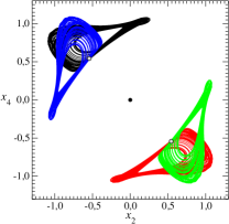
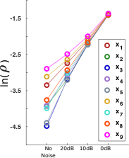
(a)
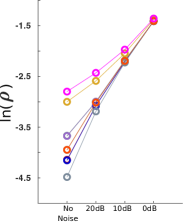
(b)
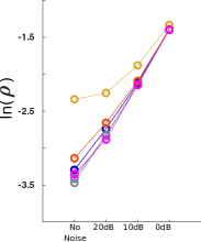
(c)
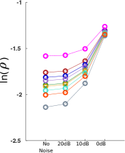
(d)

Figure 2: Chaotic attractor produced by the 9D Lorenz system (18). (a) $R=14.22$, (b) $R=14.30$, (c) $R=15.10$, (d) $R=45.00$. Other parameter values: $a=0.5$, and $\sigma=0.5$. When there are co-existing attractors, they are plotted in different colors in the plane projections of the state space.

The Lorenz 63 system results from a Galerkin expansion of the Navier-Stokes equations for Rayleigh-Bénard convection.Saltzman (1962) It is also possible to have a higher-dimensional expansion in retaining more Fourier components. One of them lead to the 9D Lorenz systemReiterer et al. (1998)

$$\left\{\begin{array}[]{l}\dot{x_{1}}=-\sigma(b_{1}x_{1}+b_{2}x_{7})+x_{4}(b_{4}x_{4}-x_{2})+b_{3}x_{3}x_{5}\\[2.84544pt] \displaystyle\dot{x_{2}}=-\sigma{x_{2}}+x_{1}x_{4}-x_{2}x_{5}+x_{4}x_{5}-\frac{\sigma x_{9}}{2}\\[2.84544pt] \dot{x_{3}}=\sigma(b_{2}x_{8}-b_{1}x_{3})+x_{2}x_{4}-b_{4}{x_{2}^{2}}-b_{3}{x_{1}x_{5}}\\[2.84544pt] \displaystyle\dot{x_{4}}=-\sigma{x_{4}}-x_{2}x_{3}-x_{2}x_{5}+x_{4}x_{5}+\frac{\sigma x_{9}}{2}\\[2.84544pt] \displaystyle\dot{x_{5}}=-\sigma{b_{5}}x_{5}+\frac{x_{2}^{2}}{2}-\frac{x_{4}^{2}}{2}\\[2.84544pt] \dot{x_{6}}=-b_{6}x_{6}+x_{2}x_{9}-x_{4}x_{9}\\[2.84544pt] \dot{x_{7}}=-b_{1}{x_{7}}-Rx_{1}+2x_{5}x_{8}-x_{4}x_{9}\\[2.84544pt] \dot{x_{8}}=-b_{1}{x_{8}}+Rx_{3}-2x_{5}x_{7}+x_{2}x_{9}\\[2.84544pt] \dot{x_{9}}=-x_{9}+(R+2x_{6})(x_{4}-x_{2})+x_{4}x_{7}-x_{2}x_{8}\end{array}\right.$$ (16)

where

$$\left\{\begin{array}[]{ll}\displaystyle b_{1}=4\frac{1+a^{2}}{1+2a^{2}}&\displaystyle b_{2}=\frac{1+2a^{2}}{2(1+a^{2})}\\[8.5359pt] \displaystyle b_{3}=2\frac{1-a^{2}}{1+a^{2}}&\displaystyle b_{4}=\frac{a^{2}}{1+a^{2}}\\[8.5359pt] \displaystyle b_{5}=\frac{8a^{2}}{1+2a^{2}}&\displaystyle b_{6}=\frac{4}{1+2a^{2}}\end{array}\right.$$ (17)

This 9D Lorenz system is equivariant.Gilmore and Letellier (2007) Depending on the $R$-values, the attractor produced may be asymmetric [Fig. 2(a)] or symmetric [Fig. 2(b)]. The symbolic observability coefficients are

$$\left\{\begin{array}[]{l}\displaystyle\eta_{x_{1}^{9}}=\eta_{x_{3}^{9}}=\eta_{x_{7}^{9}}=\eta_{x_{8}^{9}}=0.04\\[2.84544pt] \displaystyle\eta_{x_{2}^{9}}=\eta_{x_{4}^{9}}=0.03\\[2.84544pt] \displaystyle\eta_{x_{5}^{9}}=\eta_{x_{6}^{9}}=\eta_{x_{9}^{9}}=0\end{array}\right.$$ (18)

leading to

$$x_{1}=x_{3}=x_{7}=x_{8}\vartriangleright x_{2}=x_{4}\vartriangleright x_{5}=x_{6}=x_{9}$$

Notice that every variable offers an extremely poor observability of the original state space. It was shown that, at least five variables need to be measured for having a good observability ($\eta>0.75$) of the original state space.Letellier et al. (2018) Moreover, for a sufficiently large $R$-value ($R=45$), the behavior is hyperchaotic. One of the characteristics of this highly developed behavior is that there are two different time scales. We will therefore investigate whether the observability assessed with DDA is dependent on parameter values, that is, on bifurcation affecting the symmetry properties (order-4 or order-2 asymmetric chaos, symmetric chaos and hyperchaos).

IV DDA ranking

The structure of the best DDA models ${\cal F}_{X}$ are reported in Appendix A, Table 5 along with the corresponding time delays retained for identifying the free parameters. As examples, $\rho_{X}$ for some systems with increasing noise are shown in Figs. 3. For no noise, $\rho_{X}$ is reported in Table 1.

The rankings for variables according to increasing symbolic observability coefficients (SOC), decreasing $\rho_{X}$ for DDA, and when available in the literature, for decreasing reservoir computing (RC) and singular value decomposition observability (SVDO) are summarized in Table 3 for all low dimensional systems ($d\leq 4$). The results for the Rössler 76, Rössler 77, Fisher, driven Duffing and Rössler 79Rössler (1979) systems are in a perfect agreement with the SOC. The discontinuity of the Fisher system does not perturb the analysis. The hyperchaotic nature of the Rössler 79 system was not problematic for correctly assessing observability.

The Lorenz 63, Lorenz 84, Cord and Hindmarsh-Rose systems show close agreement between DDA and SOC. For the Lorenz 63 system, variable $x$ was correctly detected as providing the best observability but variable $z$ was found to offer worse observability than variable $y$, a feature which is not predicted by the SOC due to a problem inherent to the symmetry involved. For the Cord system, while no single variable provides good observability for the original state space, DDA correctly ranks $x$ as providing the best observability. However, DDA ranks $z$ as providing worse observability than variable $y$, while SOC ranks them with equivalent observability. For the Hindmarsh-Rose system, variable $z$ provides full observability and is associated with the lowest $\rho_{X}$. However, there is some discrepancy between DDA and SOC since, as assessed with DDA, $y$ provides a slightly higher observability than $x$. Results for the Hénon-Heiles system are quite equivalent to the SOC.Variables $x$ and $y$ are more observable than $u$ and $v$, however, $x$($u$) is more observable than $y$($v$) instead of showing equivalent observability.

For the Chua circuit, the variable $x$ contains a piecewise nonlinearity and has full observability, and DDA correctly ranks $x$ as the most observable. DDA also ranks variable $y$ with the worst observability, which is in agreement with SOC. However, variable $z$ has only slightly better observability than $y$, whereas it should be equivalent to $x$.

Table 3: Ranking variables according to the observability as assessed by the symbolic observability coefficients (SOC), DDA analysis, reservoir computing (RC) and singular value decomposition observability (SVDO). A perfect agreement with the SOC is indicated by a $\bullet$. When the variable providing the best observability is correctly detected or when $=$ is replaced with $\thickapprox$ or $\vartriangleright$, a $\circ$ is reported.

System	SOC	DDA	RC	SVDO
Rössler 76	$y\vartriangleright x\vartriangleright z$	$\bullet$	$x\vartriangleright y\vartriangleright z$	$\bullet$
Rössler 77	$y\vartriangleright z\vartriangleright x$	$\bullet$	—	—
Lorenz 63	$x\vartriangleright y=z$	$\circ$	$y\vartriangleright x\vartriangleright z$	$\circ$
Lorenz 84	$x=y=z$	$\circ$	—	$\bullet$
Cord	$x\vartriangleright y=z$	$\circ$	—	$\circ$
Hindmarsh-Rose	$z\vartriangleright x\vartriangleright y$	$\circ$	—	$\bullet$
Fisher	$x\vartriangleright y\vartriangleright z$	$\bullet$	—	—
Chua	$x=z\vartriangleright y$	$\circ$	$\bullet$	$\circ$
Duffing	$x\vartriangleright y\vartriangleright u=v$	$\bullet$	—	—
Rössler 79	$y\vartriangleright x\vartriangleright w\vartriangleright z$	$\bullet$	$x\vartriangleright y\vartriangleright z\vartriangleright w$	$x\vartriangleright y\vartriangleright w\vartriangleright z$
Hénon-Heiles	$x=y\vartriangleright u=v$	$\circ$	$\circ$	—

When compared to the two other data-based techniques, DDA performs better than RC for the Rössler 76, Rössler 79 and the Lorenz 63 systems but not for the Chua circuit. Compared to the SVDO, the DDA approach provides equivalent results for all the systems investigated by these two techniques, but does perform better for the hyperchaotic Rössler 79 system in correctly identifying the variable $y$ as providing the best observability, a feature which missed by the SVDO.

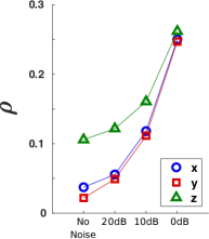
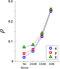
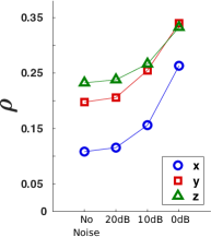
(a)		(b)		(c)
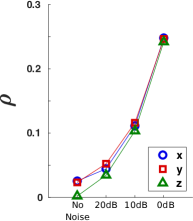
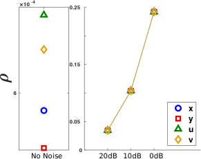
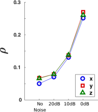
(d)		(e)		(f)

Figure 3: Error $\rho_{X}$ versus a decreasing signal-to-noise ratio for some of the different systems investigated in this paper. (a) Rössler 76 system, (b) Lorenz 63 system, (c) Cord system, (d) Hindmarsh-Rose system, (e) Hénon-Heiles system, (f) Chua system.

For most of the systems, these results are robust against noise contamination, at least up to a signal-to-noise ratio greater than 10 dB: below this ratio, results can be blurred and observability can no longer be reliably assessed using DDA. A similar robustness was observed with SVDO. It was not investigated with RC.

Note that another interesting data-based technique for assessing observability was proposed by Parlitz and co-workers.Parlitz, Schumann-Bischoff, and Luther (2014) It was only tested with the Rössler 76 system (and the Hénon map, not investigated here). It would be interesting to further investigate its performance but this is out of the scope of this paper.

The results for the 9D Lorenz system are not so clear. The first reason is that this system is nearly unobservable from a single variable. The SOC are nearly saturated (close to 0) with nonlinear elements as revealed by the symbolic Jacobian matrix of the 9D Lorenz system (16), namely

$${\cal J}^{\rm sym}=\left[\begin{matrix}1&\bar{1}&\bar{1}&\bar{1}&\bar{1}&0&1&0&0\\ \bar{1}&\bar{1}&0&\bar{1}&\bar{1}&0&0&0&1\\ \bar{1}&\bar{1}&1&\bar{1}&\bar{1}&0&0&1&0\\ 0&\bar{1}&\bar{1}&\bar{1}&\bar{1}&0&0&0&1\\ 0&\bar{1}&0&\bar{1}&\bar{1}&0&0&0&0\\ 0&\bar{1}&0&\bar{1}&0&1&0&0&\bar{1}\\ 1&0&0&\bar{1}&\bar{1}&0&1&\bar{1}&\bar{1}\\ 0&\bar{1}&1&0&\bar{1}&0&\bar{1}&1&0\\ 0&\bar{1}&\bar{1}&0&\bar{1}&\bar{1}&\bar{1}&\bar{1}&1\\ \end{matrix}\right]\,,$$ (19)

which illustrates most of the couplings between variables are nonlinear. Considering only the observability provided by a single variable is here investigated, and that the SOC are all close to 0, one may conclude that the 9D Lorenz system is not observable from a single variable.

Results provided by DDA are shown in Fig. 2 where it is seen that variables cannot be easily ranked, particularly when $R$ is increased. Results are summarized in Table 4 as follows. For each $R$-values, the rankings of the variables are reported — from 1 for the variable offering the best observability to 9 for the one providing the poorest observability — and compared to the ranking provided by the SOC. The results are strongly dependent on $R$-value in a way which does not allow to extract a clear tendency. Variable $x_{5}$ with a null observability as assessed by the SOC (and analytically) is found to provide the best observability as assessed by DDA. Nevertheless, this is in agreement with the successful three-dimensional global model obtained from this variable for $R=14.22$,Reiterer et al. (1998) that is, at least for this $R$-value, the dynamics can be correctly reconstructed for recovering the underlying determinism.

Table 4: Observability of the 9D Lorenz system as assessed with the symbolic observability coefficients (SOC) and DDA.

	$R$	$x_{1}$	$x_{2}$	$x_{3}$	$x_{4}$	$x_{5}$	$x_{6}$	$x_{7}$	$x_{8}$	$x_{9}$
SOC	—	1	2	1	2	3	3	1	1	3
DDA	14.22	7	4	1	5	2	8	3	6	9
	14.30	3	7	2	6	1	8	5	4	9
	15.10	5	2	6	3	1	9	8	7	4
	45.00	8	5	7	6	1	4	3	2	9

It should be pointed out that looking for full observability (i.e. being able to “reconstruct” each of the non-measured variables) is not the same thing as looking for an embedding. Especially for large $d$-dimensional systems producing an attractor which can be embedded within a space whose dimension $d_{\rm R}$ is lower than the dimension $d$ of the original state space. Full observability ensures the existence of an embedding, the opposite is not necessarily true. Here DDA selects the variable which provides the best reconstructed space. If compared with the results provided by the SOC with multivariate measurements,Letellier et al. (2018) variables $x_{2}$, $x_{4}$, $x_{5}$, and $x_{6}$ are always among the six variables selected for providing a full observability. DDA returns three of them as providing the best observability, $x_{2}$, $x_{4}$, and $x_{5}$ (Table 4). Variable $x_{6}$, the single one which is invariant under the symmetry of this system, is identified as a variable providing a poor observability. Once again, symmetry induces difficulties for assessing observability.

V Conclusion

The ability to infer the state of a system from a scalar output depends on which system variable is measured. We have introduced a numerical approach using the error between a DDA model and measured data to assess the observability provided by the measured variables in several chaotic systems. We compared these measures with symbolic observability coefficients, which are determined directly from the system’s equations. Our measure overall reliably ranks variables according to the observability they provide about the original state space. The largest discrepancy was obtained for a large-dimensional (9D Lorenz) system. The smaller the model error, the better the observability provided. The assessment of observability is quite robust against noise contamination in the majority of the systems here considered.

There are two situations in which our approaches may face some complications. The first one is a common one. Inconsistencies in assessing observability are known for systems with symmetry properties, particularly with variables left invariant. The second one is also a typical one: when the dimension of the system increases, the observability of the state space provided by a single variable becomes very poor and assessing observability is delicate. Our approach is thus very reliable for low-dimensional systems without symmetry properties, even with a signal-to-noise ratio as commonly encountered in experiments.

As in most of the other techniques, variables of different systems cannot be compared to each other. This is a common limitation in assessing observability that is only overcome by using an analytical approach, such as by computing explicitly the observability matrix or by using the symbolic observability coefficients. A kind of normalization should be considered to have, for instance, the error $\rho_{y}$ of variable $y$ of the Rössler 76 system (which has full observability) smaller than for variable $y$ of the Rössler 77 system. This problem is more challenging than it may appear. It was, for instance, never solved for the observability coefficients computed along a trajectory using a relationship extracted from the system’s equations or using SVD applied to a reconstructed space.

Data Availability

The data that support the findings of this study are available from the corresponding author upon reasonable request.

Appendix A Functional form of DDA models

Table 5: Functional forms of the DDA models for each variable of the systems investigated. The time delays are expressed in terms of $\delta_{t}$, the sampling time at which variable $X$ is recorded.

		$a_{1}$	$a_{2}$	$a_{3}$	$\tau_{1}$	$\tau_{2}$
Rössler 76	$\mathcal{F}_{x}$	$X_{\tau_{1}}$	$X_{\tau_{2}}$	$X_{\tau_{1}}^{3}$	$6\,\delta_{t}$	$7\,\delta_{t}$
	$\mathcal{F}_{y}$	$X_{\tau_{1}}$	$X_{\tau_{2}}$	$X_{\tau_{1}}^{3}$	$6\,\delta_{t}$	$7\,\delta_{t}$
	$\mathcal{F}_{z}$	$X_{\tau_{1}}$	$X_{\tau_{2}}$	$X_{\tau_{1}}^{3}$	$6\,\delta_{t}$	$7\,\delta_{t}$
Rössler 77	$\mathcal{F}_{x}$	$X_{\tau_{1}}$	$X_{\tau_{2}}$	$X_{\tau_{1}}^{3}$	$6\,\delta_{t}$	$7\,\delta_{t}$
	$\mathcal{F}_{y}$	$X_{\tau_{1}}$	$X_{\tau_{2}}$	$X_{\tau_{1}}^{3}$	$7\,\delta_{t}$	$6\,\delta_{t}$
	$\mathcal{F}_{z}$	$X_{\tau_{1}}$	$X_{\tau_{2}}$	$X_{\tau_{1}}^{3}$	$6\,\delta_{t}$	$7\,\delta_{t}$
Lorenz 63	$\mathcal{F}_{x}$	$X_{\tau_{1}}$	$X_{\tau_{2}}$	$X_{\tau_{1}}^{3}$	$6\,\delta_{t}$	$7\,\delta_{t}$
	$\mathcal{F}_{y}$	$X_{\tau_{1}}$	$X_{\tau_{1}}^{3}$	$X_{\tau_{1}}X_{\tau_{2}}^{2}$	$6\,\delta_{t}$	$19\,\delta_{t}$
	$\mathcal{F}_{z}$	$X_{\tau_{1}}$	$X_{\tau_{1}}^{2}$	$X_{\tau_{2}}^{2}$	$18\,\delta_{t}$	$6\,\delta_{t}$
Lorenz 84	$\mathcal{F}_{x}$	$X_{\tau_{1}}$	$X_{\tau_{2}}$	$X_{\tau_{1}}^{2}$	$7\,\delta_{t}$	$6\,\delta_{t}$
	$\mathcal{F}_{y}$	$X_{\tau_{1}}$	$X_{\tau_{1}}^{3}$	$X_{\tau_{1}}X_{\tau_{2}}^{2}$	$6\,\delta_{t}$	$28\,\delta_{t}$
	$\mathcal{F}_{z}$	$X_{\tau_{1}}$	$X_{\tau_{1}}X_{\tau_{2}}$	$X_{\tau_{1}}X_{\tau_{2}}^{2}$	$6\,\delta_{t}$	$60\,\delta_{t}$
Cord	$\mathcal{F}_{x}$	$X_{\tau_{1}}$	$X_{\tau_{1}}^{3}$	$X_{\tau_{1}}^{2}X_{\tau_{2}}$	$7\,\delta_{t}$	$51\,\delta_{t}$
	$\mathcal{F}_{y}$	$X_{\tau_{1}}$	$X_{\tau_{1}}X_{\tau_{2}}$	$X_{\tau_{1}}X_{\tau_{2}}^{2}$	$6\,\delta_{t}$	$18\,\delta_{t}$
	$\mathcal{F}_{z}$	$X_{\tau_{1}}$	$X_{\tau_{2}}$	$X_{\tau_{1}}^{2}$	$6\,\delta_{t}$	$7\,\delta_{t}$
HR	$\mathcal{F}_{x}$	$X_{\tau_{1}}$	$X_{\tau_{1}}X_{\tau_{2}}$	$X_{\tau_{2}}^{3}$	$6\,\delta_{t}$	$9\,\delta_{t}$
	$\mathcal{F}_{y}$	$X_{\tau_{1}}^{2}$	$X_{\tau_{1}}^{2}X_{\tau_{2}}$	$X_{\tau_{2}}^{3}$	$25\,\delta_{t}$	$6\,\delta_{t}$
	$\mathcal{F}_{z}$	$X_{\tau_{1}}$	$X_{\tau_{2}}$	$X_{\tau_{1}}^{2}$	$6\,\delta_{t}$	$7\,\delta_{t}$
Fisher	$\mathcal{F}_{x}$	$X_{\tau_{1}}$	$X_{\tau_{2}}$	$X_{\tau_{1}}^{2}$	$7\,\delta_{t}$	$6\,\delta_{t}$
	$\mathcal{F}_{y}$	$X_{\tau_{1}}$	$X_{\tau_{2}}$	$X_{\tau_{1}}^{2}$	$6\,\delta_{t}$	$7\,\delta_{t}$
	$\mathcal{F}_{z}$	$X_{\tau_{1}}$	$X_{\tau_{2}}$	$X_{\tau_{1}}^{2}$	$7\,\delta_{t}$	$6\,\delta_{t}$
Chua	$\mathcal{F}_{x}$	$X_{\tau_{1}}$	$X_{\tau_{2}}$	$X_{\tau_{1}}^{3}$	$6\,\delta_{t}$	$7\,\delta_{t}$
	$\mathcal{F}_{y}$	$X_{\tau_{1}}$	$X_{\tau_{2}}$	$X_{\tau_{1}}^{3}$	$7\,\delta_{t}$	$6\,\delta_{t}$
	$\mathcal{F}_{z}$	$X_{\tau_{1}}$	$X_{\tau_{2}}$	$X_{\tau_{1}}^{3}$	$13\,\delta_{t}$	$32\,\delta_{t}$
Duffing	$\mathcal{F}_{x}$	$X_{\tau_{1}}$	$X_{\tau_{2}}$	$X_{\tau_{1}}^{3}$	$6\,\delta_{t}$	$7\,\delta_{t}$
	$\mathcal{F}_{y}$	$X_{\tau_{1}}$	$X_{\tau_{2}}$	$X_{\tau_{1}}^{3}$	$6\,\delta_{t}$	$7\,\delta_{t}$
	$\mathcal{F}_{u}$	$X_{\tau_{1}}$	$X_{\tau_{2}}$	$X_{\tau_{1}}^{2}$	$38\,\delta_{t}$	$37\,\delta_{t}$
	$\mathcal{F}_{v}$	$X_{\tau_{1}}$	$X_{\tau_{2}}$	$X_{\tau_{1}}^{2}$	$38\,\delta_{t}$	$37\,\delta_{t}$
9D Lorenz	$\mathcal{F}_{1,3,5}$	$X_{\tau_{1}}$	$X_{\tau_{2}}$	$X_{\tau_{1}}^{2}$	$7\,\delta_{t}$	$6\,\delta_{t}$
$R=14.22$	$\mathcal{F}_{4,7,8}$	$X_{\tau_{1}}$	$X_{\tau_{2}}$	$X_{\tau_{1}}^{3}$	$7\,\delta_{t}$	$6\,\delta_{t}$
	$\mathcal{F}_{6,9}$	$X_{\tau_{1}}$	$X_{\tau_{2}}$	$X_{\tau_{1}}^{3}$	$6\,\delta_{t}$	$7\,\delta_{t}$
	$\mathcal{F}_{2}$	$X_{\tau_{1}}$	$X_{\tau_{1}}X_{\tau_{2}}$	$X_{\tau_{2}}^{2}$	$47\,\delta_{t}$	$14\,\delta_{t}$
9D Lorenz	$\mathcal{F}_{1-5,7,8}$	$X_{\tau_{1}}$	$X_{\tau_{2}}$	$X_{\tau_{1}}^{3}$	$6\,\delta_{t}$	$7\,\delta_{t}$
$R=14.30$	$\mathcal{F}_{6,9}$	$X_{\tau_{1}}$	$X_{\tau_{2}}$	$X_{\tau_{1}}^{3}$	$7\,\delta_{t}$	$6\,\delta_{t}$
9D Lorenz	$\mathcal{F}_{1,3,7,8}$	$X_{\tau_{1}}$	$X_{\tau_{2}}$	$X_{\tau_{1}}^{2}$	$7\,\delta_{t}$	$6\,\delta_{t}$
$R=15.10$	$\mathcal{F}_{2,4,5,9}$	$X_{\tau_{1}}$	$X_{\tau_{2}}$	$X_{\tau_{1}}^{3}$	$6\,\delta_{t}$	$7\,\delta_{t}$
	$\mathcal{F}_{6}$	$X_{\tau_{1}}$	$X_{\tau_{1}}^{2}$	$X_{\tau_{2}}^{2}$	$25\,\delta_{t}$	$6\,\delta_{t}$
9D Lorenz	$\mathcal{F}_{1}$	$X_{\tau_{1}}$	$X_{\tau_{1}}X_{\tau_{2}}$	$X_{\tau_{1}}^{3}$	$6\,\delta_{t}$	$11\,\delta_{t}$
$R=45$	$\mathcal{F}_{2}$	$X_{\tau_{1}}$	$X_{\tau_{1}}^{3}$	$X_{\tau_{1}}X_{\tau_{2}}^{2}$	$6\,\delta_{t}$	$57\,\delta_{t}$
	$\mathcal{F}_{3}$	$X_{\tau_{1}}$	$X_{\tau_{1}}^{3}$	$X_{\tau_{2}}^{3}$	$6\,\delta_{t}$	$7\,\delta_{t}$
	$\mathcal{F}_{4}$	$X_{\tau_{1}}$	$X_{\tau_{1}}^{3}$	$X_{\tau_{1}}X_{\tau_{2}}^{2}$	$6\,\delta_{t}$	$44\,\delta_{t}$
	$\mathcal{F}_{5}$	$X_{\tau_{1}}^{3}$	$X_{\tau_{1}}^{2}X_{\tau_{2}}$	$X_{\tau_{2}}^{3}$	$10\,\delta_{t}$	$6\,\delta_{t}$
	$\mathcal{F}_{6}$	$X_{\tau_{1}}^{2}$	$X_{\tau_{1}}X_{\tau_{2}}$	$X_{\tau_{1}}^{3}$	$10\,\delta_{t}$	$23\,\delta_{t}$
	$\mathcal{F}_{7}$	$X_{\tau_{1}}$	$X_{\tau_{1}}X_{\tau_{2}}$	$X_{\tau_{2}}^{3}$	$6\,\delta_{t}$	$9\,\delta_{t}$
	$\mathcal{F}_{8}$	$X_{\tau_{1}}$	$X_{\tau_{1}}X_{\tau_{2}}$	$X_{\tau_{2}}^{3}$	$6\,\delta_{t}$	$10\,\delta_{t}$
	$\mathcal{F}_{9}$	$X_{\tau_{1}}$	$X_{\tau_{1}}^{2}X_{\tau_{2}}$	$X_{\tau_{2}}^{3}$	$6\,\delta_{t}$	$9\,\delta_{t}$

Table 5: Cont

		$a_{1}$	$a_{2}$	$a_{3}$	$\tau_{1}$	$\tau_{2}$
Rössler 79	$\mathcal{F}_{x}$	$X_{\tau_{1}}$	$X_{\tau_{2}}$	$X_{\tau_{1}}^{2}$	$6\,\delta_{t}$	$7\,\delta_{t}$
	$\mathcal{F}_{y}$	$X_{\tau_{1}}$	$X_{\tau_{2}}$	$X_{\tau_{1}}^{3}$	$7\,\delta_{t}$	$6\,\delta_{t}$
	$\mathcal{F}_{z}$	$X_{\tau_{1}}$	$X_{\tau_{2}}$	$X_{\tau_{1}}^{2}$	$6\,\delta_{t}$	$7\,\delta_{t}$
	$\mathcal{F}_{w}$	$X_{\tau_{1}}$	$X_{\tau_{2}}$	$X_{\tau_{1}}^{3}$	$7\,\delta_{t}$	$6\,\delta_{t}$
Hénon-Heiles	$\mathcal{F}_{x}$	$X_{\tau_{1}}$	$X_{\tau_{2}}$	$X_{\tau_{1}}^{3}$	$6\,\delta_{t}$	$7\,\delta_{t}$
	$\mathcal{F}_{y}$	$X_{\tau_{1}}$	$X_{\tau_{2}}$	$X_{\tau_{1}}^{2}$	$6\,\delta_{t}$	$7\,\delta_{t}$
	$\mathcal{F}_{u}$	$X_{\tau_{1}}$	$X_{\tau_{2}}$	$X_{\tau_{1}}^{3}$	$6\,\delta_{t}$	$7\,\delta_{t}$
	$\mathcal{F}_{v}$	$X_{\tau_{1}}$	$X_{\tau_{2}}$	$X_{\tau_{1}}^{3}$	$7\,\delta_{t}$	$6\,\delta_{t}$

References

- Liu, Slotine, and Barabási (2013) Y.-Y. Liu, J.-J. Slotine, and A.-L. Barabási, “Observability of complex systems,” Proceedings of the National Academy of Sciences 110, 2460–2465 (2013).
- Wang et al. (2014) B. Wang, L. Gao, Y. Gao, Y. Deng, and Y. Wang, “Controllability and observability analysis for vertex domination centrality in directed networks,” Scientific Reports 4, 5399 (2014).
- Whalen et al. (2015) A. J. Whalen, S. N. Brennan, T. D. Sauer, and S. J. Schiff, “Observability and controllability of nonlinear networks: The role of symmetry,” Physical Review X 5, 011005 (2015).
- Leitold, Vathy-Fogarassy, and Abonyi (2017) D. Leitold, Á. Vathy-Fogarassy, and J. Abonyi, “Controllability and observability in complex networks – the effect of connection types,” Scientific Reports 7, 151 (2017).
- Haber, Molnar, and Motter (2018) A. Haber, F. Molnar, and A. E. Motter, “State observation and sensor selection for nonlinear networks,” IEEE Transactions on Control of Network Systems 5, 694–708 (2018).
- Leitold, Vathy-Fogarassy, and Abonyi (2018) D. Leitold, A. Vathy-Fogarassy, and J. Abonyi, “Design-oriented structural controllability and observability analysis of heat exchanger networks,” Chemical Engineering Transactions 70, 595–600 (2018).
- Letellier et al. (2018) C. Letellier, I. Sendiña-Nadal, E. Bianco-Martinez, and M. S. Baptista, “A symbolic network-based nonlinear theory for dynamical systems observability,” Scientific Reports 8, 3785 (2018).
- Takens (1981) F. Takens, “Detecting strange attractors in turbulence,” Lectures Notes in Mathematics 898, 366–381 (1981).
- Letellier et al. (1998) C. Letellier, J. Maquet, L. L. Sceller, G. Gouesbet, and L. A. Aguirre, “On the non-equivalence of observables in phase-space reconstructions from recorded time series,” Journal of Physics A 31, 7913–7927 (1998).
- Lainscsek, Letellier, and Gorodnitsky (2003) C. Lainscsek, C. Letellier, and I. Gorodnitsky, “Global modeling of the Rössler system from the -variable,” Physics Letters A 314, 409–427 (2003).
- Letellier, Aguirre, and Maquet (2006) C. Letellier, L. Aguirre, and J. Maquet, “How the choice of the observable may influence the analysis of nonlinear dynamical systems,” Communications in Nonlinear Science and Numerical Simulation 11, 555–576 (2006).
- Letellier (2006) C. Letellier, “Estimating the shannon entropy: recurrence plots versus symbolic dynamics,” Physical Review Letters 96, 254102 (2006).
- Portes et al. (2019) L. L. Portes, A. N. Montanari, D. C. Correa, M. Small, and L. A. Aguirre, “The reliability of recurrence network analysis is influenced by the observability properties of the recorded time series,” Chaos 29, 083101 (2019).
- Kalman (1959) R. Kalman, “On the general theory of control systems,” IRE Transactions on Automatic Control 4, 110–110 (1959).
- Kailath (1980) T. Kailath, Linear Systems, Information and System Sciences Series (Prentice-Hall, 1980).
- Chen and Ueta (1999) G. Chen and T. Ueta, “Yet another chaotic attractor,” International Journal of Bifurcation & Chaos 9, 1465–1466 (1999).
- Aguirre (1995) L. A. Aguirre, “Controllability and observability of linear systems: some noninvariant aspects,” IEEE Transactions on Education 38, 33–39 (1995).