Lenseless X-ray Nano-Tomography down to 150 nm Resolution: On the Quantification of Modulation Transfer and Focal Spot of the Lab-based ntCT System

Abstract

The ntCT nano tomography system is a geometrically magnifying X-ray microscopy system integrating the recent Excillum NanoTube nano-focus X-ray source and a CdTe photon counting detector from Dectris. The system’s modulation transfer function (MTF) and corresponding point spread function (PSF) are characterized by analyzing the contrast visibility of periodic structures of a star pattern featuring line width from 150 nm to 1.5 µm. The results, which can be attributed to the characteristics of the source spot, are crosschecked by scanning the source’s electron focus over an edge of the structured transmission target in order to obtain an independent measurement of its point spread function. For frequencies above 1000 linepairs/mm, the MTF is found to correspond to a Gaussian PSF of 250 nm full width at half maximum (FWHM). The lower frequency range down to 340 linepairs/mm shows an additional Gaussian contribution of 1 µm FWHM. The resulting resolution ranges at 3200 linepairs/mm, which is consistent with the visual detectability of the smallest 150 nm structures within the imaged star pattern.

Fraunhofer IIS, division EZRT, department MRB, Josef-Martin-Weg 63, 97074 Würzburg
Lehrstuhl für Röntgenmikroskopie, Universität Würzburg, Josef-Martin-Weg 63, 97074 Würzburg, Germany

1 Introduction

3D X-ray microscopy at the laboratory is a valuable tool both for life sciences [4, 7] and materials research [16], whereby one of the central physical and technical challenges of X-ray microscopy lies in the focusing of X-rays. While fundamentally possible, and indeed applied in full-field transmission X-ray microscopes (cf. e.g. [28, 26, 24, 21]), it is generally associated with considerable technical challenges and compromises particular with respect to the accessible X-ray energies. The use of X-ray optical elements is thus often avoided by either magnifying in the optical regime (using optical microscopes coupled to thin scintillating screens close to the sample) or by better focusing the X-ray source’s electron beam, placing the sample close to the source and utilizing large geometric magnification factors. A brief summary of different approaches is e.g. given by Withers [30]. X-ray microscopy systems based on highly focusing X-ray sources and large geometric magnification have seen regular attention over the past decade, and are particularly interesting for their compatibility with higher X-ray energies. In the past, respective systems maximizing the achievable resolution were based on repurposed scanning electron microscopes with optimized electron focusing and suited target design to achieve reported resolutions in the $10^{-7}\,\mathrm{m}$ regime [18, 1, 12, 2, 19, 27, 22].

Within the collaborative nanoXCT project [20], a dedicated nano-focus X-ray source has been developed and made commercially available by Excillum AB (Kista, Sweden), facilitating routine high resolution imaging on the hundred nanometer scale. It operates in transmission geometry, whereby a thin tungsten layer of few hundred nanometers thickness deposited on a 100 µm thick diamond vacuum window serves as X-ray target. This source has been integrated into our follow-up in-house nano tomography system ntCT [8], which is further equipped with high precision positioning stages for tomography applications and a photon counting detector for the efficient detection of X-rays. First benchmarks of the system have recently been given in [31, 10].

In order to provide a quantitative assessment of the system’s resolution, the modulation transfer function (MTF) and point spread function (PSF) will be quantified here using both a star pattern and an edge scan. Respective techniques have e.g. been proposed for lower resolutions in photography (cf. [15, 17] and ISO 12233:2014/2017) and have also been used in the context of X-ray imaging using a variety of methodologies, including classic contrast analysis [28, 24], Fourier analysis [29, 26, 21], and oriented edge spread analysis [23]. Theoretically, the full 2D complex valued optical transfer function may be deduced from star patterns [3], facilitating spatial reconstructions of arbitrarily shaped focal spots as has e.g. recently been reported by [23].

The deduction of MTFs from periodic line patterns using Fourier analysis is generally expected to be more reliable as compared to common line spread and edge spread based techniques both due to the reduced dependence on the shape of the pattern [15, 14] and the reduced noise susceptibility [21, 9]. This is particularly relevant in the context of the considered resolution and respective structure scales, which are not covered by typical standards on X-ray focal spot characterization (cf. e.g. [25]). In order to nevertheless independently support the results obtained from the star pattern analysis, a more direct observation of the source’s focal spot is additionally obtained by scanning the focused electron beam over an edge of the source’s structured target layer.

2 Methods

2.1 Experiment

The experimental setup comprises an Excillum NanoTube N2 nano-focus X-ray source operated at 60keV, a CdTe-based Dectris Säntis photon counting detector with a pixel pitch of 75 µm (Dectris Ltd., Baden-Daettwil, Switzerland), precision positioning actuators, and a lithographically etched Siemens star made by ZonePlates Ltd. (London, United Kingdom) in a tungsten substrate of 1.5 µm thickness featuring 64 spokes ranging between 150 nm and 1.5 µm linewidth. The detector is placed at 0.3 m distance from the focal point. The Siemens star is placed directly in front of the source yielding a magnification factor of approx. $10^{3}$, such that the smallest structures are well sampled on the detector at an effective pixel size of 71 nm, while still covering a reasonable field of view. The almost pixel-confined point spread of the photon counting detector (cf. [5]) thereby ensures that observed visibility reductions within the given star pattern can be fully attributed to the X-ray source.

Images are normalized (by division) to reference images acquired without sample. Explicit corrections for dark current are not required due to the working principle of photon counting detectors, which suppress thermal noise by means of energy thresholding [13]. In order to improve signal to noise ratio and sampling, 15 acquisitions of 20 seconds exposure time each are combined. The images are upscaled by a factor of four and corrected for sub-pixel shifts (cf. e.g. Dreier et al. [6] for a more detailed description) using linear interpolation prior to averaging, yielding a virtual sampling pitch of 17.8 nm. This approach is analog to the use of slanted edges (as opposed to edges aligned with the detector grid) in order to increase the sampling of edge spread functions (an example of slanted edge analysis can e.g. be found in [5]).

The employed X-ray source further allows to control the electron beam deflection, allowing to scan the beam over edges of the source’s structured transmission target. By measuring the change in X-ray emission as a function of motion distance perpendicular to the considered edge, the point spread of the electron beam can be estimated. In order to improve the sampling of the edge spread function, which is restricted by the resolution of deflection current control, the effective motion component perpendicular to the edge is downscaled by means of scanning at shallow angles (in analogy to the common slanted edge approach). The derivative of the so acquired edge spread function corresponds, under the assumption of negligible influence of the diamond substrate, perfect edge and exact scanning motion, to the X-ray focal spot’s point spread function.

The spatial dimensions of the star pattern as well as the electron spot motion are calibrated by means of translating the object and the focal spot respectively and observing the projected translation on the detector, as depicted in Figure 1. The known detector pixel size, source–detector distance and translation distances of the motion controllers thereby serve as references.

Figure 1: Determination of magnification factor and focus-object distance by means precisely defined object translation and known detector distance and extent (left sketch). Based on the so determined focus-object distance, also the focal spot motion (controlled by variation of deflection coil currents) is calibrated in spatial units (right sketch).

2.2 Siemens star contrast visibility analysis

The image of the Siemens star is transformed to polar coordinates, yielding an intensity pattern

$$I(r,\varphi)\>,$$ (1)

with $r\in[0,30\text{\textmu m]}$ and $\varphi\in[0,2\pi[$. In this representation, the Siemens star resembles a linear line pattern oriented along the radial dimension and periodic along the angular coordinate. The real space period length $T$ of the pattern varies along the radial dimension and is given by

$$\hphantom{f(r)}\mathllap{T(r)}=\mathrlap{\frac{2\pi r}{N}\,,}\hphantom{\frac{1}{T(r)}=\frac{1}{r}\frac{N}{2\pi}\,.}$$ (2)

with $N$ denoting the number of line pairs within the siemens star, and $2\pi r$ being its total circumference at a given radius $r$. Here,

$$\hphantom{f(r)}\mathllap{N}=\mathrlap{64\>.}\hphantom{\frac{1}{T(r)}=\frac{1}{r}\frac{N}{2\pi}\,.}$$ (3)

The spatial frequency in terms of line pairs per unit length is given by the inverse period length:

$$f(r)=\frac{1}{T(r)}=\frac{1}{r}\frac{N}{2\pi}\,.$$ (4)

Variations in contrast visibility along the radial dimension, and thus in dependence of the spatial pattern frequency, provide direct information on the effective modulation transfer function (MTF). Provided that the machining precision of the Siemens star is sufficiently higher than the expected performance of the imaging system, i.e., provided that the actual profile of the Siemens star can be considered constant along the radial dimension, the resulting MTF can be directly associated to the imaging system.

Potential spatial variations in substrate thickness, illumination or actual contrast visibility as well as missing image regions are considered by partitioning the Siemens star into

$$M=8$$ (5)

segments of 45° covering $N/M=8$ linepairs each, and performing the analysis independently for each angular segment.

The contrast visibility $v$ is quantified by means of Fourier analysis:

$$v^{(k)}(r) =\frac{a_{1}^{(k)}(r)}{t^{(k)}(r)}\,,$$ (6)

$$a_{1}^{(k)}(r) =\Biggl{|}\frac{M}{\pi}\int_{k2\pi/M}^{(k+1)2\pi/M}I(r,\varphi)e^{iN\varphi}\,\mathrm{d}\varphi\Biggr{|}$$ (7)

$$t^{(k)}(r) =\,\frac{M}{2\pi}\int_{k2\pi/M}^{(k+1)2\pi/M}I(r,\varphi)\,\mathrm{d}\varphi$$ (8)

with $(k)$ enumerating the angular sections, $a_{1}^{(k)}(r)$ denoting the amplitude of the first harmonic of the periodic pattern within the respective section and $t^{(k)}(r)$ denoting its mean value (i.e., the mean X-ray transmission). The ratio $N/M$ must be integer to ensure that complete periods are covered. The analysis is, due to the orthogonality of the Fourier basis, independent of the specific profile of the periodic pattern and is, for ideal and noiseless signals, related to the classic definition of contrast visibility using minimal and maximal intensity values $(I_{\min}(r)-I_{\max}(r))/(I_{\min}(r)+I_{\max}(r))$ by a constant factor. This factor does depend on the specific profile shape, and obviously is 1 for sinusoid profiles. For a square wave of 50% duty cycle, the actual contrast is $4/\pi\approx 1.27$ times higher than that of its first harmonic, as can be directly inferred from its analytic Fourier transform. With respect to the explicit contrast definition based on extremal values, Fourier analysis provides the advantage of reduced noise susceptibility due to consideration of all available data points as opposed to only the minimum and maximum intensities.

2.3 Inference of modulation transfer, point spread and resolution

When assuming a Gaussian point spread function $g(d)$ (of standard deviation $\sigma$) with respect to a radial distance $d$ from the optical path:

$$\hphantom{\mathrm{MTF}(f)}\mathllap{g(d)}=\mathrlap{\frac{1}{\sqrt{2\pi}\sigma}e^{-\frac{1}{2}\frac{d^{2}}{\sigma^{2}}}\approx\frac{0.9394}{\mathrm{FWHM}}e^{-\frac{2.773}{\mathrm{FWHM}^{2}}d^{2}}\>,}\hphantom{e^{-\frac{1}{2}(2\pi f\sigma)^{2}}\approx e^{-3.56\,\mathrm{FWHM}^{2}f^{2}}}$$ (9)

the amplitude of a sinusoid function of period length $T$ or frequency $f=T^{-1}$ is reduced by

$$\mathrm{MTF}(f)=e^{-\frac{1}{2}(2\pi f\sigma)^{2}}\approx e^{-3.56\,\mathrm{FWHM}^{2}f^{2}}$$ (10)

based on the Fourier transform of $g(d)$. FWHM thereby denotes the full width at half maximum:

$$\hphantom{\mathrm{MTF}(f)}\mathllap{\mathrm{FWHM}(\sigma)}=\mathrlap{\sqrt{8\ln(2)}\,\sigma\approx 2.355\,\sigma\>,}\hphantom{e^{-\frac{1}{2}(2\pi f\sigma)^{2}}\approx e^{-3.56\,\mathrm{FWHM}^{2}f^{2}}}$$ (11)

which provides a more intuitive measure of point spread width as compared to $\sigma$.

As the zeroth (mean) component of a signal will be unaffected by normalized point spread functions, the above relation (Eq. 10) equivalently describes the frequency dependent reduction of contrast (defined as the ratio of signal amplitude and mean). Due to the orthogonality of the Fourier basis, this relation is independent of the existence of further harmonics and thus independent of the actual shape of the considered periodic profile.

The maximum resolvable frequency $f_{\max}$ is commonly defined as

$$\mathrm{MTF}(f_{\max}) =0.1\>,$$ (12)

which for a Gaussian MTF implies

$$f_{\max} =\smash[t]{\frac{2\sqrt{\ln(2)\ln(10)}}{\pi\,\mathrm{FWHM}}\approx\frac{0.8043}{\mathrm{FWHM}}\>.}$$ (13)

The linearity of the Fourier transform furthermore guarantees that the modulation transfer function (MTF) of a point spread function described by a linear combination of multiple Gaussians (sharing the same center point) corresponds to an equivalent linear combination of their individual MTFs. This property allows for a straight forward characterization of point spread widths whenever an experimentally obtained MTF is sufficiently well describable by a linear combination of few Gaussian functions.

The so determined point spread widths are to be understood in relation to the sample dimensions and are, without further considerations, specific to the chosen sample position relative to source and detector. In general, geometric magnification relations need to be accounted for with respect to the deduction of actual focal spot sizes of the source. However, due to the negligible source–object distance as compared to the source–detector distance (ratio $\approx 10^{-3}$) in the present case, the observed point spreads can be directly understood also in spatial units at the X-ray focus.

In contrast to the frequency dependent characterization of contrast visibility of periodic patterns by means of Eq. 10, the derivative of an edge spread function directly represents the point spread function in real space (as opposed to its Fourier transform, the MTF) when assuming that the employed edge itself represents a sufficiently perfect step function. Analogous to the previous considerations, it may be characterized by a linear combination of Gaussian PSFs as given by Eq 9.

3 Results

3.1 MTF analysis from star pattern

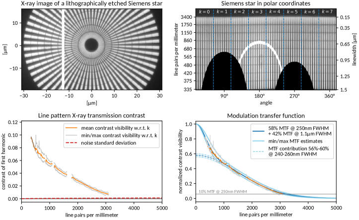
Figure 2: X-ray transmission image of a tungsten based Siemens star (upper left), its representation in polar coordinates (upper right), quantification of frequency dependent transmission contrast (lower left, cf. Eqs. 6–8) and the deduced modulation transfer function (lower right, cf. Eqs. 15–17). The material is not fully absorbing, wherefore the observed contrast of the first harmonic does not exceed 12% (equivalent to 15% contrast for a square wave) in the low frequency limit. The grayscale window of the shown images has therefore been visually adjusted to the object’s contrast. The X-ray image covers a subregion on the detector including a band of 12 insensitive detector columns (white) in between detector tiles, which transforms to a parabola in the polar representation. Likewise, missing top and bottom sections transform to black parabolas. Dashed lines in the polar representation separate individually analyzed sections $k$ (cf. Section 2.2). The expected noise level of the contrast analysis is indicated in red (lower left, cf. Eq. 27)

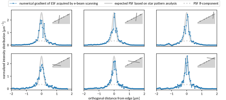
Figure 3: Point spread of the X-ray source’s electron beam determined by numerical differentiation of edge spread curves. The latter are acquired by monitoring X-ray emission while scanning the source’s electron beam over an edge of its structured transmission target. Scanning has been performed at shallow angles with respect to the edge in order to increase the sampling density, and multiple locations within a range of 9 µm along the edge have been addressed. The respective scanning trajectories are indicated in the upper right corner of each graph. Although the edge scans are apparently subject to considerable noise, they are in plausible agreement with the point spread function – indicated in gray – derived previously by imaging a star pattern (cf. Figure 2 and Eq. 18).

Figure 2 (upper left) shows the X-ray projection image of the Siemens star normalized to a flat field image acquired without sample and scaled to the observed transmission contrast. The transmission of the tungsten background in the very center of the pattern ranges at $t_{\min}\approx 0.72$, with a statistical noise of $\text{$\sigma_{I}$}\approx 0.003$. Given the pixel size of $p\approx 0.07\,\text{\textmu m}$, smallest pattern period of $T_{\min}=0.3\text{\textmu m}$, and $N/M=8$ (cf. Section 2.2), the uncertainty of the contrast visibility is found (using Eq. 27) to be smaller than

$$\sigma_{v} \lesssim 0.001\>,$$ (14)

confirming the signal-to-noise ratio to be sufficient for the observed range of contrast visibilities $v\gtrsim 0.005$.

In Figure 2 (upper right), the polar representation of the image is given and annotated with the respective pattern frequencies and line widths ($T/2$) along the radial dimension (cf. Eqs. 2 and 4). The boundaries between the eight angular segments indexed by $k$ and analyzed independently by Eqs. 6–8 are indicated with vertical dashed lines.

The bottom left panel of Fig. 2 shows the deduced mean, minimum and maximum (with respect to $k$) contrast visibilities as a function of pattern frequency. On the bottom right, linear combinations of two Gaussians (shown in different shades of blue) characterizing the high- and low frequency behaviors respectively have been manually fitted to the mean, minimum and maximum modulation transfer characteristic found within the Siemens star. The high frequency component is additionally indicated separately using dashed lines. The frequency dependent contrast reduction (MTF) within the star pattern is apparently well described by this bi-Gaussian model (cf. Fig 2), with

$$\mathrm{MTF}_{\min}(f) \approx 0.56\,e^{-3.56\,(260\,\mathrm{nm})^{2}f^{2}}+0.44\,e^{-3.56\,(1.2\,\text{\textmu m})^{2}f^{2}}$$ (15)

$$\mathrm{MTF}_{\mathrm{mean}}(f) \approx 0.58\,e^{-3.56\,(250\,\mathrm{nm})^{2}f^{2}}+0.42\,e^{-3.56\,(1.1\,\text{\textmu m})^{2}f^{2}}$$ (16)

$$\mathrm{MTF}_{\max}(f) \approx 0.60\,e^{-3.56\,(240\,\mathrm{nm})^{2}f^{2}}+0.40\,e^{-3.56\,(0.9\,\text{\textmu m})^{2}f^{2}}\>.$$ (17)

The point spread function corresponding to $$\mathrm{MTF_{\mathrm{mean}}} (f)$$ is given by (cf. Eq. 9):

$$g_{\,\begin{subarray}{c}\mathrm{mean}\\ \mathrm{MTF}\end{subarray}}(d) \approx 2.1794\,\text{\textmu m}^{-1}e^{-\frac{2.773\,d^{2}}{(250\,\mathrm{nm})^{2}}}+0.3587\,\text{\textmu m}^{-1}e^{-\frac{2.773\,d^{2}}{(1.1\,\text{\textmu m})^{2}}}\>,$$ (18)

with full widths at half maximum

$$\mathrm{FWHM}_{(\mathrm{MTF},\mathrm{hf})} \approx(250\pm 10)\,\mathrm{nm}$$ (19)

$$\mathrm{FWHM}_{(\mathrm{MTF},\mathrm{lf})} \approx(1.1\pm 0.2)\,\text{\textmu m}$$ (20)

of the high frequency (hf) and low frequency (lf) contributions respectively, as determined from the MTF. The wide tail of the point spread contributes, based on the above model fits, $(42\pm 2)\,\%$ of the integral amount of light.

The expected maximal resolution as defined by Eq. 13 ranges at

$$f_{\max} \approx\frac{0.8043}{\mathrm{(250\pm 10)\,\mathrm{nm}}}\approx(3220\pm 130)\,\mathrm{linepairs}/\mathrm{mm}$$ (21)

corresponding to a minimal resolvable linewidth (at 50% duty cycle) of

$$\frac{T_{\min}}{2} \approx\frac{1}{2}\frac{\mathrm{(250\pm 10)\,\mathrm{nm}}}{0.8043}\approx(155\pm 6)\,\mathrm{nm}\,$$ (22)

Due to the longer tailed component of the point spread function as expected from the bi-Gaussian MTF, the actual contrast transfer at $f_{\max}$ is expected to range at $(5.8\pm 0.1)\,\%$.

3.2 PSF from edge scan of the electron focus

Figure 3 compares Eq. 18 to numerically differentiated edge scans of the source’s electron focus. Due to the considerable noise level observed, a total of 6 scans distributed over multiple positions along the edge have been performed (covering a total range of $9\,\text{\textmu m}$ along the edge). Two different scanning directions corresponding to the two available deflection coils have been chosen. The actual scanning motions have been calibrated to spatial units as outlined in Figure 1. The true orientation of the scanned edge has subsequently been determined as a line fit to the transition points of the acquired edge spread functions. The transition points, edge and scanning trajectories are explicitly indicated in Figure 3 along with the observed point spread functions.

Both the narrow and wide components of the PSF as determined previously from the X-ray image of a star pattern are visibly reproduced. Quantitative least squares fits (not shown) of the bi-Gaussian PSF model are however found to exhibit large variations of up to 30% among repeated experiments with respect to all fit parameters, indicating that the edge scans are predominantly suited for qualitative assessments. Given the considered length scales, the pronounced and reproducible noise right at the very edge (i.e., at the very center of the deduced PSF) may have multiple explanations, including in particular actual wear of the tungsten edge due to frequent electron bombardment.

Vanishing in the derivatives shown in Figure 3 is a constant offset within the edge spread functions corresponding to 20% of the total intensity. The respective point spread FWHM of this contribution is inaccessible to the present methodologies and can only be constrained to be either among the observed ones or range above 2 µm based on the unobserved frequencies of the MTF below 340 line pairs per millimeter.

4 Discussion

The analysis of the Siemens star provides experimental data on the frequency dependent contrast reduction in the range between 340 and 3100 line pairs per millimeter. Although the finest structures within the imaged star actually range up to about 3400 line pairs per millimeter, regions at the very end of each patterned band within the star have been intentionally excluded from the analysis due to systematic contrast enhancements caused by radial discontinuities of the bar pattern. The observed contrasts can be well described by a bi-Gaussian (yet single-peak) model of the MTF and the corresponding PSF, which reveals point spread FWHMs of $(250\pm 10)\,\mathrm{nm}$ and $(1.1\pm 0.2)\,\text{\textmu m}$ for the narrow and wide components of the PSF respectively. The narrow PSF component determining the maximal achievable imaging resolution thereby contributes about half of the total X-ray emission, and further ranges at the better end of expectations from Monte Carlo simulations of X-ray generation in thin target layers [19]. These results are further supported by an independent assessment of the X-ray source’s electron focal spot obtained by scanning the electron beam over an edge of the source’s transmission target and analyzing the variation in X-ray emission. Despite being less suited for quantitative analyses (in accordance with the initial motivation for the use of periodic patterns as opposed to edges), the direct observation of point spread shows to be consistent with the observed modulation transfer within the star pattern and in particular confirms the two-component nature of the PSF. In addition, a contribution of 20% of the total emitted intensity can be observed when focusing the electron beam on the bare diamond vacuum window, which may originate from the vacuum window itself, from de-focused electrons hitting distant target regions, or from residual metals on the vacuum window. Bremsstrahlung generated within the vacuum window (which also serves as the structured target’s substrate) is indeed expected from Monte Carlo simulations [32], and would, due to the window’s much larger thickness as compared to the actual target material, indeed exhibit a considerably wider FWHM as compared to the main contribution from the target layer.

5 Conclusion

The modulation transfer function (MTF) and respective point spread function (PSF) characterizing the imaging performance of the ntCT nano-tomography system and the employed Excillum NanoTube X-ray source have been determined both by means of Fourier analysis of the image of a Siemens star and edge scans of the focused electron beam over the source’s structured tungsten target. Within the frequency range of 340 to 3100 line pairs per millimeter a bi-Gaussian (yet single-peak) point spread shape is found, whereof the narrow contribution exhibits a FWHM of $(250\pm 10)\,\mathrm{nm}$, allowing for imaging applications with resolutions up to $150\,\mathrm{nm}$. About half of the total X-ray intensity is found to be emitted from this narrow focal point.

6 Appendix: noise analysis

Particularly with respect to the highest frequencies at the resolution limit, quantification of the signal-to-noise ratio of the present contrast visibility analyses is critical for multiple reasons: First, the analysis of (non-negative) amplitude magnitudes (Eq. 7) is susceptible to non-negligible bias whenever the statistical noise is comparable to or even exceeds the actual amplitudes (cf. e.g. [11]). Noise is here expected to increase for smaller structures due to the nature of the Siemens star, with smaller structures also covering less detector area. Smaller structures are finally expected to exhibit smaller amplitudes due to the imaging system’s modulation transfer properties. The expected noise variance of $\sigma_{v}^{(k)}(r)$ of $v^{(k)}(r)$ with respect to the radial distance $r$ from the center and the related pattern frequency $f(r)=1/T(r)$ (cf. Eqs. 2–4) shall thus be explicitly related to the directly quantifiable variance $\sigma_{I}^{2}$ of the original image intensities.

First, the noise properties of $a_{1}^{(k)}(r)$ and $t^{(k)}(r)$ need to be considered. Given that the integrals of Eqs. 7–8 will generally be evaluated as finite sums over discrete intensity samples $I(r,\varphi_{i})$ at $i\in\{1,...,n\}$, the following holds under the assumption of uncorrelated Gaussian noise and equidistant phases $\varphi_{i}$ covering multiples of a full period of the considered pattern:

$$\sigma_{a_{1}}^{(k)}(r) \approx\sum_{i}\sqrt{\left(\frac{\partial a_{1}^{(k)}}{\partial I(r,\varphi_{i})}\,\sigma_{I}\right)^{2}}=\sqrt{\frac{2}{n}}\,\sigma_{I}$$ (23)

$$\sigma_{t}^{(k)}(r) \approx\sum_{i}\sqrt{\left(\frac{\partial a_{1}^{(k)}}{\partial I(r,\varphi_{i})}\,\sigma_{I}\right)^{2}}=\sqrt{\frac{1}{n}}\,\sigma_{I}\>,$$ (24)

with $n$ denoting the number of intensity samples (i.e., detector pixels) contributing to the evaluation of $v^{(k)}(r)$ at a given radius $r$ of the star pattern. The number of actual detector pixels contributing can be straight forwardly estimated by comparing the lengths of a considered bar pattern (i.e., $N/M$ periods of length $T(r)=1/f(r)$) to the known pixel size $p$ of the original (prior to upsampling) images:

$$n \approx\frac{N\,T(r)}{M\,p}\>.$$ (25)

Based on the orthogonality of the Fourier basis, the noise on $a_{1}^{(k)}(r)$ and $t^{(k)}(r)$ remains uncorrelated, such that

$$\sigma_{v}^{(k)}(r)\approx\sqrt{\left(\frac{\partial v^{(k)}}{\partial a_{1}^{(k)}(r)}\,\sigma_{a_{1}}^{(k)}(r)\right)^{2}+\left(\frac{\partial v^{(k)}}{\partial t(r)}\,\sigma_{t}^{(k)}(r)\right)^{2}}\approx\frac{\sigma_{a_{1}}^{(k)}(r)}{t^{(k)}(r)}\qquad\text{for }a_{1}^{(k)}(r)\ll t^{(k)}(r)$$ (26)

holds analogously.

The largest noise variance on $v^{(k)}(T(r))$ is thus expected for the smallest pattern period $T_{\min}$ (or highest frequency $f_{\max}=1/T_{\min}$) within in the Siemens star:

$$\sigma_{v}(f=1/T) \lesssim\frac{1}{t_{\min}}\sqrt{2\frac{M}{N}\frac{p}{T_{\min}}}\sigma_{I}\>,$$ (27)

where $t_{\min}$ characterizes the minimal mean transmission value observed within the star pattern. A lower bound may e.g. be determined from the unstructured center region (cf. Figure 2). Given that the properties $\sigma_{I}$ (image noise standard deviation) and $t_{\min}$ (lower bound on the mean transmission of the star pattern) are representative for the entire image, the upper bound on $\sigma_{v}$ given by Eq. 27 is independent of the considered angular section $k$.

References

- [1] L. Brownlow, S. Mayo, P. Miller, and J. Sheffield-Parker. Towards 50-nanometre resolution with an sem-hosted x-ray microscope. Microscopy and Analysis, 112:13–15, 2006.
- [2] P. Bruyndonckx, A. Sasov, and B. Pauwels. Towards sub-100-nm x-ray microscopy for tomographic applications. Powder Diffraction, 25(2):157–160, 2010.
- [3] A. E. Burgess. Interpretation of star test pattern images. Med. Phys., 4(1):1–8, 1977.
- [4] M. Busse, M. Müller, M. A. Kimm, S. Ferstl, S. Allner, K. Achterhold, J. Herzen, and F. Pfeiffer. Three-dimensional virtual histology enabled through cytoplasm-specific x-ray stain for microscopic and nanoscopic computed tomography. PNAS, 115(10):2293–2298, 2018.
- [5] T. Donath, S. Brandstetter, L. Cibik, S. Commichau, P. Hofer, M. Krumrey, B. Lüthi, S. Marggraf, P. Müller, M. Schneebeli, C. Schulze-Briese, and J. Wernecke. Characterization of the pilatus photon-counting pixel detector for x-ray energies from 1.75 kev to 60 kev. J. Phys.: Conf. Ser., 425:062001, 2013.
- [6] T. Dreier, U. Lundström, and M. Bech. Super-resolution x-ray imaging with hybrid pixel detectors using electromagnetic source stepping. J. Inst., 15:C03002, 2020.
- [7] M. Eckermann, M. Töpperwien, A. L. Robisch, F. van der Meer, C. Stadelmann, and T. Salditt. Phase-contrast x-ray tomography of neuronal tissue at laboratory sources with submicron resolution. J. Med. Imag., 7(1):013502, 2020.
- [8] C. Fella, J. Dittmann, D. Müller, T. Donath, T. Tuohimaa, and R. Hanke. Implementation of a computed tomography system based on a laboratory-based nanofocus x-ray source. Microscopy and Microanalysis, 24(S2):234–235, 2018.
- [9] A. González-López. Effect of noise on mtf calculations using different phantoms. Med. Phys., 45(5):1889–1898, 2018.
- [10] J. Graetz, D. Müller, A. Balles, T. Tuohimaa, T. Donath, and C. Fella. ntct: submicrometer laboratory x-ray microtomography down to 0.2µm resolution. Proc. 6th Intl. CT-Meeting, page 514–517, 2020.
- [11] H. Gudbjartsson and S. Patz. The rician distribution of noisy mri data. Magn. Reson. Med., 34(6):910–914, 1995.
- [12] R. Hanke, F. Nachtrab, S. Burtzlaff, V. Voland, N. Uhlmann, F. Porsch, and W. Johansson. Setup of an electron probe micro analyzer for highest resolution radioscopy. Nuc. Inst. Meth. A, 607(1):173–175, 2009.
- [13] B. Henrich, A. Bergamaschi, C. Broennimann, R. Dinapoli, E. F. Eikenberry, I. Johnson, M. Kobas, P. Kraft, A. Mozzanica, and B. Schmitt. Pilatus: A single photon counting pixel detector for x-ray applications. Nuc. Inst. Meth. A, 607(1):247–249, 2009.
- [14] R. Horstmeyer, R. Heintzmann, G. Popescu, L. Waller, and C. Yang. Standardizing the resolution claims for coherent microscopy. Nature Photon, 10:68–71, 2016.
- [15] C. Loebich, D. Wueller, B. Klingen, and A. Jaeger. Digital camera resolution measurement using sinusoidal siemens stars. SPIE Electronic Imaging Conference, 6502:65020N, 2007.
- [16] E. Maire and P. J. Withers. Quantitative x-ray tomography. Int. Mat. Rev., 59(1):1–43, 2014.
- [17] K. Masaoka, M. Sugawara, and Y. Nojiri. Multidirectional mtf measurement of digital image acquisition devices. Digital Photography IV, SPIE, 7537:75370V, 2010.
- [18] S. C. Mayo, T. J. Davis, T. E. Gureyev, P. R. Miller, D. Paganin, A. Pogany, A. W. Stevenson, and S. W. Wilkins. X-ray phase-contrast microscopy and microtomography. Opt. Express, 11(19):2289–2302, 2003.
- [19] F. Nachtrab, T. Ebensperger, B. Schummer, F. Sukowski, and R. Hanke. Laboratory x-ray microscopy with a nano-focus x-ray source. J. Inst., 6:C11017, 2011.
- [20] F. Nachtrab, M. Firsching, C. Speier, N. Uhlmann, P. Takman, T. Tuohimaa, C. Heinzl, J. Kastner, D. H. Larsson, A. Holmberg, G. Berti, M. Krumm, and Sauerwein C. Nanoxct: development of a laboratory nano-ct system. Proc SPIE Dev. in X-ray Tomography IX, page 92120L, 2014.
- [21] J. Otón, C. O. S. Sorzano, R. Marabini, E. Pereiro, and J. M. Carazo. Measurement of the modulation transfer function of an x-ray microscope based on multiple fourier orders analysis of a siemens star. Opt. Express, 23(8):9567–9572, 2015.
- [22] L. A. Gomes Perini, P. Bleuet, J. Filevich, W. Parker, B. Buijsse, and L. F. Tz. Kwakman. Developments on a sem-based x-ray tomography system: Stabilization scheme and performance evaluation. Rev. Sci. Instrum., 88(6):063706, 2017.
- [23] G. Probst, Q. Hou, R. Pauwels, B. Boeckmans, Y. Xiao, and W. Dewulf. Focal spot characterization of an industrial x-ray ct scanner. Intl. Symp. on Digital Industrial Radiology and Computed Tomography (DIR) 2019, 2019.
- [24] S. Rehbein, P. Guttmann, S. Werner, and G. Schneider. Characterization of the resolving power and contrast transfer function of a transmission x-ray microscope with partially coherent illumination. Opt. Express, 20(6):5830–5839, 2012.
- [25] M. Salamon, R. Hanke, P. Krüger, F. Sukowski, N. Uhlmann, and V. Voland. Comparison of different methods for determining the size of a focal spot of microfocus x-ray tubes. Nuc. Inst. Meth. A, 591(1):54–58, 2008.
- [26] C. Seim, J. Baumann, H. Legall, C. Redlich, I. Mantouvalou, G. Blobel, H. Stiel, and B. Kanngießer. Laboratory full-field transmission x-ray microscopy. Proc. SPIE, 8678:867808, 2012.
- [27] P. Stahlhut, K. Dremel, J. Dittmann, J. M. Engel, S. Zabler, A. Hoelzing, and R. Hanke. First results on laboratory nano-ct with a needle reflection target and an adapted toolchain. Proc SPIE, 9967:99670I, 2016.
- [28] P. A. C. Takman, H. Stollberg, G. A. Johansson, A. Holmberg, M. Lindblom, and H. M. Hertz. High-resolution compact x-ray microscopy. J. Microscopy, 226(2):175–181, 2007.
- [29] D. Weiß, Q. Shi, and C. Kuhn. Measuring the 3d resolution of a micro-focus x-ray ct setup. Conference on Industrial Computed Tomography (iCT), page 345–353, 2012.
- [30] P. J. Withers. X-ray nanotomography. Materials Today, 10(12):26–34, 2007.
- [31] S. Zabler, M. Ullherr, C. Fella, R. Schielein, O. Focke, B. Zeller-Plumhoff, P. Lhuissier, W. DeBoever, and R. Hanke. Comparing image quality in phase contrast sub x-ray tomography—a round-robin study. Nuc. Inst. Meth. A, 951(21):162992, 2020.
- [32] R. Zhou, X. Zhou, X. Li, Y. Cai, and F. Liu. Study of the microfocus x-ray tube based on a point-like target used for micro-computed tomography. PLoS ONE, 11(6):e0156224, 2016.