A compute-bound formulation of Galerkin model reduction for linear time-invariant dynamical systems

Abstract

This work aims to advance computational methods for projection-based reduced-order models (ROMs) of linear time-invariant (LTI) dynamical systems. For such systems, current practice relies on ROM formulations expressing the state as a rank-1 tensor (i.e., a vector), leading to computational kernels that are memory bandwidth bound and, therefore, ill-suited for scalable performance on modern architectures. This weakness can be particularly limiting when tackling many-query studies, where one needs to run a large number of simulations. This work introduces a reformulation, called rank-2 Galerkin, of the Galerkin ROM for LTI dynamical systems which converts the nature of the ROM problem from memory bandwidth to compute bound. We present the details of the formulation and its implementation, and demonstrate its utility through numerical experiments using, as a test case, the simulation of elastic seismic shear waves in an axisymmetric domain. We quantify and analyze performance and scaling results for varying numbers of threads and problem sizes. Finally, we present an end-to-end demonstration of using the rank-2 Galerkin ROM for a Monte Carlo sampling study. We show that the rank-2 Galerkin ROM is one order of magnitude more efficient than the rank-1 Galerkin ROM (the current practice) and about $970$ times more efficient than the full-order model, while maintaining accuracy in both the mean and statistics of the field.

68W01, 68W10, 68W40, 65M06, 65M22, 65L05, 65L10, 65F50, 37N99, 37N10, 86A15, 86A17, 86A22, 65C05, 74J25, 74J15 37M05,

1 Introduction

The “extreme-scale” computing era in which we are living, also referred to by many as the dawn of exascale computing (the capability to perform $10^{18}$ floating-point operations per second), is enabling a shift in the paradigm within which we approach new problems. We no longer target few simulations executed for specific choices of parameters and conditions, but are increasingly interested in exploiting high-fidelity models to generate ensembles of runs to tackle many-query problems, such as uncertainty quantification (UQ). These typically require large sets of runs to adequately characterize the effect of uncertainties in parameters and operating conditions on the system response. Such an approach is key to solve, e.g., design optimization and parameter-space exploration problems.

If the system of interest is computationally expensive to query—for example very high-fidelity models for which a single run can consume days or weeks on a supercomputer—its use for many-query problems is impractical or even impossible. Consequently, analysts often turn to surrogate models, which replace the high-fidelity model with a lower-cost, lower-fidelity counterpart. To be useful, surrogate models should meet accuracy, speed, and certification requirements. Accuracy ensures that the surrogate produces a sufficiently small error in target quantities of interest. The maximum acceptable error is typically defined by the user and is problem-dependent. Speed ensures that the surrogate evaluates much more rapidly than the full-order model, and one typically has to consider a tradeoff between speed and accuracy. Certification ensures that the error (and its bounds) introduced by the surrogate can be properly quantified and characterized. We additionally note that it is often desirable that surrogate models preserve important physical properties, such as Lagrangian or Hamiltonian structure, or mass conservation.

Broadly speaking, surrogate models fall under three categories, namely (a) data fits, which construct an explicit mapping (e.g., using polynomials, Gaussian processes) from the system’s parameters (i.e., inputs) to the system response of interest (i.e., outputs), (b) lower-fidelity models, which simplify the high-fidelity model (e.g., by coarsening the mesh, employing a lower finite-element order, or neglecting physics), and (c) projection-based reduced-order models (ROMs), which reduce the number of degrees of freedom in the high-fidelity model though a projection process. The main advantage of ROMs is that they apply a projection process directly to the equations governing the high-fidelity model, thus enabling stronger guarantees (e.g., of structure preservation, of accuracy via adaptivity) and more robust error analyses, e.g., via a priori or a posteriori error bounds. We can identify two main research branches within the field of ROMs, one addressing nonlinear systems and the other focusing on linear systems. In this work, we focus on the latter, more specifically linear time-invariant (LTI) dynamical systems, which are linear in state but have an arbitrary nonlinear parametric dependence.

Projection-based model reduction of LTI systems is a mature field in terms of methodological and algorithmic development [9, 6], but we argue that it lags behind in terms of implementation and computational advancement. On the one hand, numerous ROM techniques have been developed for such systems accounting for, e.g., observability and controllability [51, 75, 52, 42], $\mathcal{H}_{2}$-optimality [24, 76, 31], structure preservation [41, 10], and non-affine parametric dependence [13, 23]. Furthermore, these ROMs can be certified via a priori and a posteriori error analysis [58, 60, 61, 40, 64, 73, 51, 9, 25]. As a result, it is possible to construct stable, accurate, and certified ROMs for a wide class of LTI systems. On the other hand, the computational aspects of solving these systems efficiently, especially in the context of many-query problems, has not achieved a comparable level of maturity. This statement is grounded in the fact that the standard formulation of ROMs for LTI dynamical systems expresses the state as a rank-1 tensor (i.e., a vector), see [9, 6], which makes the corresponding computational kernels memory bandwidth bound (as we will show in § 4.2), and therefore not well-suited for modern multi-core processors or accelerators.

This work presents our contribution towards improving the computational efficiency of ROMs for LTI systems. We present and demonstrate a reformulation of the ROM problem for LTI dynamical systems such that we change its nature from memory bandwidth bound to compute bound, making it more suitable for modern multi- and many-core computing nodes. More specifically, we believe this work makes the following contributions:

• a new ROM formulation, referred to as “rank-2 Galerkin”, for LTI dynamical systems that is efficient for many-query problems, and comprehensive numerical results to demonstrate its performance and scalability;

• a new open-source C++ code, developed from the ground up using the performance-portable Kokkos programming model [14], to simulate the evolution of seismic shear waves in an axi-symmetric domain;

• detailed numerical examples based on the shear wave problem to demonstrate the rank-2 Galerkin ROM (which, to the best of our knowledge, also constitutes the first application of ROMs to seismic shear waves).

The paper is organized as follows. In § 2, we present the formulation and discuss the advantages and disadvantages of various Galerkin ROM formulations, in § 3 we present the test case chosen for our numerical experiments and its implementation details, and in § 4 we describe the results. Conclusions and outlook to future work are presented in § 5.

2 Mathematical Formulation

We focus on problems expressible in semi-discrete form as

(1) $$\frac{d\boldsymbol{x}}{dt}(t;\boldsymbol{\eta},\boldsymbol{\mu})=\mathbf{A}(\boldsymbol{\eta})\boldsymbol{x}(t;\boldsymbol{\eta},\boldsymbol{\mu})+\boldsymbol{f}(t;\boldsymbol{\eta},\boldsymbol{\mu}),$$

where $\boldsymbol{x}:[0,t_{final}]\times\mathcal{D}_{\eta}\times\mathcal{D}_{\mu}\rightarrow\mathbb{R}^{N}$ is the state, $\boldsymbol{x}(0;\boldsymbol{\eta},\boldsymbol{\mu})=\boldsymbol{x}^{0}$ is the initial state, $\mathbf{A}(\boldsymbol{\eta})\in\mathbb{R}^{N\times N}$ is the discrete system matrix parametrized by ${\boldsymbol{\eta}\in\mathcal{D}_{\eta}\subset\mathbb{R}^{N_{\boldsymbol{\eta}}}}$, $\boldsymbol{f}:[0,t_{final}]\times\mathcal{D}_{\eta}\times\mathcal{D}_{\mu}\rightarrow\mathbb{R}^{N}$ is the time-dependent forcing term also parametrized by $\boldsymbol{\mu}\in\mathcal{D}_{\mu}\subset\mathbb{R}^{N_{\boldsymbol{\mu}}}$, and $t_{final}>0$ is the final time. We assume $N$ to be large, e.g., hundreds of thousands or more, which is a suitable assumption for real applications. Since the state is a rank-1 tensor (i.e., a vector), hereafter we refer to a formulation of the form (1) as the rank-1 full-order model (Rank1FOM).

The above formulation is linear in the state, but can have an arbitrary nonlinear parametric dependence. No assumption is made on the original problem leading to (1), thus making it applicable to systems obtained from the spatial discretization of a partial differential equation (PDE) or problems that are inherently discrete. We assume the discrete system matrix, $\mathbf{A}(\boldsymbol{\eta})$, to be sparse, with its sparsity pattern depending on the problem and chosen discretization. We remark that the formulation above, as well as what we present below, is also applicable to the case where $\mathbf{A}(\boldsymbol{\eta})$ has an affine parametrization. We purposefully split the parametric dependence into $\boldsymbol{\eta}$ and $\boldsymbol{\mu}$ to highlight their different roles: $\boldsymbol{\mu}$ includes only the parameters that impact the forcing, while $\boldsymbol{\eta}$ includes all the others. This separation will be helpful for the formulations in the sections below.

2.1 Applicability and representative applications

A wide range of problems in science and engineering have governing equations of the form (1). For example, the dynamics of a deforming structure can often be modeled as linear, but the load distribution on the structure can be parametrized by nonlinear functions. This is typical in the field of aeroelasticity, where the aircraft structure is modeled by a linear PDE and the aerodynamic loads on the aircraft are highly nonlinear [17, 49, 22, 7, 12]. Similarly, the temperature of a structure may often be modeled with the linear heat equations and boundary conditions set by nonlinear temperature distributions and/or heat loads [33]. Nonlinear boundary conditions commonly arise in a number of applications including electronics cooling [79, 5], building thermal management [20], and industrial heat exchanger design [62]. Neutral particle (neutron, photon, etc.) transport, when simulated via deterministic methods, often gives rise to linear systems of this form [43, 67]. Acoustic waves are also modeled with a linear PDE, but can have a number of nonlinear sources, most notably turbulent shear layers that arise in the wakes of cars, aircraft, and other moving objects [46, 21, 56, 47]. Linear circuit models are ubiquitous in electrical engineering and evolve time according to ODEs of the form (1) while commonly being driven by complex nonlinear forcing functions [72, 16, 80].

2.2 Galerkin ROM

Projection-based ROMs generate approximate solutions of the full-order model (1) by (a) restricting the state to live in a low-dimensional (affine) trial subspace, and (b) enforcing the residual of the ODE to be orthogonal to a low-dimensional test subspace. In this work, we limit the scope to the Galerkin ROM, which is one of the most popular methodologies (another one is, e.g., Petrov-Galerkin).

The Galerkin ROM approximates solutions $\tilde{\boldsymbol{x}}(t;\boldsymbol{\eta},\boldsymbol{\mu})\approx\boldsymbol{x}(t;\boldsymbol{\eta},\boldsymbol{\mu})$ in a low-dimensional affine trial subspace, ${\tilde{\boldsymbol{x}}(t;\boldsymbol{\eta},\boldsymbol{\mu})\in\mathcal{V}+\boldsymbol{x}_{\text{ref}}(\boldsymbol{\eta},\boldsymbol{\mu})}$, with ${\text{dim}(\mathcal{V})=K}$ such that $K\ll N$ and where $\boldsymbol{x}_{\text{ref}}(\boldsymbol{\eta},\boldsymbol{\mu})\in\mathbb{R}^{N}$ defines the affine offset (also called the reference state). Here, we take $\mathcal{V}=\text{Range}(\boldsymbol{\Phi})$, where ${\boldsymbol{\Phi}\equiv\begin{bmatrix}\boldsymbol{\phi}_{1}&\cdots&\boldsymbol{\phi}_{K}\end{bmatrix}}$ comprises $K$-orthonormal basis vectors. Such a basis may be obtained, for example, by proper orthogonal decomposition [65, 11]. For ${t\in[0,t_{final}]}$, ${\boldsymbol{\eta}\in\mathcal{D}_{\eta}}$, ${\boldsymbol{\mu}\in\mathcal{D}_{\mu}}$, the FOM solution is approximated as

(2) $$\boldsymbol{x}(t;\boldsymbol{\eta},\boldsymbol{\mu})\approx\tilde{\boldsymbol{x}}(t;\boldsymbol{\eta},\boldsymbol{\mu})=\boldsymbol{\Phi}\hat{\boldsymbol{x}}(t;\boldsymbol{\eta},\boldsymbol{\mu})+\boldsymbol{x}_{\text{ref}}(\boldsymbol{\eta},\boldsymbol{\mu}),$$

where $\hat{\boldsymbol{x}}:[0,t_{final}]\times\mathcal{D}_{\eta}\times\mathcal{D}_{\mu}\rightarrow\mathbb{R}^{K}$ are referred to as the generalized coordinates. The initial state for the generalized coordinates can be computed by projecting the FOM initial condition, i.e., using $\hat{\boldsymbol{x}}(0;\boldsymbol{\eta},\boldsymbol{\mu})=\boldsymbol{\Phi}^{T}\boldsymbol{x}(0;\boldsymbol{\eta},\boldsymbol{\mu})$.

Equipped with (2), the Galerkin ROM proceeds by restricting the residual to be orthogonal to the trial space yielding the following reduced-order model

(3) $$\frac{d\hat{\boldsymbol{x}}}{dt}(t;\boldsymbol{\eta},\boldsymbol{\mu})=\hat{\mathbf{A}}(\boldsymbol{\eta})\hat{\boldsymbol{x}}(t;\boldsymbol{\eta},\boldsymbol{\mu})+\hat{{\boldsymbol{f}}}(t;\boldsymbol{\eta},\boldsymbol{\mu})+\hat{{\boldsymbol{x}}}_{\text{ref}}(\boldsymbol{\eta},\boldsymbol{\mu})$$

where $\hat{\mathbf{A}}(\boldsymbol{\eta})\equiv\boldsymbol{\Phi}^{T}\mathbf{A}(\boldsymbol{\eta})\boldsymbol{\Phi}\in\mathbb{R}^{K\times K}$ is the reduced (dense) system matrix, $\hat{{\boldsymbol{f}}}(t;\boldsymbol{\eta},\boldsymbol{\mu})=\boldsymbol{\Phi}^{T}\boldsymbol{f}(t;\boldsymbol{\eta},\boldsymbol{\mu})$ is the reduced forcing, $\hat{{\boldsymbol{x}}}_{\text{ref}}(\boldsymbol{\eta},\boldsymbol{\mu})=\boldsymbol{\Phi}^{T}\mathbf{A}(\boldsymbol{\eta})\boldsymbol{x}_{\text{ref}}(\boldsymbol{\eta},\boldsymbol{\mu})$ is the reduced reference state, and we used the fact that $\boldsymbol{\Phi}^{T}\boldsymbol{\Phi}={\boldsymbol{I}}$. A schematic of the above sysyem is shown in Figure 1. When the basis is not orthogonal, the transpose operations in (3) should be replaced with the pseudo-inverse. Note that the affine offset, $\boldsymbol{x}_{\text{ref}}(\boldsymbol{\eta},\boldsymbol{\mu})$, is introduced for generality, but it not always necessary: when unused or null, it simply drops out of the formulation. Hereafter we refer to a system of the form (3) as the rank-1 Galerkin ROM (Rank1Galerkin).

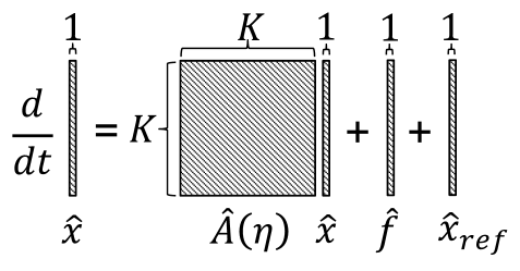
Figure 1: Schematic of the rank-1 Galerkin formulation discussed in Eq. 3.

The last term on the right in (3), $\hat{{\boldsymbol{x}}}_{\text{ref}}(\boldsymbol{\eta},\boldsymbol{\mu})=\boldsymbol{\Phi}^{T}\mathbf{A}(\boldsymbol{\eta})\boldsymbol{x}_{\text{ref}}(\boldsymbol{\eta},\boldsymbol{\mu})$, can be efficiently evaluated since it is time-independent and only needs to be computed once for a given choice of $\boldsymbol{\eta}$. The term $\hat{{\boldsymbol{f}}}(t;\boldsymbol{\eta},\boldsymbol{\mu})=\boldsymbol{\Phi}^{T}\boldsymbol{f}(t;\boldsymbol{\eta},\boldsymbol{\mu})$, despite being seemingly more challenging because of its time-dependence, can also be computed efficiently by considering two scenarios, namely one where $\boldsymbol{f}\in\mathbb{R}^{N}$ is a dense vector and one where it is sparse, with just a few non-zero elements. In the former case, since $K$ is sufficiently small, the best approach would be to precompute and store the product $\boldsymbol{\Phi}^{T}\boldsymbol{f}(t;\boldsymbol{\eta},\boldsymbol{\mu})$ for all the target times over $[0,t_{final}]$. For the other scenario, i.e. a sparse forcing, one can exploit its sparsity pattern at each time $t$ by operating only on the corresponding rows of $\boldsymbol{\Phi}$. This allows one to avoid pre-computing the forcing at all times while maintaining computational efficiency since only a few elements must be operated on.

2.3 Rank-1 Formulation Analysis

The Rank1FOM and Rank1Galerkin formulations are suitable when the objective is to perform a few individual cases, but become inefficient for many-query scenarios involving large ensembles of runs on modern architectures. The reason is that computing the right-hand side of both Rank1FOM and Rank1Galerkin requires memory bandwidth-bound kernels, which impede an optimal/full utilization of a node’s computing resources, especially on modern multi- and many-core computer architectures [30, 78, 19]. A partial solution would be to run the simulations in parallel, as demonstrated in [77], but the individual runs in this approach would still be of the same nature.

Indeed, the Rank1FOM in (1) is characterized by a standard sparse-matrix vector ( spmv) product, which is well-known to be memory bandwidth bound due to its low compute intensity regardless of its sparsity pattern, see e.g. [8, 19]. Defining the computational intensity, $I$, of a kernel as the ratio between flops and memory access (bytes), the spmv kernel has approximately $I\approx nnz/(6N+2+10nnz)$, where $nnz$ is the number of non-zero elements [8, 19].

For the Rank1Galerkin in (3), the defining term is the product $\hat{\mathbf{A}}(\boldsymbol{\eta})\hat{\boldsymbol{x}}(t;\boldsymbol{\eta},\boldsymbol{\mu})$ of the reduced system matrix with the vector of generalized coordinates, which requires a dense general matrix vector ( gemv) product. This kernel is also memory bandwidth bound with an approximate computational intensity $I\approx 1/4$ [53], when the matrix is square as in (3).

2.4 Rank-2 Formulation

In light of the previous discussion, we now present an alternative formulation and implementation that is computationally more efficient for many-query problems with respect to the parameter $\boldsymbol{\mu}$ on modern many-core architectures. Let $\boldsymbol{X}:[0,t_{final}]\times\mathcal{D}_{\eta}\times\mathcal{D}_{\mu}^{M}\rightarrow\mathbb{R}^{N\times M}$ represent a set of $M$ trajectories for the FOM

$$\boldsymbol{X}(t;\boldsymbol{\eta},\mathcal{M})\equiv\begin{bmatrix}\boldsymbol{x}_{1}(t;\boldsymbol{\eta},{\boldsymbol{\mu}}_{1})&\ldots&\boldsymbol{x}_{M}(t;\boldsymbol{\eta},{\boldsymbol{\mu}}_{M})\end{bmatrix},$$

for a given choice of $\boldsymbol{\eta}$ and where $\mathcal{M}={\boldsymbol{\mu}}_{1},\ldots,{\boldsymbol{\mu}}_{M}$ is the set of parameters defining the $M$ forcing realizations driving the trajectories of interest.

Similarly to (1), we can express the dynamics of these FOM trajectories as

(4) $$\frac{d\boldsymbol{X}}{dt}(t;\boldsymbol{\eta},\mathcal{M})=\mathbf{A}(\boldsymbol{\eta})\boldsymbol{X}(t;\boldsymbol{\eta},\mathcal{M})+\boldsymbol{F}(t;\boldsymbol{\eta},\mathcal{M}),$$

where $\boldsymbol{X}(0;\boldsymbol{\eta},\mathcal{M})=\begin{bmatrix}\boldsymbol{x}_{1}(0;\boldsymbol{\eta},{\boldsymbol{\mu}}_{1})&\cdots&\boldsymbol{x}_{M}(0;\boldsymbol{\eta},{\boldsymbol{\mu}}_{M})\end{bmatrix}$ is the initial condition, and the forcing contribution is $\boldsymbol{F}(t;\boldsymbol{\eta},\mathcal{M})\equiv\begin{bmatrix}\boldsymbol{f}(t;\boldsymbol{\eta},{\boldsymbol{\mu}}_{1})&\cdots&\boldsymbol{f}(t;\boldsymbol{\eta},{\boldsymbol{\mu}}_{M})\end{bmatrix}$. We refer to the system of the form (4) as the rank-2 FOM (Rank2FOM). The Rank1FOM in (1) can be seen as a special case of Eq. (4) with $M=1$.

To derive the corresponding Galerkin ROM, we approximate the state as

$$\boldsymbol{X}(t;\boldsymbol{\eta},\mathcal{M})\approx\tilde{\boldsymbol{X}}(t;\boldsymbol{\eta},\mathcal{M})\equiv\boldsymbol{\Phi}\hat{\boldsymbol{X}}(t;\boldsymbol{\eta},\mathcal{M})+{\boldsymbol{X}}_{\text{ref}}(\boldsymbol{\eta},\mathcal{M}),$$

where ${\boldsymbol{X}}_{\text{ref}}(\boldsymbol{\eta},\mathcal{M})\equiv\begin{bmatrix}\boldsymbol{x}_{\text{ref}}(\boldsymbol{\eta},{\boldsymbol{\mu}}_{1})&\cdots&\boldsymbol{x}_{\text{ref}}(\boldsymbol{\eta},{\boldsymbol{\mu}}_{M})\end{bmatrix}\in\mathbb{R}^{N\times M}$, and applying Galerkin projection we obtain

(5) $$\frac{d\hat{\boldsymbol{X}}}{dt}(t;\boldsymbol{\eta},\mathcal{M})=\hat{\mathbf{A}}(\boldsymbol{\eta})\hat{\boldsymbol{X}}(t;\boldsymbol{\eta},\mathcal{M})+\hat{{\boldsymbol{\boldsymbol{F}}}}(t;\boldsymbol{\eta},\boldsymbol{\mu})+\hat{{\boldsymbol{X}}}_{\text{ref}}(\boldsymbol{\eta},\mathcal{M}),$$

where $\hat{\boldsymbol{X}}:[0,t_{final}]\times\mathcal{D}_{\eta}\times\mathcal{D}_{\mu}^{M}\rightarrow\mathbb{R}^{K\times M}$ is a rank-2 tensor of time-dependent generalized coordinates, $\hat{{\boldsymbol{\boldsymbol{F}}}}(t;\boldsymbol{\eta},\boldsymbol{\mu})=\boldsymbol{\Phi}^{T}\boldsymbol{F}(t;\boldsymbol{\eta},\mathcal{M})$ is the reduced forcing, $\hat{{\boldsymbol{X}}}_{\text{ref}}(\boldsymbol{\eta},\mathcal{M})=\boldsymbol{\Phi}^{T}\mathbf{A}(\boldsymbol{\eta}){\boldsymbol{X}}_{\text{ref}}(\boldsymbol{\eta},\mathcal{M})$ is the reduced reference state. Figure 2 shows a schematic of the system in (5), which hereafter we refer to the rank-2 Galerkin ROM (Rank2Galerkin).

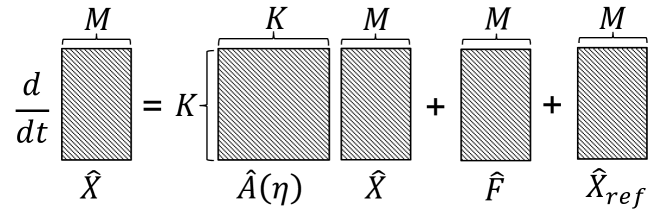
Figure 2: Schematic of the rank-2 Galerkin formulation discussed in Eq. 5.

The term $\boldsymbol{\Phi}^{T}\mathbf{A}(\boldsymbol{\eta}){\boldsymbol{X}}_{\text{ref}}(\boldsymbol{\eta},\mathcal{M})$ can be efficiently evaluated since it is time-independent and only needs to be computed once for a given choice of $\boldsymbol{\eta}$. For the term $\boldsymbol{\Phi}^{T}\boldsymbol{F}(t;\boldsymbol{\eta},\mathcal{M})$, involving the forcing, considerations similar to those drawn for the rank-1 Galerkin in Eq. (3) can be made. The term involving the system matrix is discussed below in more detail.

2.5 Rank-2 Formulation Analysis

The key question we now pose is what advantage, if any, is gained by employing the rank-2 formulation of the FOM and Galerkin ROM over the rank-1 alternatives? The answer is that, when evaluated in a many-query context, Rank2FOM has minimal advantages over Rank1FOM, whereas Rank2Galerkin has major benefits over Rank1Galerkin. We will demonstrate this numerically in § 4.1 and § 4.2, but provide the key insight here.

For the FOM, the Rank2FOM in (4) involves the term $\mathbf{A}(\boldsymbol{\eta})\boldsymbol{X}(t;\boldsymbol{\eta},\mathcal{M})$ requiring a sparse-matrix matrix ( spmm) kernel which, despite having a compute intensity higher than spmv, remains memory bandwidth bound, see e.g. [3, 29]. This implies that Rank2FOM yields some but limited improvements over Rank1FOM.

On the other hand, the Rank2Galerkin in (5) has a major advantage over Rank1Galerkin because it changes the nature of the problem from memory bandwidth to compute bound. This stems from the fact that computing the term $\hat{\mathbf{A}}(\boldsymbol{\eta})\hat{\boldsymbol{X}}(t;\boldsymbol{\eta},\mathcal{M})$ on the right-hand side of Rank2Galerkin in (5) involves a dense general matrix matrix multiplication ( gemm), which has the advantage of performing $\mathcal{O}(n^{3})$ flops on $\mathcal{O}(n^{2})$ memory accesses, yielding a compute bound kernel ([53]). The gemm is one the most studied kernels in dense linear algebra. The approximate computational intensity for gemm is $I\approx K/16$, since the reduced system matrix in Eq. (5) is square with size $K\times K$. This makes the rank-2 Galerkin ROM very well-suited for modern multi- and many-core computing nodes where a high computational intensity is critical for achieving good scaling and efficiency.

Previous work in the field of computational science that is relevant can be found, e.g., in [36, 26, 27, 57]. In [57], the authors propose an “embedded ensemble propagation” technique which exploits modern CPUs’ vectorization and C++ templates to simultaneously propagate multiple samples together. This work, however, does not explicitly address ROMs. In [36, 26], the authors focus on efficient reformulations of the time-dependent Navier-Stokes equations to solve ensenbles. The idea is to employ a reformulation that allows to solve a single linear system for multiple right-hand sides. These studies, however, are tailored to the Navier-Stokes equations. The work in [26] is based on the previous ones, but is particularly relevant to model reduction because the authors discuss an ensemble-based POD Galerkin ROM tailored to the incompressible Navier—Stokes equations for efficiently solving problems characterized by multiple initial conditions and body forces. The idea is based on first performing an ensemble reformulation of the FOM, from which a POD-Galerkin ROM is then constructed. The resulting method is first-order accurate in time, and is tailored to the Navier-Stokes equations. We note that no performance results or comparisons to standard approaches are presented in [26].

3 Test Case Description

As a test case for our numerical experiments, we choose the propagation of global seismic shear waves in spherical coordinates. Shear waves are also called S-waves (or secondary) because they come after P-waves (or primary). The main difference between them is that S waves are transversal (particles oscillate perpendicularly to the direction of wave propagation), while the P waves are longitudinal (particles oscillate in the same direction as the wave). Both P and S waves are body waves, because they travel through the interior of the earth and their trajectories are affected by the material properties, namely density and stiffness.

We specifically focus on the axisymmetric evolution of elastic seismic shear waves. The governing equations in the velocity-stress formulation [32, 34] can be written as:

$$\rho(r,\theta)\frac{\partial v}{\partial t}(r,\theta,t) =\frac{\partial\sigma_{r\phi}}{\partial r}(r,\theta,t)+\frac{1}{r}\frac{\partial\sigma_{\theta\phi}}{\partial\theta}(r,\theta,t)$$

$$+\frac{1}{r}\left(3\sigma_{r\phi}(r,\theta,t)+2\sigma_{\theta\phi}(r,\theta,t)\cot{\theta}\right)+f(r,\theta,t)$$

(6) $$\frac{\partial\sigma_{r\phi}}{\partial t}(r,\theta,t) =G(r,\theta)\left(\frac{\partial v}{\partial r}(r,\theta,t)-\frac{1}{r}v(r,\theta,t)\right)$$

$$\frac{\partial\sigma_{\theta\phi}}{\partial t}(r,\theta,t) =G(r,\theta)\left(\frac{1}{r}\frac{\partial v}{\partial\theta}(r,\theta,t)-\frac{\cot{\theta}}{r}v(r,\theta,t)\right),$$

where $t$ represents time, $r\in[0,r_{earth}]$ is the radial distance bounded by the radius of the earth, $\theta\in[0,\pi]$ is the polar angle, $\rho(r,\theta)$ is the density, $v(r,\theta,t)$ is the velocity, $\sigma_{r\phi}(r,\theta,t)$ and $\sigma_{\theta\phi}(r,\theta,t)$ are the two components of the stress tensor remaining after the axisymmetric approximation, $f(r,\theta,t)$ is the forcing term, and the shear modulus is $G(r,\theta)=v_{s}^{2}(r,\theta)\rho(r,\theta)$, with $v_{s}$ being the shear wave velocity. Note that we assume both the density and shear modulus to only depend on the spatial coordinates. Such a formulation is referred to as 2.5-dimensional because it involves a 2-dimensional spatial domain (a circular sector of the earth) but models point sources with correct 3-dimensional spreading [32, 34].

This is an application of interest to geological and, in particular, seismic modeling. Previous studies focusing on shear waves modeling can be found, e.g., in [32, 15, 34, 74] and references therein.

3.1 Discretization

Since shear waves cannot propagate in liquids, the system of equations in (3) is not applicable to the core region of the earth. Therefore, we solve Eq. (3) in the region bounded between the core-mantle boundary (CMB) located at $r_{cmb}=3,480$ km, and the earth surface located at $r_{earth}=6,371$ km. We discretize the 2D spatial domain using a staggered grid as shown in Figure 3 (a). Staggered grids are typical for seismic modeling and wave problems in general, see [34, 70, 71]. We use a second-order centered finite-difference [34] method for the spatial operators in Eq. (3), which is sufficient for the purposes of this study.

The Rank2FOM formulation of Eq.(3) can be written as

$$\frac{d\boldsymbol{X}_{v}}{dt}(t;\boldsymbol{\eta},\mathcal{M}) =\mathbf{A}_{v}(\boldsymbol{\eta})\boldsymbol{X}_{\sigma}(t;\boldsymbol{\eta},\mathcal{M})+\boldsymbol{F}_{v}(t;\boldsymbol{\eta},\mathcal{M})$$

(7) $$\frac{d\boldsymbol{X}_{\sigma}}{dt}(t;\boldsymbol{\eta},\mathcal{M}) =\mathbf{A}_{\sigma}(\boldsymbol{\eta})\boldsymbol{X}_{v}(t;\boldsymbol{\eta},\mathcal{M}),$$

where $\boldsymbol{X}_{v}\in\mathbb{R}^{N_{v}\times M}$ is the rank-2 state tensor for the velocity degrees of freedom, $\boldsymbol{X}_{\sigma}\in\mathbb{R}^{N_{\sigma}\times M}$ is the rank-2 state tensor with the stresses degrees of freedom, $\mathbf{A}_{v}(\boldsymbol{\eta})\in\mathbb{R}^{N_{v}\times N_{\sigma}}$ is the discrete system matrix for the velocity, $\mathbf{A}_{\sigma}(\boldsymbol{\eta})\in\mathbb{R}^{N_{\sigma}\times N_{v}}$ is the one for the stresses, and $\boldsymbol{F}_{v}(t;\boldsymbol{\eta},\mathcal{M})$ is the rank-2 forcing tensor. In this work, the finite difference scheme adopted leads to system matrices $\mathbf{A}_{v}(\boldsymbol{\eta})$ and $\mathbf{A}_{\sigma}(\boldsymbol{\eta})$ with about four and two non-zeros entries per row, respectively. The corresponding Rank1FOM can be easily obtained from (3.1) by setting $M=1$.

We use the following boundary conditions, similarly to [34]. Directly at the symmetry axis, i.e., $\theta=0$ and $\theta=\pi$, the velocity is set to zero since it undefined here due to the cotangent term in its governing equation. This implies that at the symmetry axis the stress $\sigma_{r\phi}$ is also zero. At the core-mantle boundary and earth surface we impose a free surface boundary condition (i.e., waves fully reflect), by setting the zero-stress condition ${\sigma_{r\phi}(r_{cmb},\theta,t)=\sigma_{r\phi}(r_{earth},\theta,t)=0}$. Note that this condition on the stress implicitly defines the velocity at the core-mantle boundary and earth surface and, therefore, no boundary condition on the velocity itself must be set there. We remark that, differently than [34], we do not rely on ghost points to impose boundary conditions, because these are already accounted for when assembling the system matrices $\mathbf{A}_{v}(\boldsymbol{\eta})$ and $\mathbf{A}_{\sigma}(\boldsymbol{\eta})$.

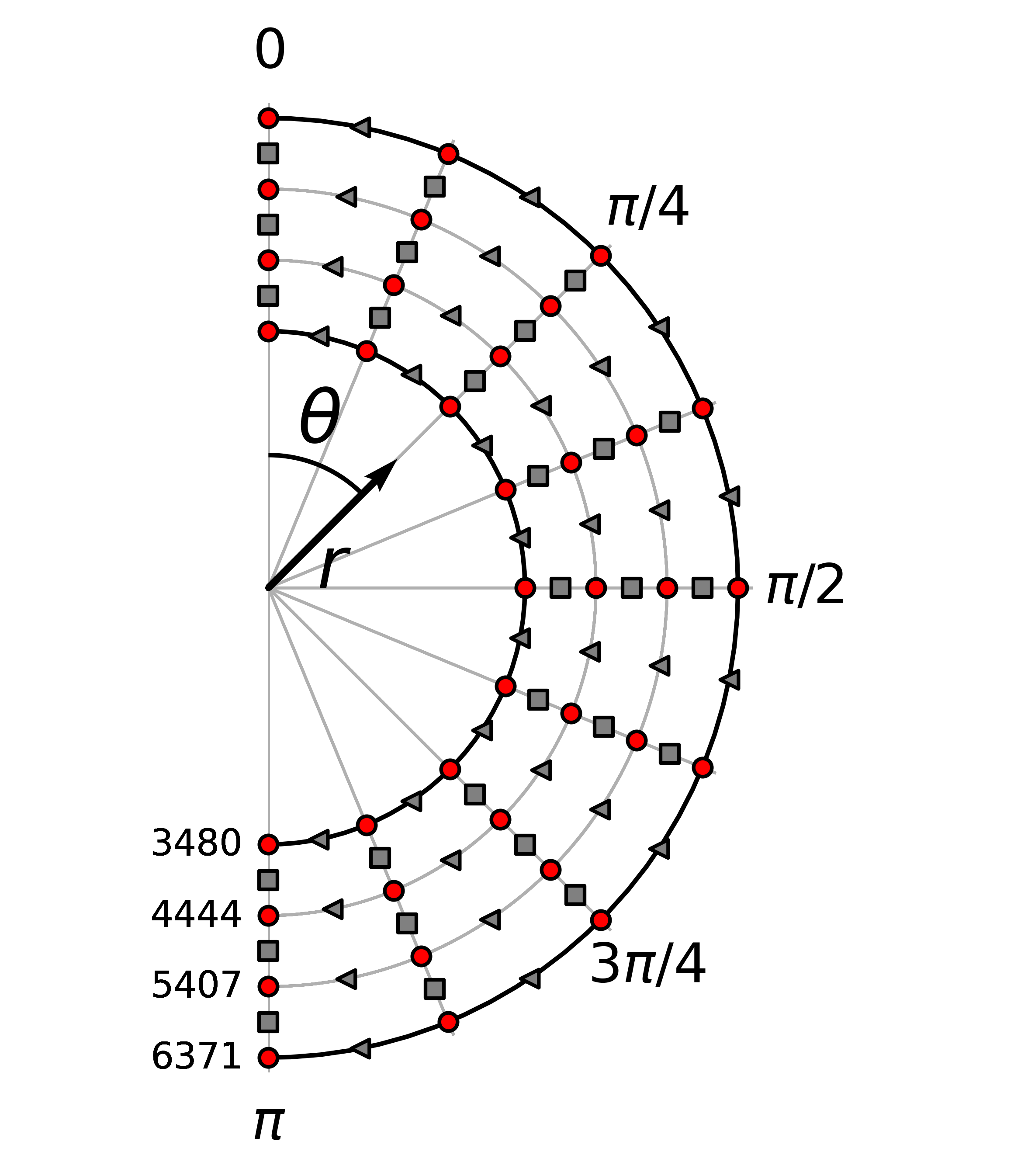
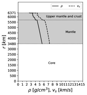
(a) (b)

Figure 3: (a): schematic of the axi-symmetric domain and staggered grid used for simulating the shear wave system in Eq.(3), where the red-filled circles represent grid points where the velocity $v$ is defined, the gray-filled squares represent those for the stress $\sigma_{r\phi}$ and the gray-filled triangles are those for the stress $\sigma_{\theta\phi}$. (b): profiles of density $\rho$ and shear velocity $v_{s}$ as a function of the radial distance down to the core-mantle boundary as defined by the PREM model. The shaded gray region represents the simulation domain.

The Rank2Galerkin formulation of the system in Eq.(3.1) can be expressed as

$$\frac{d\hat{\boldsymbol{X}}_{v}}{dt}(t;\boldsymbol{\eta},\mathcal{M}) =\hat{\mathbf{A}}_{v}(\boldsymbol{\eta})\hat{\boldsymbol{X}}_{\sigma}(t;\boldsymbol{\eta},\mathcal{M})+\boldsymbol{\Phi}_{v}^{T}\boldsymbol{F}_{v}(t;\boldsymbol{\eta},\mathcal{M})$$

(8) $$\frac{d\hat{\boldsymbol{X}}_{\sigma}}{dt}(t;\boldsymbol{\eta},\mathcal{M}) =\hat{\mathbf{A}}_{\sigma}(\boldsymbol{\eta})\hat{\boldsymbol{X}}_{v}(t;\boldsymbol{\eta},\mathcal{M}),$$

where $\hat{\mathbf{A}}_{v}(\boldsymbol{\eta})\equiv\boldsymbol{\Phi}_{v}^{T}\mathbf{A}_{v}(\boldsymbol{\eta})\boldsymbol{\Phi}_{\sigma}\in\mathbb{R}^{K_{v}\times K_{\sigma}}$ is the reduced system matrix for the velocity and $\hat{\mathbf{A}}_{\sigma}(\boldsymbol{\eta})\equiv\boldsymbol{\Phi}_{\sigma}^{T}\mathbf{A}_{\sigma}(\boldsymbol{\eta})\boldsymbol{\Phi}_{v}\in\mathbb{R}^{K_{\sigma}\times K_{v}}$ is the one for the stresses, $\boldsymbol{\Phi}_{v}$ and $\boldsymbol{\Phi}_{\sigma}$ are the orthonormal (i.e., $\boldsymbol{\Phi}_{v}^{T}\boldsymbol{\Phi}_{v}=\mathbf{I}$ and the same for $\boldsymbol{\Phi}_{\sigma}$) bases for the velocity and stresses, respectively. This enables, by default, a physics-based separation of the degrees of freedom which inherently have considerably disparate scales. This benefits the computation of the POD modes for the ROM, because they can be computed independently for velocity and stresses, and no specific scaling is required. Furthermore, it allows one to potentially use different basis sizes to represent the velocity and stresses degrees of freedom. Note that we omitted the reference state because we do not use it here. The corresponding Rank1Galerkin can be obtained by setting $M=1$.

For time integration of both the FOM and ROM, we use a leapfrog integrator, where the velocity field is updated first, followed by the stress update. This is a commonly used scheme for classical mechanics because it is time-reversible and symplectic. The initial conditions consist of zero velocity and stresses.

To the best of our knowledge, this work provides the first example of ROMs applied to elastic shear wave simulations. However, it is important to acknowledge that the application of ROMs to wave propagation is not new, and refer the reader to [55, 54]. These two studies focused on illustrating the feasibility and quantifying the accuracy of ROMs for acoustic wave simulations. Of particular interest is the discussion presented in [54] on various techniques to make ROMs feasible for three-dimensional acoustic simulations, a non-trivial task due to the size of the problem. In a future study, one could explore, for example, the combination of some of the methods presented in [55] with our rank-2 formulation.

3.2 Implementation, Material Model and Forcing

We implemented the rank-1 and rank-2 formulations of both the FOM and ROM for the shear problem above in C++ using the performance-portable Kokkos programming model [14], and make the repository publicly available at github.com/fnrizzi/ElasticShearWaves to favor scientific reproducibility and benefit other researchers. Kokkos exposes a general API allowing users to write code only once, and internally exploits compile-time polymorphism to decide on the proper data layout, and dispatching to the suitable backend depending on the target threaded system, e.g., OpenMP, CUDA, OpenCL, etc. Therefore, once the code is written, it can be easily tested on CPUs and their corresponding GPUs with minimal effort.

One of the key aspects related to modeling seismic shear waves is the choice of material model (i.e., density and shear modulus) and forcing term. Our code currently supports a few 1D material models: a single layer and a bilayer model and the Preliminary Reference Earth Model (PREM) [18]. We are in the process of adding support for the ak135f [39, 50]. We remark that these are 1D models in the sense that they only depend on the radial distance. For the single layer model, one needs to set the radial profile of the density and shear wave velocity. For the bilayer model, one needs to set the depth of the discontinuity separating the layers, and profiles within each layer. The single and bilayer models are useful for testing and exploratory cases but are obviously not fully representative of the earth structure. The PREM and ak135f are two of the most commonly used models. These models have several discontinuities and complex profiles describing the material properties . Figure 3 (b) shows the profiles of the material properties as defined by the PREM model. We designed the code in a modular fashion such that adding new material models or extending existing ones is straightforward.

The forcing term has two main defining aspects, the form of the excitation signal and the location at which it acts. We support two kinds of signals commonly used for seismic modeling, namely a Ricker wavelet and the first derivative of a Gaussian [59]. The main parameter to set for these signals is the period, $T$, which is a key property to explore for characterizing seismic events. Similar to the design of the material model, our implementation is easily extended to include other kinds of signals. As for the location, due to the axisymmetric approximation, the seismic source cannot be placed exactly on the symmetry axis [34], i.e. $\theta=0$ and $\theta=\pi$. Therefore, for a given depth, it is placed at the first velocity grid point such that $\theta>0$.

4 Results

The results presented below are obtained with a machine containing two 18-core Intel(R) Xeon(R) Gold 6154 CPU @ 3.00GHz, each with a 24.75MB L3 cache and 125GB total memory. We enable hyperthreading, thus supporting a maximum of 36 logical threads per CPU, so a total of 72 threads. We use GCC-8.3.1 and rely on kokkos and kokkos-kernels version 3.1.01. We use Blis-0.7.0 [69, 68] as the kokkos-kernels’ backend for all dense operations. In the present work we only run on CPUs enabling OpenMP as the default Kokkos execution space. A more detailed study encompassing the role of the compiler and architecture (e.g., running on GPUs) is left for a future work. The results are divided into four parts. Scaling and performance results obtained for the FOM are presented in § 4.1 and for the Galerkin ROM in § 4.2. Accuracy results and a representative use case for a many-query problem are discussed for the ROM in § 4.4 and § 4.5, respectively. For reproducibility purposes, in the supplementary material we provide the full details to access the data corresponding to the results below as well as the scripts used for the runs.

4.1 Full-order Model Performance and Scaling

In this section, we present scaling and performance tests obtained for the shear wave simulations using the Rank1FOM and Rank2FOM, see Eq.(3.1). For brevity, we omit the full details of the model and physical parameters used to carry out these FOM numerical experiments and refer the reader to supplemental material. For this analysis the physical details are not important because they only come into play during the preprocessing stage and, therefore, have no impact on the performance.

We consider $M\in\{1,2,4,8,16,32,48\}$, thread counts $2,4,8,12,18,36,72$, and total degrees of freedom $N\in\{785,152;3,143,168;12,577,792;50,321,408\}$. These values of $N$ are the total degrees of freedom originating from choosing the following grids for the velocity: $256\times 1024$, $512\times 2048$, $1024\times 4096$ and $2048\times 8192$. Note that in general one should choose the value of $M$ considering its trade off with the amount of memory required. Indeed, if one needs to save state data very frequently, using large values of $M$ can yield a very large memory utilization for the FOM problem. Here, to make this FOM analysis feasible for $M\leq 48$ and since we are not interested in the physical data, we disable all input/output related to saving data.

For the Rank2FOM, we use a row-major ordering for the state matrix. This choice, given the OpenMP execution space chosen for Kokkos, yielded a performance superior to using column-major ordering. For the sake of clarity, we remark that for the Rank1FOM we do not need to choose the memory layout, because a rank-1 state is just a 1D array. For both Rank1FOM and Rank2FOM we use the following OpenMP affinity: OMP_PLACES=threads and OMP_PROC_BIND=spread.

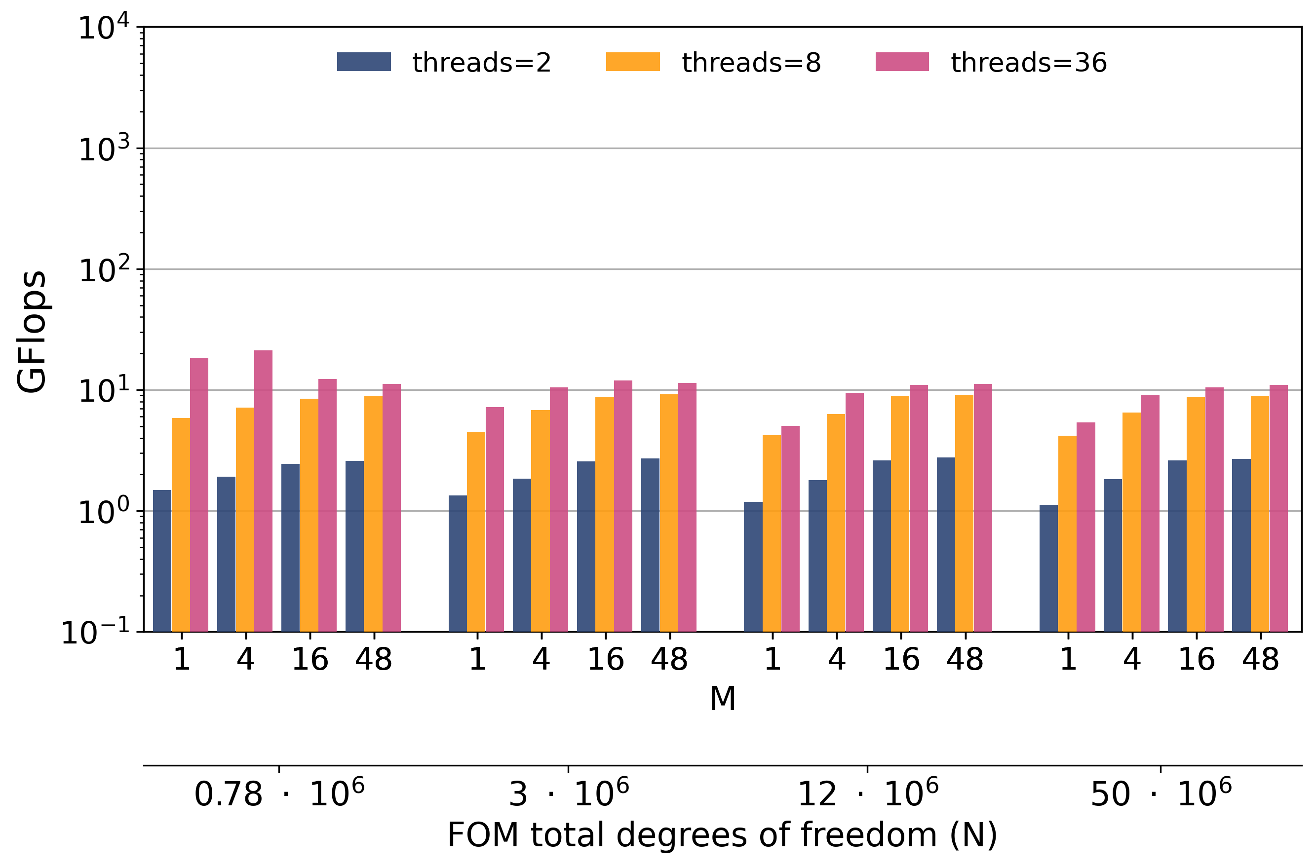
(a)
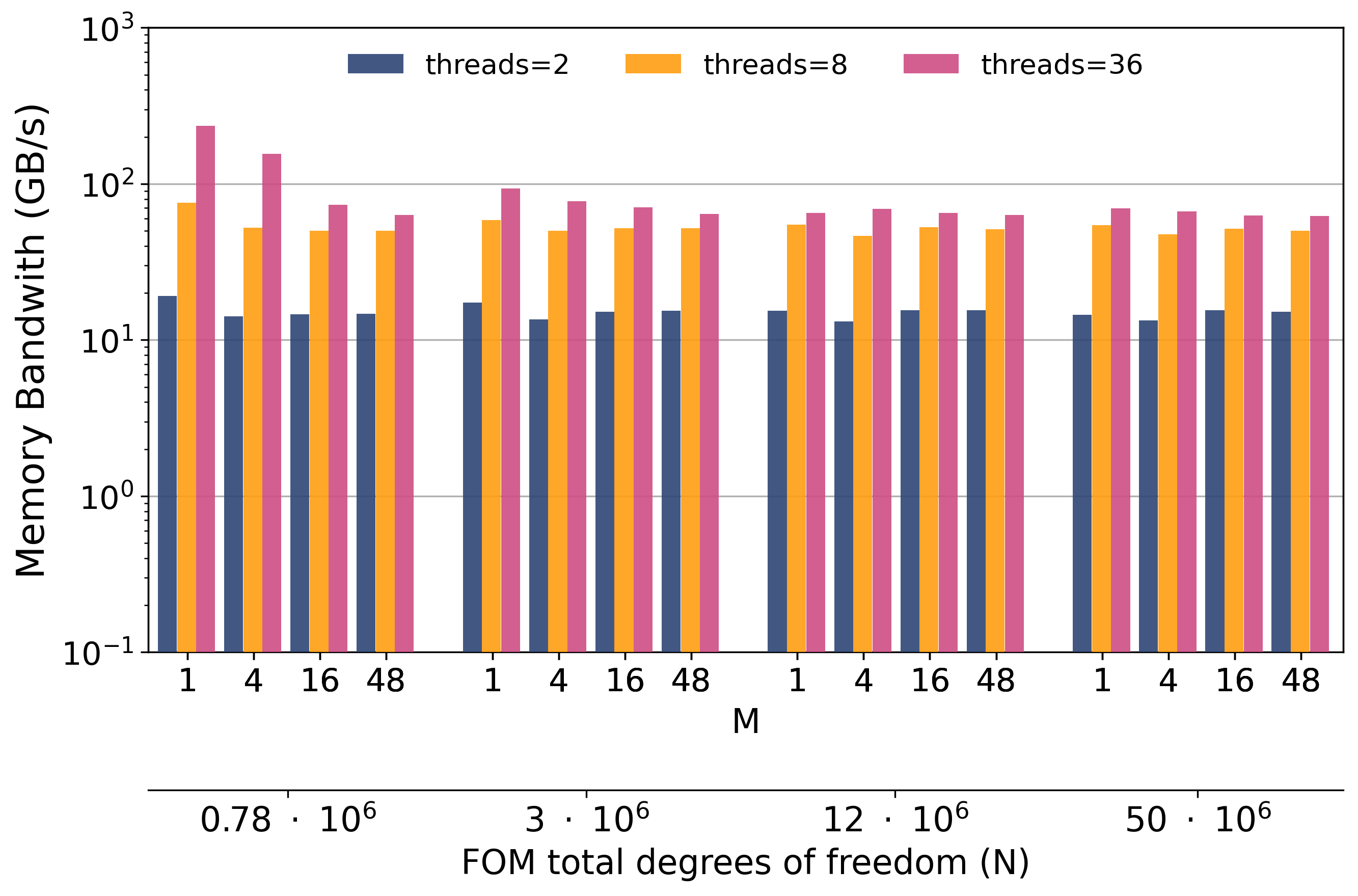
(b)
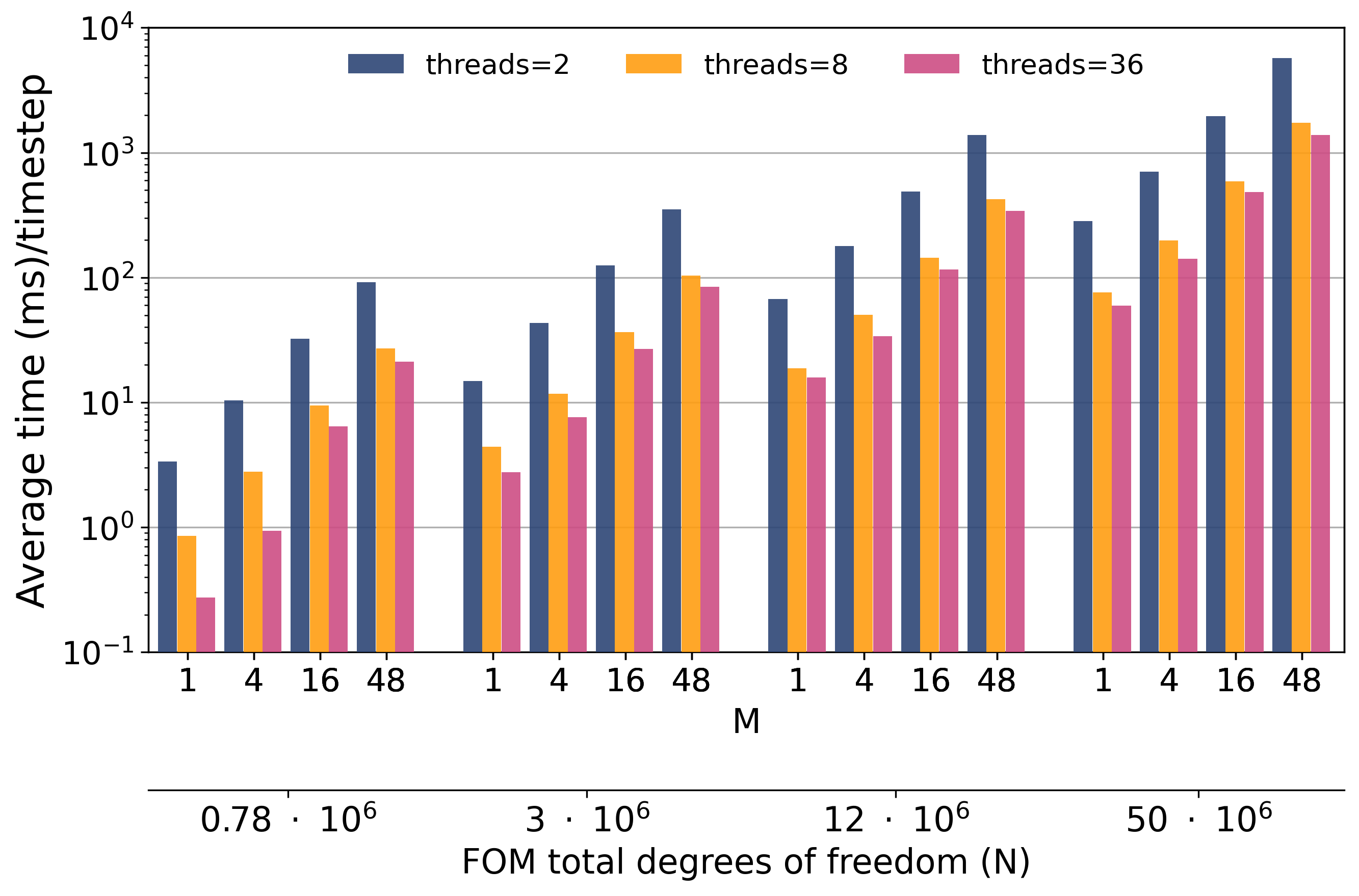
(c)

Figure 4: Performance results obtained for the full-order problem in Eq. (3.1) showing (a) the computational throughput (GFlops), (b) the memory bandwidth (GB/s), and (c) the average time (milliseconds) per time step, for various thread counts, problem and forcing sizes $M$. The limits of the vertical axes are the same as those used in Figure 5.

Figure 4 shows the computational throughput (GigaFLOPS) in panel (a), the memory bandwidth (GB/s) in panel (b) and the average time (milliseconds) per time step in panel (c) for a representative subset of values of thread counts and $M$. We make the following observations. First, Figures 4 (a,b) show that as the problem size increases and the thread count increases to $36$ the computational throughput plateaus around $10$ GFlops (which is in line with other typical sparse kernels [44]) and the memory bandwidth around about $68$ (GB/s), which is close to the max bandwidth ($\sim 85$ GB/s) of the machine in its current configuration. This indicates a good performance, and confirms that the problem is memory bandwidth bound. Second, panel (b) shows that for the smallest problem size ($N=0.78\cdot 10^{6}$), the memory bandwidth exceeds the theoretical one, indicating cache effects playing a key role at that scale. These cache effects become increasingly less evident as the problem size increases. Third, if we fix the problem size, $N$, and thread count, we observe that the performance improves if we use the rank-2 implementation. This is because of the higher arithmetic intensity of the spmm kernel in the Rank2FOM compared to spmv in the Rank1FOM. For the sake of the argument, consider the problem size $N=12\cdot 10^{6}$ and the case with $36$ threads: Figure 4 (c) shows that using $M=16$ allows us to simultaneously compute sixteen trajectories for only a seven-fold increase in the iteration time with respect to $M=1$. The plots also seem to suggest that the benefit of simulating multiple trajectories at the same time, i.e., using $M\geq 2$, is evident when going from $M=1$ to $M=4$, but then plateaus, suggesting that there is a limiting, problem-dependent value of $M$ after which no major gain is obtained. Fourth, panel (c) allows us to assess the strong scaling behavior of the FOM problem. If we fix $N$ and $M$, we observe a good scaling from 2 to 8 threads, but a degradation as we go from 8 to 36. This is expected and explained as follows: since the problem is memory bandwidth bound, and 8 threads are nearly enough for the computational kernels to saturate the memory access (see panel (b)), one cannot expect a substantial improvement in the performance if we increase the thread count.

4.2 ROM performance and scaling

This section presents scaling and performance results for the rank-1 and rank-2 Galerkin ROMs introduced in Eq.(3.1). To carry out this analysis, we make the following simplifications: (a) we use random data to fill the reduced operators in Eq.(3.1) (a demonstration and discussion of the Galerkin ROM accuracy on a real shear wave problem is presented in § 4.4 and § 4.5); (b) we turn off all input/output related to saving data and only collect timing information; and (c) we use the same ROM size, $K$, for the velocity and stresses generalized coordinates, i.e., $K_{v}=K_{\sigma}=K$.

We consider the following ROM sizes $K\in\{256,512,1024,2048,4096\}$, thread counts ${1,2,4,8,12,18,36,72}$, and $M\in\{1,2,4,8,16,32,64,128,256,512,1024\}$. Recall that the case $M=1$ corresponds to the Rank1Galerkin while $M\geq 2$ corresponds to Rank2Galerkin. We remark that these choices of $M$, despite seemingly large, are all feasible for the ROM problem thanks to the small state dimensionality. To give an example, let us consider a Galerkin ROM problem of the form Eq.(3.1) with the largest size, i.e., $K=4096$, and suppose we collect a total of $500$ reduced states. If we use $M=1000$, which corresponds to simulating $1000$ forcing realizations simultaneously, and considering we have one equation for the velocity and one for stresses, it would require only $\approx 65$ MB for the generalized coordinates, $\approx 268$ MB for the reduced system matrices and $\approx 33$ GB to store all the state snapshots. This is well within the memory capacity of modern computing nodes. Note that we are not accounting for the size of the basis because the reduced operators can all be precomputed offline.

For both Rank1Galerkin and Rank2Galerkin we use a column-major layout for all the operators; this is a suitable to interface to the BLAS library used by the kokkos-kernels to execute all the dense kernels. All runs are completed using the following OpenMP affinity: OMP_PLACES=cores and OMP_PROC_BIND=true.

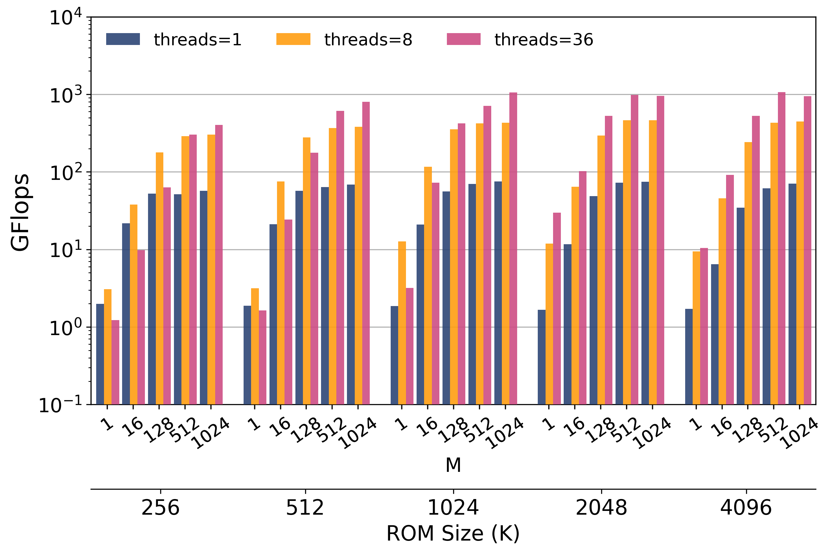
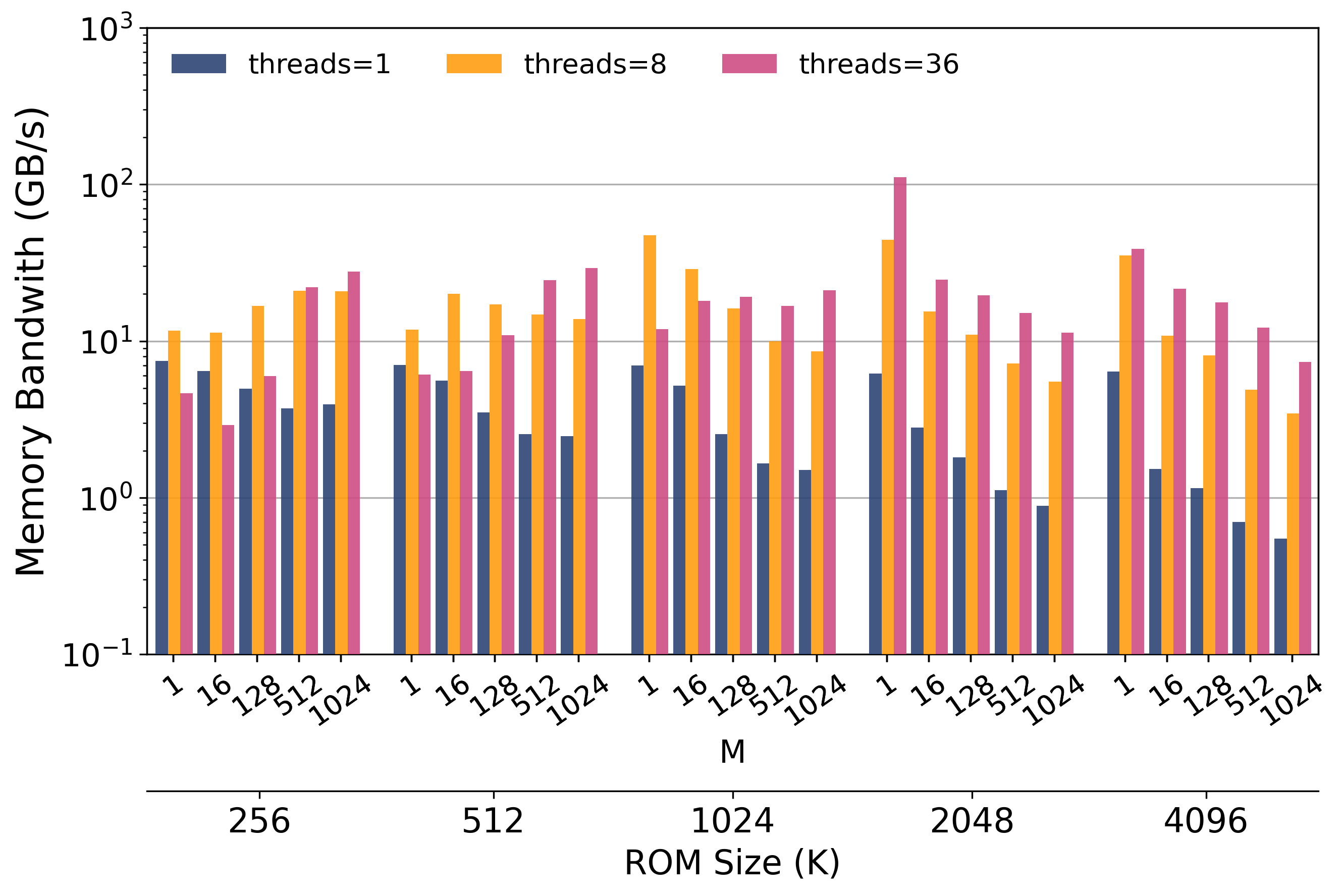
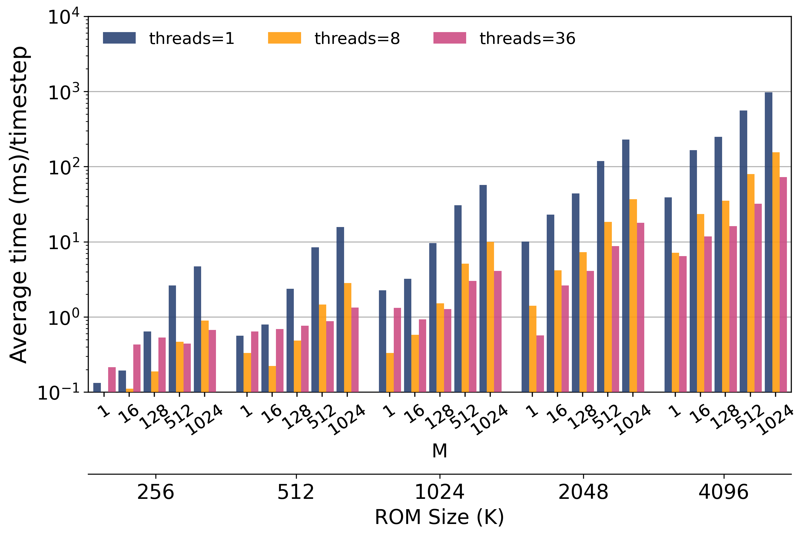
Figure 5: Performance results obtained for the ROM problem in Eq. (3.1) showing the (a) computational throughput (GFlops), (b) memory bandwidth (GB/s), and (c) average time (milliseconds) per step, for various thread counts, forcing size $M$, and number of modes $K$.

Figure 5 shows the computational throughput (GigaFLOPS) in panel (a), the memory bandwidth (GB/s) in panel (b) and the average time (milliseconds) per time step in panel (c) for a representative subset of values of threads and $M$. We make the following observations. First, Figures 5 (a,b) clearly show that Rank1Galerkin (i.e. $M=1$) is a memory bandwidth-bound problem, while Rank2Galerkin ($M>1$) is a compute-bound problem. This is evident because the case $M=1$ yields a limited throughput, namely ${\mathcal{O}(10)}$ Gflops, which remains substantially unchanged if we increase the ROM size $K$. Also, if we fix $M=1$ and increase the number of threads, we observe a minor improvement only up to 8 threads, which is already enough to saturate the system. On the contrary, when $M\geq 16$, using more threads is generally beneficial and the throughput reaches a maximum of 1TFlops when the cores are fully utilized. Compared to the GFlops obtained for $M=1$, the one for $M=16$ is one order of magnitude larger, and increases to two orders of magnitude for $M\geq 512$. Second, for the ROM sizes explored here, the computational throughput achieves its maximum when $M=512$ and no major improvement is obtained using $M=1024$. For example, for $K=2048$, using $M=512$ and 36 threads yields about 1TFlops, which remains the same for $M=1024$. Third, panel (c) allows us to assess the strong scaling behavior. We observe excellent scaling when $M\geq 16$ and the ROM size is sufficiently large, while a poor scaling is generally obtained when $M=1$, which is a direct consequence of the different nature of the kernels.

4.3 When should an analyst prefer the Rank2Galerkin?

The results above highlight the excellent performance of Rank2Galerkin and quantified the main differences between it and Rank1Galerkin. A natural question arises: when should an analyst prefer Rank2Galerkin over Rank1Galerkin? Obviously, this question only makes sense in the context of a many-query study where the interest is in simulating an ensemble of trajectories corresponding to multiple realizations of the forcing function, as in a typical forward propagation study in UQ.

Suppose we are given a target ROM size, $K$, and need to simulate an ensemble of $P$ trajectories (where $P$ is large, $P\gg 10$) from realizations of the forcing term, while needing to meet these two constraints: (a) we have a limited budget of cores available, e.g., a single node with $36$ physical cores; (b) due to, e.g., memory constraints, $1024$ is the maximum feasible number of trajectories that can simultaneously live on the node. These constraints are arbitrarily set here for the sake of the argument, but are reasonable values nonetheless. What combination of thread count, $n$, and number of simultaneous trajectories, $M$, would be the most efficient to obtain those $P$ samples while satisfying the given constraints? For example, one could launch $36$ single-threaded runs in parallel, each using $M=1$, and then repeat until all $P$ runs are completed. This implies that, at any time, all $36$ cores of the node would be occupied, and $36$ realizations of the forcing term would be running simultaneously, which means that both the core budget and the memory constraint are satisfied. A minor variation would be to run $18$ two-threaded runs at the same time each using $M=1$. This would still satisfy both the core budget and the memory constraint. The most interesting scenarios arise when we vary $M$. Generalizing, this is a (discrete) constrained optimization problem, since we need to optimize over number of threads and $M$. Solving this in a general context is outside the scope of this work, but we provide the following insights.

Let $\tau(K,n,M)$ represent the runtime to complete a single Galerkin ROM simulation of the form Eq.(3.1) with ROM size $K_{v}=K_{\sigma}=K$, using $n$ threads and a given value $M$. It follows that the total runtime to complete trajectories for $P$ forcing realizations with a budget of $36$ threads can be expressed as

(9) $$\tau^{P}(K,n,M)=\tau(K,n,M)\frac{P}{\frac{36}{n}M},$$

because $\frac{36}{n}$ is the number of independent runs executing in parallel on the node with each run responsible of computing $M$ trajectories. We can define the following metric

(10) $$s(K,n,M)=\frac{\tau^{P}(K,1,1)}{\tau^{P}(K,n,M)}=\frac{\tau(K,1,1)}{\tau(K,n,M)}\frac{M}{n},$$

where $s(K,n,M)>1$ indicates Rank2Galerkin is more efficient than Rank1Galerkin, while the opposite is true for $s(K,n,M)<1$. This metric can be interpreted as a speedup (or slowdown) factor.

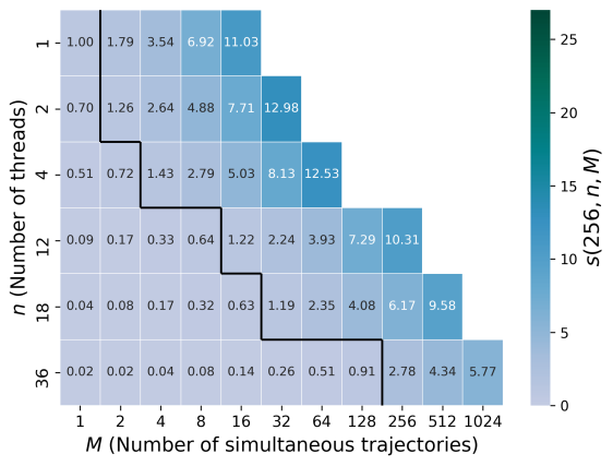
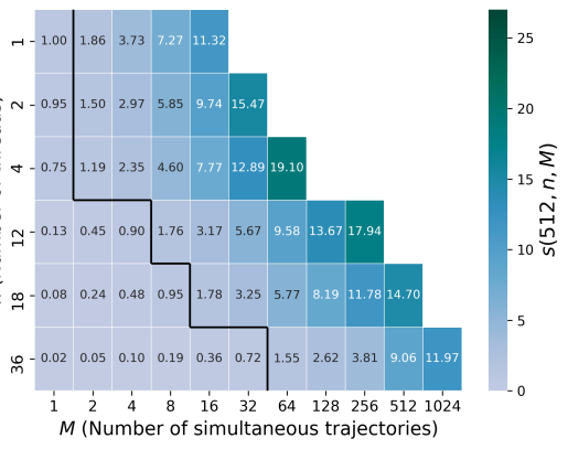
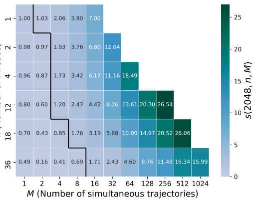
(a) (b)
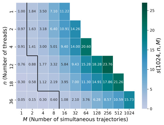
(c) (d) . On each plot, the solid black line separates the cases where $s(K,n,M)>1$ (i.e., where Rank2Galerkin is more convenient) from those where $s(K,n,M)<1$ (i.e., where Rank1Galerkin is more convenient). The white region in each plot identifies the non-admissible cases, i.e., combinations violating the constraints listed in § 4.3.

Figure 6: Heatmap visualization of $s(K,n,M)$ (see Eq. 10) computed for ROM sizes ${K=256}$ (a), $512$ (b), $1024$ (c) and $2048$ (d), and various values of $M$ and $n$

Figure 6 shows a heatmap visualization of $s(K,n,M)$ computed for various values of $M$ and $n$, and ROM sizes $K\in\{256,512,1024,2048\}$. To generate these plots, we used the runtimes obtained in § 4.2. The plots allow us to reason about what is the most efficient setting. For example, looking at Figure 6 (a), which corresponds to $K=256$, we observe that using Rank2Galerkin with $M=32$ and $n=2$ yields $s(256,2,32)=12.98$, which means that for this setup the Rank2Galerkin is about $13$ times more efficient than using Rank1Galerkin with $n=1$. Depending on the given ROM size, similar conclusions can be made. The second key observation is that as the ROM size increases, it becomes increasingly more convenient to rely on Rank2Galerkin. For example, if we fix $n=12$ and $M=256$, we see that when $K=256$ we have a 10X speedup with respect to Rank1Galerkin with $n=1$ (see Figure 6 (a)), but we reach a 26X speedup for $K=2048$, see Figure 6 (d).

The above results suggest that, if the goal is to compute an ensemble of trajectories for different realizations of the forcing term and the main cost function is the runtime, Rank2Galerkin should always be preferred over the Rank1Galerkin.

4.4 Predictive and reproductive ROM accuracy

We now discuss the accuracy of the Galerkin ROM for the elastic shear wave test case under consideration. We consider the scenario where the period, $T$, parameterizing the forcing signal varies over a fixed interval, $T\in[31,69]$, and aim to quantify how accurately the Galerkin ROM can approximate the FOM predictions as $T$ varies over that interval. Note that since here the focus is on quantifying the accuracy, it does not matter which ROM formulation is used. We use Rank2Galerkin to perform the analysis because it is more efficient, but the same results would be obtained using Rank1Galerkin.

The complete definition of the problem is as follows. We use the PREM as material model, a total simulation time of $t_{final}=2000$ (seconds) and a time step size $\Delta t=0.1$ (seconds) to ensure stability. The forcing acts at $150$ (km) depth, and is modeled as a Ricker wavelet with $90$ seconds delay and period $T$. This delay, combined with the total integration time, represents a system that is at rest for a small period of time, and then excites and decays due to the action of the forcing. For the FOM runs, we use the grid with $N=3,143,168$ total degrees of freedom, which we recall stems from using a $512\times 2048$ velocity grid. This grid is chosen because, given $T=31$ and the PREM material model, it is the smallest one (in powers of two) satisfying the numerical dispersion criterion we use in our code.

To compute the POD modes for the ROM, we proceed as follows: we run the FOM at $T=35,65$, save the velocity and stress states every $2$ seconds, and then merge the data from both training points into a single snapshot matrix which is used to compute the POD modes via SVD. We deliberately choose only two training points for two main reasons: (a) it is the smallest training set one can choose to sample a one-dimensional parameter space; and (b) it mimics a realistic situation where limited data are available. This occurs, for example, when a computational model is very expensive to run such that an analyst can only afford a few runs, or where experimental data is collected at just a few parameter points and more experiments are not affordable. For such cases, in fact, relying on data-driven models requiring large training datasets is unfeasible. We thus believe it is interesting to assess whether one can construct a sufficiently accurate ROM given limited data, which, if positive, would highlight the full power of ROMs versus purely data-driven models.

Our goal is to characterize both a reproductive and predictive scenario. A reproductive scenario occurs when the ROM accuracy is quantified and evaluated at the same (training) points in the parameter space used to generate the basis functions of the ROM. In this case, this means evaluating the ROM accuracy for $T\in\{35,65\}$. A predictive scenario is where the ROM accuracy is evaluated at parameter instances (test points) that differ from those used to generate the basis functions of the ROM. Here, the predictive analysis is run at $10$ random samples over the parameter range $(35,65)$, as well as $T=31$ and $T=69$, outside the training range. We remark that this is a key choice because it allows us to assess the extrapolation capabilities of the ROM, which generally is one of the main weaknesses of purely data-driven methods.

To quantify the accuracy of the ROM, we rely on the following relative error

(11) $$E_{\ell_{2}}=\frac{{\left\lVert\boldsymbol{x}(t_{final};\boldsymbol{\eta},\boldsymbol{\mu})-\tilde{\boldsymbol{x}}(t_{final};\boldsymbol{\eta},\boldsymbol{\mu})\right\rVert}_{2}}{{\left\lVert\boldsymbol{x}(t_{final};\boldsymbol{\eta},\boldsymbol{\mu})\right\rVert}_{2}}$$

where $\boldsymbol{x}(t_{final};\boldsymbol{\eta},\boldsymbol{\mu})$ is the FOM state (for either velocity or stresses) computed at the final time $t_{final}$ for the given parameters $\boldsymbol{\eta},\boldsymbol{\mu}$, and $\tilde{\boldsymbol{x}}(t_{final};\boldsymbol{\eta},\boldsymbol{\mu})$ is the state field reconstructed from the ROM results. Relying on the final time is sufficient for the purposes of this section, and in § 4.5 we show some results quantifying the error over the full simulation time.

Figure 7 (a) shows the relative error (11) computed for the velocity degrees of freedom as a function of the period $T$. The results are shown for $(K_{v},K_{\sigma})\in\{(311,276),(369,343),(415,394),(436,417)\}$, which corresponds to truncating $10^{-5}$, $10^{-7}$, $10^{-9}$ and $10^{-10}$ of the POD cumulative energy, respectively. To compute the cumulative energy, we use the same fomula defined in [66]).

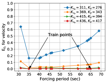
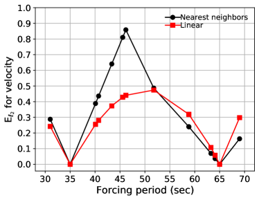
(a) (b)
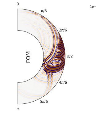
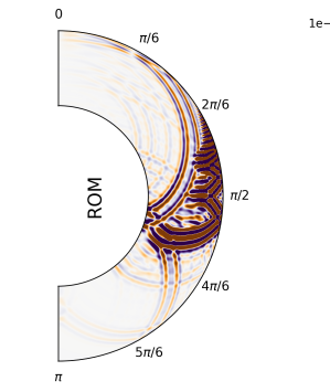
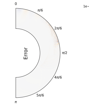
(c)

Figure 7: Panel (a) shows the relative error, see Eq.(11), computed for the velocity degrees of freedom between the FOM solution and the corresponding ROM-based approximation as a function of the period $T$ and for various ROM sizes $K$. Panel (b) shows the same relative error metric computed between the FOM and the state approximation obtained via nearest neighbor and linear interpolation using the FOM state at $T=35$ and $T=65$ as training points. Panel (c) shows the velocity wave field computed with the FOM (left), the ROM with $(436,417)$ modes (middle), as well as their error field (right) at $t_{final}=2000$ (seconds) for the extrapolation point $T=69$.

As expected, increasing the ROM size increases the accuracy. We observe that to obtain errors smaller than $5\%$ within the training interval one would need to use at least $(K_{v},K_{\sigma})=(369,343)$, but that this choice would still yield a large error of about $12\%$ at the extrapolation point $T=31$. To have small errors both within the training interval and in the extrapolation regime, one would need at least $(K_{v},K_{\sigma})=(415,394)$. If a sufficient number of modes is chosen, the accuracy of the ROM is excellent across the full range and also at the extrapolation points. Similar error results are obtained for the stresses but we omit the corresponding plot for brevity. We remark that we purposefully omit the data obtained for lower energies because those cases yield unacceptable results reaching relative errors that are above 100 % for some values of $T$. For this application, the convective nature of the problem can force the need for a large number of modes to accurately predict the dynamics. However, this is not a weakness but can be an advantage in this case because, as discussed in § 4.2, the compute-bound kernels involved in Rank2Galerkin become more efficient and scalable as $K$ increases (up to value which is typically large, ${\mathcal{O}(10000)}$).

For the sake of argument, Figure 7 (b) shows the same relative error metric computed between the FOM and the state obtained via nearest-neighbor and linear interpolation using the FOM states at $T=35$ and $T=65$ to compute the approximation. A linear interpolation is the best we can do with two data points. Figure 7 (b) shows that both nearest-neighbor and linear interpolation have quite poor accuracy overall, with errors reaching up to $90\%$ inside the training range and consistently larger than $15\%$ at the extrapolation points. This indicates that, for this test case, the ROM is much more robust and accurate than interpolation.

Panel (c) shows a contour plot of the wave field at the final time $t_{final}=2000$ (seconds) for the source signal period $T=69$ (recall that this is an extrapolation point) computed with the FOM (left), ROM with ${(K_{v},K_{\sigma})=(436,417)}$ (middle), and their error field (right). We observe very little difference between the FOM and ROM results, mostly near the earth surface in the range $2\pi/6<\theta<\pi/2$.

Given the scope of this work, the above discussion was limited to a representative analysis, but we anticipate a full comparison between the FOM, ROM and other surrogate models (e.g., polynomials or neural nets) to be an interesting study to perform. Several questions arise:

• How many more training points would one need to use for a polynomial approximation to match the ROM accuracy?

• What is the best performing surrogate when the number of training points is larger than two?

• What is the trade off between the cost of computing the surrogate and its accuracy?

• How would the results change if one considered a higher-dimensional parameter space?

4.5 Many-query scenario

We conclude the results demonstrating the application of Rank2Galerkin to a many-query analysis. Using the same problem definition described in § 4.4, we assume the period, $T$, parameterizing the forcing signal is uncertain and follows a uniform distribution ${\mathcal{U}}(31,69)$. We aim to quantify how this parametric uncertainty impacts the model predictions. This is a typical forward UQ study, which we approach using Monte Carlo sampling.

We use the Rank2FOM and Rank2Galerkin to perform $P=512$ realizations of $T$ by randomly sampling ${\mathcal{U}}(31,69)$. For the ROM runs, we use $K_{v}=436$ and $K_{\sigma}=417$ (since these values proved to be accurate, see Figure 7(a)), and select the most efficient combination of threads and $M$ by leveraging the performance results shown in § 4.2. Based on Figure 6 (b) (since $K=512$ is a good approximation of $K_{v}$ and $K_{\sigma}$ used here), we choose $M=64$ and $n=4$ threads to run each Rank2Galerkin simulation. For the FOM, we use four threads $n=4$ and $M=4$ for each run. This choice is made by using the FOM results in § 4.1 to compute a metric similar to the one computed for the ROM in § 4.3, and extracting the most efficient combination. This is reported in § SM2 of the supplemental material.

4.5.1 Accuracy

Figure 8 shows the seismograms—and representative statistics computed using the ensemble of 512 runs—collected at locations on the earth surface, $r=6371$ km, with polar angles $\theta=10^{\circ}$ and $60^{\circ}$. The left column of Figure 8 shows the mean and the 5-95th percentile bounds over the full time domain computed with the ROM using $K_{v}=436$ and $K_{\sigma}=417$. The right column of Figure 8 shows magnified views of specific time windows displaying curves for different percentiles as well as the mean and error bars computed with the FOM. The predictions are characterized by substantial variations, stemming from the complex pattern of reflections, refractions and interference of the shear waves through the domain, and the ROM accurately approximates the FOM results over the full time domain in both its mean trend and statistics. Note that in this case, the inherently complex dynamics of the waves prevents one from being able to characterize the wavefield variability just by evaluating the extreme values of the forcing period $T$. It is therefore critical to sample the full range of $T$ to obtain accurate statistics, which are fundamental to potentially assess risk and extreme events probabilities.

Figure 8: Seismograms with representative statistics obtained at receivers on the earth surface, $r=6371$ km, with polar angles $\theta=10^{\circ}$ (first row), $60^{\circ}$ (second row), computed from the UQ analysis described in § 4.5.

4.5.2 Computational Gain

To quantify the computational gain, we can reason as follows.
Rank2Galerkin. Since we rely on a computing node with $36$ physical cores, and use Rank2Galerkin with four threads and $M=64$, we can launch 8 such simulations in parallel to compute $8\times 64=512$ trajectories. These 8 runs execute in parallel, and therefore finish in approximately the same time as a single run with four threads and $M=64$, which is about $7.5$ seconds for the current problem on the machine we used.
Rank2FOM. For the FOM, we use individual runs with four threads and $M=4$, implying that we can evaluate 8 runs in parallel, and complete the full ensemble of $P$ trajectories with 16 sets of runs. Each run takes about $455$ seconds, so the total runtime is approximately $455\times 16=7280$ seconds. For the current problem and setup, Rank2Galerkin is thus about $970$ times faster than the FOM.

If we were to run the same analysis using the Rank1Galerkin, we would launch 36 parallel single-threaded runs with $M=1$, thus needing about $14$ sets of such runs to complete the full ensemble of $P$ trajectories. The approximate runtime of one such Rank1Galerkin is about $8$ seconds, so the total runtime is approximately $8\times 14=112$ seconds. Rank2Galerkin is $15$ times faster than Rank1Galerkin.

Here we are not accounting for the cost of computing the basis for the ROM simulations for two main reasons: first, computing the POD basis only needs to be done once during the offline stage; second, computing the POD for a very tall skinny matrix (i.e., $m_{r}\gg m_{c}$ where $m_{r}$ and $m_{c}$ are the number of rows and columns, respectively) can be efficiently done leveraging one of the algorithms scaling with $m_{c}$, see, e.g., chapter 45 in [28].

We can summarize the following benefits in using the Galerkin ROM for this seismic application: first, if needed, we can query the system very efficiently for either a single or several values of $T$ to explore different statistics; second, the dimensionality of the ROM is small enough such that one can store the full time evolution of the generalized coordinates and use them later on to efficiently reconstruct the full wave fields at target times; third, computing the seismograms from the ROM data can be done very efficiently because we can just use individual rows of the POD basis to reconstruct the field at target points on the earth surface thus avoiding the need to load the full basis matrix in memory.

5 Conclusions

We presented a reformulation, called rank-2 Galerkin, of the Galerkin ROM for LTI dynamical systems to convert them from memory bandwidth- to compute-bound problems. We described the details of the formulation and highlighted its benefits compared to the formulation adopted so far in the community. Rank-2 Galerkin is suitable to solve many-query problems driven by the forcing term in a scalable and efficient way on modern computing node architectures.

We demonstrated the rank-2 Galerkin using, as a test case, the simulation of elastic seismic shear waves in an axisymmetric domain. We showed the excellent scalability of rank-2 Galerkin with respect to the number of cores, which is a result of the nature of the underlying computational kernels. We quantified the accuracy of the ROM for this application as the period of the forcing varies, and showed that for this problem, a Galerkin ROM has excellent accuracy in both the reproductive and predictive scenarios. Using a Monte Carlo sampling exercise, we demonstrated the quantification of the uncertainty in the wavefields stemming from a uncertain forcing period, and showed that rank-2 Galerkin is about $970$ times faster than the FOM while being extremely accurate in both the mean and statistics of the field.

As alluded to in this manuscript, several interesting future directions and applications arise. In addition to problems of the form (1), the rank-2 formulation may yield computational gains in other ROM contexts, e.g., linearized systems (sensitivity and stability analysis), gradient-based solvers for nonlinear ROMs, and nonlinear ROMs with polynomial nonlinearities [38].

The approach could be generalized to the case where the state and forcing are rank-3 tensors. This would enable one to simultaneously compute multiple realizations of $\boldsymbol{\eta}$ (which parametrizes the system matrix) and $\boldsymbol{\mu}$ (which parametrizes the forcing only). In this case, an obstacle to overcome would be to efficiently assemble the reduced system matrices for multiple realizations of $\boldsymbol{\eta}$. The feasibility of this strictly depends on the parameterization of the system matrix: if the parameters can be decoupled from the matrix, then the reduced system matrices may be computed efficiently; if this decoupling is not possible, one could leverage interpolation methods applied to the system matrix [4]. This rank-3 formulation would open up interesting opportunities from a computational standpoint, for example employing higher-order singular value decompositions [2] and drawing ideas from the advances on tensor algebra taking place within the deep learning community, where rank-3 tensors are at the core of formulations. Of particular interest are algorithmic developments for batched matrix multiplication kernels [63, 1, 45, 35] and hardware innovations such as tensor cores [48] and tensor processing units [37].

Beyond linear problems, one could assess the feasibility of applying a reformulation similar to the one presented here to ROMs of nonlinear systems, and the potential gains of applying the rank-2 or rank-3 Galerkin ROMs to inverse problems in geophysics. Another critical aspect is the practical challenge related to implementing rank-2 Galerkin in a performance-portable way as a library to be used by other applications. The latter topic is of particular interest to us: we are currently working on the design and implementation of the rank-2 Galerkin formulation in our ROM library Pressio.

Appendix A Problem setup for the FOM scaling results

To run the FOM scaling tests presented in § 4.1, we employ a material model comprising a single, homogeneous layer with $\rho=2500$ (g/cm³) and ${v_{s}=5000}$ (m/s). The source signal acts at $640$ (km) of depth and takes the form of the first derivative of a Gaussian. For the Rank1FOM, the source has a period $T=60$ (seconds) and delay $180$ (seconds), while for the Rank2FOM each forcing term has the same Gaussian form but with a period randomly sampled over the interval (60, 80). The numerical dispersion condition is satisfied for all problems sizes. The time step size is $\Delta t=0.05$ such that numerical stability is ensured for all problem sizes considered, and each run completes $1000$ time steps, which allows us to collect meaningful timing statistics of the computational kernels.

Appendix B When should an analyst prefer the Rank2FOM?

In this section, we present for the FOM an analysis similar to the one done for the ROM in § 4.3. Here, we set the constraints as follows. First, we assume a limited budget of cores available, e.g., a single node with $36$ physical cores. Second, we constrain the maximum number of forcing values running simultaneously on the node to be $48$. This can stem from, e.g., memory constraints. Note that unlike the Rank2Galerkin, the Rank2FOM cannot have too many simultaneous forcing terms being evaluated at the same time on the node because the memory requirements are much bigger. Therefore, this poses a much stricter limit, and we arbitrarily choose $48$ as a constraint for the sake of the argument noting, however, that it is quite a large value.

Similarly to § 4.3, we proceed as follows. Let $\tau(N,n,M)$ represent the runtime to complete a single FOM simulation of the form Eq.(3.2) with $N$ total degrees of freedom using $n$ threads and a given value $M$. It follows that the total runtime to complete trajectories for $P$ forcing realizations with a budget of $36$ threads can be expressed as

(12) $$\tau^{P}(N,n,M)=\tau(N,n,M)\frac{P}{\frac{36}{n}M},$$

because $\frac{36}{n}$ is the number of independent runs executing in parallel on the node with each run responsible of computing $M$ trajectories. We can define the following metric

(13) $$s(N,n,M)=\frac{\tau^{P}(N,2,1)}{\tau^{P}(N,n,M)}=\frac{\tau(N,2,1)}{\tau(N,n,M)}\frac{2M}{n},$$

where $s(N,n,M)>1$ indicates Rank2FOM is more efficient than Rank1FOM, while the opposite is true for $s(N,n,M)<1$. We remark that the reference case used here for this metric is the Rank1FOM using $n=2$ threads, since for the FOM we never use less than $2$ threads, see § 4.1.

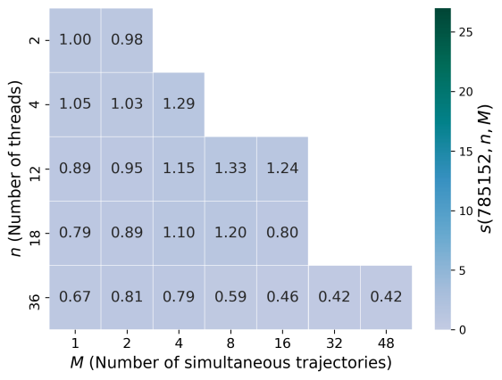
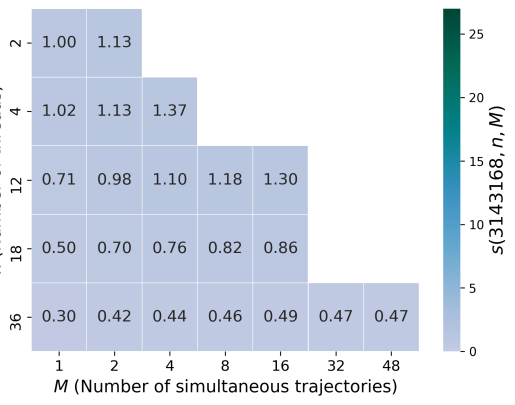
(a) (b)
(c) (d)

Figure 9: Heatmap visualization of $s(N,n,M)$ (see Eq. 13) computed for $N=785,152$ (a), $3,143,168$ (b), $12,577,792$ (c) and $50,321,408$ (c), and various values of $M$ and $n$. The white region in each plot identifies the cases violating the constraints listed in § B. Note that we set the colorbar with the same limits used in § 4.3 to facilitate the comparison between the two sets of results.

Figure 9 shows a heatmap visualization of $s(N,n,M)$ computed for various values of $M$ and $n$, and $N\in\{785,152;3,143,168;12,577,792;50,321,408\}$. To generate these plots, we used the FOM runtimes obtained in § 4.1. The heatmap plot allows us to reason as follows. For example, for the $3\cdot 10^{6}$ problem size, using $M=4$ and $n=4$ is $37\%$ more efficient than the case $M=1,n=2$, and becomes $59\%$ more efficient if we consider the $50\cdot 10^{6}$ problem size. For $M=16$ and $n=12$, the gain is about $30\%$ for the $3\cdot 10^{6}$ case and becomes $43\%$ for the $50\cdot 10^{6}$ one. This trend suggests that the gain increases with the problem size. It is interesting to note that the gains are overall quite small, never exceeding $60\%$. This is due to the fact that while the Rank2FOM has a higher compute intensity than Rank1FOM, they are both memory-bandwidth bound problems, and therefore they are both limited. This is in contrast to what we observed for the ROM in § 4.3, where we obtained up to 26 times speedup using the rank-2 ROM formulation.

Appendix C Data and Code Availability

The code developed for this work and data used in the paper are publicly available at:

• Code repository:   https://github.com/fnrizzi/ElasticShearWaves
  Git hash: 2e4cf2151d3e284b4ce3c29f7f6a12efa097915b

• The full dataset:   https://github.com/fnrizzi/RomLTIData contains the data as well as the scripts to generate the plots

References

- [1] A. Abdelfattah, A. Haidar, S. Tomov, and J. Dongarra, Performance, design, and autotuning of batched GEMM for GPUs, in High Performance Computing, J. M. Kunkel, P. Balaji, and J. Dongarra, eds., Cham, 2016, Springer International Publishing, pp. 21–38, https://doi.org/10.1007/978-3-319-41321-1_2.
- [2] S. Afra and E. Gildin, Tensor based geology preserving reservoir parameterization with higher order singular value decomposition (hosvd), Computers & Geosciences, 94 (2016), pp. 110–120, https://doi.org/10.1016/j.cageo.2016.05.010.
- [3] K. Ahmad, A. Venkat, and M. Hall, Optimizing LOBPCG: Sparse matrix loop and data transformations in action, in Languages and Compilers for Parallel Computing, C. Ding, J. Criswell, and P. Wu, eds., Cham, 2017, Springer International Publishing, pp. 218–232, https://doi.org/10.1007/978-3-319-52709-3_17.
- [4] D. Amsallem, R. Tezaur, and C. Farhat, Real-time solution of linear computational problems using databases of parametric reduced-order models with arbitrary underlying meshes, Journal of Computational Physics, 326 (2016), pp. 373–397, https://doi.org/10.1016/j.jcp.2016.08.025.
- [5] S. Banerjee, A. Mukhopadhyay, S. Sen, and R. Ganguly, Thermomagnetic convection in square and shallow enclosures for electronics cooling, Numerical Heat Transfer, Part A: Applications, 55 (2009), pp. 931–951, https://doi.org/10.1080/10407780902925440.
- [6] U. Baur, P. Benner, and L. Feng, Model order reduction for linear and nonlinear systems: A system-theoretic perspective, Archives of Computational Methods in Engineering, 21 (2014), pp. 331–358, https://doi.org/10.1007/s11831-014-9111-2.
- [7] Y. Bazilevs, M.-C. Hsu, and M. Scott, Isogeometric fluid–structure interaction analysis with emphasis on non-matching discretizations, and with application to wind turbines, Computer Methods in Applied Mechanics and Engineering, 249 (2012), pp. 28–41, https://doi.org/10.1016/j.cma.2012.03.028.
- [8] N. Bell and M. Garland, Efficient sparse matrix-vector multiplication on CUDA, NVIDIA Technical Report NVR-2008-004, NVIDIA Corporation, Dec. 2008, https://www.nvidia.com/docs/IO/66889/nvr-2008-004.pdf.
- [9] P. Benner, S. Gugercin, and K. Willcox, A survey of projection-based model reduction methods for parametric dynamical systems, SIAM Review, 57 (2015), pp. 483–531, https://doi.org/10.1137/130932715.
- [10] P. Benner, J. Saak, and M. M. Uddin, Structure preserving model order reduction of large sparse second-order index-1 systems and application to a mechatronics model, Mathematical and Computer Modelling of Dynamical Systems, 22 (2016), pp. 509–523, https://doi.org/10.1080/13873954.2016.1218347, https://doi.org/10.1080/13873954.2016.1218347, https://arxiv.org/abs/https://doi.org/10.1080/13873954.2016.1218347.
- [11] G. Berkooz, P. Holmes, and J. L. Lumley, The proper orthogonal decomposition in the analysis of turbulent flows, Annual Review of Fluid Mechanics, 25 (1993), pp. 539–575, https://doi.org/10.1146/annurev.fl.25.010193.002543.
- [12] M. Borg and M. Collu, Frequency-domain characteristics of aerodynamic loads of offshore floating vertical axis wind turbines, Applied energy, 155 (2015), pp. 629–636, https://doi.org/10.1016/j.apenergy.2015.06.038.
- [13] T. Bui-Thanh, K. Willcox, and O. Ghattas, Parametric reduced-order models for probabilistic analysis of unsteady aerodynamic applications, AIAA Journal, 46 (2008), pp. 2520–2529, https://doi.org/10.2514/1.35850.
- [14] H. Carter Edwards, C. R. Trott, and D. Sunderland, Kokkos, J. Parallel Distrib. Comput., 74 (2014), pp. 3202–3216, https://doi.org/10.1016/j.jpdc.2014.07.003.
- [15] E. Chaljub and A. Tarantola, Sensitivity of ss precursors to topography on the upper-mantle 660-km discontinuity, Geophysical Research Letters, 24 (1997), pp. 2613–2616, https://doi.org/10.1029/97GL52693.
- [16] P. Chetty, Current injected equivalent circuit approach to modeling of switching dc-dc converters in discontinuous inductor conduction mode, IEEE Transactions on industrial electronics, (1982), pp. 230–234, https://doi.org/10.1109/TIE.1982.356670.
- [17] E. Dowell, A Modern Course in Aeroelasticity, Solid Mechanics and its Applcations, Springer International Publishing, 2015, https://doi.org/10.1007/978-3-319-09453-3.
- [18] A. M. Dziewonski and D. L. Anderson, Preliminary reference Earth model, Physics of the Earth and Planetary Interiors, 25 (1981), pp. 297 – 356, https://doi.org/10.1016/0031-9201(81)90046-7.
- [19] A. Elafrou, G. Goumas, and N. Koziris, Performance analysis and optimization of sparse matrix-vector multiplication on Intel Xeon Phi, in 2017 IEEE International Parallel and Distributed Processing Symposium Workshops (IPDPSW), 2017, pp. 1389–1398, https://doi.org/10.1109/IPDPSW.2017.134.
- [20] J. Epting, Thermal management of urban subsurface resources - delineation of boundary conditions, Procedia Engineering, 209 (2017), pp. 83–91, https://doi.org/https://doi.org/10.1016/j.proeng.2017.11.133. The Urban Subsurface - from Geoscience and Engineering to Spatial Planning and Management.
- [21] J. E. Ffowcs Williams and D. L. Hawkings, Sound generation by turbulence and surfaces in arbitrary motion, Philosophical Transactions of the Royal Society of London. Series A, Mathematical and Physical Sciences, 264 (1969), p. 321–342, https://doi.org/10.1098/rsta.1969.0031.
- [22] M. Goman and A. Khrabrov, State-space representation of aerodynamic characteristics of an aircraft at high angles of attack, Journal of Aircraft, 31 (1994), pp. 1109–1115, https://doi.org/10.1007/978-3-319-09453-3.
- [23] Grepl, Martin A. and Patera, Anthony T., A posteriori error bounds for reduced-basis approximations of parametrized parabolic partial differential equations, ESAIM: M2AN, 39 (2005), pp. 157–181, https://doi.org/10.1051/m2an:2005006.
- [24] S. Gugercin, A. Antoulas, and C. Beattie, model reduction for large-scale linear dynamical systems, SIAM Journal on Matrix Analysis and Applications, 30 (2008), pp. 609–638, https://doi.org/10.1137/060666123.
- [25] S. Gugercin and A. C. Antoulas, A survey of model reduction by balanced truncation and some new results, International Journal of Control, 77 (2004), pp. 748–766, https://doi.org/10.1080/00207170410001713448, https://doi.org/10.1080/00207170410001713448, https://arxiv.org/abs/https://doi.org/10.1080/00207170410001713448.
- [26] M. Gunzburger, N. Jiang, and M. Schneier, An ensemble-proper orthogonal decomposition method for the nonstationary navier–stokes equations, SIAM J. Numer. Anal., 55 (2017), p. 286–304, https://doi.org/10.1137/16M1056444.
- [27] M. Gunzburger, N. Jiang, and Z. Wang, An efficient algorithm for simulating ensembles of parameterized flow problems, IMA Journal of Numerical Analysis, 39 (2018), pp. 1180–1205, https://doi.org/10.1093/imanum/dry029.
- [28] L. Hogben, ed., Handbook of Linear Algebra, CRC Press, Boca Raton, FL, USA, 2006.
- [29] C. Hong, A. Sukumaran-Rajam, B. Bandyopadhyay, J. Kim, S. E. Kurt, I. Nisa, S. Sabhlok, U. V. Çatalyürek, S. Parthasarathy, and P. Sadayappan, Efficient sparse-matrix multi-vector product on GPUs, in Proceedings of the 27th International Symposium on High-Performance Parallel and Distributed Computing, HPDC ’18, New York, NY, USA, 2018, Association for Computing Machinery, p. 66–79, https://doi.org/10.1145/3208040.3208062.
- [30] A. Hutcheson and V. Natoli, Memory bound vs. compute bound: A quantitative study of cache and memory bandwidth in high performance applications, 2011, http://docplayer.net/33565764-Memory-bound-vs-compute-bound-a-quantitative-study-of-cache-and-memory-bandwidth-in-high-performance-applications.html.
- [31] D. Hyland and D. Bernstein, The optimal projection equations for model reduction and the relationships among the methods of Wilson, Skelton, and Moore, IEEE Transactions on Automatic Control, 30 (1985), pp. 1201–1211, https://doi.org/10.1109/TAC.1985.1103865.
- [32] H. Igel and M. Weber, SH-wave propagation in the whole mantle using high-order finite differences, Geophysical Research Letters, 22 (1995), pp. 731–734, https://doi.org/https://doi.org/10.1029/95GL00312.
- [33] F. P. Incropera, A. S. Lavine, T. L. Bergman, and D. P. DeWitt, Fundamentals of heat and mass transfer, Wiley, 2007.
- [34] G. Jahnke, M. S. Thorne, A. Cochard, and H. Igel, Global SH-wave propagation using a parallel axisymmetric spherical finite-difference scheme: Application to whole mantle scattering, Geophysical Journal International, 173 (2008), pp. 815–826, https://doi.org/10.1111/j.1365-246X.2008.03744.x.
- [35] L. Jiang, C. Yang, and W. Ma, Enabling highly efficient batched matrix multiplications on SW26010 many-core processor, ACM Trans. Archit. Code Optim., 17 (2020), https://doi.org/10.1145/3378176.
- [36] N. Jiang and W. Layton, An algorithm for fast calculation of flow ensembles, International Journal for Uncertainty Quantification, 4 (2014), pp. 273–301, https://doi.org/10.1615/Int.J.UncertaintyQuantification.2014007691.
- [37] N. P. Jouppi, C. Young, N. Patil, D. Patterson, G. Agrawal, R. Bajwa, S. Bates, S. Bhatia, N. Boden, A. Borchers, R. Boyle, P.-l. Cantin, C. Chao, C. Clark, J. Coriell, M. Daley, M. Dau, J. Dean, B. Gelb, T. V. Ghaemmaghami, R. Gottipati, W. Gulland, R. Hagmann, C. R. Ho, D. Hogberg, J. Hu, R. Hundt, D. Hurt, J. Ibarz, A. Jaffey, A. Jaworski, A. Kaplan, H. Khaitan, D. Killebrew, A. Koch, N. Kumar, S. Lacy, J. Laudon, J. Law, D. Le, C. Leary, Z. Liu, K. Lucke, A. Lundin, G. MacKean, A. Maggiore, M. Mahony, K. Miller, R. Nagarajan, R. Narayanaswami, R. Ni, K. Nix, T. Norrie, M. Omernick, N. Penukonda, A. Phelps, J. Ross, M. Ross, A. Salek, E. Samadiani, C. Severn, G. Sizikov, M. Snelham, J. Souter, D. Steinberg, A. Swing, M. Tan, G. Thorson, B. Tian, H. Toma, E. Tuttle, V. Vasudevan, R. Walter, W. Wang, E. Wilcox, and D. H. Yoon, In-datacenter performance analysis of a tensor processing unit, in Proceedings of the 44th Annual International Symposium on Computer Architecture, ISCA ’17, New York, NY, USA, 2017, Association for Computing Machinery, p. 1–12, https://doi.org/10.1145/3079856.3080246.
- [38] I. Kalashnikova, S. Arunajatesan, M. F. Barone, B. G. van Bloemen Waanders, and J. A. Fike, Reduced order modeling for prediction and control of large-scale systems., (2014), https://doi.org/10.2172/1177206.
- [39] B. L. N. Kennett, E. R. Engdahl, and R. Buland, Constraints on seismic velocities in the Earth from traveltimes, Geophysical Journal International, 122 (1995), pp. 108–124, https://doi.org/10.1111/j.1365-246X.1995.tb03540.x.
- [40] K. Kunisch and S. Volkwein, Galerkin proper orthogonal decomposition methods for parabolic problems, Numerische Mathematik, 90 (2001), pp. 117–148, https://doi.org/10.1007/s002110100282.
- [41] S. Lall, P. Krysl, and J. E. Marsden, Structure-preserving model reduction for mechanical systems, Physica D: Nonlinear Phenomena, 184 (2003), pp. 304 – 318, https://doi.org/https://doi.org/10.1016/S0167-2789(03)00227-6, http://www.sciencedirect.com/science/article/pii/S0167278903002276. Complexity and Nonlinearity in Physical Systems – A Special Issue to Honor Alan Newell.
- [42] S. Lall, J. E. Marsden, and S. Glavaški, Empirical model reduction of controlled nonlinear systems, IFAC Proceedings Volumes, 32 (1999), pp. 2598–2603, https://doi.org/10.1016/S1474-6670(17)56442-3. 14th IFAC World Congress 1999, Beijing, Chia, 5-9 July.
- [43] E. E. Lewis and W. F. Miller, Computational methods of neutron transport, (1984), https://www.osti.gov/biblio/5538794.
- [44] A. Li, R. S. Hammad Mazhar, and D. Negrut, Comparison of SPMV performance on matrices with different matrix format using CUSP, cuSPARSE and ViennaCL, (2015), https://sbel.wiscweb.wisc.edu/wp-content/uploads/sites/569/2018/05/TR-2015-02.pdf.
- [45] X. Li, Y. Liang, S. Yan, L. Jia, and Y. Li, A coordinated tiling and batching framework for efficient GEMM on GPUs, in Proceedings of the 24th Symposium on Principles and Practice of Parallel Programming, PPoPP ’19, New York, NY, USA, 2019, Association for Computing Machinery, p. 229–241, https://doi.org/10.1145/3293883.3295734.
- [46] M. J. Lighthill, On sound generated aerodynamically i. general theory, Proceedings of the Royal Society of London. Series A. Mathematical, Physical, and Engineering Sciences Physical Sciences, 211 (1952), p. 564–587, https://doi.org/10.1098/rspa.1952.0060.
- [47] O. Lombard, C. Barrière, and V. Leroy, Nonlinear multiple scattering of acoustic waves by a layer of bubbles, EPL (Europhysics Letters), 112 (2015), p. 24002, https://doi.org/10.1209/0295-5075/112/24002.
- [48] S. Markidis, S. W. D. Chien, E. Laure, I. B. Peng, and J. S. Vetter, Nvidia tensor core programmability, performance precision, in 2018 IEEE International Parallel and Distributed Processing Symposium Workshops (IPDPSW), 2018, pp. 522–531, https://doi.org/10.1109/IPDPSW.2018.00091.
- [49] L. Meirovitch, Fundamentals of vibrations, Waveland Press, 2010.
- [50] J.-P. Montagner and B. L. N. Kennett, How to reconcile body-wave and normal-mode reference Earth models, Geophysical Journal International, 125 (1996), pp. 229–248, https://doi.org/10.1111/j.1365-246X.1996.tb06548.x.
- [51] B. Moore, Principal component analysis in linear systems: Controllability, observability, and model reduction, IEEE Transactions on Automatic Control, 26 (1981), pp. 17–32, https://doi.org/10.1109/TAC.1981.1102568.
- [52] C. T. Mullis and R. A. Roberts, Synthesis of minimum roundoff noise fixed point digital filters, IEEE Transactions on Circuits and Systems, 23 (1976), pp. 551–562, https://doi.org/10.1109/TCS.1976.1084254.
- [53] E. Peise, Performance modeling and prediction for dense linear algebra, 2017, https://arxiv.org/abs/1706.01341.
- [54] V. Pereyra, Model order reduction with oblique projections for large scale wave propagation, Journal of Computational and Applied Mathematics, 295 (2016), pp. 103 – 114, https://doi.org/https://doi.org/10.1016/j.cam.2015.01.029. VIII Pan-American Workshop in Applied and Computational Mathematics.
- [55] V. Pereyra and A. Kaelin, Fast wave propagation by model order reduction, Electronic Transactions on Numerical Analysis. Volume, 30 (2008), pp. 406–419, http://emis.impa.br/EMIS/journals/ETNA/vol.30.2008/pp406-419.dir/pp406-419.pdf.
- [56] O. M. Phillips, On the generation of sound by supersonic turbulent shear layers, Journal of Fluid Mechanics, 9 (1960), pp. 1–28, https://doi.org/10.1017/S0022112060000888.
- [57] E. Phipps, M. D’Elia, H. C. Edwards, M. Hoemmen, J. Hu, and S. Rajamanickam, Embedded ensemble propagation for improving performance, portability and scalability of uncertainty quantification on emerging computational architectures, 2015, https://arxiv.org/abs/1511.03703.
- [58] C. Prud’Homme, D. Rovas, K. Veroy, L. Machiels, Y. Maday, A. Patera, and G. Turinici, Reliable Real-Time Solution of Parametrized Partial Differential Equations: Reduced-Basis Output Bound Methods, J. of Fluids Eng., 124 (2001), pp. 70–80, https://doi.org/10.1137/130932715.
- [59] E. V. Rabinovich, N. Y. Filipenko, and G. S. Shefel, Generalized model of seismic pulse, Journal of Physics: Conference Series, 1015 (2018), p. 052025, https://doi.org/10.1088/1742-6596/1015/5/052025.
- [60] D. Rovas, L. Machiels, and Y. Maday, Reduced-basis output bound methods for parabolic problems, IMA Journal of Numerical Analysis, 26 (2006), https://doi.org/10.1093/imanum/dri044.
- [61] D. V. Rovas, Reduced-basis output bound methods for parametrized partial differential equations, PhD thesis, Massachusetts Institute of Technology, 2003, http://hdl.handle.net/1721.1/16956.
- [62] R. K. Shah and D. P. Sekulic, Fundamentals of heat exchanger design, John Wiley & Sons, 2003.
- [63] Y. Shi, U. N. Niranjan, A. Anandkumar, and C. Cecka, Tensor contractions with extended blas kernels on cpu and gpu, in 2016 IEEE 23rd International Conference on High Performance Computing (HiPC), 2016, pp. 193–202, https://doi.org/10.1109/HiPC.2016.031.
- [64] J. R. Singler, New pod error expressions, error bounds, and asymptotic results for reduced order models of parabolic pdes, SIAM Journal on Numerical Analysis, 52 (2014), pp. 852–876, https://doi.org/10.1137/120886947.
- [65] L. Sirovich, Turbulence and the dynamics of coherent structures part i: Coherent structures, Quarterly of Applied Mathematics, 45 (1987), pp. 561–571, http://www.jstor.org/stable/43637457.
- [66] R. Swischuk, B. Kramer, C. Huang, and K. Willcox, Learning Physics-Based Reduced-Order Models for a Single-Injector Combustion Process, AIAA Journal, 58 (2020), pp. 2658–2672, https://doi.org/10.2514/1.J058943.
- [67] J. Tencer, K. Carlberg, M. Larsen, and R. Hogan, Accelerated solution of discrete ordinates approximation to the boltzmann transport equation for a gray absorbing–emitting medium via model reduction, Journal of Heat Transfer, 139 (2017), https://doi.org/10.1115/1.4037098.
- [68] F. G. Van Zee, T. Smith, F. D. Igual, M. Smelyanskiy, X. Zhang, M. Kistler, V. Austel, J. Gunnels, T. M. Low, B. Marker, L. Killough, and R. A. van de Geijn, The BLIS framework: Experiments in portability, ACM Transactions on Mathematical Software, 42 (2016), pp. 12:1–12:19, https://doi.org/10.1145/2755561.
- [69] F. G. Van Zee and R. A. van de Geijn, BLIS: A framework for rapidly instantiating BLAS functionality, ACM Transactions on Mathematical Software, 41 (2015), pp. 14:1–14:33, https://doi.org/10.1145/2764454.
- [70] J. Virieux, SH-wave propagation in heterogeneous media: velocity-stress finite-difference method, Exploration Geophysics, 15 (1984), pp. 265–265, https://doi.org/10.1071/EG984265a.
- [71] J. Virieux, P-SV wave propagation in heterogeneous media: Velocity‐stress finite‐difference method, GEOPHYSICS, 51 (1986), pp. 889–901, https://doi.org/10.1190/1.1442147.
- [72] J. Vlach, V. Jiří, and K. Singhal, Computer methods for circuit analysis and design, Springer Science & Business Media, 1983.
- [73] S. Volkwein, Model reduction using proper orthogonal decomposition, 2011. lecture notes, university of konstanz, www.math.uni-konstanz.de/numerik/ personen/volkwein/teaching/pod-vorlesung.pdf. reduction for parametrized pdes 27 andrea manzoni cmcs – modelling and scie, in CMCS – Modelling and Scientific Computing MATHICSE – Mathematics Institute of Computational Science and Engineering EPFL – Ecole Polytechnique Fédérale de Lausanne Station 8, CH-1015 Lausanne Switzerland and MOX – Modellistica e Calcolo Scientifico Dipart, 2012.
- [74] Y. Wang, H. Takenaka, X. Jiang, and J. Lei, Modelling two-dimensional global seismic wave propagation in a laterally heterogeneous whole-Moon model, Geophysical Journal International, 192 (2012), pp. 1271–1287, https://doi.org/10.1093/gji/ggs094.
- [75] K. Willcox and J. Peraire, Balanced model reduction via the proper orthogonal decomposition, AIAA Journal, 40 (2002), pp. 2323–2330, https://doi.org/10.2514/2.1570.
- [76] D. A. Wilson, Optimum solution of model-reduction problem, Proceedings of the Institution of Electrical Engineers, 117 (1970), pp. 1161–1165, https://doi.org/10.1137/130932715.
- [77] H. Yang and M. Gunzburger, Algorithms and analyses for stochastic optimization for turbofan noise reduction using parallel reduced-order modeling, Computer Methods in Applied Mechanics and Engineering, 319 (2017), pp. 217 – 239, https://doi.org/10.1016/j.cma.2017.02.030.
- [78] D. Yuen, J. Wang, L. Johnsson, C.-H. Chi, and Y. Shi, GPU Solutions to Multi-Scale Problems in Science and Engineering, Springer Publishing Company, Inc., 1st ed., 2011, https://doi.org/10.1007/978-3-642-16405-7.
- [79] C. Zhao and T. Lu, Analysis of microchannel heat sinks for electronics cooling, International Journal of Heat and Mass Transfer, 45 (2002), pp. 4857–4869, https://doi.org/10.1016/S0017-9310(02)00180-1.
- [80] Zhaoqing Chen, Linear circuit model combination for coupled noise simulation by using directional junction, in IEEE 14th Topical Meeting on Electrical Performance of Electronic Packaging, 2005., 2005, pp. 83–86, https://doi.org/10.1109/EPEP.2005.1563707.