An Introduction to the Deviatoric Tensor Decomposition in Three Dimensions and its Multipole Representation

Abstract

The analysis and visualization of tensor fields is a very challenging task. Besides the cases of zeroth- and first-order tensors, most techniques focus on symmetric second-order tensors. Only a few works concern totally symmetric tensors of higher-order. Work on other tensors of higher-order than two is exceptionally rare. We believe that one major reason for this gap is the lack of knowledge about suitable tensor decompositions for the general higher-order tensors. We focus here on three dimensions as most applications are concerned with three-dimensional space. A lot of work on symmetric second-order tensors uses the spectral decomposition. The work on totally symmetric higher-order tensors deals frequently with a decomposition based on spherical harmonics. These decompositions do not directly apply to general tensors of higher-order in three dimensions. However, another option available is the deviatoric decomposition for such tensors, splitting them into deviators. Together with the multipole representation of deviators, it allows to describe any tensor in three dimensions uniquely by a set of directions and non-negative scalars. The specific appeal of this methodology is its general applicability, opening up a potentially general route to tensor interpretation. The underlying concepts, however, are not broadly understood in the engineering community. In this article, we therefore gather information about this decomposition from a range of literature sources. The goal is to collect and prepare the material for further analysis and give other researchers the chance to work in this direction. This article wants to stimulate the use of this decomposition and the search for interpretation of this unique algebraic property. A first step in this direction is given by a detailed analysis of the multipole representation of symmetric second-order three-dimensional tensors.

Keywords Tensor  $\cdot$ Higher-order  $\cdot$ Deviatoric Decomposition  $\cdot$ Multipole Decomposition  $\cdot$ Stiffness Tensor

1 Introduction

Analysis and visualization of tensor fields focuses mainly on symmetric second-order fields like mechanical stress and strain. There is also work on general second-order tensor fields like the velocity gradient in fluid flow. But there are many more tensor fields used in natural sciences and engineering to describe the behaviour of matter and various fields. However, there is only very limited work on their analysis and visualization. In the life sciences, there is some work on the analysis and visualization of higher-order tensors, especially higher-order diffusion tensors. However, these tensors are totally symmetric and of even-order. If this property does not hold, literature gets exceptionally sparse.

A look at most of this work [1, 2, 3, 4] reveals that analysis and visualization of symmetric tensor fields nearly always uses the eigendecomposition, i.e. eigenvalues and eigenvectors. For general tensors of second-order, authors split them into the asymmetric part which is interpreted as vector or rotation and a symmetric part which again is analyzed using eigenvalues and eigenvectors most often. The work on totally symmetric tensors of higher even order uses a decomposition based on spherical harmonics in most cases. Unfortunately, these decompositions do not work for general tensors of higher order in three dimensions. We therefore suspect that the lack of work on the analysis and visualization of other tensors is caused by missing knowledge on tensor decompositions of these tensors.

The good news is that there is such a decomposition, namely the deviatoric decomposition, allowing to split each tensor in three dimensions into a set of deviators, i.e. traceless totally symmetric tensors. Furthermore, these deviators can be uniquely represented by a finite set of directions and a non-negative scalar. The generality of this methods renders it quite appealing for study in tensor analysis and visualization. Because this decomposition is not very well established and has gone largely unnoticed in the applied sciences, this work gives an overview of the so called deviatoric decomposition. The deviatoric decomposition is an orthogonal decomposition of a tensor of arbitrary-order up to dimension three. The deviatoric decomposition of a second-order tensor is well known. It is given by the tensor’s symmetric part and a vector, representing its asymmetric part. These deviators again can be represented by the symmetrization of a tensor product of first-order tensors (vectors) which are called multipoles. The deviatoric decomposition and the multipole representation are unique, so each tensor can be represented by a unique set of first-order tensors, i.e. vectors.

The underlying calculations go back to Maxwell [5] and were summarized by Backus [6] who also provided further information and some mathematical background. Zou et al. [7] gave explicit formulae to calculate the multipoles of a tensor.

The goal of this article is to give a summary of the multipole decomposition to enable further analysis of this representation. Until now, the meaning of the individual deviators is, to the best of our knowledge, not known for cases higher than order two. This paper should enable the analysis of higher-order tensors using the deviatoric decomposition within a single framework. To gain a first impression we analyze the second-order multipole decomposition for symmetric tensors in more detail and discuss a connection between the multipoles and the eigenvectors.

The paper is organized in the following way. First, a general introduction to the required tensor algebra is given. Then, the mathematical background of the deviatoric decomposition and the multipole representation is presented. Because of their prevalence and familiarity, the second- and fourth-order decompositions are described in more detail to explain the calculations. The final chapter describes a more or less well known application of the multipole decomposition: The multipoles of a stiffness tensor can be used to calculate the anisotropy type of the underlying material. However, as stated earlier, the exact meaning of the various deviators is, to the best of our knowledge, not known. In further works we want to change this. Identifying the meaning of such abstract object requires interpretations from a range of different fields which can all contribute unique insights. Therefore, we want to provide other researchers with the necessary tools and concepts to analyze the meaning of the deviators. Furthermore, we hope to find more applications for the deviatoric decomposition and the multipole representation to learn more about their potential meaning in the light of their generality.

2 Tensor algebra

The reader may consider the dimension $n$ to be three in most cases. To ease the description without loss of generality, we will assume an orthonormal basis at all times, so there will be no distinction between co- and contravariant tensors and all indices will be lower indices.

We denote the $n$-dimensional Euclidean vector space as $\mathcal{V}_{n}$. Its scalar product is a bilinear mapping of two vectors $\textbf{x},\textbf{y}$ to a real number and is denoted as $\textbf{x}\cdot\textbf{y}$. We assume that we are given an orthonormal basis $\{\textbf{e}_{1},\ldots,\textbf{e}_{n}\}$, i.e. $\textbf{e}_{i}\cdot\textbf{e}_{j}=\delta_{ij}$ with the Kronecker delta $\delta_{ij}$. Because no distinction between co- and contravariant tensors is required, we define an $n$-dimensional tensor of order $q$ as multilinear map of $q$ vectors to the real numbers

$$\mathds{T}:(\mathcal{V}_{n})^{q}\to\mathds{R}\text{.}$$ (1)

As a multilinear map, the tensor can also be described by its coefficients with respect to a fixed orthonormal basis of $\mathcal{V}_{n}$, say $\{\textbf{e}_{i}\}$

$$\mathds{T}(\textbf{e}_{i_{1}},\ldots,\textbf{e}_{i_{q}})=T_{i_{1},\ldots,i_{q}}$$ (2)

Therefore, a zeroth-order tensor can be represented as a scalar, a first-order tensor as a vector of dimension $n$ and a second-order tensor as an $n\times n$-matrix. Higher-order tensors can be represented as arrays of order $q$. For example, the coefficients of a three-dimensional fourth-order tensor can be represented as $3\times 3\times 3\times 3$ array. In some cases, the tensors in this paper will be described by this index notation. Then the number of the indices describes the order of the tensor. If there is another orthonormal basis $\{\textbf{f}_{1},\ldots,\textbf{f}_{n}\}$ of $\mathcal{V}_{n}$ expressed in the basis $\{\textbf{e}_{i}\}$ as $\textbf{f}_{j}=\sum_{i=1}^{n}c_{ij}\textbf{e}_{i}$ then $\mathds{T}$ is represented by the numbers

$$T^{\prime}_{j_{1}j_{2}\ldots j_{q}}=\sum_{i_{1}=1}^{n}\ldots\sum_{i_{q}=1}^{n}c_{i_{1}j_{1}}\ldots c_{i_{q}j_{q}}T_{i_{1}\ldots i_{q}}$$ (3)

with respect to the basis $\{\textbf{f}_{j}\}$. In the following, we describe our tensors always as coefficient arrays of order $q$, i.e. as represented with respect to the basis $\{\mathbf{e}_{i}\}$. This is also the representation in our (and probably any typical) visualization application.

Let $\mathds{S},\mathds{T}$ be tensors of order $q$ over $\mathcal{V}_{n}$, and $a,b\in\mathds{R}$. Then, the set of all $q$-arrays, with the scalar multiplication and the tensor addition

$$a\mathds{S}+b\mathds{T}=aS_{i_{1}i_{2}\dots i_{q}}+bT_{i_{1}i_{2}\dots i_{q}}$$ (4)

create a $n^{q}$-dimensional vector space $\mathcal{V}_{n}^{q}$ representing all $n$-dimensional tensors of order $q$.

An often used tensor operation is the tensor product or outer product. The tensor product of a $q$th-order tensor $\mathds{A}$ and a $r$th-order tensor $\mathds{B}$ results in a $(q+r)$th-order tensor $\mathds{C}$ as follows

$$\mathds{C}_{i_{1}\dots i_{q}j_{1}\dots j_{r}}=\mathds{A}\otimes\mathds{B}=A_{i_{1}\dots i_{q}}B_{j_{1}\dots j_{r}}$$ (5)

Mathematically, this creates an algebra of all tensors of arbitrary order over $\mathcal{V}_{n}$.

Another tensor operation we use is called tensor contraction. The tensor contraction is the summation over a determined number of indices. The single contraction $\mathds{C}=\mathds{A}\cdot\mathds{B}$ is the summation of two tensors $\mathds{A}$ and $\mathds{B}$ over one index

$$\begin{split}C_{i_{1}i_{2}\dots i_{n-1}j_{2}\dots j_{m}}&=\mathds{A}\cdot\mathds{B}=\sum\limits_{k=1}^{n}A_{i_{1}i_{2}\dots i_{n-1}k}B_{kj_{2}\dots j_{m}}\\ &=A_{i_{1}i_{2}\dots i_{n-1}k}B_{kj_{2}\dots j_{m}}\end{split}$$ (6)

where the implicit summation over a repeated index, i.e. $A_{i_{1}i_{2}\dots i_{n-1}k}B_{kj_{2}\dots j_{m}}$, is called Einstein summation convention. The double contraction $\mathds{A}:\mathds{B}$ is analogously defined as

$$\begin{split}C_{i_{1}i_{2}\dots i_{n-2}j_{3}\dots j_{m}}&=\mathds{A}:\mathds{B}=\sum\limits_{k=1}^{n}\sum\limits_{l=1}^{n}A_{i_{1}i_{2}\dots i_{n-2}kl}B_{klj_{3}\dots j_{m}}\\ &=A_{i_{1}i_{2}\dots i_{n-2}kl}B_{klj_{3}\dots j_{m}}\end{split}$$ (7)

One can define a trace $\text{tr}_{i,j}$ for each index pair $i,j$, but here we will define the general trace $\text{tr}()$ of a tensor as the following sum about the first two indices

$$\text{tr }(\textbf{T})=\text{tr}_{1,2}(\textbf{T})=\sum\limits_{s=1}^{n}D_{ssi_{3}i_{4}\dots i_{n}}$$ (8)

which generalizes the notion well-known for second-order tensors. Therefore, a tensor of order higher than two has more than one trace. The determinant of a second-order tensor T is defined as

$$\det(\textbf{T})\quad=\quad T_{11}T_{22}T_{33}+T_{12}T_{23}T_{13}+T_{13}T_{12}T_{23}$$ (9)

$$-T_{13}^{2}T_{22}-T_{23}^{2}T_{11}-T_{12}^{2}T_{33}$$

Let $\mathcal{S}_{q}$ be the $q$^th-order symmetric group of all $q!$ permutations $\pi$ on the integers $(1,2,\dots,q)$. Let $\mathds{T}$ be a three-dimensional tensor of order $q$. Then the permutation of the tensor $\pi\mathds{T}$ can be defined as

$$(\pi\mathds{T})_{i_{\pi_{1}}\dots i_{\pi_{q}}}=T_{i_{1}\dots i_{q}}$$ (10)

We call a tensor $\mathds{T}$ totally symmetric if $\pi\mathds{T}=\mathds{T}$ for all $\pi\in\mathcal{S}_{q}$. So, every symmetric second-order tensor is totally symmetric. A tensor of order $2n$ can have the so called minor symmetry, which means it is invariant to index permutations in the sets $\{1,2\}$ and $\{2n-1,2n\}$ of index positions. These even-order tensors can also have the major symmetry, which describes the invariance of a permutation of the index positions $\{1,\dots,n\}$ with $\{n+1,\dots,2n\}$. For a fourth-order three-dimensional tensor $\mathds{T}$ the minor symmetries and the major symmetry are given by

$$T_{ijkl}=T_{jikl}=T_{ijlk},\qquad T_{ijkl}=T_{klij}.$$ (11)

It is important for the following discussion that total symmetry implies more symmetry than minor and major symmetries alone. This becomes clear if one realizes that a totally symmetric three-dimensional fourth-order tensor has $15$ independent coefficients, i.e. $\dim(\mathcal{S}^{4})=15$. In contrast, a three-dimensional fourth-order tensor with minor and major symmetries has $21$ independent coefficients. Based on these definitions, we define the totally symmetric part $\textbf{s}\mathds{T}$ of a general tensor as

$$\textbf{s}\mathds{T}=\frac{1}{q!}\sum\limits_{\pi\in\mathcal{S}_{q}}\pi\mathds{T}$$ (12)

We call the remainder

$$\textbf{a}\mathds{T}=\mathds{T}-\textbf{s}\mathds{T}$$ (13)

the asymmetric part of $\mathds{T}$. Obviously, the asymmetric part of any tensor has no totally symmetric part which creates a vector space of all asymmetric tensors which is actually orthogonal to the totally symmetric tensor space, see [6]. The symmetric and traceless part of a tensor $\mathds{T}$ will be described by $\lfloor\mathds{T}\rfloor$. For the tensor product $\textbf{n}\otimes\textbf{m}$ it is

$$\lfloor\textbf{n}\otimes\textbf{m}\rfloor=\frac{1}{2}\left(\textbf{n}\otimes\textbf{m}+\textbf{m}\otimes\textbf{n}\right)-\frac{1}{3}\left(\textbf{n}\cdot\textbf{m}\right)\textbf{I}.$$

This work focuses on so called deviators. In the visualization literature and classical mechanics texts, a deviator is defined as a traceless tensor of second-order. Here, we extend this definition following Zou et al. [8] to general three-dimensional $q$th-order deviators. A deviator $\mathds{D}^{(q)}$ is a three-dimensional tensor of arbitrary order $q$ that is totally symmetric and traceless, i.e.

$$D_{i_{1}i_{2}i_{3}\dots i_{q}}=D_{i_{2}i_{1}i_{3}\dots i_{q}}=\dots=D_{i_{q}i_{2}i_{3}\dots i_{1}},\qquad\text{tr }\left(\mathds{D}^{(q)}\right)=0$$ (14)

3 Spectral Decomposition

The best known decomposition for $n\times n$ tensors is the spectral decomposition. Such a tensor T can be described by three $n$-dimensional eigenvectors $\textbf{v}_{i}$ and three eigenvalues $\lambda_{i}$

$$\textbf{T}=\sum\limits_{i=1}^{3}\lambda_{i}\textbf{v}_{i}\otimes\textbf{v}_{i}$$ (15)

For symmetric tensors the results are real.

General tensors of order higher than two can not be decomposed using this decomposition. There are some special cases where a generalization of the spectral decomposition exists. One of these special cases is for example a fourth-order tensor $\mathcal{T}$ with the two minor symmetries and the major symmetry. By choosing a suitably defined tensor basis exploiting these symmetries, this tensor can be mapped onto a symmetric second-order six-dimensional tensor using the Mandel or Kelvin mapping [9, 10, 11] as follows:

$$K_{mn}(T_{ijkl})=\begin{pmatrix}T_{1111}&T_{1122}&T_{1133}&\sqrt{2}T_{1123}&\sqrt{2}T_{1113}&\sqrt{2}T_{1112}\\ T_{1122}&T_{2222}&T_{2233}&\sqrt{2}T_{2223}&\sqrt{2}T_{2213}&\sqrt{2}T_{2212}\\ T_{1133}&T_{2233}&T_{3333}&\sqrt{2}T_{3323}&\sqrt{2}T_{3313}&\sqrt{2}T_{3312}\\ \sqrt{2}T_{1123}&\sqrt{2}T_{2223}&\sqrt{2}T_{3323}&2T_{2323}&2T_{2313}&2T_{2312}\\ \sqrt{2}T_{1113}&\sqrt{2}T_{2213}&\sqrt{2}T_{3313}&2T_{2313}&2T_{1313}&2T_{1312}\\ \sqrt{2}T_{1112}&\sqrt{2}T_{2212}&\sqrt{2}T_{3312}&2T_{2312}&2T_{1312}&2T_{1212}\end{pmatrix}.$$ (16)

This tensor can be decomposed by the known second-order spectral decomposition with the eigenvalues $\Lambda_{i}$. The results are six first-order six-dimensional tensors. These can be mapped using the inverse Kelvin mapping onto second-order three-dimensional tensors $M_{i}$. These are the eigentensors of the fourth-order tensor $\mathcal{T}$, which can be represented by

$$\mathcal{T}=\sum\limits_{i=1}^{6}\Lambda_{i}\mathbf{M}_{i}\otimes\mathbf{M}_{i}.$$ (17)

4 Spherical Harmonics

There is a well known relation between totally symmetric tensors and spherical harmonics. This section will describe this connection, following the representation in Backus’ [6] paper.

Let $\mathds{T}$ be a three-dimensional tensor of order $q$. We consider the polynomial

$$\mathds{T}(\textbf{r})=T_{i_{1}\dots i_{q}}r_{i_{1}}\dots r_{i_{q}}$$ (18)

where $\textbf{r}=(r_{1},r_{2},r_{3})$ are coordinates with respect to our orthonormal basis $(\mathbf{e}_{1},\mathbf{e}_{2},\mathbf{e}_{3})$. All monomials of this polynomial have the degree $q$, so $\mathds{T}(\textbf{r})$ is a homogeneous polynomial of degree $q$. It is called the polynomial generated by $\mathds{T}$. Since the products of the $r_{i_{j}}$ are products of real numbers and therefore commutative, we have $\mathds{T}(\textbf{r})=\mathds{S}(\textbf{r})$ if $\mathds{S}$ is the totally symmetric part of $\mathds{T}$. More specifically, it is

$$S_{i_{1}\dots i_{q}}=\frac{1}{q!}\partial_{i_{1}}\dots\partial_{i_{q}}[T(\textbf{r})]$$ (19)

Therefore, two different totally symmetric tensors generate different polynomials, but two tensors with the same totally symmetric part generate the same polynomial. Let $\mathcal{P}^{q}$ be the linear space of all homogeneous polynomials of degree $q$ in three dimensions. Then, we have an isomorphism between $\mathcal{P}^{q}$ and $\mathcal{S}^{q}$, the space of the totally symmetric tensors of order $q$.

Harmonic polynomials $\mathds{P}^{(q)}(\mathbf{r})$ in $\mathcal{P}^{q}$ are called spherical harmonics. The well-known decomposition of homogeneous polynomials, interpreted as functions on the sphere, by spherical harmonics states the following: For every polynomial in $\mathcal{P}^{q}$, there are spherical harmonics $\mathds{H}^{(q)}(\textbf{r}),\mathds{H}^{(q-2)}(\textbf{r}),\dots$ such that

$$\mathds{P}^{(q)}(\textbf{r})=\mathds{H}^{(q)}(\textbf{r})+\textbf{r}^{2}\mathds{H}^{(q-2)}(\textbf{r})+\dots$$ (20)

Applying the three-dimensional Laplacian, it follows that $\mathds{H}^{(q)}$ is unique. This allows a nice characterization of deviators. Let $\mathds{H}$ be a $q$^th-order totally symmetric tensor that generates a harmonical polynomial $\mathds{H}(\textbf{r})$. It follows $\Delta\mathds{H}(\textbf{r})=0$ and therefore

$$H_{jji_{3}\dots i_{q}}r_{i_{3}}\dots r_{i_{q}}=0$$ (21)

Therefore, such a tensor is traceless and totally symmetric, i.e. a deviator. For a general totally symmetric tensor $\mathds{S}$ of order $q$, we may use the spherical harmonic decomposition of $\mathds{S}(\mathbf{r})$ to compute tensors $\mathds{H}^{(q)}$ using (20). By comparing the coefficients, we can derive that

$$\mathds{S}=\mathds{H}^{(q)}+\textbf{s}(\textbf{I}\mathds{H}^{(q-2)})+\dots$$ (22)

where $\mathbf{I}$ is the identity tensor and $\textbf{s}()$ denotes the totally symmetric part of a tensor as before. Therefore, any totally symmetric tensor in three dimensions is uniquely described by a series of deviators $\mathds{H}_{i}$, which will be described in the following by $\mathds{D}_{i}$, of order $q,q-2,\ldots$.

5 Deviatoric Decomposition

As mentioned before, the connection between totally symmetric tensors and spherical harmonics is well known. Thus, each totally symmetric tensor can be described by deviators. Also, every tensor of arbitrary order up to dimension three can be described by deviators uniquely. Backus [6] described this so-called deviatoric decomposition.

It is well known that every tensor $\mathds{T}$ of order $q$ can be decomposed into a totally symmetric $\mathbf{s}\mathds{T}$ and an asymmetric part $\mathbf{a}\mathds{T}$

$$\mathds{T}=\textbf{s}\mathds{T}+\textbf{a}\mathds{T}$$

The deviatoric decomposition of the totally symmetric part is described in the previous section using the spherical harmonics. The deviatoric decomposition of the asymmetric part is far less well-known. The gap is bridged by a unique isomorphism from the totally symmetric tensor space $\mathcal{S}^{p}$ into the asymmetric tensor space $\mathcal{A}^{q}$ of order $q$

$$\phi(\mathcal{S}^{p})\to\mathcal{A}^{q}.$$

Through Schur’s Lemma [12] it is known that the space of the isormorphisms uniquely determines the isomorphism. These totally symmetric tensors can then be decomposed into deviators. Thus, eventually this isomorphism allows the decomposition of the asymmetric part of the tensor into deviators.

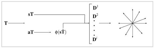
Figure 1: Each tensor T of every order up to dimension three can be decomposed into a set of vectors (of different length or a set of vectors and scalars). First, it must be decomposed into its symmetric part sT and its asymmetric part aT. For the asymmetric part an isomorphism can be used to represent this part also with a symmetric tensor $\textbf{s}\hat{\textbf{T}}$. These symmetric tensors can be decomposed in deviators $\textbf{D}^{j}$. Each of these deviators can be witten as the symmetrization of a set of vectors, called multipoles, multiplied by a scalar.

6 Multipoles

We complete our description by decomposing deviators even further as tensor products of vectors which are called multipoles. This result was first described by Maxwell [5], who found it as an elegant geometric description of spherical harmonics. Using a theorem by Sylvester [13], Maxwell stated in our terms that for any three-dimensional deviator $\mathds{D}$ of order $q$, there are $q$ unit real vectors $\textbf{n}_{1},\dots,\textbf{n}_{q}$ called multipoles and a real non-negative number $a$ such that

$$\mathds{D}=a\,\lfloor\textbf{n}_{1}\otimes\dots\otimes\textbf{n}_{q}\rfloor$$ (23)

The unit vectors $\textbf{n}_{i}$ are uniquely defined by $\mathds{D}$ up to an even number of sign changes, and the number $a$ is unique.

The major algorithmic task is to actually compute the multipoles of all deviators in the deviatoric decomposition of a given tensor. To identify multipoles of a $q$^th-order deviator, Zou et al. [14] define a polynomial of degree $2q$ over the complex numbers by

$$a_{q,0}+\sum\limits_{r=1}^{q}\sqrt{\frac{q!q!}{(q+r)!(q-r)!}}\left(x^{r}\overline{a_{q,r}}+(-1)^{r}x^{-r}a_{q,r}\right)=0.$$ (24)

We do not explain the background of this polynomial here, but refer the reader interested in such detail to the original paper by Zou et al [15]. There, one can see that the polynomial is based on the construction of an orthogonal basis of the corresponding space of deviators for each $x\in\mathds{C}$ and each order $q$. The coefficients $a_{q,r}$, $r=0,\ldots,q$ of the polynomial are the coefficients of the deviator expressed in terms of the basis. The idea is that a root of the polynomial selects a basis that allows one to read off the multipoles. The coefficients $a_{q,r}$ for an explicit example are given in subsubsection 8.1.2. However, the roots of the above polynomial come in pairs as $\overline{x}_{r}^{-1}$ is a root if $x_{r}$ is a root. Therefore, we actually get $2\cdot q$ different roots, but we need only one member of each pair to compute the multipoles. The multipoles of our deviators are found via

$$x_{r}=e^{i\varphi_{r}}\tan\frac{\theta_{r}}{2}$$ (25)

$$\textbf{n}_{r}=\textbf{e}_{3}\cos(\theta_{r})+(\textbf{e}_{1}\cos\varphi_{r}+\textbf{e}_{2}\sin\varphi_{r})\sin\theta_{r}\quad r=1,\dots 8.$$ (26)

7 Second-order tensor decomposition

Based on the general considerations above, we now study the important special case of a second-order tensor to apply the method on familiar ground. A general second-order tensor can be decomposed into the zeroth-order deviator $d$, the first-order deviator d and the second-order deviator D by

$$T_{ij}=dI_{ij}+\varepsilon_{ijk}\cdot d_{k}+D_{ij},\quad d=\frac{1}{3}T_{ii},\quad d_{i}=\frac{1}{2}\varepsilon_{ijk}T_{jk}$$ (27)

$\bm{\varepsilon}$ describes the third-order permutation tensor and I the second-order identity tensor. If $\mathbf{T}$ is symmetric the antisymmetric part represented by d becomes zero.

7.1 Relation to the Eigendecomposition

In the second-order three-dimensional symmetric tensor case, the tensor T can be decomposed by the spectral decomposition into three vectors $\textbf{v}_{i}$ and three scalars $\lambda_{i}$

$$\textbf{T}=\sum\limits_{i=1}^{3}\lambda_{i}\textbf{v}_{i}\otimes\textbf{v}_{i}$$ (28)

or by the deviatoric decomposition into two vectors $\textbf{m}_{1}$ and $\textbf{m}_{2}$ and two scalars $d$ and $a$

$$\textbf{T}=d\cdot\textbf{I}+a\lfloor\textbf{m}_{1}\otimes\textbf{m}_{2}\rfloor$$ (29)

This suggests there is a connection between the two decompositions. This connection is analyzed in the sequel. On the one hand, there are three orthonormal eigenvectors and three real eigenvalues that describe such a tensor. On the other hand, there are two multipoles $\textbf{m}_{1}$ and $\textbf{m}_{2}$ that describe the second-order deviator of this tensor. Together with the isotropic part, i.e. trace times identity, this is the deviatoric decomposition of this tensor. However, because eigendecomposition, deviatoric decomposition and multipole decomposition of deviators are all unique, there must be a connection. This will be elaborated on in this section.

There are three different cases for the position of two multipoles.

Case 1. The scalar $a$ from Eq. (23) equals zero or the multipoles are given by $\textbf{m}_{1}=\textbf{m}_{2}=\left(0,0,0\right)^{\text{T}}$. This is the case, if and only if the tensor has a triple eigenvalue, i.e. is an isotropic or spherical tensor.

Case 2. The multipoles $\textbf{m}_{1}$ and $\textbf{m}_{2}$ are identical, if and only if the tensor has a double eigenvalue. Then, the multipoles are given by the eigenvector according to the eigenvalue with the largest absolute value.

Proof idea. Assume $\textbf{m}_{1}=\textbf{m}_{2}=:\textbf{m}$. Then

$$\textbf{T}=\text{tr}(\textbf{T})\textbf{I}+a\lfloor\textbf{m}\otimes\textbf{m}\rfloor$$ (30)

We know that adding a multiple of the identity to a tensor does not change the eigenvectors of a tensor and does not change the multiplicity of the eigenvalues, so we define $\textbf{m}_{1}\cdot\textbf{m}_{2}=:b$. Because the multipoles are the same, the symmetrization of the tensor product is the tensor product itself and reads

$$a\lfloor\textbf{n}\otimes\textbf{n}\rfloor=\underbrace{a\begin{pmatrix}m_{1}^{2}&m_{1}m_{2}&m_{1}m_{3}\\ m_{1}m_{2}&m_{2}^{2}&m_{2}m_{3}\\ m_{1}m_{3}&m_{2}m_{3}&m_{3}^{2}\end{pmatrix}}_{=:\textbf{M}}-ab\textbf{I}$$ (31)

The eigenvalues of M are given by

$$\lambda_{1}=0,\quad\lambda_{2}=0,\quad\lambda_{3}=a\cdot(m_{1}^{2}+m_{2}^{2}+m_{3}^{2}).$$ (32)

Thus, the tensor has a double eigenvalue.

Assume now, the tensor is degenerated and $s$ is the double eigenvalue. Zheng [16] states that a degenerate second-order three-dimensional tensor can be represented by

$$T=s\textbf{I}\pm\textbf{V}\cdot\textbf{V}^{\text{T}}$$ (33)

where V is defined by the eigenvector to the single eigenvalue by $\textbf{e}=\textbf{V}/\left\lVert\textbf{V}\right\rVert$. It follows

$$\textbf{V}\textbf{V}^{\text{T}}=\textbf{e}\left\lVert\textbf{V}\right\rVert\cdot\left(\textbf{e}\left\lVert\textbf{V}\right\rVert\right)^{\text{T}}=\left\lVert\textbf{V}\right\rVert^{2}(\textbf{e}\cdot\textbf{e}^{\text{T}})=\left\lVert\textbf{V}\right\rVert^{2}\begin{pmatrix}e_{1}^{2}&e_{1}e_{2}&e_{1}e_{3}\\ e_{1}e_{2}&e_{2}^{2}&e_{2}e_{3}\\ e_{1}e_{3}&e_{2}e_{3}&e_{3}e_{3}\end{pmatrix}$$ (34)

We can derive $\textbf{m}_{1}=\textbf{m}_{2}=\textbf{e}$. Therefore, the multipoles collapse into one vector and equal the eigenvector corresponding to the eigenvalue with the largest absolute value, which is in this case the single eigenvalue. Thus, the assumption is true.

Case 3. When the multipoles $\textbf{m}_{1}$ and $\textbf{m}_{2}$ are different, a connection between the eigenvectors and eigenvalues of the symmetric part and the multipoles can be found. The eigenvector deduced by the, according to the absolute value, largest eigenvalue and the, sorted by absolute value, medium eigenvalue are the bisecting lines of the two multipoles. The eigenvector associated to the eigenvalue with largest absolute value is the bisecting line which has the smaller angle to the multipoles. In other words, the closer two of the eigenvalues become, the closer the multipoles bias towards the direction of the largest (absolute) eigenvalue. In the eigenvector system where $\left|\lambda_{1}\right|>\left|\lambda_{2}\right|>\left|\lambda_{3}\right|$, the multipoles are given by

$$\mathbf{m}_{1}=\pm\begin{pmatrix}\sqrt{\frac{2\lambda_{1}+\lambda_{2}}{a}}\\ \sqrt{\frac{-\lambda_{1}-2\lambda_{2}}{a}}\\ 0\end{pmatrix}\qquad\mathbf{m}_{2}=\pm\begin{pmatrix}\sqrt{\frac{2\lambda_{1}+\lambda_{2}}{a}}\\ -\sqrt{\frac{-\lambda_{1}-2\lambda_{2}}{a}}\\ 0\end{pmatrix}$$ (35)

The angle between the first multipole and the eigenvector $\textbf{e}_{1}$ is given by

$$\arccos\left(\frac{\sqrt{\frac{2\lambda_{1}+\lambda_{2}}{a}}}{\sqrt{\frac{\lambda_{1}-\lambda_{2}}{a}}}\right).$$ (36)

Proof idea. Let $\left|\lambda_{1}\right|>\left|\lambda_{2}\right|>\left|\lambda_{3}\right|$, where $\lambda_{i}$ are the eigenvalues of the deviator. Because the deviator is traceless, $\lambda_{3}=-(\lambda_{1}+\lambda_{2})$ holds. The idea for proving the other cases is analogous. Assume, the eigenvectors are given by the coordinate axes $\textbf{e}_{1},\,\textbf{e}_{2},\,\textbf{e}_{3}$. Then the deviator D is given by

$$\textbf{D}=\text{diag}\,(\lambda_{1},\lambda_{2},\lambda_{3})$$

This tensor can also be written as

$$\begin{split}\textbf{D}&=a\begin{pmatrix}\sqrt{\frac{2\lambda_{1}+\lambda_{2}}{a}}^{2}&0&0\\ 0&-\sqrt{\frac{-\lambda_{1}+2\lambda_{2}}{a}}^{2}&0\\ 0&0&0\end{pmatrix}-\frac{a}{3}\left(\frac{2\lambda_{1}+\lambda_{2}}{a}-\frac{-\lambda_{1}-2\lambda_{2}}{a}\right)\textbf{I}\end{split}$$ (37)

Using (35) it follows

$$\textbf{D}=a\cdot\lfloor\textbf{m}_{1}\otimes\textbf{m}_{2}\rfloor$$

Then, the rotation invariance must be proven and the result follows through the equivalence of each step.

This connection underlines the importance of the multipoles. We do not claim that the multipole decomposition is better than the eigendecomposition. We just want to demonstrate that in the symmetric second-order case, the information in the eigendecomposition can also be found in the multipole decomposition. Thus, an analysis of higher-order tensors by using the deviatoric decomposition appears reasonable. With this connection, we want to emphasize the close connection between the two decompositions to show the importance of multipoles, in particular as they allow a generalization to tensors not amenable to an eigendecomposition.

8 Fourth-order tensor decomposition

The deviatoric decomposition described above can be used for every tensor of any order up to dimension three. Backus [6] gave a decomposition of a general fourth-order three-dimensional tensor. It can be decomposed into a fourth-order deviator $\mathcal{D}$, three third-order deviators $\mathrm{D}^{(i)}$, six second-order deviators $D^{(i)}$, six first-order deviators $\mathbf{d}^{(i)}$ and three zeroth-order ones $d^{(i)}$. The tensor is then given by

$$\begin{split}\mathcal{T}_{ijkl}=&D_{ijkl}\\ &+\varepsilon_{ikm}D^{(1)}_{jlm}+\varepsilon_{jkm}D^{(1)}_{ilm}+\varepsilon_{ilm}D^{(1)}_{jkm}+\varepsilon_{jlm}D^{(1)}_{ikm}\\ &+D^{(2)}_{ijm}\varepsilon_{mkl}\\ &+D^{(3)}_{klm}\varepsilon_{mij}\\ &+\delta_{ij}D^{(1)}_{kl}+\delta_{kl}D^{(1)}_{ij}+\delta_{ik}D^{(1)}_{jl}+\delta_{jl}D^{(1)}_{ik}+\delta_{il}D^{(1)}_{jk}+\delta_{jk}D^{(1)}_{il}\\ &+\delta_{ij}D^{(2)}_{kl}+\delta_{kl}D^{(2)}_{ij}-\frac{1}{2}\delta_{ik}D^{(2)}_{jl}-\frac{1}{2}\delta_{jl}D^{(2)}_{ik}-\frac{1}{2}\delta_{il}D^{(2)}_{jk}-\frac{1}{2}\delta_{jk}D^{(2)}_{il}\\ &+\delta_{ij}D^{(3)}_{kl}-\delta_{kl}D^{(3)}_{ij}\\ &+D^{(4)}_{ik}\delta_{jl}+D^{(4)}_{jk}\delta_{il}-D^{(4)}_{il}\delta_{jk}-D^{(4)}_{jl}\delta_{ik}\\ &+D^{(5)}_{ki}\delta_{lj}+D^{(5)}_{li}\delta_{kj}-D^{(5)}_{kj}\delta_{lj}-D^{(5)}_{lj}\delta_{kj}\\ &+D^{(6)}_{ik}\delta_{jl}-D^{(6)}_{il}\delta_{jk}\\ &+(\varepsilon_{ikm}\delta_{jl}+\varepsilon_{jkm}\delta_{il}+\varepsilon_{ilm}\delta_{jk}+\varepsilon_{jlm}\delta_{ik})d^{(1)}_{m}\\ &+d^{(2)}_{i}\varepsilon_{jkl}+d^{(2)}_{j}\varepsilon_{ikl}-\frac{2}{3}\delta_{ij}\varepsilon_{klm}d^{(2)}_{m}\\ &+d^{(3)}_{k}\varepsilon_{lij}+d^{(3)}_{l}\varepsilon_{kij}-\frac{2}{3}\delta_{kl}\varepsilon_{ijm}d^{(3)}_{m}\\ &+\delta_{ij}\varepsilon_{klm}d^{(4)}_{m}\\ &+\delta_{kl}\varepsilon_{ijm}d^{(5)}_{m}\\ &+\varepsilon_{ijk}d^{(6)}_{l}-\varepsilon_{ijl}d^{(6)}_{k}-\varepsilon_{kli}d^{(6)}_{j}+\varepsilon_{klj}d^{(6)}_{i}\\ &+d^{(1)}(\delta_{ij}\delta_{kl}+\delta_{ik}\delta_{jl}+\delta_{il}\delta_{jk})\\ &+d^{(2)}(\delta_{ij}\delta_{kl}-\frac{1}{2}\delta_{ik}\delta_{jl}-\frac{1}{2}\delta_{il}\delta_{jk})\\ &+d^{(3)}(\delta_{ik}\delta_{jl}-\delta_{il}\delta_{jk})\end{split}$$ (38)

This decomposition is very complex, but for tensors with some kinds of symmetries, some of the deviators vanish.

8.1 Stiffness Tensor

The best known application of the deviatoric decomposition is the calculation of symmetries of materials described by the stiffness tensor. To understand the background of this calculation we give a short introduction to the tensor.

We describe the stress at a point of the deformed material by the symmetric second-order Cauchy stress tensor $\bm{\sigma}$ and the strain by $\bm{\varepsilon}$

$$\bm{\sigma}=\begin{pmatrix}\sigma_{11}&\sigma_{12}&\sigma_{13}\\ \sigma_{12}&\sigma_{22}&\sigma_{23}\\ \sigma_{13}&\sigma_{23}&\sigma_{33}\end{pmatrix},\qquad\bm{\varepsilon}=\begin{pmatrix}\varepsilon_{11}&\varepsilon_{12}&\varepsilon_{13}\\ \varepsilon_{12}&\varepsilon_{22}&\varepsilon_{23}\\ \varepsilon_{13}&\varepsilon_{23}&\varepsilon_{33}\end{pmatrix}$$ (39)

The eigenvectors of $\bm{\sigma}$ are called principal stress directions and the eigenvalues principal stresses.

The stiffness tensor describes the linear mapping from strain increments into stress increments which can be described by the Hooke’s law

$$\text{d}\bm{\sigma}=\mathbfcal{C}\mathbf{:}\text{d}\bm{\varepsilon}.$$ (40)

It is a fourth-order three-dimensional tensor and can be represented as $3\times 3\times 3\times 3$ array. Assuming a non-polar material such that the Cauchy stress tensor is symmetric, and the existence of a scalar potential $\psi$ from which stresses are derived by differentiation with respect to a work-conjugate symmetric deformation measure, the stiffness tensor has the two minor symmetries and the major symmetry. Under these conditions, the number of independent coordinates reduces from 81 to 21.

8.1.1 Deviatoric Decomposition

The deviatoric decomposition of the stiffness tensor can for example be used to compute all symmetry planes for all symmetry classes. Hergl et al. [17] used this fact to visualize the symmetries of the stiffness tensor by designing a glyph. Since our stiffness tensor is not totally symmetric, we also need a decomposition of the asymmetric part which was the major achievement of Backus in his paper. Let $\mathcal{C}$ be a three-dimensional fourth-order tensor with major and minor symmetry. Then, the totally symmetric and the asymmetric parts are given by

$$S_{ijkl}=\frac{1}{3}\left(C_{ijkl}+C_{iklj}+C_{iljk}\right),\quad A_{ijkl}=\frac{2}{3}C_{ijkl}-\frac{1}{2}C_{iklj}-\frac{1}{3}C_{iljk}$$ (41)

The trick, to represent the antisymmetric part by deviators, is to define an isomorphism between the second-order totally symmetric tensors $\mathbf{S}^{2}$ and the fourth-order asymmetric tensors $\mathbfcal{A}^{4}$. Let $\mathbf{R}$ be a totally symmetric tensor of order two in three dimensions. We define the isomorphism $\phi$ by

$$\phi(R)_{ijkl}=\delta_{ij}R_{kl}+\delta_{kl}R_{ij}-\frac{1}{2}\delta_{ik}R_{jl}-\frac{1}{2}\delta_{jl}R_{ik}-\frac{1}{2}\delta_{il}R_{jk}-\frac{1}{2}\delta_{jk}R_{il}$$ (42)

This isomorphism is the only possible linear isomorphism that is rotation invariant for any rigid rotation which was proven by Backus using the classification of all isotropic tensors by Weyl [18]. Using (42), the second-order tensor $\mathbf{R}$ is given by

$$R_{ij}=\frac{1}{(n-2)}A_{ijll}-\frac{\delta_{ij}}{2(n-1)(n-2)}A_{kkll}$$ (43)

and the fourth-order three-dimensional tensor $\mathbfcal{C}$ can be represented by the deviatoric decomposition

$$\mathbfcal{C}=\mathbfcal{D}+6\textbf{s}(\textbf{ID})+3\textbf{s}(\textbf{II}d)+\phi(\hat{\textbf{D}})+\frac{1}{2}\phi(\textbf{I}\hat{d})$$ (44)

where $\textbf{R}=\textbf{D}^{2}+\textbf{I}\hat{d}$ is the deviatoric decomposition of the totally symmetric tensor R. Therefore, the stiffness tensor can be uniquely decomposed into one fourth-order deviator $\mathbfcal{D}$, two second-order deviators $\textbf{D}^{1}$ and $\textbf{D}^{2}$ and two zeroth-order deviators $d$ and $\hat{d}$.

Finally, let us shortly denote the complete deviatoric decomposition of the stiffness tensor $\mathbfcal{C}$ in terms of its coefficients which allows to implement it even without understanding the theory in this section. The two zeroth-order deviators are called Lamé coefficients in engineering and can be computed as

$$\lambda=d=\frac{1}{15}\left(2C_{iikk}-C_{ikik}\right),\qquad\mu=\hat{d}=\frac{1}{30}\left(3C_{ikik}-C_{iikk}\right).$$ (45)

The two second-order deviators can be calculated by

$$D_{ij}=\frac{5}{7}\left(C_{kkjj}-\frac{1}{3}C_{kkll}\delta_{ij}\right)-\frac{4}{7}\left(C_{kiki}-\frac{1}{3}C_{klkl}\delta_{ij}\right),$$ (46)

$$\hat{D}_{ij}=\frac{3}{7}\left(C_{kikj}-\frac{1}{3}C_{klkl}\delta_{ij}\right)-\frac{2}{7}\left(C_{kkij}-\frac{1}{3}C_{kkll}\delta_{ij}\right)$$ (47)

This allows to compute the fourth-order deviator by removing the other parts of the deviatoric decomposition

$$\begin{split}D_{ijkl}&=C_{ijkl}-\left(\lambda\delta_{ij}\delta_{kl}+\mu(\delta_{ik}\delta_{jl}+\delta_{il}\delta_{jk})+\delta_{ij}D_{kl}\right.\\ &\left.+\delta_{kl}D_{ij}+\left(\delta_{ik}\hat{D}_{jl}+\delta_{il}\hat{D}_{jk}+\delta_{jk}\hat{D}_{il}+\delta_{jl}\hat{D}_{ik}\right)\right)\end{split}$$ (48)

with the Kronecker delta $\delta_{ij}$.

As a side comment, one can also use this decomposition to calculate Young’s modulus $E(\textbf{d})$ in a specified direction d. Basically, the Young’s modulus describes the stiffness upon uniaxial stretching in this direction. Böhlke and Brüggemann [19] calculated it by

$$\frac{1}{E(\textbf{d})}=\frac{1}{E^{RI}}+6\textbf{D}\cdot\textbf{d}\otimes\textbf{d}+\textbf{d}\otimes\textbf{d}\cdot\mathcal{D}:(\textbf{d}\otimes\textbf{d})$$ (49)

where $E^{RI}=1/(2\mu+\lambda)$ is used to normalize the directional dependent quantities.

8.1.2 Multipole Decomposition

Starting with a stiffness tensor given by its 21 coefficients in arbitrary Cartesian coordinates, the deviatoric decomposition (44) and the multipole representation (23) of the stiffness tensor can be used to calculate the position of the symmetry planes of any anisotropic material.

To calculate the multipoles the equation (24) is used. For the second order deviators $\mathbf{D}=\mathbf{D}^{1}$ and $\hat{\mathbf{D}}=\mathbf{D}^{2}$, we set $q=2$ and

$$\begin{split}&a_{2,0}^{k}=-\sqrt{\frac{3}{2}}(D_{11}^{k}+D_{22}^{k}),\quad a_{2,1}^{k}=D_{13}^{k}-iD_{23}^{k}\\ &a_{2,2}^{k}=\frac{1}{2}(D_{11}^{k}-D_{22}^{k})-iD_{12}^{k}\end{split}$$ (50)

where $k=1,2$. For the fourth-order deviator $\mathcal{D}$, we use $q=4$ and

$$\begin{split}&a_{4,0}=\sqrt{\frac{35}{8}}\left(D_{1111}+D_{2222}+2D_{1122}\right)\\ &a_{4,1}=\sqrt{\frac{7}{2}}(-D_{2213}-D_{1113}+i(D_{2223}+D_{1123}))\\ &a_{4,2}=\frac{\sqrt{7}}{2}(D_{2222}-D_{1111}+2i(D_{2212}+D_{1112}))\\ &a_{4,3}=\frac{1}{\sqrt{2}}(D_{1113}-3D_{2213}-i(3D_{1123}-D_{2223}))\\ &a_{4,4}=\frac{1}{4}D_{1111}+\frac{1}{4}D_{2222}-\frac{3}{2}D_{1122}+i(D_{2212}-D_{1112})\end{split}$$ (51)

We need the complex roots of these three polynomials. In the second-order case, we can use the known formula for quadratic equations to solve for its four roots. In the fourth-order case, we need to use a numerical method to find the eight roots. We use Laguerre’s method to calculate the roots given by Press et al. [20]. The multipoles can be calculated by using (25) and (26).

8.1.3 Anisotropy Type

One of the useful applications of the multipole decomposition is to compute the anisotropy type of the stiffness tensor. For that purpose, the symmetry planes of each deviator must be calculated. The intersection of these are the symmetry planes of the stiffness tensor and determine the anisotropy type.

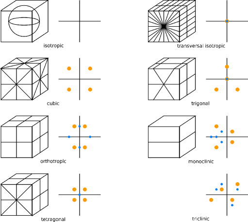
Figure 2: Anisotropy Classes of the stiffness tensor. Left: The symmetry planes of the material in this point. Right: The symmetries of the multipoles (yellow: fourth-order, blue: second-order).

A general stiffness tensor describes a rather complicated relation between stress and strain despite its linear form due to its incremental definition. In practice, most engineering materials exhibit symmetries that simplify this relation further. Of special interest are materials showing symmetry change under load.

In this context, a plane symmetry means that the elastic behavior, i.e. the stress-strain relation does not change under a reflection at this plane. The simplest materials are isotropic. In this case, any plane is a symmetry plane and the relation between strain and stress is the same for all directions. In this case, one needs only the two Lamé coefficients in Eq. (45) to describe the relation. In a linear setting, $\lambda$ enters the scalar relation between a uniform compression and isostatic pressure, and $\mu$ describes the scalar relation between any volume-preserving (i.e. isochoric or deviatoric) strain and isochoric stress with the same direction.

In the general case, engineers distinguish the following different classes of symmetries: isotropic, transversally isotropic, cubic, tetragonal, orthotropic, monoclinic, trigonal and triclinic materials. Of course, these characterizations hold only pointwise if the material exhibits different symmetry types at different positions. In the following, we give a short characterization of all classes. A more comprehensive treatment can be found in textbooks on solid mechanics such as [21].

A second-order deviator can either be isotropic, transversally isotropic or orthogonal. The set of symmetry plane normals $\text{MP}[\textbf{D}^{1}]$ in these three cases is given by

$$\text{MP}[\textbf{D}^{1}]=\begin{cases}\text{all directions}&\text{if }A_{1}=0\\ \{\textbf{n},\textbf{m}_{\varphi},\varphi\in[0,2\pi)\}&\text{if }A_{1}\neq 0,\,\textbf{n}_{1}=\textbf{n}_{2}=\textbf{n}\\ \mathbf{N}_{1},\mathbf{N}_{2},\mathbf{N}_{3}&\text{if }A_{1}\neq 0,\,\textbf{n}_{1}\neq\textbf{n}_{2}\end{cases}$$ (52)

where the infinite set $\{\textbf{m}_{\varphi}\}$ contains all vectors orthogonal to $\mathbf{n}$, and $\textbf{N}_{1},\,\textbf{N}_{2},\,\textbf{N}_{3}$ are given by

$$\textbf{N}_{1}=\frac{\textbf{n}_{1}+\textbf{n}_{2}}{\left|\textbf{n}_{1}+\textbf{n}_{2}\right|},\quad\textbf{N}_{2}=\frac{\textbf{n}_{1}\times\textbf{n}_{2}}{\left|\textbf{n}_{1}\times\textbf{n}_{2}\right|},\quad\textbf{N}_{3}=\textbf{N}_{1}\times\textbf{N}_{2}$$ (53)

The set $\text{MP}[\textbf{D}^{2}]$ can be calculated equivalently using the multipoles $\textbf{n}_{3},\textbf{n}_{4}$.

The set $\text{MP}[\mathcal{D}]$ is a bit more complicated. We follow the description in Zou et al. [14]. If the deviator $\mathcal{D}$ is transversally isotropic the normals are all the same $\textbf{n}_{5}=\textbf{n}_{6}=\textbf{n}_{7}=\textbf{n}_{8}=\textbf{n}$. The symmetry plane normals can be calculated like these in the second-order transversally isotropic deviator case.
If the deviator has cubic symmetry, the cube is given by a right-hand coordinate system $\left\{\textbf{m}_{1},\textbf{m}_{2},\textbf{n}\right\}$ such that the axis direction set $\left\{\textbf{n}_{5},\textbf{n}_{6},\textbf{n}_{7},\textbf{n}_{8}\right\}$ is given by

$$\begin{split}\left\{\frac{\textbf{n}+\textbf{m}_{1}+\textbf{m}_{2}}{\sqrt{3}},\frac{\textbf{n}-\textbf{m}_{1}+\textbf{m}_{2}}{\sqrt{3}},\frac{\textbf{n}+\textbf{m}_{1}-\textbf{m}_{2}}{\sqrt{3}},\frac{-\textbf{n}+\textbf{m}_{1}+\textbf{m}_{2}}{\sqrt{3}}\right\}\end{split}$$ (54)

and the nine symmetry planes are the three coordinate planes and the six planes created by rotating in each of the coordinate planes by an angle of $\pm\pi/4$. If the deviator is tetragonal, the four multipoles are the result of a rotation at $90^{\circ}$ around some axis. The symmetry plane normals of $\mathcal{D}$ are given by the vector orthogonal to all multipoles, the multipoles themselves and the vectors that lie with an angle of $45^{\circ}$ between two of the multipoles. If the deviator is trigonal, one normal is orthogonal to the other three, while the other three are coplanar. The coplanar ones result from a rotation around the fourth multipole at $120^{\circ}$. The three coplanar multipoles are the symmetry plane normals. If the deviator is orthogonal, the multipoles result from a rotation of one of the following sets

$$\begin{cases}S_{W}=&\{\textbf{n}(\theta,\varphi),\textbf{n}(\theta,\pi-\varphi),\textbf{n}(\theta,\pi+\varphi),\textbf{n}(\theta,2\pi-\varphi)\};\\ S_{U}=&\{\textbf{n}(\pi/2,\varphi),\textbf{n}(\pi/2,\pi-\varphi)\}\text{ or }\{\textbf{n}(\theta,0),\textbf{n}(\theta,\pi)\}\\ &\text{ or }\{\textbf{n}(\theta,\pi/2),\textbf{n}(\theta,3\pi/2)\};\\ S_{V}=&\{\text{e}_{1}\}\text{ or }\{\textbf{e}_{2}\}\text{ or }\{\textbf{e}_{3}\}\end{cases}$$ (55)

and the symmetry plane normals equal the coordinate surface normals. If all multipoles lie on a plane or there exists a plane that is their mid-separating surface, the normal to this plane is the symmetry plane normal. A triclinic deviator has four arbitrary multipoles not fulfilling any of the above relations and there is no symmetry plane. Finally, the symmetry plane normals of the stiffness tensor are given by the intersection of the symmetry plane normals of three deviators.

$$\text{MP}[\mathcal{C}]=\text{MP}[\textbf{D}]\cap\text{MP}[\hat{\textbf{D}}]\cap\text{MP}[\mathcal{D}]$$ (56)

9 Conclusion

Every tensor of arbitrary order up to dimension three can be described uniquely by a set of vectors and scalars. This is the main statement of this work. This decomposition is not new, but it is neither well known nor well understood. Thus, this general concept has not found its way into natural or engineering sciences and its physical interpretation remains unclear in many areas. As a step towards obtaining such interpretations, we gave a connection between the multipole decomposition and the spectral decomposition of a symmetric three-dimensional second-order tensor. We are sure, there are other interesting facts about this decomposition and we want to motivate more researchers to analyze this decomposition and use it for different examples to explore its application-specific meanings.

References

- [1] David H Laidlaw and Anna Vilanova. New developments in the visualization and processing of tensor fields. Springer Science & Business Media, 2012.
- [2] Ingrid Hotz and Thomas Schultz. Visualization and processing of higher order descriptors for multi-valued data. Springer, 2015.
- [3] Andrea Kratz, Cornelia Auer, Markus Stommel, and Ingrid Hotz. Visualization and analysis of second-order tensors: Moving beyond the symmetric positive-definite case. In Computer Graphics Forum, volume 32, pages 49–74. Wiley Online Library, 2013.
- [4] Mikhail Itskov. Tensor algebra and tensor analysis for engineers. Springer, 2007.
- [5] James Clerk Maxwell. A treatise on electricity and magnetism, volume 1. Clarendon press, 1881.
- [6] George Backus. A geometrical picture of anisotropic elastic tensors. Reviews of geophysics, 8(3):633–671, 1970.
- [7] W-N Zou and Q-S Zheng. Maxwell’s multipole representation of traceless symmetric tensors and its application to functions of high-order tensors. In Proceedings of the Royal Society of London A: Mathematical, Physical and Engineering Sciences, volume 459, pages 527–538. The Royal Society, 2003.
- [8] W-N Zou, Q-S Zheng, D-X Du, and J Rychlewski. Orthogonal irreducible decompositions of tensors of high orders. Mathematics and Mechanics of Solids, 6(3):249–267, 2001.
- [9] W Thomsen Lord Kelvin. Elements of a mathematical theory of elasticity, part 1: On stresses and strains. Philosophical Transactions of the Royal Society, 166:481–498, 1856.
- [10] Morteza M. Mehrabadi and Stephen C. Cowin. Eigentensors of linear anisotropic elastic materials. The Quarterly Journal of Mechanics and Applied Mathematics, 43(1):15–41, 02 1990.
- [11] Thomas Nagel, Uwe-Jens Görke, Kevin M. Moerman, and Olaf Kolditz. On advantages of the Kelvin mapping in finite element implementations of deformation processes. Environmental Earth Sciences, 75(11):937, jun 2016.
- [12] E.P. Wigner. Group theory. Academic Press, New York, 1959.
- [13] James Joseph Sylvester. Note on spherical harmonics. The London, Edinburgh, and Dublin Philosophical Magazine and Journal of Science, 2(11):291–307, 1876.
- [14] W-N Zou, C-X Tang, and W-H Lee. Identification of symmetry type of linear elastic stiffness tensor in an arbitrarily orientated coordinate system. International Journal of Solids and Structures, 50(14-15):2457–2467, 2013.
- [15] W-N Zou and Q-S Zheng. Maxwell’s multipole representation of traceless symmetric tensors and its application to functions of high-order tensors. Proceedings: Mathematics, Physical and Engineering Sciences, pages 527–538, 2003.
- [16] Xiaoqiang Zheng, Xavier Tricoche, and Alex Pang. Degenerate 3d tensors. In Visualization and Processing of Tensor Fields, pages 241–256. Springer, 2006.
- [17] Chiara Hergl, Thomas Nagel, Olaf Kolditz, and Gerik Scheuermann. Visualization of symmetries in fourth-order stiffness tensors. In 2019 IEEE Visualization Conference (VIS), pages 291–295. IEEE, 2019.
- [18] Hermann Weyl. The classical groups. Princeton University Press, 1946.
- [19] Thomas Böhlke and C Brüggemann. Graphical representation of the generalized hooke’s law. Technische Mechanik, 21(2):145–158, 2001.
- [20] William H Press, Saul A. Teukolsky, William T. Vetterling, and Brian P. Flannery. Numerical recipes in c: The art of scientific computing. 1992.
- [21] Stephen C Cowin and Stephen B Doty. Tissue mechanics. Springer Science & Business Media, 2007.