Message-Passing Algorithms and Homology
From Thermodynamics to Statistical Learning

Introduction

The problem of describing the statistics of a large number $x_{i},x_{j}$,… of interacting random variables emerged in physics with Boltzmann’s efforts to lay principles of thermodynamics on statistical grounds, and high dimensional statistics are now expected to provide with reasonable and tractable models in artificial intelligence and biology. Aimed at modelling the emergence of collective behaviours in large assemblies of constituents, the prism of statistics hence shows deep analogies between atoms in a crystal, and neurons in a network.

A probability distribution $p(x)$ on the joint variable $x=(x_{j})_{j\in\Omega}$ is usually assumed to capture all collective phenomena, although a dimensional curse prohibits the computation of expectation values. Local effects on a small subset $\alpha\subseteq\Omega$ of variables may nonetheless be estimated, as the statistics of the local variable $x_{\alpha}=(x_{i})_{i\in\alpha}$ only involve the marginal distribution $p_{\alpha}(x_{\alpha})$. Spontaneous magnetisation, for instance, is given by the expectation value of a single atomic dipole $x_{i}=\pm 1$, subject to interactions within an arbitrary large crystalline network. Accessing marginals is also a crucial step of statistical learning: usually appearing in the gradient of a loss function, they are necessary to guide the update of model parameters. The design of efficient algorithms for marginal estimation is hence of great practical importance. Message-passing algorithms estimate marginals through a parallelised and asynchronous computing scheme, in which a collection of local units communicate until they eventually reach a consensual state. Understanding their connections with algebraic topology was the first motivation of this thesis.

Gibbs random fields are probabilistic models with a local structure described by a collection $X$ of subsets $\alpha,\beta,\gamma,$… of $\Omega$, over which the global distribution $p(x)$ factorises as a product of local functions. We write $p\in{\cal G}(X)$ when there exists a collection of positive factors $(f_{\alpha})$ such that:

$$p(x)=\frac{1}{Z}\prod_{\alpha\in X}f_{\alpha}(x_{\alpha})$$ (1)

Distributions of this form are more often called graphical models in the computer science literature. The hypergraph $X\subseteq\mathcal{P}(\Omega)$ is then represented by the so-called factor graph, depicted in figure 1, formed by joining variable nodes $(x_{i})$ with their associated factor nodes $(f_{\alpha})$. This factorisation is more conveniently viewed at the level of energies, where the hamiltonian $H$ is defined as a sum of local interaction potentials $(u_{\alpha})$, related to the factors by $u_{\alpha}=-\ln f_{\alpha}$:

$$p=\frac{\operatorname{e}^{-H}}{Z}\quad\mathrm{\quad where\quad}\quad H(x)=\sum_{\alpha\in X}u_{\alpha}(x_{\alpha})$$ (2)

The fundamental Legendre duality between the energy function $H(x)$ and its Gibbs distribution $p(x)$ is related to variational principles on entropy and free energy, of which message-passing algorithms yield approximate solutions.

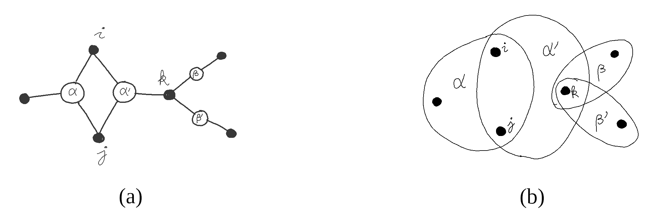
Figure 1: (a) factor graph and (b) hypergraph representations of $X\subseteq\mathcal{P}(\Omega)$.

One of our contributions is to view the Gibbs random field $p\in{\cal G}(X)$ as a homology class of factors. Introducing mutual dependence of variables, overlapping subsets in $X$ also make the parametrisation of $p(x)$ given by equation (1) ambiguous, two collections of factors $(f_{\alpha})$ and $(f^{\prime}_{\alpha})$ defining the same Gibbs random field whenever $\prod_{\alpha}f_{\alpha}\simeq\prod_{\alpha}f^{\prime}_{\alpha}$ up to a scaling factor. This ambiguity is resolved by introducing messages as collections $(m_{\alpha\beta})$ of local functions $m_{\alpha\beta}(x_{\beta})$ for every ordered pair $\alpha\supseteq\beta$ in $X$, and a boundary operator $\partial$ defining factors from messages through:

$$(\partial m)_{\beta}=\prod_{\alpha\supseteq\beta}m_{\alpha\beta}\bigg{/}\prod_{\gamma\subseteq\beta}m_{\beta\gamma}$$ (3)

Assuming $X$ is closed under intersection, we show that $(f_{\alpha})$ and $(f^{\prime}_{\alpha})$ define the same Gibbs random field if and only if there exists $(m_{\alpha\beta})$ such that $f^{\prime}\simeq f\cdot\partial m$ up to scaling. In this view, message-passing algorithms explore a homology class of factors by iterating over messages, the homological constraint expressing conservation of the global distribution $p\in{\cal G}(X)$.

Beliefs $(q_{\alpha})$ are intended to estimate the local marginals $(p_{\alpha})$ of the global probability distribution. These local probabilities should in particular satisfy consistency conditions which require that $q_{\beta}$ is the marginal of $q_{\alpha}$ for every $\beta\subseteq\alpha$. Of cohomological nature, this constraint shall take the form $dq=0$ and is expressed by the following set of equations:

$$q_{\beta}(x_{\beta})=\sum_{y\in E_{\alpha\smallsetminus\beta}}q_{\alpha}(x_{\beta},y)$$ (4)

Defining local probabilities through the local analog of equation (1):

$$q_{\alpha}(x_{\alpha})=\frac{1}{Z_{\alpha}}\prod_{\beta\subseteq\alpha}f^{\prime}_{\beta}(x_{\beta})$$ (5)

the specificity of message-passing algorithms is hence to search for consistent beliefs that derive from homologous factors $f^{\prime}=f\cdot\partial m$. The most general message-passing scheme, belief propagation, assumes the following update rule:

$$m_{\alpha\beta}(x_{\beta})\leftarrow m_{\alpha\beta}(x_{\beta})\cdot\frac{\sum_{y}q_{\alpha}(x_{\beta},y)}{q_{\beta}(x_{\beta})}$$ (6)

Our main contribution is to introduce diffusion equations of the form $\dot{u}=\delta\Phi(u)$ on interaction potentials, which allow to view existing message-passing algorithms as coarse numerical integrators of continuous-time differential equations. The operator $\delta$ is the first-degree boundary of a natural homology theory, acting on a collection of energy fluxes $\varphi_{\alpha\beta}(x_{\beta})$ by:

$$\delta_{\beta}\varphi(x_{\beta})=\sum_{\alpha\supseteq\beta}\varphi_{\alpha\beta}(x_{\beta})-\sum_{\beta\supseteq\gamma}\varphi_{\beta\gamma}(x_{\gamma})$$ (7)

In addition to revealing their deeply homological character, this approach should dramatically improve the stability of message-passing algorithms. Showing belief propagation equivalent to a time-step-one explicit Euler scheme of $\dot{u}=\delta\Phi(u)$, a first and highly advisable improvement is to use a smaller time step $\lambda<1$, which would act as an exponent on the geometric increment of $m_{\alpha\beta}$ in equation (6). As another direction of improvement, we propose a combinatorial correction of messages eliminating their redundancies by extending Möbius inversion formulas to higher degrees. A practical question which shall remain open is whether there exists a notion of optimal transport on $\Phi$ bringing interaction potentials to equilibrium.

Our approach reveals that stationary states of message-passing algorithms lie at the intersection of two constraint surfaces, of homological and cohomological nature respectively. The homological constraint is linear at the level of interaction potentials, and expresses conservation of the total energy:

$$H(x)=\sum_{\alpha\in X}u_{\alpha}(x_{\alpha})$$ (8)

The cohomological constraint $dq=0$, however, is linear at the level of the effective Gibbs states:

$$q_{\alpha}=\frac{\operatorname{e}^{-U_{\alpha}}}{Z_{\alpha}}\mathrm{\quad with\quad}U_{\alpha}(x_{\alpha})=\sum_{\beta\subseteq\alpha}u_{\beta}(x_{\beta})$$ (9)

The problem of describing this intersection is hence highly non-linear, and trying to understand how the geometry of the underlying hypergraph $X$ affects the geometry of message-passing equilibria will lead to difficult questions meeting both algebraic topology and singularity theory.

$$*\quad*\quad*$$

Out of the six chapters contained in this thesis, chapters 1 to 3 review and develop the algebraic theory we shall rely upon. Energy and information functionals are covered in chapter 4, providing background for the central theorem LABEL:cvm characterising solutions of Kikuchi’s cluster variational method [Kikuchi-51] i.e. consistent collections of local probabilities which are critical for a generalised Bethe free energy.

Message-passing algorithms are then addressed in chapter 5, as discrete integrators of continuous-time diffusion equations $\dot{u}=\delta\Phi(u)$. The homological picture allows us to give a rigorous proof of the correspondence theorem LABEL:correspondence between stationary states of belief propagation and solutions of the cluster variational method, as suggested by Yedidia et al. [Yedidia-2005]. Our approach more generally characterises all the flux functionals $\Phi$ for which such a correspondence holds, while the combinatorics developed in chapter 3 lead us to propose another regularisation of the generalised belief propagation algorithm by a degree-one Möbius inversion on the flux functional $\Phi$.

The geometry of message-passing equilibria is finally studied in chapter 6. We describe a class of retractable hypergraphs for which message-passing always converges to the exact marginals of the global probabilistic model to estimate. In general, multiple equilibria may coexist, whose bifurcations are related to singularities of the projection of a smooth manifold of consistent potentials onto their homology classes, and may be tracked in the spectrum of a linearised diffusion operator.

Our first efforts consisted in looking for a formalism in which the elementary operations of message-passing algorithms would fit. The reader is therefore expected to run into some unusual notations and properties, which the following few pages attempt to summarise efficiently. With these in mind, we hope that an informed reader mostly curious of applications might jump directly to chapter 5.

Statistical Systems

A system will be defined by a collection of random variables $x_{i},x_{j},x_{k},\dots$ indexed by labels $i\in\Omega$.

The set of labels $\Omega$ in general has an additional geometric structure describing interactions (e.g. graph or hypergraph).

Subsets $\alpha,\beta,\gamma,\dots$ in $\mathcal{P}(\Omega)$ form a partial order for inclusion, usually denoted in descending alphabetical order:

$$\alpha\supseteq\beta\supseteq\gamma$$

Local Spaces

Given a finite set of microstates $E_{i}$ for every atom/neuron/bit $i\in\Omega$ and a subset of atoms $\alpha\subseteq\Omega$:

• $E_{\alpha}=\prod_{i\in\alpha}E_{i}$ set of local microstates: $x_{\alpha}=(x_{i})_{i\in\alpha}\in E_{\alpha}$

• $A_{\alpha}=\mathbb{R}^{E_{\alpha}}$ algebra of local observables: $f_{\alpha}(x_{\alpha})\in A_{\alpha}$

• $A^{*}_{\alpha}\simeq\mathbb{R}^{E_{\alpha}}$ vector space of local measures: $q_{\alpha}:f_{\alpha}\mapsto\langle\,q_{\alpha}\,|\,f_{\alpha}\,\rangle\in A^{*}_{\alpha}$

• $\Delta_{\alpha}\subseteq A^{*}_{\alpha}$ convex set of positive local probabilities: $p_{\alpha}>0$ and $\sum_{x_{\alpha}}p_{\alpha}(x_{\alpha})=1$

Local Operators

For every $\alpha\subseteq\Omega$ and $\beta\subseteq\alpha$:

• $\pi^{\beta\alpha}:E_{\alpha}\longrightarrow E_{\beta}$ natural projection = restriction $x_{\alpha}\mapsto x_{\beta}$

  $$\pi^{\beta\alpha}:(x_{i})_{i\in\alpha}\mapsto(x_{i})_{i\in\beta}$$

• $j_{\alpha\beta}:A_{\beta}\longrightarrow A_{\alpha}$ natural extension = inclusion $A_{\beta}\subseteq A_{\alpha}$

  $$j_{\alpha\beta}(f_{\beta})(x_{\alpha})=f_{\beta}(x_{\beta})$$

• $\Sigma^{\beta\alpha}:A^{*}_{\alpha}\longrightarrow A^{*}_{\beta}$ partial integration $=$ marginal projection

  $$\Sigma^{\beta\alpha}(q_{\alpha})(x_{\beta})=\sum_{x^{\prime}\in E_{\alpha\smallsetminus\beta}}q_{\alpha}(x_{\beta},x^{\prime})$$

• $\mathbb{E}^{\beta\alpha}_{p_{\alpha}}:A_{\alpha}\longrightarrow A_{\beta}$ conditional expectation w.r.t. $p_{\alpha}\in\Delta_{\alpha}$ given $\beta$

  $$\mathbb{E}^{\beta\alpha}_{p_{\alpha}}(f_{\alpha})(x_{\beta})=\mathbb{E}_{p_{\alpha}}[f_{\alpha}\;|\;x_{\beta}]=\sum_{x^{\prime}\in E_{\alpha\smallsetminus\beta}}\frac{p_{\alpha}(x_{\beta},x^{\prime})\>f_{\alpha}(x_{\beta},x^{\prime})}{p_{\beta}(x_{\beta})}$$

• $\mathbb{F}^{\beta\alpha}:A_{\alpha}\overset{C^{\infty}}{\longrightarrow}A_{\beta}$ conditional free energy of $\alpha$ given $\beta$ = effective energy

  $$\mathbb{F}^{\beta\alpha}(f_{\alpha})(x_{\beta})=-\ln\sum_{x^{\prime}\in E_{\alpha\smallsetminus\beta}}\operatorname{e}^{-f_{\alpha}(x_{\beta},x^{\prime})}$$

Local Duality

• natural duality bracket $\langle\,-\,|\,-\,\rangle:A^{*}_{\alpha}\otimes A_{\alpha}\longrightarrow\mathbb{R}$

  $$\langle\,q_{\alpha}\,|\,f_{\alpha}\,\rangle=\sum_{x_{\alpha}\in E_{\alpha}}q_{\alpha}(x_{\alpha})\,f_{\alpha}(x_{\alpha})$$

• covariance metric $\langle\,-\,|\,-\,\rangle_{p_{\alpha}}:A_{\alpha}\otimes A_{\alpha}\longrightarrow\mathbb{R}$ induced by a local probability $p_{\alpha}\in\Delta_{\alpha}$

  $$\big{\langle}\,f_{\alpha}\,\big{|}\,g_{\alpha}\,\big{\rangle}_{p_{\alpha}}=\mathbb{E}_{p_{\alpha}}\big{[}f_{\alpha}\,g_{\alpha}\big{]}=\sum_{x_{\alpha}\in E_{\alpha}}p_{\alpha}(x_{\alpha})\,f_{\alpha}(x_{\alpha})\,g_{\alpha}(x_{\alpha})$$

Properties

• Adjunction of $\Sigma^{\beta\alpha}$ and $j_{\alpha\beta}$ for the natural duality brackets:

  $$\langle\,\Sigma^{\beta\alpha}(q_{\alpha})\,|\,f_{\beta}\,\rangle=\langle\,q_{\alpha}\,|\,j_{\alpha\beta}(f_{\alpha})\,\rangle$$

• Adjunction of $\mathbb{E}^{\beta\alpha}_{p_{\alpha}}$ and $j_{\alpha\beta}$ for the metric induced by $p_{\alpha}$ on $A_{\alpha}$

  $$\big{\langle}\,\mathbb{E}^{\beta\alpha}(f_{\alpha})\,\big{|}\,g_{\beta}\,\big{\rangle}_{\Sigma^{\beta\alpha}(p_{\alpha})}=\big{\langle}\,f_{\alpha}\,\big{|}\,j_{\alpha\beta}(g_{\beta})\,\big{\rangle}_{p_{\alpha}}$$

• Gibbs state conditional expectations from effective energies: $\mathbb{E}^{\beta\alpha}_{p_{\alpha}}=d\mathbb{F}^{\beta\alpha}_{H_{\alpha}}$

  $$\mathbb{E}_{p_{\alpha}}[f_{\alpha}|x_{\beta}]=\mathbb{F}^{\beta\alpha}(H_{\alpha}+f_{\alpha})-\mathbb{F}^{\beta\alpha}(H_{\alpha})+o(f_{\alpha})\mathrm{\quad for\quad}p_{\alpha}=\frac{1}{Z_{\alpha}}\operatorname{e}^{-H_{\alpha}}$$

Fields

Suppose given a covering $X=\{\alpha,\beta,\gamma,\dots\}$ of $\Omega$ by subsets s.t. $\alpha\cap\beta\in X$ for every $\alpha,\beta\in X$.

$n$-Fields are collections $\{f_{\alpha_{0}\dots\alpha_{n}}\in\mathbb{R}^{E_{\alpha_{n}}}\,|\,\alpha_{0}\supset\dots\supset\alpha_{n}\in X\}$ of local observables indexed by $n$-chains in $X$.

Field Spaces

• $A_{0}(X)=\prod_{\alpha}\mathbb{R}^{E_{\alpha}}$ space of potentials

• $A_{1}(X)=\prod_{\alpha\supset\beta}\mathbb{R}^{E_{\beta}}$ space of currents

• $A_{n}(X)=\prod_{\alpha_{0}\supset\dots\supset\alpha_{n}}\mathbb{R}^{E_{\alpha_{n}}}$ space of local observable $n$-fields

• $\Delta_{0}(X)=\prod_{\alpha}\Delta_{\alpha}\subseteq A^{*}_{0}(X)$ convex space of positive beliefs

• $\Gamma(X)\subseteq\Delta_{0}(X)$ convex subset of consistent beliefs: $p\in\Gamma(X)$ iff $p_{\beta}=\Sigma^{\beta\alpha}(p_{\alpha})$ for all $\alpha\supseteq\beta$.

Differential Operators

• $\delta:A_{1}(X)\longrightarrow A_{0}(X)$ divergence

  $$\delta(\varphi)_{\beta}(x_{\beta})=\sum_{\alpha^{\prime}\supseteq\beta}\varphi_{\alpha^{\prime}\beta}(x_{\beta})-\sum_{\beta\supseteq\gamma^{\prime}}\varphi_{\beta\gamma^{\prime}}(x_{\gamma^{\prime}})$$

• $d:A^{*}_{0}(X)\longrightarrow A^{*}_{1}(X)$ differential

  $$d(q)_{\alpha\beta}(x_{\beta})=q_{\beta}(x_{\beta})-\Sigma^{\beta\alpha}(q_{\alpha})(x_{\beta})$$

• $\nabla_{p}:A_{0}(X)\longrightarrow A_{1}(X)$ gradient w.r.t. to a consistent belief $p\in\Gamma(X)$

  $$\nabla_{p}(f)_{\alpha\beta}(x_{\beta})=f_{\beta}(x_{\beta})-\mathbb{E}^{\beta\alpha}_{p_{\alpha}}(f_{\alpha})(x_{\beta})$$

• $\mathpzc{D}:A_{0}(X)\longrightarrow A_{1}(X)$ effective energy gradient

  $$\mathpzc{D}(f)_{\alpha\beta}(x_{\beta})=f_{\beta}(x_{\beta})-\mathbb{F}^{\beta\alpha}(f_{\alpha})(x_{\beta})$$

Field Duality

• natural duality bracket $\langle\,-\,|\,-\,\rangle:A^{*}_{n}(X)\otimes A_{n}(X)\longrightarrow\mathbb{R}$

  $$\langle\,q\,|\,f\,\rangle=\sum_{\alpha_{0}\supset\dots\supset\alpha_{n}}\langle\,q_{\alpha_{0}\dots\alpha_{n}}\,|\,f_{\alpha_{0}\dots\alpha_{n}}\,\rangle$$

• covariance metric $\langle\,-\,|\,-\,\rangle_{p}:A_{n}(X)\otimes A_{n}(X)\longrightarrow\mathbb{R}$ induced by a consistent $p\in\Gamma(X)$

  $$\big{\langle}\,f\,\big{|}\,g\,\big{\rangle}_{p}=\sum_{\alpha_{0}\supset\dots\supset\alpha_{n}}\big{\langle}\,f_{\alpha_{0}\dots\alpha_{n}}\,\big{|}\,g_{\alpha_{0}\dots\alpha_{n}}\,\big{\rangle}_{p_{\alpha_{n}}}$$

Properties

• Adjunction of $d$ and $\delta$ for the natural duality bracket

  $$\langle\,dq\,|\,\varphi\,\rangle=\langle\,q\,|\,\delta\varphi\,\rangle$$

• Adjunction of $\nabla_{p}$ and $\delta$ for the metric induced by $p\in\Gamma(X)$

  $$\big{\langle}\,\nabla_{p}(f)\,\big{|}\,\varphi\,\big{\rangle}_{p}=\big{\langle}\,f\,\big{|}\,\delta\varphi\,\big{\rangle}_{p}$$

• Gibbs State gradient operator $\nabla_{p}=d\mathpzc{D}_{H}$

  $$\nabla_{p}(f)_{\alpha\beta}=\mathpzc{D}(H+f)_{\alpha\beta}-\mathpzc{D}(H)_{\alpha\beta}+o(f)\mathrm{\quad for\quad}p_{\alpha}=\frac{1}{Z_{\alpha}}\operatorname{e}^{-H_{\alpha}}$$

Combinatorial Operators

• $\tilde{\zeta}_{\Omega}:A_{0}(X)\longrightarrow A_{\Omega}$ total energy

  $$\tilde{\zeta}(h)_{\Omega}(x_{\Omega})=\sum_{\alpha}h_{\alpha}(x_{\alpha})=H_{\Omega}(x_{\Omega})$$

• $\zeta:A_{0}(X)\longrightarrow A_{0}(X)$ zeta transform

  $$\zeta(h)_{\alpha}(x_{\alpha})=\sum_{\alpha\supseteq\beta^{\prime}}h_{\beta^{\prime}}(x_{\beta^{\prime}})=H_{\alpha}(x_{\alpha})$$

• $\mu:A_{0}(X)\longrightarrow A_{0}(X)$ Möbius transform : $\mu=\zeta^{-1}$

  $$\mu(H)_{\alpha}(x_{\alpha})=\sum_{\alpha\supseteq\beta^{\prime}}\mu_{\alpha\beta^{\prime}}\>H_{\beta^{\prime}}(x_{\beta^{\prime}})=h_{\alpha}(x_{\alpha})$$

• $\zeta:A_{n}(X)\longrightarrow A_{n}(X)$ extended zeta transform

  $$\zeta(\varphi)_{\alpha_{0}\dots\alpha_{n}}=\sum_{\alpha_{0}\supseteq\beta_{0}\not\subseteq\alpha_{1}}\dots\sum_{\alpha_{n}\supseteq\beta_{n}}\varphi_{\beta_{0}\dots\beta_{n}}=\Phi_{\alpha_{0}\dots\alpha_{n}}$$

• $\mu:A_{n}(X)\longrightarrow A_{n}(X)$ extended Möbius transform: $\mu=\zeta^{-1}$

  $$\mu(\Phi)_{\alpha_{0}\dots\alpha_{n}}=\sum_{\alpha_{n}\supseteq\beta_{n}}\dots\sum_{\alpha_{0}\supseteq\beta_{0}\not\subseteq\beta_{1}}\mu_{\alpha_{0}\beta_{0}}\dots\mu_{\alpha_{n}\beta_{n}}\>\Phi_{\beta_{0}(\beta_{0}\cap\beta_{1})\dots(\beta_{0}\cap\dots\cap\beta_{n})}=\varphi_{\alpha_{0}\dots\alpha_{n}}$$

Properties

• Möbius numbers $c_{\alpha}\in\mathbb{Z}$ and total energy $H_{\Omega}$ of a potential $h=\mu\cdot H\in A_{0}(X)$

  $$H_{\Omega}=\sum_{\alpha}h_{\alpha}=\sum_{\alpha}c_{\alpha}\>H_{\alpha}=\tilde{\zeta}(h)_{\Omega}$$

• Gauss formula for a current $\varphi\in A_{1}(X)$

  $$\zeta(\delta\varphi)_{\alpha}=\sum_{\alpha\supseteq\beta^{\prime}}\delta(\varphi)_{\beta^{\prime}}=\sum_{\alpha^{\prime}\not\subseteq\alpha}\>\sum_{\alpha\supseteq\beta^{\prime}}\varphi_{\alpha^{\prime}\beta^{\prime}}=\tilde{\zeta}(\varphi)_{\Omega\alpha}$$

• Gauss formula for $\varphi=\mu\cdot\Phi\in A_{1}(X)$

  $$\zeta\big{(}\delta(\mu\cdot\Phi)\big{)}_{\alpha}=\sum_{\alpha^{\prime}\not\subseteq\alpha}c_{\alpha^{\prime}}\>\Phi_{\alpha^{\prime}(\alpha\cap\alpha^{\prime})}=\tilde{\zeta}(\mu\cdot\Phi)_{\Omega\alpha}$$

Main Theorem

• Homology and total energy: for every $u,h\in A_{0}(X)$

  $$\exists\varphi\in A_{1}(X)\mathrm{\quad s.t.\quad}u=h+\delta\varphi\quad\Leftrightarrow\quad\sum_{\alpha}h_{\alpha}=\sum_{\alpha}u_{\alpha}$$

Energy and Information Functionals

Local Functionals

• $\mathbb{F}^{\alpha}:A_{\alpha}\overset{C^{\infty}}{\longrightarrow}\mathbb{R}$ local free energy

  $$\mathbb{F}^{\alpha}(H_{\alpha})=-\ln\sum_{x_{\alpha}\in E_{\alpha}}\operatorname{e}^{-H_{\alpha}(x_{\alpha})}$$

• $S_{\alpha}:\Delta_{\alpha}\overset{C^{\infty}}{\longrightarrow}\mathbb{R}$ local entropy

  $$S_{\alpha}(p_{\alpha})=-\ln\sum_{x_{\alpha}\in E_{\alpha}}p_{\alpha}(x_{\alpha})\>\ln p_{\alpha}(x_{\alpha})$$

Legendre Duality

• $S_{\alpha}$ is the Legendre transform of $\mathbb{F}^{\alpha}$, and reciprocally

  $$\mathbb{F}^{\alpha}(H_{\alpha})=\min_{p_{\alpha}\in\Delta_{\alpha}}\Big{[}\langle\,p_{\alpha}\,|\,H_{\alpha}\,\rangle-S_{\alpha}(p_{\alpha})\Big{]}$$

• $d\mathbb{F}^{\alpha}:A_{\alpha}\overset{C^{\infty}}{\longrightarrow}\Delta_{\alpha}$ maps hamiltonians to their Gibbs probability densities

  $$d\mathbb{F}^{\alpha}(H_{\alpha})=\langle\,p_{\alpha}\,|\,{-}\,\rangle=\mathbb{E}_{p_{\alpha}}[{-}]\mathrm{\quad where\quad}p_{\alpha}=\frac{1}{Z_{\alpha}}\operatorname{e}^{-H_{\alpha}}$$

• $dS_{\alpha}:\Delta_{\alpha}\overset{C^{\infty}}{\longrightarrow}A_{\alpha}/\mathbb{R}$ maps probability densities to their hamiltonians, defined up to additive constants

  $$dS_{\alpha}(p_{\alpha})=\langle\,{-}\,|\,H_{\alpha}\,\rangle\mathrm{\quad where\quad}H_{\alpha}\simeq-\ln p_{\alpha}\mod\mathbb{R}$$

Global Functionals

• ${\cal U}_{\Omega}:\Delta_{\Omega}\times A_{\Omega}\overset{C^{\infty}}{\longrightarrow}\mathbb{R}$ internal energy

  $${\cal U}_{\Omega}(p_{\Omega},H_{\Omega})=\langle\,p_{\Omega}\,|\,H_{\Omega}\,\rangle=\mathbb{E}_{p_{\Omega}}[H_{\Omega}]$$

• $\mathcal{F}_{\Omega}:\Delta_{\Omega}\times A_{\Omega}\overset{C^{\infty}}{\longrightarrow}\mathbb{R}$ variational free energy

  $$\mathcal{F}_{\Omega}(p_{\Omega},H_{\Omega})=\langle\,p_{\Omega}\,|\,H_{\Omega}\,\rangle-S_{\Omega}(p_{\Omega})$$

Bethe-Kikuchi Approximation

• $\check{\mathcal{F}}:\Delta_{0}(X)\times A_{0}(X)\overset{C^{\infty}}{\longrightarrow}\mathbb{R}$ Bethe free energy: constrained to consistent beliefs $p\in\Gamma(X)$

  $$\check{\mathcal{F}}(p,H)=\sum_{\alpha\in X}c_{\alpha}\Big{[}\langle\,p_{\alpha}\,|\,H_{\alpha}\,\rangle-S_{\alpha}(p_{\alpha})\Big{]}$$

Main Theorems

• Homological invariance of $\check{\mathcal{F}}(p,\,-\,)$: for every consistent belief $p\in\Gamma(X)$ and effective hamiltonian $H\in A_{0}(X)$

  $$\check{\mathcal{F}}\big{(}p,H+\zeta(\delta\varphi)\big{)}=\check{\mathcal{F}}(p,H)$$

• $p\in\Gamma(X)$ is critical for $\check{\mathcal{F}}({-},H)_{|\Gamma(X)}$ iff there exists a current $\varphi\in A_{1}(X)$ s.t. for all $\alpha\in X$

  $$-\ln p_{\alpha}\simeq H_{\alpha}+\zeta(\delta\varphi)_{\alpha}\mod\mathbb{R}$$

Message-Passing as Diffusion

Heat Analogy

Energy density = time-dependent scalar field $u:\mathbb{R}\rightarrow\Omega^{0}(\mathbb{R}^{3})=C^{\infty}(\mathbb{R}^{3})$

Heat exchange = time-dependent vector field $\vec{\varphi}:\mathbb{R}\rightarrow\Omega^{1}(\mathbb{R}^{3})=C^{\infty}(\mathbb{R}^{3},\mathbb{R}^{3})$

• energy conservation: $\dot{u}={\rm div}(\vec{\varphi})$

• heat flux: $\vec{\varphi}=-\lambda\>\vec{\rm grad}(T)$

Characteristic relation $u=c\>T$ (condensed matter) or non-relationship between temperature and energy.

Message-Passing on Graphs

The algorithm takes the form $\dot{u}=-\big{(}\delta\circ\mathpzc{D}\circ\zeta\big{)}(u)$ on potentials, i.e.

$$\begin{array}[]{ll|l}\dot{u}=\delta\varphi&\quad\mathrm{\quad where\quad}&\varphi=-\mathpzc{D}(U)\\[3.33328pt] &&U=\zeta\cdot u\end{array}$$

• Energy conservation $\dot{u}=\delta\varphi$ dictates the update of effective potentials $u\in A_{0}(X)$

  $$\frac{d}{dt}u_{ij}(x_{i},x_{j})=-\varphi_{ij\to j}(x_{j})-\varphi_{ij\to i}(x_{i})\mathrm{\quad and\quad}\frac{d}{dt}u_{i}(x_{i})=\sum_{j^{\prime}\sim i}\varphi_{ij^{\prime}\to i}(x_{i})$$

• Heat flux $\varphi=-\mathpzc{D}(U)\in A_{1}(X)$ measures the lack of consistency of effective hamiltonians

  $$\varphi_{ij\to j}(x_{j})=-U_{j}(x_{j})-\ln\sum_{x_{i}\in E_{i}}\operatorname{e}^{-U_{i}(x_{i},x_{j})}$$

• Effective hamiltonians $U=\zeta(u)\in A_{0}(X)$ are given by

  $$U_{ij}(x_{i},x_{j})=u_{ij}(x_{i},x_{j})+u_{i}(x_{i})+u_{j}(x_{j})\mathrm{\quad and\quad}U_{i}(x_{i})=u_{i}(x_{i})$$

• Beliefs $q_{ij}=\frac{1}{Z_{ij}}\operatorname{e}^{-U_{ij}}$ and $q_{i}=\frac{1}{Z_{i}}\operatorname{e}^{-U_{i}}$ should be normalised at each iteration on graphs with loops

Message-Passing on Hypergraphs

Möbius inversion on the heat flux reads $\dot{u}=-\big{(}\delta\circ\mu\circ\mathpzc{D}\circ\zeta\big{)}(u)$ on potentials, i.e.

$$\begin{array}[]{ll|l}\dot{u}=\delta\varphi&\quad\mathrm{\quad where\quad}&\varphi=\mu\cdot\Phi\\[3.33328pt] &&\Phi=-\mathpzc{D}(U)\\[3.33328pt] &&U=\zeta\cdot u\end{array}$$

• Effective hamiltonians $U=\zeta\cdot u\in A_{0}(X)$ follow the energy conservation principle: $\dot{U}=\delta^{\zeta}(\Phi)$ where $\delta^{\zeta}=\zeta\,\delta\,\zeta^{-1}$

  $$\frac{d}{dt}U_{\alpha}(x_{\alpha})=\sum_{\alpha^{\prime}\not\subseteq\alpha}c_{\alpha^{\prime}}\>\Phi_{\alpha^{\prime}(\alpha\cap\alpha^{\prime})}(x_{\alpha\cap\alpha^{\prime}})$$

• Extensive heat flux $\Phi=\zeta\cdot\varphi\in A_{1}(X)$ flows against the effective energy gradient: $\Phi=-\mathpzc{D}(U)$

  $$\Phi_{\alpha\beta}(x_{\beta})=-U_{\beta}(x_{\beta})-\ln\sum_{x^{\prime}\in E_{\alpha\smallsetminus\beta}}\operatorname{e}^{-U_{\alpha}(x_{\beta},x^{\prime})}$$

• Beliefs $q_{\alpha}=\frac{1}{Z_{\alpha}}$ do not need to be normalised

Correspondence Theorem

Effective hamiltonians $U=H+\zeta\cdot\delta\varphi\in A_{0}(X)$ are stationary under diffusion
$\Leftrightarrow\>\>$ Beliefs $q=\frac{1}{Z}\operatorname{e}^{-U}\in\Gamma(X)$ are consistent and critical for the Bethe free energy $\check{\mathcal{F}}({-},H)_{|\Gamma(X)}$

Crystals, Codes and Networks

The following 3 pages give a brief overview of some applications that motivated this thesis. They involve a rather wide spectrum of communities, including statistical physics, artificial intelligence and information theory. Although an extensive coverage of applications is far out of our scope, the book Information, Physics and Computation by Mézard and Montanari [Mezard-Montanari] is an excellent reference for all three subjects.

Crystals and Spin Glasses

Figure 2: (a) Ising model on the square lattice $\mathbb{Z}^{n}$ (b) Spin glasses as in the Sherrington-Kirkpatrick model have random magnetic couplings and release the $\mathbb{Z}^{n}$ symmetry assumption.

A set of atoms $\Omega$ carries a magnetic dipole $x_{i}\in\{\pm 1\}$ for all $i\in\Omega$.

A set of pairs in $\Omega\times\Omega$ relates neighbours $i\sim j$ whose interactions contribute to the total energy of the system.

• Local magnetic field = bias $b_{i}\in\mathbb{R}$

  $$h_{i}(x_{i})=-b_{i}\>x_{i}$$

• Local magnetic coupling = weight $w_{ij}\in\mathbb{R}$

  $$h_{ij}(x_{i},x_{j})=-w_{ij}\>x_{i}x_{j}$$

• Total hamiltonian $H:\{\pm 1\}^{\Omega}\longrightarrow\mathbb{R}$

  $$H(x)=\sum_{i\in\Omega}h_{i}(x_{i})+\sum_{i\sim j}h_{ij}(x_{i},x_{j})$$

• Gibbs state $p^{\theta}:\{\pm 1\}^{\Omega}\longrightarrow\mathbb{R}$ describes statistical equilibrium at inverse temperature $\theta=\frac{1}{k_{B}T}$

  $$p^{\theta}(x)=\frac{\operatorname{e}^{-\theta H(x)}}{\sum_{x^{\prime}}\operatorname{e}^{-\theta H(x^{\prime})}}$$

High temperature limit: if $\theta\to 0$ then $p^{\theta}$ tends to the uniform measure on $\{\pm 1\}^{\Omega}$.

Low temperature limit: if $\theta\to+\infty$ then $p^{\theta}$ tends to a barycenter of Dirac measures on the minima of $H$.

Boltzmann Machines and Neural Networks

Figure 3: Fully-connected (a), restricted (b) and deep (c) Boltzmann machines.

A restricted Boltzmann machine (RBM) consists of two neuron layers $x_{1},\dots,x_{N}\in\{\pm 1\}$ and $y_{1},\dots,y_{P}\in\{\pm 1\}$.

The network is trained to generate configurations on its visible layer $x$, interacting with the hidden layer $y$.

Biases $a_{i},b_{j}\in\mathbb{R}$ and couplings $w_{ij}\in\mathbb{R}$ are learned from observed samples $\bar{x}^{1},\dots,\bar{x}^{n}\in\{\pm 1\}^{N}$ on the visible layer.

• Probability of a configuration $(x,y)\in\{\pm 1\}^{N+P}$ modeled by

  $$p(x,y)=\frac{1}{Z}\operatorname{e}^{-H(x,y)}\mathrm{\quad with\quad}H(x,y)=-\sum_{i=1}^{N}a_{i}x_{i}-\sum_{j=1}^{P}b_{j}y_{j}-\sum_{i=1}^{N}\sum_{j=1}^{P}w_{ij}\;x_{i}y_{j}$$

• Maximise the expected log-likelihood of a training sample $\bar{x}^{1},\dots,\bar{x}^{n}$

  $$\begin{array}[]{lllll}\mathbb{E}_{\bar{x}}[-\ln p(\bar{x})]&=&\displaystyle-\frac{1}{n}\sum_{s=1}^{n}\ln\sum_{y\in\{\pm 1\}^{P}}\operatorname{e}^{-H(\bar{x}^{s},y)}&+&\displaystyle\ln\sum_{x\in\{\pm 1\}^{N}}\sum_{y\in\{\pm 1\}^{P}}\operatorname{e}^{-H(x,y)}\end{array}$$

• Estimate the loss-function gradient along a local variation $h(x,y)=h(x_{i},y_{j})$ of the total energy $H(x,y)$

  $$\begin{array}[]{lllll}\displaystyle\frac{\partial\mathbb{E}_{\bar{x}}[-\ln p(\bar{x})]}{\partial h}&=&\mathbb{E}_{\bar{x}}\big{[}\,\mathbb{E}_{p}\big{[}\,h(\bar{x}_{i},y_{j})\,\big{|}\,\bar{x}\,\big{]}\big{]}&-&\mathbb{E}_{p}\big{[}\,h(x_{i},y_{j})\,\big{]}\\ &=&\displaystyle\frac{1}{n}\sum_{s=1}^{n}\sum_{y_{j}\in\{\pm 1\}}p(y_{j}|\bar{x}^{s})\>h(\bar{x}_{i},y_{j})&+&\displaystyle\sum_{x\in\{\pm 1\}}\sum_{y\in\{\pm 1\}}p(x_{i},y_{j})\>h(x_{i},y_{j})\end{array}$$

Markov properties: conditional independence of $x_{1},\dots,x_{n}$ given $y$ and reciprocally

$$p(x|y)=\prod_{i=1}^{N}p(x_{i}|y)=\prod_{i=1}^{N}\sigma\Big{(}a_{i}x_{i}-\sum_{j}w_{ij}x_{i}y_{j}\Big{)}$$

Gibbs sampling: start from a random configuration $y^{(0)}\in\{\pm 1\}$ … draw $x^{(t+1)}\in\{\pm 1\}^{N}$ from $p(x\,|\,y^{(t)})$ … draw $y^{(t+1)}\in\{\pm 1\}^{P}$ from $p(y\,|\,x^{(t+1)})$ average over time $t$ to get an estimate of $p(x,y)$ and its marginals

Low Density Parity-Check Codes

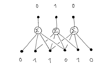
Figure 4: Parity-check codes consist of two sequences $(x_{i})\in\{0,1\}^{N}$ of signal bits (bottom) and $(y_{j})\in\{0,1\}^{P}$ of validation bits (top) computing the sum mod $2$ of a subset of signal bits.

A compressed message is encoded as a binary sequence $(x_{i})\in\{0,1\}^{N}$ followed by a parity-check sequence $(y_{j})\in\{0,1\}^{P}$.

Decoding consists in restoring parity-check consistency to rectify the errors induced by a noisy transmission channel.

• Beliefs $q_{i}(x_{i})$ and $q_{j}(y_{j})$ initially depend on the received values $\bar{x}_{i}$ and $\bar{y}_{j}$ e.g.

  $$q_{i}(x_{i})=\frac{1}{Z_{i}}\operatorname{e}^{-h_{i}(x_{i})}\mathrm{\quad with\quad}h_{i}(x_{i})=\theta\cdot{|x_{i}-\bar{x}_{i}|}$$

• Local potentials $h_{\alpha_{j}}$ for every validation bit $j\in\{1,\dots,P\}$ connected to a subset $\alpha_{j}\subseteq\{1,\dots,N\}$ of signal bits

  $$h_{\alpha_{j}}(x_{i_{1}},\dots,x_{i_{n}},y_{j})=\lambda\cdot\bigg{[}\Big{(}y_{j}-\sum_{i\in\alpha_{j}}x_{i}\Big{)}\>\%\>2\bigg{]}$$

• Local beliefs $q_{\alpha_{j}}$ favorise parity-check consistency and agreement with received values

  $$q_{\alpha_{j}}(x_{i_{1}},\dots,x_{i_{n}},y_{j})=\frac{1}{Z_{\alpha_{j}}}\operatorname{e}^{-H_{\alpha_{j}}(x_{i_{1}},\dots,x_{i_{n}},y_{j})}\mathrm{\quad with\quad}H_{\alpha_{j}}=h_{\alpha_{j}}+h_{j}+\sum_{i\in\alpha_{j}}h_{i}$$

Message-Passing: initialise beliefs according to signal received … compute a message $m_{\alpha_{j}\to j}$ for all $\alpha_{j}$ and messages $m_{\alpha_{j}\to i_{p}}$ for all $i_{p}\in\alpha_{j}$ $$\begin{array}[]{lll}m_{\alpha_{j}\to j}(y_{j})&=\displaystyle\frac{1}{q_{j}(y_{j})}&\displaystyle\sum_{x^{\prime}\in\{0,1\}^{\alpha_{j}}}q_{\alpha_{j}}(x^{\prime}_{i_{1}},\dots,x^{\prime}_{i_{n}},y_{j})\\ m_{\alpha_{j}\to i_{p}}(x_{i_{p}})&=\displaystyle\frac{1}{q_{i_{p}}(x_{i_{p}})}&\displaystyle\sum_{x^{\prime}\in\{0,1\}^{\alpha_{j}\smallsetminus i_{p}}}\>\sum_{y^{\prime}_{j}\in\{0,1\}}q_{\alpha_{j}}(x^{\prime}_{i_{1}},\dots,x_{i_{p}},\dots,x^{\prime}_{i_{n}},y_{j})\end{array}$$ … update beliefs according to incoming messages and normalise $$\begin{array}[]{ll}q_{j}(y_{j})&\leftarrow\;q_{j}(y_{j})\>m_{\alpha_{j}\to j}(y_{j})\\[4.16667pt] q_{i}(x_{i})&\leftarrow\;\displaystyle q_{i}(x_{i})\prod_{\alpha_{j}\ni i}m_{\alpha_{j}\to i}(x_{i})\\ q_{\alpha_{j}}(x_{i_{1}},\dots,x_{i_{n}},y_{p})&\leftarrow\;\displaystyle q_{\alpha_{j}}(x_{i_{1}},\dots,x_{i_{n}})\prod_{i_{p}\in\alpha_{j}}\prod_{\alpha_{k}\ni i_{p}}m_{\alpha_{k}\to i_{p}}(x_{i_{p}})\end{array}$$ loop until computed messages are close to 1 $\Leftrightarrow$ belief consistency is reached

Index of Notations

Functors:

• $X\subseteq\mathcal{P}(\Omega)$ base hypergraph

• $(E,\pi)$ microstates, §2.1.1

• $(A,j)$ observables, §2.2.2

• $(A^{*},\Sigma)$ measures, §2.2.3

• $(\Delta,\Sigma)$ probability densities, §2.2.4

Spaces:

• $A_{\bullet}(X)$ complex of local observables, def. 2.6

• $A^{*}_{\bullet}(X)$ complex of local measures, –

• $\Delta_{\bullet}(X)$ convex subspace of local probabilities, –

• $\Gamma(X)$ convex subspace of consistent local probabilities, def. 2.7

• $\mathcal{C}(X)$ manifold of consistent local hamiltonians, def. LABEL:CU

• ${\cal Z}(X)$ manifold consistent local potentials, def. LABEL:Z

Differential Operators:

• $\delta$ boundary of $A_{\bullet}(X)$, §2.2.2

• $d$ differential of $A^{*}_{\bullet}(X)$, –

• $\mathpzc{D}$ effective energy gradient, §5.2.1

• $\nabla=\mathpzc{D}_{*}$ linearised effective energy gradient –

Combinatorial Operators:

• $\zeta$ zeta transform, sections 3.2 and 3.3

• $\mu=\zeta^{-1}$ Möbius transform, §3.2.1 and 3.3.3

Diffusion Operators:

• $\Phi=-\mathpzc{D}\circ\zeta$ standard diffusion flux, §5.2.2

• $\mathcal{T}=\delta\Phi$ standard diffusion vector field, –

• $\phi=-\mu\circ\mathpzc{D}\circ\zeta$ canonical diffusion flux, §5.3.2

• $\tau=\delta\phi$ canonical diffusion vector field, –

Fields:

• $h,u\in A_{0}(X)$ interaction potentials, $h$ for reference and $u$ for evolution

• $H,U\in A_{0}(X)$ local hamiltonians, $H=\zeta\cdot h$ and $U=\zeta\cdot u$

• $\varphi\in A_{1}(X)$ energy flux

• $q\in\Delta_{0}(X)$ local beliefs, $q_{\alpha}=[\operatorname{e}^{-U_{\alpha}}]$

• $p\in\Gamma(X)$ Gibbs state marginals $p_{\alpha}=\Sigma^{\alpha\Omega}\big{(}p_{\Omega}\big{)}$

Information Functionals:

• $\mathbb{F}^{\alpha}$ free energy, §4.1.1

• $\mathbb{F}^{\beta\alpha}$ effective energy, §4.1.2

• $S$ Shannon entropy, §4.2.1

• $\mathcal{F}$ variational free energy, §4.3.2

• $\check{\mathcal{F}}$ Bethe free energy, §4.3.3

Chapter 1 Homological Algebra

This chapter consists of a short yet self-contained introduction to some of the most remarkable concepts of ${\rm XX^{th}}$ mathematics, which happened to take a definite form simultaneously and for the needs of one another: homology and categories. It still seems quite rare that they belong to a common language with the physicist or the computer scientist, and we hope this chapter provides with more than the necessary material. For the more informed reader, this chapter’s purpose is to relate our construction to the general theory of simplicial groups.

Categories may be thought of as collections of points and arrows, which describe mathematical objects and their relations, while functors consistently transform categories into other categories. Section 1 reviews these elementary definitions and focuses on providing concrete examples such as the categories of groups, vector spaces, topological spaces, programmable types, etc.

The practical use of category theory language is specially remarkable in the characterisation of particular objects by universal properties. Section 2 focuses on the categorical concept of limit, which unifies many constructions such as union and product of sets, sums of vector spaces, inductive and projective limits, etc. It should familiarise the reader with commutative diagrams and will help describe homology groups in chapter 2.

Homology provides a general procedure to extract algebraic invariants from topological spaces, while cohomology may be thought of as an abstraction of differential calculus. Section 3 provides with the basic definition of homology groups, which from a purely algebraic point of view, occur in the study of a square-null operator $d$ such that $d^{2}=0$. Geometry however best illustrates the purpose of homology, which unifies various integration by parts formulas under the Stokes theorem. The Gauss formula is a particular case of the latter, and its discrete analog 2.3 encountered in chapter 2 will play a fundamental role in understanding the geometric structure of message-passing algorithms.

1.1   
Categories and Functors

1.1.1   
Categories

Categories provide with a convenient abstraction of most mathematical constructions and theories. They were introduced by Eilenberg and MacLane [Eilenberg-MacLane] to build homological algebra on a rigorous and flexible ground, they have since proven useful in many diverse applications in mathematics, informatics and physics.

Definition 1.1.

A category ${\bf C}$ is a class of objects $A,B,C,\dots$ denoted by ${\rm Ob}({\bf C})$ together with:

• a set of arrows $\operatorname{Hom}(A,B)$ for every $A,B$ in ${\rm Ob}({\bf C})$,

• an identity arrow $1_{A}\in\operatorname{Hom}(A,A)$ for every $A$ in ${\rm Ob}({\bf C})$,

• a composite arrow $gf\in\operatorname{Hom}(A,C)$ for every $f\in\operatorname{Hom}(A,B)$ and $g\in\operatorname{Hom}(B,C)$

satisfying the following axioms:

1. Identity: for every $f:A\rightarrow B$

   $$f=f\cdot 1_{A}=1_{B}\cdot f$$ (1.1)

2. Associativity: for every $f:A\rightarrow B$, $g:B\rightarrow C$ and $h:C\rightarrow D$

   $$h(gf)=(hg)f$$ (1.2)

The first example of a category is $\mathbf{Set}$, the category whose objects are sets and arrows are functions. When each object of ${\bf C}$ may be viewed as a set and each arrow $f\in\operatorname{Hom}(A,B)$ induces a function $f\in B^{A}$ of the underlying sets, the category ${\bf C}$ is called concrete, Equivalently, a concrete category ${\bf C}$ is a subcategory of $\mathbf{Set}$. Although the following definitions make sense in any category, they respectively correspond to bijections, injections, and surjections in $\mathbf{Set}$ as in most examples of concrete categories.

Definition 1.2.

Let ${\bf C}$ be a category and $f:A\rightarrow B$ a morphism.

• f is an isomorphism if there exists $g:B\rightarrow A$ such that $gf=1_{A}$ and $fg=1_{B}$.

• f is a monomorphism if for all $X$ and $u,u^{\prime}:X\rightarrow A$, $fu=fu^{\prime}$ implies $u=u^{\prime}$.

• f is an epimorphism if for all $Y$ and $v,v^{\prime}:B\rightarrow Y$, $vf=v^{\prime}f$ implies $v=v^{\prime}$.

A category may have terminal objects, satisfying one of the conditions of the following definition. These very special objects are also called universal as a terminal object of a given kind, when it exists, is always defined up to isomorphism. Universal objects are related to the existence of certain limits, and describe many fundamental constructions in algebra and geometry.

Definition 1.3.

Let ${\bf C}$ be a category.

• an object $I$ is initial in ${\bf C}$ if there is a unique arrow $I\rightarrow A$ for every object $A$ in ${\bf C}$,

• an object $F$ is final in ${\bf C}$ if there is a unique arrow $A\rightarrow F$ for every object $A$ in ${\bf C}$,

• an object $O$ is null in ${\bf C}$ if it is both final and initial.

Proposition 1.4.

If $T$ and $T^{\prime}$ are terminal objects of the same kind, then $T$ is isomorphic to $T^{\prime}$.

Proof.

When $T$ is a terminal object, the axioms imply that $1_{T}$ is the unique arrow of $\operatorname{Hom}(T,T)$. If $T^{\prime}$ is terminal of the same kind, the arrows $T\rightarrow T^{\prime}$ and $T^{\prime}\rightarrow T$ must then compose as $1_{T}$ and $1_{T^{\prime}}$. ∎

Definition 1.5.

For any category ${\bf C}$, its dual or opposite category ${\bf C}^{op}$ has the same objects as ${\bf C}$ and, for every arrow $f:A\rightarrow B$ in ${\bf C}$, a reversed arrow $f^{op}:B\rightarrow A$ in ${\bf C}^{op}$.

In the following fundamental examples, we give an initial and a terminal object when they exist. In many interesting examples, the set of morphisms between two objects is also an object of the category. This is not true in general and we precise when it is the case.

Examples of Categories:

1. A partial order $(X,\geq)$ is a category with a unique arrow $x\rightarrow y$ whenever $x\geq y$.

   The identity axiom $x\geq x$ expresses the reflexivity of the order relation, while the transitivity asking that if $x\geq y$ and $y\geq z$, then $x\geq z$, is given by the existence of compositions.

   Initial and final elements correspond to maximal and minimal elements respectively.

2. The category $\mathbf{Set}$ whose objects are sets and arrows are functions.

   The set of arrows $\operatorname{Hom}(A,B)$ is itself a set, denoted $B^{A}$.

   The empty set $\varnothing$ is initial and the point $\bullet=\{\varnothing\}$ is final in $\mathbf{Set}$.

3. The category $\mathbf{Alg}_{\mathbb{K}}$ of unital algebras over a field $\mathbb{K}$ whose arrows are algebra morphisms.

   The field $\mathbb{K}$ is both initial and final in $\mathbf{Alg}_{\mathbb{K}}$, it is a null object.

4. The category $\mathbf{Top}$ whose objects are topological spaces and arrows are continuous functions.

   The point $\bullet$ is final in $\mathbf{Top}$.

5. The category ${\bf Types}$ whose objects are variable types and arrows are programs.

   The set of arrows $\operatorname{Hom}({\tt a},{\tt b})$ represents the programs with input of type ${\tt a}$ and output of type ${\tt b}$. It is itself a type, denoted by $({\tt a\rightarrow b})$.

   The empty or bottom type $\perp$ is initial, while the unit or top type $\top$ is final. An arrow of type ${\tt a}\rightarrow\perp$ represents a program which does not terminate.

6. For every object $X$ of a category ${\bf C}$, the category ${\bf C}_{X}$ above $X$ has arrows $f:A\rightarrow X$ as objects. A morphism $\varphi:f\rightarrow g$ in ${\bf C}_{X}$ between $f:A\rightarrow X$ and $g:B\rightarrow X$ is an arrow $\varphi:A\rightarrow B$ in ${\bf C}$ such that the following diagram commutes:

   (1.3)

   There is a similar category ${\bf C}^{X}$ below $X$ defined by reversing arrows, which amounts to reading the above definition in ${\bf C}^{op}$.

1.1.2   
Functors

Just as morphisms describe relations between objects in a category, functors describe relations between categories by bringing every object to an object and every arrow to an arrow.

Definition 1.6.

A covariant functor $T$ from two categories ${\bf C}$ and ${\bf C}^{\prime}$ is defined by:

• An object $T(A)$ of ${\bf C}^{\prime}$ for every object $A$ of ${\bf C}$

• An arrow $T(f):T(A)\rightarrow T(B)$ in ${\bf C}^{\prime}$ for every arrow $f:A\rightarrow B$ in ${\bf C}$.

satisfying the following axioms:

1. $T(1_{A})=1_{T(A)}$,

2. $T(fg)=T(f)\cdot T(g)$

Examples of Functors:

1. When $(X,\geq)$ and $(Y,\geq)$ are partially ordered sets, a functor from $X$ to $Y$ is an order-preserving map from $X$ to $Y$.

   This defines the category $\mathbf{Ord}$ of ordered sets with order-preserving map as morphisms.

2. For every object $X$ of a category ${\bf C}$, there are canonical functors $\operatorname{Hom}(-,X)$ and $\operatorname{Hom}(X,-)$ from ${\bf C}$ to $\mathbf{Set}$.

   The pull-back of $f:A\rightarrow B$ is the map $f^{*}:\operatorname{Hom}(B,X)\rightarrow\operatorname{Hom}(A,X)$ defined by $f^{*}(u)=u\circ f$ for every $u:B\rightarrow X$. $\operatorname{Hom}(-,X)$ is a contravariant functor.

   The push-out of $g:C\rightarrow D$ is the map $g_{*}:\operatorname{Hom}(X,C)\rightarrow\operatorname{Hom}(X,D)$ defined by $g_{*}(v)=g\circ v$ for every $u:X\rightarrow C$. $\operatorname{Hom}(X,-)$ is a covariant functor.

3. A contravariant functor from $\mathbf{Top}$ to $\mathbf{Alg}$ is defined by associating to each topological space $\Omega$ the algebra $C(\Omega)$ of real continuous functions on $\Omega$.

   For every arrow $\varphi:\Omega\rightarrow\Omega^{\prime}$ in $\mathbf{Top}$, its pullback $\varphi^{*}:C(\Omega^{\prime})\rightarrow C(\Omega)$ defined by $\varphi^{*}(f)=f\circ\varphi$ is an algebra morphism.

   This is a particular case of the previous example, as $C(\Omega)=\operatorname{Hom}(\Omega,\mathbb{R})$ in $\mathbf{Top}$.

4. The endofunctor ${\tt list}$ of ${\bf Types}$ associates to each type ${\tt a}$ the type ${\tt[a]}$ of lists whose elements are of type ${\tt a}$.

   Any function ${\tt f:a\rightarrow b}$ induces a function ${\tt map(f):[a]\rightarrow[b]}$ returning the list of images under ${\tt f}$ of the input list’s elements.

   $$\begin{split}\tt map(f)&:\tt[x,\;\dots xs]\mapsto[f(x),\;\dots map(f)(xs)]\\ &:\tt[\;]\mapsto[\;]\end{split}$$ (1.4)

5. When ${\bf C}$ is a concrete category, there is a canonical forgetful functor from ${\bf C}$ to $\mathbf{Set}$.

1.1.3   
Natural Transformations

Relations between functors are described by natural transformations, also called functor morphisms, as they allow to view functors as objects of a category.

Definition 1.7.

Let $T,T^{\prime}$ be two functors from ${\bf C}$ to ${\bf C}^{\prime}$. A natural transformation $\Phi$ from $T$ to $T^{\prime}$ is a collection of morphisms $\Phi(A):T(A)\rightarrow T(A^{\prime})$ in ${\bf C}^{\prime}$ for all $A$ in ${\bf C}$, such that the diagram:

(1.5)

is commutative for all $f:A\rightarrow B$ in ${\bf C}$.

Given two categories ${\bf C}$ and ${\bf C}^{\prime}$, the functor category $[{\bf C},{\bf C}^{\prime}]$ has functors $T:{\bf C}\rightarrow{\bf C}^{\prime}$ as objects and natural transformations $\Phi:T\rightarrow T^{\prime}$ as morphisms, where:

• The identity $1_{T}:T\rightarrow T$ is defined by $1_{T}(A)=1_{T(A)}$ for all object $A$ of ${\bf C}$,

• The composition of $\Phi:T\rightarrow T^{\prime}$ and $\Psi:T^{\prime}\rightarrow T^{\prime\prime}$ is defined by $(\Psi\circ\Phi)(A)=\Psi(A)\circ\Phi(A)$.

Examples: [[ $\operatorname{Hom}(-,X)$ and Yoneda ]] [[ adjunction example ]]

1.2   
Limits and Colimits

Universal properties allow for an abstract definition of limits, unifying some simple constructions such as sums and products of sets with more elaborate ones, such as inductive and projective limits. Lecture notes from H. Cartan [Cartan-64] were a great resource on the subject. The book by Dwyer and Spalinski [Dwyer-Spalinski] should however prove more useful for the reader interested in modern categorical constructions.

1.2.1   
Definition

A diagram of shape ${\bf D}$ in a category ${\bf C}$ consists of a functor $C:{\bf D}\rightarrow{{\bf C}}$ where ${\bf D}$ is a small category describing the diagram shape. It is a collection $C(f):C_{\alpha}\rightarrow C_{\beta}$ of arrows in ${\bf C}$ for all $f:\alpha\rightarrow\beta$ in ${\bf D}$.

A cone over $C$ in ${\bf C}$ is an object $S$ of ${\bf C}$ and a collection of morphisms $\varphi_{\alpha}:S\rightarrow C_{\alpha}$ for all $\alpha\in{\bf D}$ such that the following diagram in ${\bf C}$ commutes for every $f:\alpha\rightarrow\beta$ in ${\bf D}$:

(1.6)

In other words, $(S,\varphi)$ extends the functor $C$ to the category ${\bf D}_{0}$ preceding ${\bf D}$ with an initial element. A morphism between two cones $(S,\varphi)$ and $(S^{\prime},\varphi^{\prime})$ over $C$ is a morphism $\psi:S\rightarrow S^{\prime}$ in ${\bf C}$ such that the following diagram commutes for all $\alpha\in{\bf D}$:

(1.7)

A limit of a diagram $C:{\bf D}\rightarrow{\bf C}$ is a final element $(L,\lambda)$ in the category of cones over $C$. When a limit $L$ exists, it is defined up to isomorphisms in ${\bf C}$ by the universal property requiring that for every cone $(S,\varphi)$ over $C$ there be a unique morphism $\psi:S\rightarrow L$ factorising $S$ through $L$.

(1.8)

Definition 1.8.

A category ${\bf C}$ is called complete when every small diagram $C:{\bf D}\rightarrow{\bf C}$ has a limit. When it exists, we denote by $\lim_{\bf D}C$ the limit of $C$ defined up to isomorphism.

A colimit of a diagram $C:{\bf D}\rightarrow{\bf C}$, is reciprocally defined by reversing arrows. It is an initial element in the category of cones under $C$, made of extensions of $C$ to the category ${\bf D}_{1}$ appending a final element to ${\bf D}$. When it exists, the universal property satisfied by a colimit $L^{\prime}$ of $C$ is represented by the diagram:

(1.9)

Definition 1.9.

A category ${\bf C}$ is called cocomplete when every small diagram $C:{\bf D}\rightarrow{\bf C}$ has a colimit. When it exists, we denote by ${\rm colim}_{\bf D}\,C$ the colimit of $C$ defined up to isomorphism.

We give a few examples of limits below, although the following paragraphs will illustrate much better the universality of limits.

Examples:

1. When ${\bf D}$ is the empty category, limits and colimits of the empty diagram in ${\bf C}$ are initial and final objects of ${\bf C}$ respectively.

2. Any object $A$ of a category ${\bf C}$ defines a diagram, whose shape ${\bf D}$ is the category with only one object and its identity map. The limit and colimit are both represented by $1_{A}:A\rightarrow A$.

3. Let $u\in\mathbb{R}^{\mathbb{N}}$ denote a sequence of real numbers. The induced set map defines a functor between the partial orders $(\mathcal{P}(\mathbb{N}),\subseteq)$ and $(\mathcal{P}(\mathbb{R}),\subseteq)$ associating to a subset $S\subseteq\mathbb{N}$ its direct image $u(S)\subseteq\mathbb{R}$.

   Consider now its restriction $\tilde{u}$ to subsets of the form $S_{n}=\{n,n+1,\dots\}$ for $n\in\mathbb{N}$. The limit of $\tilde{u}$ is the largest subset $L\subseteq\mathbb{R}$ such that $L\subseteq u(S_{n})$ for all $n$. It consists of all the accumulation points of $u$.

4. in some abelian category e.g. $\mathbf{Vect}$ [[Kernel and Image]].

1.2.2   
Sums and Products

Any two objects $A,A^{\prime}$ in a category ${\bf C}$ define a diagram of shape a category ${\bf D}$ with two objects and identities as morphisms. When it exists, a final cone over $A$ and $A^{\prime}$ defines their product $A\times A^{\prime}$, satisfying the universal property depicted by:

(1.10)

Their sum or coproduct $A\sqcup A^{\prime}$ is reciprocally defined as an initial cone under $A$ and $A^{\prime}$.

(1.11)

Examples:

1. In $\mathbf{Set}$ and $\mathbf{Top}$, the product of $A$ and $A^{\prime}$ is their cartesian product $A\times A^{\prime}$, while their sum is the disjoint union $A\sqcup A^{\prime}$.

2. In $\mathbf{Grp}$ the product and coproduct of $G$ and $G^{\prime}$ coincide as $G\times G^{\prime}$. In $\mathbf{Vect}$, the product and the sum of $V$ and $V^{\prime}$ also coincide as $V\oplus V^{\prime}$. This is a general property of abelian categories.

3. In the category ${\bf Com}$ of unital commutative algebras, the coproduct of $A$ and $A^{\prime}$ is their tensor product $A\otimes A^{\prime}$, with canonical injections $1\otimes-$ and $-\otimes 1$.

1.2.3   
Pushouts and Pullbacks

Consider the diagram shape given by ${\bf D}:\alpha\rightarrow\beta\leftarrow\alpha^{\prime}$. The limit of this kind of diagrams, when it exists, defines the pullback or fibered product $A\times_{B}A^{\prime}$ of $A$ and $A^{\prime}$ over $B$:

(1.12)

The pushout or amalgated sum $A\sqcup_{B}A^{\prime}$ of $A$ and $A^{\prime}$ over $B$, when it exists, is defined by the dual universal property:

(1.13)

Note that the morphisms are implicit in the notations $A\times_{B}A^{\prime}$ and $A\sqcup_{B}A^{\prime}$ although the resulting objects depends on them.

Examples:

1. In $\mathbf{Set}$ as in $\mathbf{Top}$, the fibered product of $v:A\rightarrow B$ and $v^{\prime}:A^{\prime}\rightarrow B$ is defined by:

   $$A\times_{B}A^{\prime}=\{(x,x^{\prime})\in A\times A^{\prime}\;|\;v(x)=v^{\prime}(x^{\prime})\}$$ (1.14)

   while the pushout of $u:B\rightarrow A$ and $u^{\prime}:B\rightarrow A^{\prime}$ is the quotient:

   $$A\sqcup_{B}A^{\prime}=A\sqcup A^{\prime}\;/\;\big{(}u(y)\sim u^{\prime}(y)\big{)}_{y\in B}$$ (1.15)

2. In the category of commutative algebras ${\bf Com}$, the pushout $A\otimes_{B}A^{\prime}$ of $u:B\rightarrow A$ and $u^{\prime}:B\rightarrow A^{\prime}$ is the quotient of $A\otimes A^{\prime}$ by the equivalence relation generated by the action of all $b\in B$:

   $$\big{(}a\cdot u(b)\otimes a^{\prime}\big{)}\sim\big{(}a\otimes u^{\prime}(b)\cdot a^{\prime}\big{)}$$ (1.16)

1.2.4   
Sheaves and Cosheaves

Definition 1.10.

A presheaf over a topological space $(\Omega,{\cal T}_{\Omega})$ is a functor $F:{\cal T}_{\Omega}\rightarrow\mathbf{Set}$, associating:

• to each open subset $U\subseteq\Omega$ a set $F(U)$ of sections over $U$,

• to each ordered pair $V\subseteq U$ a restriction map $\rho_{VU}:F(U)\rightarrow F(V)$.

A presheaf is thus contravariant from $({\cal T}_{\Omega},\subseteq)$ to $\mathbf{Set}$, and covariant from ${\cal T}_{\Omega}^{op}=({\cal T}_{\Omega},\supseteq)$ to $\mathbf{Set}$.

The fiber of $F$ at $x\in\Omega$ is defined as the colimit of $F$ over the partial order $({\cal V}_{x},\supseteq)$ of neighborhoods containing $x$ and denoted by $F_{x}$:

$$F_{x}=\operatorname*{colim}_{{\cal V}_{x}}F$$ (1.17)

For all $U$ containing $x$, the image $s(x)$ of a section $s\in F(U)$ under the canonical map $F(U)\rightarrow F_{x}$ is called the germ of $s$ at $x$.

When ${\cal U}_{\Omega^{\prime}}$ is an open covering of $\Omega^{\prime}\subseteq\Omega$ closed under intersection, the limit of $F$ over $({\cal U}_{\Omega^{\prime}},\supseteq)$ is the set of compatible sections on ${\cal U}_{\Omega^{\prime}}$:

$$\lim_{{\cal U}_{\Omega^{\prime}}}F\simeq\Big{\{}\;(s_{U})\in\prod_{U\in{\cal U}_{\Omega^{\prime}}}F(U)\;\Big{|}\;\forall U,V\in{\cal U}_{\Omega^{\prime}}\;\;(s_{U})_{|U\cap V}=(s_{V})_{|U\cap V}\;\Big{\}}$$ (1.18)

A presheaf $F$ over $\Omega$ is a sheaf when for all such covering ${\cal U}_{\Omega^{\prime}}$ of $\Omega^{\prime}$, the sections of $F$ over $\Omega^{\prime}$ are in one-to-one correspondence with the compatible sections on ${\cal U}_{\Omega^{\prime}}$.

Definition 1.11.

A sheaf $F$ over $\Omega$ is a presheaf such that:

$$F(\Omega^{\prime})\simeq\lim_{{\cal U}_{\Omega^{\prime}}}F$$ (1.19)

for every open covering ${\cal U}_{\Omega^{\prime}}$ of $\Omega^{\prime}\subseteq\Omega$ closed under intersection.

Morphisms of sheaves are defined as natural transformations of functors, and the category of sheaves over $\Omega$ is naturally defined by inclusion in the functor category $[{\cal T}^{op}_{\Omega},\mathbf{Set}]$. When $F$ is a sheaf, it is customary to denote it by $F(\Omega)$ with a slight abuse of notations. Note that the sheaf axiom implies that the diagram:

(1.20)

is a pullback square in $\mathbf{Set}$, for all open $U,V\subseteq\Omega$. When limits exist, sheaves may be defined in any category, and one is often mostly interested with sheaves of abelian groups, rings, modules, etc. fibered products and limits coinciding with those coming from sets.

There is a dual notion of cosheaf, although seemingly less common.

Definition 1.12.

A pre-cosheaf over a topological space $(\Omega,{\cal T}_{\Omega})$ in a category with colimits ${\bf C}$ is a covariant functor $G:{\cal T}_{\Omega}\rightarrow{\bf C}$ associating:

• to each open subset $U\subseteq\Omega$ an object $G(U)$ in ${\bf C}$

• to each ordered pair $V\subseteq U$ a morphism $j_{UV}:G(V)\rightarrow G(U)$ in ${\bf C}$

Definition 1.13.

A cosheaf over $\Omega$ is a pre-cosheaf such that:

$$G(\Omega^{\prime})\simeq\operatorname*{colim}_{{\cal U}_{\Omega^{\prime}}}G$$ (1.21)

for every open covering ${\cal U}_{\Omega^{\prime}}$ of $\Omega^{\prime}\subseteq\Omega$ closed under intersection.

The category of ${\bf C}$-valued cosheaves on $\Omega$ is similarly defined as a subcategory of $[{\cal T}_{\Omega},{\bf C}]$. The cosheaf axiom implies that $G(\varnothing)$ is initial in ${\bf C}$, and that the diagram:

(1.22)

is a pushout square in ${\bf C}$ for all open $U,V\subseteq\Omega$.

Examples:

1. The space $C(\Omega)$ of real continuous functions over a topological space $\Omega$ defines the fundamental example of a sheaf of algebras, with obvious restrictions.

2. Suppose given a numerable set $\Omega$ with finite sets $E_{i}$ for all $i\in\Omega$, and let $E_{\alpha}=\prod_{i\in\alpha}E_{i}$ for all $\alpha\subseteq\Omega$ Then $E_{\Omega}$ defines a sheaf of sets over the discrete topological space $\Omega$.

3. When $f\in C(\Omega,\Omega^{\prime})$ is a continuous map of topological spaces, the map $U^{\prime}\mapsto f^{-1}(U^{\prime})$ is a cosheaf of sets over $\Omega^{\prime}$.

4. Given $E_{\Omega}$ as above, let $A_{\alpha}=\mathbb{R}^{E_{\alpha}}$ denote the algebra of real functions on $E_{\alpha}$, for all $\alpha\subseteq\Omega$. Then for all $\beta,\beta^{\prime}\subseteq\Omega$ we have $A_{\beta\cup\beta^{\prime}}=A_{\beta}\otimes_{A_{\beta\cap\beta^{\prime}}}A_{\beta^{\prime}}$ and $A$ is a cosheaf of algebras over $\Omega$.

1.3   
Differential Structures

Simplices generalise the usual figures of point, segment, triangle, tetrahedron, etc. They correspond to elementary objects in topology and geometry, as any $n$-dimensional manifold may be triangulated by simplices of dimension $n$. They also carry the fundamental combinatorial properties of differential calculus, which will motivate the much more algebraic definition of simplicial objects.

1.3.1   
Simplicial Complexes

Given an affine space $E$ and $n+1$ affinely independent points $P_{0},\dots,P_{n}$, the convex polyhedron generated by those points is called the $n$-simplex of vertices $P_{i}$:

$$S=\Big{\{}M\in E\;\Big{|}\;\overrightarrow{OM}=\sum_{i=0}^{n}\lambda_{i}\,\overrightarrow{OP}_{i}\quad{\rm for}\;\lambda_{j}\geq 0\;{\rm and}\;\sum_{i}\lambda_{i}=1\Big{\}}$$ (1.23)

Note that for any choice of origin $O\in E$, the barycentric coordinates $\lambda_{i}$ of $M$ are uniquely determined independently of $O$. Barycentric coordinates identify points of a simplex with probability measures on its set of vertices.

Definition 1.14.

The topological $n$-simplex over the set of $n+1$ vertices $\Omega$ is defined by:

$$|S_{\Omega}|=\Big{\{}\;\lambda:\Omega\rightarrow\mathbb{R}^{+}\;\Big{|}\;\sum_{i\in\Omega}\lambda_{i}=1\;\Big{\}}$$ (1.24)

It is a convex subset of $\mathbb{R}^{\Omega}$, and a topological space for the topology induced by $\mathbb{R}^{\Omega}$.

Let $S$ denote the simplex of vertices $\Omega$. A $q$-face $S^{\prime}$ of $S$ is defined by a set of $q+1$ vertices $\Omega^{\prime}\subseteq\Omega$, such that $S^{\prime}\subseteq S$ consists of the barycentric coordinates $\lambda$ that vanish on $\Omega-\Omega^{\prime}$. The interior of $S$ for the topology of $\mathbb{R}^{\Omega}$ consists of all the non-vanishing barycentric coordinates $\lambda>0$, and coincides with the complement of all the proper faces of $S$ within $S$.

There is an equivalence $\Omega\mapsto|S_{\Omega}|$ between the categories of finite sets and topological simplices ordered by inclusion, where $\mathcal{P}(\Omega)$ is identified with the set of faces of $|S_{\Omega}|$. It is therefore natural to identify a simplex with its set of vertices. Every $f:\Omega\rightarrow\Omega^{\prime}$ induces a continuous map $f_{*}:|S_{\Omega}|\rightarrow|S_{\Omega}^{\prime}|$ defined by:

$$(f_{*}\lambda)_{j}=\sum_{i\in\Omega\;|\;f(i)=j}\lambda_{i}$$ (1.25)

and sending every face of $|S_{\Omega}|$ to a face of $|S_{\Omega^{\prime}}|$. Simplices hence define a covariant functor $\mathbf{Set}_{\rm f}\rightarrow\mathbf{Top}$, which could be extended to the larger category of measurable spaces.

Definition 1.15.

An abstract simplicial complex $(\Omega,K)$ is a finite set of vertices $\Omega$ together with a collection of faces $K\subseteq\mathcal{P}(\Omega)$ made of finite subsets of $\Omega$, such that for all $\alpha\in K$, every $\beta\subseteq\alpha$ is also in $K$.

The $n$-skeleton $K_{n}$ of a simplicial complex $K$ consists of all its $n$-faces, i.e. faces having exactly $n+1$ vertices. The abstract simplex $S_{\Omega}$ is the trivial simplicial complex $(\Omega,\mathcal{P}(\Omega))$ having all possible faces. A simplicial complex $(\Omega,K)$ is essentially a reunion of abstract simplices $S_{\alpha}$, for $\alpha$ in $K$.

The topological space $|K|$ associated to a simplicial complex $(\Omega,K)$ is obtained by gluing the simplices of $K$ along their intersecting faces:

$$|K|=\operatorname*{colim}_{\alpha\in K}|S_{\alpha}|$$ (1.26)

The inductive limit, taken over the functor $\alpha\mapsto|S_{\alpha}|$, is essentially a reunion in the ambient topological simplex $|S_{\Omega}|$.

Definition 1.16.

A simplicial morphism $f:(\Omega,K)\rightarrow(\Omega^{\prime},K^{\prime})$ is a map of sets $f:\Omega\rightarrow\Omega^{\prime}$ such that for all face $\alpha$ of $K$, its image $f(\alpha)\subseteq\Omega^{\prime}$ is a face of $K^{\prime}$.

Simplical complexes form a category $\mathbf{KS}$. A simplicial map $f:K\rightarrow K^{\prime}$ induces for all $\alpha\in K$ a continuous function $f^{\alpha}_{*}:|S_{\alpha}|\rightarrow|S_{f(\alpha)}|$. These maps extend to a map of topological spaces $f_{*}:|K|\rightarrow|K^{\prime}|$ and topological realisation defines a covariant functor $\mathbf{KS}\rightarrow\mathbf{Top}$.

The definition of a simplicial complex $K$ with vertices in $\Omega$ could be naturally extended when $\Omega$ is numerable and more generally, when $\Omega$ is a measurable space.

1.3.2   
Simplicial Objects

For every $n\in\mathbb{N}$, denote by $[n]=\{0,\dots,n\}$ the total order with $n+1$ elements, and by $\big{(}[n],S_{n}\big{)}$ the abstract $n$-simplex with ordered vertices.

Definition 1.17.

The simplicial category ${\bf\Delta}$ is defined by:

• objects: $[n]$ for any $n$ in $\mathbb{N}$,

• morphisms: $[m]\rightarrow[n]$ order-preserving map.

Equivalently, ${\bf\Delta}$ is the subcategory of $\mathbf{Ord}$ with objects $[n]$ for $n\in\mathbb{N}$.

An ordered $n$-simplex $\sigma$ in a simplicial complex $(\Omega,K)$ is a simplicial map $\sigma:\big{(}[n],S_{n}\big{)}\rightarrow(\Omega,K)$. The ordered $n$-simplex $\sigma=(\sigma_{0},\dots,\sigma_{n})$ is said non-degenerate when $\sigma_{i}\neq\sigma_{j}$ for $i\neq j$ and the underlying set map is injective.

A simplicial complex $(\Omega,K)$ then defines a contravariant functor $\vec{K}:\mathbf{\Delta}^{op}\rightarrow\mathbf{Set}$ where:

• $\vec{K}_{n}=\vec{K}\big{(}[n]\big{)}$ is the set of ordered $n$-simplices in $K$,

• $t^{*}:\vec{K}_{n}\rightarrow\vec{K}_{m}$ is defined for all $t:[m]\rightarrow[n]$ by the pullback $\sigma\mapsto\sigma\circ t$.

Denoting by $|\sigma|=\operatorname{Im}(\sigma)$ the image of an ordered $n$-simplex, we have $|t^{*}\sigma|\subseteq|\sigma|$ for all $t:[m]\rightarrow[n]$.

A simplicial map $f:(\Omega,K)\rightarrow(\Omega^{\prime},K^{\prime})$ induces a natural transformation $f_{*}:\vec{K}\rightarrow\vec{K}^{\prime}$, defined by the pushforward $\sigma\mapsto f\circ\sigma$. The natural transformation $f_{*}$ is a morphism in the category of functors $[\mathbf{\Delta}^{op},\mathbf{Set}]$ and the assignment $(\Omega,K)\mapsto\vec{K}$ defines a covariant functor $\mathbf{KS}\rightarrow[\mathbf{\Delta}^{op},\mathbf{Set}]$. The set of ordered simplices $\vec{K}$ of a simplicial complex $(\Omega,K)$ is the fundamental example of a simplicial set, and motivates the following more general definition of simplicial objects in an arbitrary category.

Definition 1.18.

A simplicial object in a category ${\bf C}$ is a functor $X:\mathbf{\Delta}^{op}\rightarrow{\bf C}$.

Simplicial objects in ${\bf C}$ form a category $[\mathbf{\Delta}^{op},{\bf C}]$ with natural transformations as morphisms. Given a simplicial object $X$, we denote $X\big{(}[n]\big{)}$ by $X_{n}$ and for $t:[m]\rightarrow[n]$ we denote $X(t)$ by $t^{*}:X_{n}\rightarrow X_{m}$.

A category ${\bf C}$ defines a simplicial set $N({\bf C})$ called its nerve, defined by:

$$N_{n}({\bf C})=\operatorname{Hom}([n],{\bf C})$$ (1.27)

An ordered $n$-simplex $\sigma\in N_{n}({\bf C})$ is a covariant functor $\sigma:\big{(}[n],\leq\big{)}\rightarrow{\bf C}$. Equivalently, it is a commutative diagram of $n+1$ objects $\sigma_{0},\dots,\sigma_{n}$ with arrows $\sigma_{ij}:\sigma_{i}\rightarrow\sigma_{j}$ for all $i<j$.

Given a simplicial set $X:\mathbf{\Delta}^{op}\rightarrow\mathbf{Set}$, the group of chains $\mathbb{Z}[X]:\mathbf{\Delta}^{op}\rightarrow\mathbf{Ab}$ is the simplicial abelian group freely generated by $X$, with:

$$\mathbb{Z}_{n}[X]=\bigoplus_{\sigma\in X_{n}}\mathbb{Z}\cdot e_{\sigma}$$ (1.28)

and every map $t:[m]\rightarrow[n]$ inducing a group morphism $t^{*}:\mathbb{Z}_{n}[X]\rightarrow\mathbb{Z}_{m}[X]$ defined by $t^{*}(e_{\sigma})=e_{t^{*}\sigma}$. Chain groups thus define a functor $\mathbb{Z}[\,\cdot\,]$ from simplicial sets to simplicial abelian groups.

For all $n\in\mathbb{N}$ and $0\leq i\leq n$, consider the $i$-th face map $\partial^{i}:[n-1]\rightarrow[n]$ defined as the injection of $[n-1]$ whose image misses the $i$-th vertex in $[n]$. Note that face maps generate all injective maps of $\mathbf{\Delta}$ and satisfy the following fundamental commutation relations:

$$\partial^{i}\circ\partial^{j}=\partial^{j-1}\circ\partial^{i}\mathrm{\quad for\quad}i<j$$ (1.29)

where the sums of indices $i+j$ and $(j-1)+i$ have reversed parity.

Every simplicial abelian group $G:\mathbf{\Delta}^{op}\rightarrow\mathbf{Ab}$ has a canonical boundary operator $\partial:G\rightarrow G$ where for all degree $n$, the map $\partial:G_{n}\rightarrow G_{n-1}$ is defined by:

$$\partial=\sum_{i=0}^{n}(-1)^{i}\;(\partial^{i})^{*}$$ (1.30)

The commutation relations of face maps imply that $\partial^{2}=\partial\circ\partial=0$.

Let $G=\mathbb{Z}\big{[}\vec{K}\big{]}$ be the group of chains in a simplicial complex $K$. If $\sigma$ is an oriented simplex in $K$, then $\partial\sigma$ is the oriented boundary of $\sigma$. The fundamental equation $\partial^{2}=0$ reflects the geometric fact that the boundary of a boundary is empty.

Definition 1.19.

A cosimplicial object in a category ${\bf C}$ is a functor $Y:\mathbf{\Delta}\rightarrow{\bf C}$.

Every cosimplicial abelian group $F:\mathbf{\Delta}\rightarrow\mathbf{Ab}$ has a canonical coboundary operator $d:F\rightarrow F$, defined by the family of maps $d^{n}:F^{n}\rightarrow F^{n+1}$ with:

$$d^{n}=\sum_{i=0}^{n+1}(-1)^{i}\;(\partial^{i})_{*}$$ (1.31)

The operator $d$ is called the differential of $F$ and satisfies $d^{2}=d\circ d=0$.

Given a covering $\cal{U}$ of a topological space $\Omega$, its Čech nerve is the simplicial set:

$${\check{\cal U}}_{n}=\{\sigma:[n]\rightarrow{\cal U}\;|\;U_{\sigma}=\sigma_{0}\cap\dots\cap\sigma_{n}\neq\varnothing\}$$ (1.32)

For every $\sigma\in{\check{\cal U}}_{n}$ and $t:[m]\rightarrow[n]$, the associated simplex $t^{*}\sigma$ in ${\check{\cal U}}_{m}$ satisfies $\operatorname{Im}(t^{*}\sigma)\subseteq\operatorname{Im}(\sigma)$ in $\cal U$ so that the intersection $U_{t^{*}\sigma}$ contains $U_{\sigma}$ in $\Omega$. When $F$ is a sheaf of abelian groups over $\Omega$, it defines a cosimplicial abelian group $\check{F}(\cal{U}):\mathbf{\Delta}\rightarrow\mathbf{Ab}$ where:

$$\check{F}^{n}({\cal U})=\bigoplus_{\sigma\in{\check{\cal U}}_{n}}F(U_{\sigma})$$ (1.33)

For $t:[m]\rightarrow[n]$ the map $t_{*}:\check{F}^{m}({\cal U})\rightarrow\check{F}^{n}({\cal U})$ is defined for every $f\in\check{F}^{m}({\cal U})$ by:

$$(t_{*}f)_{\sigma}=(f_{t^{*}\sigma})_{|U_{\sigma}}$$ (1.34)

and $\check{F}({\cal U})$ is called the group of Čech cochains of $F$ in ${\cal U}$.

1.3.3   
Homology

Definition 1.20.

A differential group $(G,\partial)$ is an abelian group $G$ together with an endomorphism $\partial:G\rightarrow G$ satisfying $\partial^{2}=0$. The morphism $\partial$ is called the boundary operator of $G$.

Given a simplicial complex $(\Omega,K)$, a fundamental example is given by the group of chains $\big{(}\mathbb{Z}\big{[}\vec{K}\big{]},\partial\big{)}$. When $(G,\partial)$ is any differential group, its boundary operator defines the two following subgroups:

• a cycle is an element of $Z(G)=\operatorname{Ker}(\partial)$,

• a boundary is an element of $B(G)=\operatorname{Im}(\partial)$,

The rule $\partial^{2}=0$ implies that every boundary is a cycle and $B(G)\subseteq Z(G)$.

Definition 1.21.

The homology group of $(G,\partial)$ is the quotient group $H(G)=\operatorname{Ker}(\partial)/\operatorname{Im}(\partial)$.

More generally, $x,x^{\prime}\in G$ are said homologous when there exists $y\in G$ such that $x^{\prime}=x+\partial y$, we then write $x\sim x^{\prime}$ and denote by $[x]$ the class of $x\in G$ for this equivalence relation. Homology groups consist of the equivalence classes of cycles.

When $(\Omega,K)$ is a simplicial complex, the homology of its group of chains is denoted by $H(K;\mathbb{Z})$.

Definition 1.22.

A morphism of differential groups $f:(G,\partial)\rightarrow(G^{\prime},\partial^{\prime})$ is a map of abelian groups $f:G\rightarrow G^{\prime}$ such that the following diagram is commutative:

(1.35)

In particular, $f$ sends $Z(G)$ in $Z(G^{\prime})$ and $B(G)$ in $B(G^{\prime})$.

Differential groups form a category which we denote by $\mathbf{Ab}_{\partial}$. Given a map of simplicial sets $f:X\rightarrow X^{\prime}$, the group morphism $f_{*}:\mathbb{Z}[X]\rightarrow\mathbb{Z}[X^{\prime}]$ commutes with boundary operators and chain groups define a covariant functor from simplicial sets to $\mathbf{Ab}_{\partial}$.

The following proposition expresses that homology defines a functor $H:\mathbf{Ab}_{\partial}\rightarrow\mathbf{Ab}$, and we get in particular by left composition with the group of chains, a functor $\mathbf{KS}\rightarrow\mathbf{Ab}$. Functoriality is a fundamental property of homology, as it was introduced to yield algebraic invariants of topological spaces, the homology groups of two homeomorphic spaces being isomorphic.

Proposition 1.23.

A map of differential groups $f:(G,\partial)\rightarrow(G^{\prime},\partial^{\prime})$ induces a morphism in homology denoted by $[f]:H(G)\rightarrow H(G^{\prime})$.

Proof.

A morphism $f$ sends $Z(G)$ to $Z(G^{\prime})$ and $B(G)$ to $B(G^{\prime})$, hence $f:Z(G)\rightarrow Z(G^{\prime})/B(G^{\prime})$ factors through $Z(G)\rightarrow Z(G)/B(G)$. ∎

Definition 1.24.

Two maps $f,f^{\prime}:(G,\partial)\rightarrow(G^{\prime},\partial^{\prime})$ are homotopic when there exists a map $h:G\rightarrow G^{\prime}$ of abelian groups such that $f-f^{\prime}=\partial^{\prime}h+h\partial$.

We write $f\sim f^{\prime}$ when $f$ and $f^{\prime}$ are homotopic. When $h$ is a homotopy from $f$ to $f^{\prime}$, the sum of the two outer paths coincides with the inner arrow of the following diagram:

(1.36)

The homotopy relationship vanishes in homology.

Proposition 1.25.

When $f,f^{\prime}:(G,\partial)\rightarrow(G^{\prime},\partial^{\prime})$ are homotopic, their induced maps in homology $[f],[f^{\prime}]:H(G)\rightarrow H(G^{\prime})$ coincide.

Proof.

Let $h:G\rightarrow G^{\prime}$ denote a homotopy between $f$ and $f^{\prime}$, so that $f-f^{\prime}=\partial^{\prime}h+h\partial$.
For all $z\in Z(G)$ we have $f(z)-f^{\prime}(z)=\partial^{\prime}h(z)\in B(G)$, so that $[f(z)]=[f^{\prime}(z)]$ in $H(G^{\prime})$. ∎

When $(G^{\prime},\partial)$ is a subgroup of $(G,\partial)$ with $\partial(G^{\prime})\subseteq G^{\prime}$, the boundary operator of $G$ factors to the quotient onto $G/G^{\prime}$ where it induces a boundary $\partial^{\prime}$. The relative homology of the pair $(G,G^{\prime})$ is defined as $H(G,G^{\prime})=H(G/G^{\prime})$ More precisely, let us denote by:

• $Z(G,G^{\prime})=\partial^{-1}(G^{\prime})$ the set of relative cycles,

• $B(G,G^{\prime})=G^{\prime}+\partial G$ the set of relative boundaries.

Then $H(G,G^{\prime})$ is the quotient of $Z(G,G^{\prime})$ by $B(G,G^{\prime})$. Noting that $\partial$ sends $Z(G,G^{\prime})$ to $Z(G^{\prime})$ and $B(G,G^{\prime})$ to $B(G^{\prime})$, there is a canonical morphism in homology $[\partial]:H(G,G^{\prime})\rightarrow H(G^{\prime})$.

The injection $f:G^{\prime}\rightarrow G$ and the projection $g:G\rightarrow G/G^{\prime}$ induce maps in homology:

(1.37)

Proposition 1.26.

Given a subgroup $(G^{\prime},\partial)$ of $(G,\partial)$, the homology sequence of the pair $(G,G^{\prime})$ is exact:

(1.38)

Proof.

Prove that:

• $\operatorname{Im}([\partial])=\operatorname{Ker}([f])$,

• $\operatorname{Im}([f])=\operatorname{Ker}([g])$,

• $\operatorname{Im}([g])=\operatorname{Ker}([\partial])$.

∎

When $(G,\partial)$ and $(G^{\prime},\partial^{\prime})$ are graded differential groups, the endomorphisms from $G$ to $G^{\prime}$ form a graded differential complex $\big{(}L(G,G^{\prime}),\delta\big{)}$ with:

$$L_{n}(G,G^{\prime})=\prod_{k}L(G_{k},G_{k+n})$$ (1.39)

where the boundary of $f\in L_{n}(G,G^{\prime})$ is defined by:

$$\delta(f)=\partial^{\prime}f-(-1)^{n}f\partial$$ (1.40)

In particuar, a $0$-cycle is a morphism of differential groups:

$$\delta(f)=0\quad\Leftrightarrow\quad\partial^{\prime}f=f\partial$$ (1.41)

While a $0$-boundary is homotopic to zero:

$$\delta(h)=\partial^{\prime}h+h\partial$$ (1.42)

Chapter 2 Statistical Systems

This chapter introduces the theoretical framework for a local approach to statistics, where the term statistical system may be understood in a double sense. In physics, this commonly refers to a pair $(E_{\Omega},H_{\Omega})$ where $E_{\Omega}=\prod_{i\in\Omega}E_{i}$ is the configuration space of the system and $H_{\Omega}:E_{\Omega}\rightarrow\mathbb{R}$ is the hamiltonian or energy function, inducing the statistics as a function of temperature. Our localisation procedure on a hypergraph $X\subseteq\mathcal{P}(\Omega)$ also leads to an inductive system $(A_{\alpha})_{\alpha\in X}$ of local algebras, where $X$ should only be chosen coarse enough for the hamiltonian to decompose as a sum of local interactions potentials $(h_{\alpha})_{\alpha\in X}$.

With an emphasis on functoriality, section 1 presents natural constructions for global statistics. Our approach will focus on the algebra of observables $A_{\Omega}$, formed by functions on the configuration space $E_{\Omega}$. Probability measures shall then be recovered by duality, as positive and normalised linear forms on $A_{\Omega}$. This line of thought, common in the field of operator algebras, somehow differs from the usual probabilistic definitions. It has the considerable advantage of unifying classical statistics with quantum states.

The complex $A_{\bullet}(X)$ of local observable fields, defined in section 2, will serve to parameterise the low-dimensional subspace of $A_{\Omega}$ in which the global hamiltonian lies. Its construction essentially lifts the functor $A:X^{op}\rightarrow\mathbf{Alg}$ of local observables to a functor on the nerve $\check{A}:N(X)^{op}\rightarrow\mathbf{Alg}$, associating to any ordered chain $\alpha\supseteq\dots\supseteq\gamma$ a copy of $A_{\gamma}$. The simplicial structure of the nerve will provide $A_{\bullet}(X)$ with a boundary operator $\delta$ and whose action $A_{1}(X)\rightarrow A_{0}(X)$, discrete analog of a divergence, will describe the dynamic of message-passing algorithms as diffusion equations. Section 2 describes such constructions in their generality.

Specialising to the setting where each $A_{\alpha}=\mathbb{R}^{E_{\alpha}}$ is the algebra of functions on the cartesian product $E_{\alpha}=\prod_{i\in\alpha}E_{i}$, we compute the homology of $A_{\bullet}(X)$ in section 3. Its acyclicity shall come as a consequence of the interaction decomposition theorem 2.8. This fundamental result for statistics is recalled and proved through harmonic analysis, following an original proof by Matǔs, before relating homology classes of potentials $[h]\subseteq A_{0}(X)$ with global hamiltonians $H_{\Omega}\in A_{\Omega}$ in theorem 2.14.

2.1   
Global Statistics

The main purpose of this short and informal section is to introduce the fundamental structures involved with statistics, along with their notations:

Microstates	Observables	Measures	States
$E$	$A=C(E)$	$A^{*}$	$\Delta\subseteq A^{*}$
$\mathbf{Top}$	$\mathbf{Alg}$	$\mathbf{Vect}$	${\bf Conv}$

In this picture, most columns are related by functors. In particular, the space $\Delta$ of statistical states can be functorially defined from a set of microstates $E$ or from a C*-algebra of observables $A$.

A fundamental component of statistical physics is the Gibbs state map $\rho:A\rightarrow\Delta$ defined by:

$$\rho(H)=\big{[}\operatorname{e}^{-H}\big{]}$$ (2.1)

where $H$ computes the energy of the system and the bracket denotes normalisation. Both theoretical and computational problems with the normalisation factor $Z(H)=\int_{E}\operatorname{e}^{-H}$ arise when $E$ gets large. It involves a computation of exponential complexity in the dimension of $E$, while the study of phase transitions requires to let the number of atoms go to infinity.

One may thus be lead to give up global observations, and decide that only small enough regions of the global system may be simultaneously observed. This approach underlies the present work and will rely heavily on functoriality. What follows could then be thought of as a description of local models for statistics, which one may join consistently to cover larger systems. This localisation procedure will still efficiently describe collective phenomena, when performed on a covering which is coarse enough compared to the range of interactions.

We also hope that the following general discussion may give perspective on possible extensions of the present work to the continuous and quantum settings. See Meyer [Meyer-86] for a good reference on quantum statistics, although our approach was much more inspired by Souriau [Souriau-QG].

2.1.1   
Microscopic States

In classical probability theory, one starts with a measurable set $E$ describing all possible outcomes of an experiment. Consider for instance a physical system of $N$ atoms, labelled by $i,j,\dots$, each of which having degrees of freedom in $E_{i}$. A configuration of the full system is given by an element of the cartesian product:

$$E=\prod_{i=1}^{N}E_{i}$$ (2.2)

A configuration is also called a microscopic state of the system.

In what follows, we shall keep the notation $E$ for configuration spaces. In most applications covered by this thesis, it is enough to view $E$ as an object of the category $\mathbf{Set}_{\rm f}$ of finite sets. However, some of our constructions may gain generality by considering topological spaces in $\mathbf{Top}$.

Starting with a set of microscopic states is a classical point of view, although somehow artificial and arbitrary. It is only valid at high enough temperatures as quantum mechanics leads to give up the fiction of microscopic states. Classical probabilities and quantum states will both be naturally described by the states of an algebra of observables.

2.1.2   
Observables

In quantum mechanics, one starts with a C*-algebra $A$ of observables, describing all possible linear combinations of measurements that may be performed on a system. Classical statistics also fit very nicely in this framework, by restricting oneself to commutative algebras of observables.

Given a topological space $E$ describing classical microscopic states, we let:

$$A=C(E)$$ (2.3)

denote the commutative algebra of continuous and bounded real functions over $E$, equipped with the infinite norm $||u||_{\infty}=\sup_{x\in E}|u(x)|$. A classical observable is just a function of the microscopic states. This assignment defines a contravariant functor $C:\mathbf{Top}^{op}\rightarrow\mathbf{Alg}$, as any continuous map $\varphi:E\rightarrow E^{\prime}$ has a pull-back $\varphi^{*}:A^{\prime}\rightarrow A$ defined by:

$$\big{(}\varphi^{*}u\big{)}(x^{\prime})=u\big{(}\varphi(x)\big{)}$$ (2.4)

In most of this work, the algebra of observables $A=C(E)$ will be commutative and given by such a procedure. We however emphasize that once given the algebra, one may very well forget about the underlying set.

We will be mostly interested in the finite setting where:

$$A=\mathbb{R}^{E}$$ (2.5)

is a finite dimensional vector space, isomorphic to the multiplicative Lie group $G=(\mathbb{R}_{+}^{*})^{E}$ of strictly positive observables under the expontential map, i.e. could be viewed as the abelian Lie algebra of $G$. Restricting to finite configuration spaces will leave aside most technical difficulties, greater generality is only mentioned here for the sake of perspective.

At the quantum level, the prototype of a C*-algebra is given by a Von Neumann algebra:

$$A\subseteq B(\cal{H})$$ (2.6)

of bounded operators over a complex Hilbert space $\cal H$, with complex adjunction $a^{*}=\bar{a}^{t}$ as involution, although most constructions can be carried on the algebra most naturally, without any reference to a particular Hilbert space.

Every C*-algebra $A$ has a positive cone $A^{+}$ defined by:

$$a\geq 0\quad\Leftrightarrow\quad\exists b\in A\mathrm{\quad with\quad}b^{*}b=a$$ (2.7)

Any positive element $a\geq 0$ is self-adjoint and satisfies $a^{*}=a$; its spectrum is contained in $\mathbb{R}^{+}$. The above would also describe positive functions of $C(E)$. Positivity will be a fundamental concept when defining the states of the algebra.

2.1.3   
Linear Forms and Measures

Given an algebra with a continuous norm $A$, its topological dual $A^{*}$ is the vector space of continuous linear forms on $A$. The topological dual defines a contravariant functor $\mathbf{Alg}^{op}\rightarrow\mathbf{Vect}$ as any linear map $T:A\rightarrow A^{\prime}$ has an adjoint map $T^{*}:A^{\prime*}\rightarrow A^{*}$ defined for all $\lambda\in A^{\prime*}$ and $a\in A$ by:

$$\langle\,T^{*}\lambda\,|\,a\,\rangle=\langle\,\lambda\,|\,Ta\,\rangle$$ (2.8)

The duality comes from the underlying vector space and is common enough not to be discussed. We only briefly review some classical constructions and notations.

When $A=C(E)$ is the real algebra of continuous and bounded functions over $E$, its dual $A^{*}$ is the space of Borel measures of finite mass on $E$, equipped with the $L^{1}$-norm:

$$\langle\,\lambda\,|\,f\,\rangle=\int_{x\in E}f(x)\cdot\lambda(dx)$$ (2.9)

for all $\lambda\in A^{*}$ and $f\in A$, with $\big{|}\langle\,\lambda\,|\,f\,\rangle\big{|}\leq||f||_{\infty}\cdot||\lambda||_{1}$.

A continuous map $\varphi:E\rightarrow E^{\prime}$ induces a map of algebras $\varphi^{*}:A^{\prime}\rightarrow A$ by pull-back. Its adjoint map is the push-forward of measures $\varphi_{*}:A^{*}\rightarrow A^{\prime*}$, defined for every $\lambda\in A^{*}$ and every measurable subset $S^{\prime}\subseteq E^{\prime}$ by:

$$(\varphi_{*}\lambda)(S^{\prime})=\int_{x\in\varphi^{-1}(S^{\prime})}\lambda(dx)$$ (2.10)

When $E$ is finite, the push-forward of a measure $\lambda\in A^{*}$ is given by its weight on each point $x^{\prime}\in E^{\prime}$:

$$(\varphi_{*}\lambda)(x^{\prime})=\sum_{\varphi(x)=x^{\prime}}\lambda(x)$$ (2.11)

In applications, the set maps we will consider are projections of the form $\varphi:E_{1}\times E_{2}\rightarrow E_{1}$. The pushforward of $\varphi$ is then called the marginal projection on $E_{1}$, or partial integration along $E_{2}$.

When $A=B(\cal H)$ is the algebra of bounded operators on a Hilbert space, equipped with a continuous trace operator $\operatorname{Tr}:A\rightarrow\mathbb{C}$, one may define the hermitian scalar product of $a$ and $b$ in $A$ by $\operatorname{Tr}(a^{*}b)$. A linear form $\lambda\in A^{*}$, that is also continuous for the hermitian norm induced, may be represented by an element of $B(\cal H)$ such that:

$$\langle\,\lambda\,|\,a\,\rangle=\operatorname{Tr}(\lambda^{*}a)$$ (2.12)

This point of view is the most commonly used in quantum statistics.

2.1.4   
Statistical States

A state of a unital involutive algebra $A$ is a linear form $\omega\in A^{*}$ satisfying the two following axioms:

1. $\omega(a^{*}a)\geq 0$ for all $a\in A$ (positivity)

2. $\omega(1)=1$ (normalisation)

The states of $A$ form a convex subset of linear forms $\Delta\subseteq A^{*}$.

When $A=C(E)$ is commutative and $A^{*}$ is the space of finite mass measures on $E$, the above axioms define positive measures of mass 1, i.e. probability densities on $E$ and we have $\Delta=\mathrm{Prob}(E)$. According to Gelfand’s theorem, any commutative C*-algebra is isomorphic to a complex algebra $C(E,\mathbb{C})$ of continuous bounded functions over a compact space $E$, called the spectrum of $A$.

When $A$ is a generic C*-algebra, the Gelfand-Naimark-Segal construction associates to each state $\omega\in\Delta$ a Hilbert space representation ${\cal H}_{\omega}$ and a unit cyclic vector $\psi_{\omega}\in{\cal H}_{\omega}$ such that for all $a\in A$:

$$\omega(a)=\langle\,\psi_{\omega}\,|\,a\cdot\psi_{\omega}\,\rangle$$ (2.13)

In quantum mechanics, this expression traditionally defines the mean value of a self-adjoint observable $a$ when the system is in the state $\psi_{\omega}\in{\cal H}_{\omega}$. For every self-adjoint $a$, the spectral projections of $\psi_{\omega}$ define a probability distribution on the spectrum of $a$. This may be viewed as a consequence of Gelfand’s theorem, as the commutative C*-algebra generated by $a$ and $a^{*}$ is isomorphic to $C({\rm Sp}\;a)$.

When $A\subseteq B({\cal H})$ is already represented on a Hilbert space and is equipped with a trace operator, operators of $B({\cal H})$ are mapped to linear forms. Any positive operator $\rho\in B({\cal H})_{+}$ such that $\operatorname{Tr}(\rho)=1$ then defines a state of $A$ by letting for all $a\in A$:

$$\rho(a)=\operatorname{Tr}(\rho a)$$ (2.14)

This picture can lead to confusion with the previous one, as $\cal H$ is not the GNS representation of $\rho$. The operator $\rho$ may however be viewed as a vector of the Hilbert space ${\cal H}\otimes{\cal H}^{*}$, of which the GNS representation ${\cal H}_{\rho}$ is a subspace. In statistical quantum mechanics, $\rho$ is called the density matrix.

2.2   
Systems

This section introduces the differential and module structures on which relies the present work. The theory will be treated abstractly to keep as much generality as possible, and deals with what one may call systems of algebraic structures, i.e. a particular type of functors.

One should still read the theory with the contents of the previous section in mind, to which it aims to be applied. The main idea is to localise the previous structures from a global set of variables $\Omega=\{i,j,k,\dots\}$ to a covering of $\Omega$ by smaller regions $X=\{\alpha,\beta,\gamma,\dots\}\subseteq\mathcal{P}(\Omega)$. This leads to the definition of local configuration spaces, local algebras of observables, etc. related by morphisms every time a region is contained in another. Giving $(X,\supseteq)$ a category structure by agreeing that a unique arrow $\alpha\rightarrow\beta$ exists whenever $\alpha$ contains $\beta$, we will get functors from $X$ to $\mathbf{Set}$, $\mathbf{Alg}$, etc.

				A_α’
	A_βj_αβ [swap]j_α’β

The main result of this section is that we may define a chain complex $\big{(}A_{\bullet}(X),\delta\big{)}$ of observables. Its boundary operator $\delta$ will play a crucial role in describing the Lagrange multipliers of the cluster variation method and in defining transport equations that generalise belief propagation. This construction was already considered by Grothendieck and Verdier under the name of canonical projective resolution for presheaves [SGA-4-V, Moerdijk]. Their motivations having been more abstract, aiming at the unification of all known homology and cohomology theories, we believe the present work has the benefit of providing a simple and concrete application of this complex. The interaction decomposition theorem 2.8 will also allow us to clarify the structure of homology groups in our setting.

2.2.1   
Systems of Sets

Given a numerable set of atoms $\Omega$ and a configuration space $E_{i}$ for all $i\in\Omega$, let:

$$E_{\alpha}=\prod_{i\in\alpha}E_{i}$$ (2.15)

denote the configuration space of $\alpha\subseteq\Omega$. There is a projection $\pi^{\beta\alpha}:E_{\alpha}\rightarrow E_{\beta}$ for every $\alpha\supseteq\beta$, forgetting the state of atoms outside $\beta$. This will consist of our fundamental example of a projective system of sets, for any collection of regions $X\subseteq\mathcal{P}(\Omega)$.

$$\bcd E_{\alpha}\drar[swap]$$ (2.16)

&Eα′πβα′ Eβ

When $X$ covers $\Omega$, the system efficiently keeps all the available information, as the global configuration space can be recovered as the projective limit $E_{\Omega}=\lim_{\alpha\in X}E_{\alpha}$.

Definition 2.1.

A system of sets $E$ over a partial order $X$ is a covariant functor $E:X\rightarrow\mathbf{Set}$. Denoting by $\varphi_{*}:E_{\alpha}\rightarrow E_{\beta}$ the map induced by $\varphi:\alpha\rightarrow\beta$ in $X$, a system is said:

• injective when $\varphi_{*}$ is an injection for all $\varphi$.

• projective when $\varphi_{*}$ is a surjection for all $\varphi$,

The functor category $[X,\mathbf{Set}]$ of systems over $X$ has natural transformations $\eta:E\rightarrow E^{\prime}$ as morphisms.

A functor $t:X\rightarrow X^{\prime}$ induces a pull-back functor $t^{*}:[X^{\prime},\mathbf{Set}]\rightarrow[X,\mathbf{Set}]$ defined by $t^{*}E^{\prime}=E^{\prime}\circ t$. This allows to compare the categories of systems over different partial orders $X$ and $X^{\prime}$ and to define a global category of systems of sets over an arbitrary partial order.

Definition 2.2.

We denote by $\{\mathbf{Set}\}$ the category of systems of sets, with:

• objects $(X,E)$ where $X$ is a partial order and $E$ is a system of sets over $X$,

• morphisms $(t,\eta):(X,E)\rightarrow(X^{\prime},E^{\prime})$ where $t:X\rightarrow X^{\prime}$ is a functor and $\eta:E\rightarrow t^{*}E^{\prime}$ is a natural transformation.

We introduce the notation $\{\mathbf{Set}\}$ to avoid confusion with the larger category of functors $[-,\mathbf{Set}]$ as the source category $X$ is restricted to partial orders. As a subcategory of the latter, it should be thought of in the same way, and the partial order hypothesis will have no influence until the next section.

Examples.

1. A single set $E$ is a system over the point category $\{\bullet\}$.

2. The restriction of a system over $X$ to a subcategory $Y\subseteq X$ is naturally mapped into the original system. This provides with a trivial example of morphism in $\{\mathbf{Set}\}$.

3. Given an equivalence relation $\sim$ in $X$, any system $E$ over $X$ induces a system $\bar{E}$ over the quotient space $\bar{X}=(X/\sim)$ defined by:

   $$\bar{E}_{[\alpha]}=\bigsqcup_{\alpha^{\prime}\sim\alpha}E_{\alpha^{\prime}}$$ (2.17)

   Denoting by $p:X\rightarrow\bar{X}$ the quotient map, the natural transformation from $E$ to $p^{*}\bar{E}$ is canonically defined by inclusion of $E_{\alpha}$ in the disjoint union $\bar{E}_{[\alpha]}$.

2.2.2   
Systems of Abelian Groups

The category $\{\mathbf{Ab}\}$ of abelian group systems is defined by restricting to functors $G:X\rightarrow\mathbf{Ab}$. To such a system $G$, we shall associate chain and cochain complexes denoted by $\big{(}G_{\bullet}(X),\delta\big{)}$ and $\big{(}G^{\bullet}(X),d\big{)}$ respectively. Their construction extends $G$ to a functor on the nerve of $X$ and in the following we denote by $\bar{\alpha}\in N_{p}(X)$ a $p$-chain $\alpha_{0}\rightarrow\dots\rightarrow\alpha_{p}$ in $X$.

Consider the contravariant functor $\hat{G}:N(X)^{op}\rightarrow\mathbf{Ab}$ defined by $\hat{G}_{\bar{\alpha}}=G_{\alpha_{0}}$ for all $\bar{\alpha}\in N_{p}(X)$. For every subchain $\bar{\beta}$ of $\bar{\alpha}$, the map $\hat{G}_{\bar{\alpha}}\rightarrow\hat{G}_{\bar{\beta}}$ is induced by $G_{\alpha_{0}}\rightarrow G_{\beta_{0}}$ as $\alpha_{0}\rightarrow\beta_{0}$. The simplicial set structure of $N(X)$ thus makes $\hat{G}$ a simplicial abelian group, and $\hat{G}$ defines a chain complex $G_{\bullet}(X)$ equipped with a boundary operator $\delta:G_{n+1}(X)\rightarrow G_{n}(X)$, where:

$$G_{n}(X)=\prod_{\bar{\alpha}\in N_{n}(X)}\hat{G}_{\bar{\alpha}}$$ (2.18)

Reciprocally, a covariant functor $\check{G}:N(X)\rightarrow\mathbf{Ab}$ is defined by letting $\check{G}_{\bar{\alpha}}=G_{\alpha_{p}}$ for $\bar{\alpha}\in N_{p}(X)$. When $\bar{\beta}$ is a subchain of degree $k\leq p$ of $\bar{\alpha}$, we have a map $\check{G}_{\bar{\beta}}\rightarrow\check{G}_{\bar{\alpha}}$ as $\beta_{k}\rightarrow\alpha_{p}$. Hence $\check{G}$ is a cosimplicial abelian group and defines a cochain complex $G^{\bullet}(X)$ with a differential $d:G^{n}(X)\rightarrow G^{n+1}(X)$, where:

$$G^{n}(X)=\prod_{\bar{\alpha}\in N_{n}(X)}\check{G}_{\bar{\alpha}}$$ (2.19)

Dual constructions of course arise when $G:X^{op}\rightarrow\mathbf{Ab}$ is a cosystem over $X$. In this case we still let $\hat{G}_{\bar{\alpha}}=G_{\alpha_{0}}$ and $\check{G}_{\bar{\alpha}}=G_{\alpha_{p}}$ to define functors $\hat{G}:N(X)\rightarrow\mathbf{Ab}$ and $\check{G}:N(X)^{op}\rightarrow\mathbf{Ab}$. Applications will involve both covariant and contravariant functors of abelian groups but their extension to the nerve will mostly be done through $\check{G}$. The following table might be useful:

*	$\big{(}G_{\bullet}(X),\delta\big{)}$	$\big{(}G^{\bullet}(X),d\big{)}$
$G:X\rightarrow\mathbf{Ab}$	$\hat{G}$	$\check{G}$
$G:X^{op}\rightarrow\mathbf{Ab}$	$\check{G}$	$\hat{G}$

Fundamental Example.

1. When $E:X\rightarrow\mathbf{Set}$ is a system of sets over $(X,\supseteq)$, it defines a cosystem of algebras $A:X^{op}\rightarrow\mathbf{Alg}$ by letting $A_{\alpha}=\mathbb{R}^{E_{\alpha}}$ for all $\alpha\in X$. In the chain complex $(A_{\bullet}(X),\delta)$, a 1-chain $\varphi$ is defined by a collection of local observables $\varphi_{\alpha\beta}\in\mathbb{R}^{E_{\beta}}$ and its boundary $\delta\varphi$ given by:

   $$\delta\varphi_{\beta}(x_{\beta})=\sum_{\alpha^{\prime}\supset\beta}\varphi_{\alpha^{\prime}\beta}(x_{\beta})-\sum_{\beta\supset\gamma^{\prime}}j_{\beta\gamma^{\prime}}(\varphi_{\beta\gamma^{\prime}})(x_{\beta})$$ (2.20)

   where $j_{\beta\gamma}(\varphi_{\beta\gamma})\in\mathbb{R}^{E_{\beta}}$ denotes the pullback of $\varphi_{\beta\gamma}\in\mathbb{R}^{E_{\gamma}}$ under the map $x_{\beta}\in E_{\beta}\mapsto x_{\gamma}\in E_{\gamma}$. For $\varphi\in A_{n+1}(X)$, its boundary $\delta\varphi\in A_{n}(X)$ is similarly given by:

   $$\begin{array}[]{lllcl}\delta\varphi_{\beta_{0}\dots\beta_{n}}(x_{\beta_{n}})&=&&\displaystyle\sum_{\alpha_{0}\supset\beta_{0}}&\displaystyle\varphi_{\alpha_{0}\beta_{0}\dots\beta_{n}}(x_{\beta_{n}})\\ &\displaystyle+\sum_{k=1}^{n}&(-1)^{k}&\displaystyle\sum_{\beta_{k-1}\supset\alpha_{k}\supset\beta_{k}}&\varphi_{\beta_{0}\dots\beta_{k-1}\alpha_{k}\beta_{k}\dots\beta_{n}}(x_{\beta_{n}})\\ &+&(-1)^{n+1}&\displaystyle\sum_{\beta_{n}\supset\alpha_{n+1}}&\varphi_{\beta_{0}\dots\beta_{n}\alpha_{n+1}}(x_{\alpha_{n+1}})\end{array} n$$ (2.20.)

   where $x_{\alpha_{n+1}}$ denotes the image of $x_{\beta_{n}}$ for every $\beta_{n}\supseteq\alpha_{n+1}$.

2. When $E:X\rightarrow\mathbf{Set}$ and $A=\mathbb{R}^{E}$, duality defines a system of vector spaces $A^{*}:X\rightarrow\mathbf{Vect}$. In the cochain complex $(A^{*}_{\bullet}(X),d)$, a 0-cochain $q$ is defined by a collection of linear forms $q_{\alpha}\in L(\mathbb{R}^{E_{\alpha}},\mathbb{R})$ and its differential $dq$ given by:

   $$dq_{\alpha\beta}=q_{\beta}-\Sigma^{\beta\alpha}(q_{\alpha})$$ (2.21)

   where $\Sigma^{\beta\alpha}(q_{\alpha})\in L(\mathbb{R}^{E_{\beta}},\mathbb{R})$ denotes the pushforward of $q_{\alpha}\in L(\mathbb{R}^{E_{\alpha}},\mathbb{R})$ by the map $E_{\alpha}\rightarrow E_{\beta}$. For $\psi\in A^{*}_{n}(X)$, its differential $d\psi\in A_{n+1}(X)$ is similarly given by, in coordinates:

   $$\begin{array}[]{llll}d\psi_{\alpha_{0}\dots\alpha_{n+1}}(x_{\alpha_{n+1}})&=&&\psi_{\alpha_{1}\dots\alpha_{n+1}}(x_{\alpha_{n+1}})\\ &\displaystyle+\sum_{k=1}^{n}&(-1)^{k}&\psi_{\alpha_{0}\dots\alpha_{k-1}\alpha_{k+1}\dots\alpha_{n+1}}(x_{\alpha_{n+1}})\\ &+&(-1)^{n+1}&\displaystyle\sum_{x^{\prime}_{\alpha_{n}}\mapsto x_{\alpha_{n+1}}}\psi_{\alpha_{0}\dots\alpha_{n}}(x^{\prime}_{\alpha_{n}})\end{array} n$$ (2.21.)

   the last sum running over preimages $x^{\prime}_{\alpha_{n}}\in E_{\alpha_{n}}$ of $x_{\alpha_{n+1}}\in E_{\alpha_{n+1}}$, both sets assumed finite.

The difference of incoming and departing fluxes defining $\delta\varphi$ in (2.20) recalls the classical divergence operator of differential geometry. Acting on a smooth vector field $\vec{\varphi}:\mathbb{R}^{3}\rightarrow\mathbb{R}^{3}$, the divergence is intrinsically related to the fundamental Gauss formula:

$$\int_{V}{\rm div}(\vec{\varphi})\,dv=\int_{\partial V}\vec{\varphi}\cdot\vec{n}\,ds$$ (2.22)

Integrating ${\rm div}(\vec{\varphi})$ on a volume $V\subseteq\mathbb{R}^{3}$ yields the outbound flux of $\vec{\varphi}$ through the boundary of $V$.

Proposition 2.3 plays a crucial role in understanding the topological structure of message-passing algorithms. To serve as counterparts for the integration supports of (2.22), let us denote by:

• $\Lambda^{\alpha}=\{\beta\in X\;|\;\alpha\rightarrow\beta\}$ the cone below $\alpha$ in $X$,

• $d\Lambda^{\alpha}=\{\alpha^{\prime}\beta^{\prime}\in N_{1}(X)\;|\;\alpha^{\prime}\not\in\Lambda^{\alpha},\>\beta^{\prime}\in\Lambda^{\alpha}\}$ the coboundary of $\Lambda^{\alpha}$.

Proposition 2.3 (Gauss Formula).

Given a cosystem $G:X^{op}\rightarrow\mathbf{Ab}$ of abelian groups, let $(G_{\bullet}(X),\delta)$ denote the associated chain complex. For every $\varphi\in G_{1}(X)$, we have:

$$\sum_{\beta^{\prime}\in\Lambda^{\alpha}}(\delta\varphi)_{\beta^{\prime}}=\sum_{\alpha^{\prime}\beta^{\prime}\in d\Lambda^{\alpha}}\varphi_{\alpha^{\prime}\beta^{\prime}}$$ (2.23)

Proof.

In the sum of $\delta\varphi$ over $\Lambda^{\alpha}$, each term $\varphi_{\beta^{\prime}\gamma^{\prime}}$ is counted twice with opposite signs if $\beta^{\prime}\in\Lambda^{\alpha}$. ∎

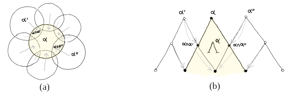
Figure 2.1: $X\subseteq\mathcal{P}(\Omega)$ illustrated as (a) a Venn diagram and (b) a semi-lattice. The colored region represents $\Lambda^{\alpha}=\{\beta^{\prime}\subseteq\alpha\}$ while arrows represent some of the flux contributions to the Gauss formula $\sum_{\beta^{\prime}\in\Lambda^{\alpha}}\delta\varphi_{\beta^{\prime}}=\sum_{\alpha^{\prime}\beta^{\prime}\in d\Lambda^{\alpha}}\varphi_{\alpha^{\prime}\beta^{\prime}}$.

2.2.3   
Systems of Rings and Modules

The category $\{\mathbf{Ring}\}$ of ring systems is similarly defined by restricting to functors $R:X\rightarrow\mathbf{Ring}$. To avoid confusion in applications to come, it will be more convenient to consider cosystems over $X$, i.e. functors $R:X^{op}\rightarrow\mathbf{Ring}$. This subsection, mostly inspired by Kodaira [Kodaira-49], explores the different products and module structures one may generalise from the usual theory with scalar coefficients.

Given a cosystem of rings $R$ over $X$, we give a natural ring structure $\big{(}R^{\bullet}(X),+,\wedge\big{)}$ to its associated cochain complex, by defining the exterior product of a $p$-field $\varphi$ with a $k$-field $\psi$ as the $(p+k)$-field:

$$(\varphi\wedge\psi)_{\alpha\dots\beta\dots\gamma}=\varphi_{\alpha\dots\beta}\cdot\big{[}\psi_{\beta\dots\gamma}\big{]}_{\alpha}$$ (2.24)

where $[\psi_{\beta\dots\gamma}]_{\alpha}$ denotes the image of $\psi_{\beta\dots\gamma}\in R_{\beta}$ in $R_{\alpha}$. The exterior product is compatible with the differential and we have the graded Leibniz rule:

$$d(\varphi\wedge\psi)=d\varphi\wedge\psi+(-1)^{|\varphi|}\;\varphi\wedge d\psi$$ (2.25)

denoting by $|\varphi|$ the degree of $\varphi$, and $\big{(}R^{\bullet}(X),+,\wedge,d\big{)}$ is a differential ring.

There is a natural notion of module over a ring system which makes any ring system a module over itself. The dual notion of comodule will also be of interest to us, they both give a differential module structure to one of the associated complexes.

Definition 2.4.

We call module over $R:X^{op}\rightarrow\mathbf{Ring}$ any cosystem of abelian groups $M:X^{op}\rightarrow\mathbf{Ab}$ such that:

• $M_{\alpha}$ is an $R_{\alpha}$-module for all $\alpha\in X$,

• $[r_{\beta}]_{\alpha}\cdot[m_{\beta}]_{\alpha}=[r_{\beta}\cdot m_{\beta}]_{\alpha}$ for all $\alpha\rightarrow\beta$ in $X$.

where $[m_{\beta}]_{\alpha}$ denotes the image of $m_{\beta}$ in $M_{\alpha}$.

When $M$ is a module over $R$, the cochain complex $M^{\bullet}(X)$ inherits a module structure over $R^{\bullet}(X)$ for the action of $\varphi\in R^{p}(X)$ on $m\in M^{k}(X)$ extending the exterior product:

$$(\varphi\times m)_{\alpha\dots\beta\dots\gamma}=\varphi_{\alpha\dots\beta}\cdot\big{[}m_{\beta\dots\gamma}\big{]}_{\alpha}$$ (2.26)

and the differential $\nabla$ on $M^{\bullet}(X)$ then satisfies the graded module Leibniz rule:

$$\nabla(\varphi\times m)=d\varphi\times m+(-1)^{|\varphi|}\;\varphi\times\nabla m$$ (2.27)

so that $\big{(}M^{\bullet}(X),\nabla\big{)}$ is a differential module over $\big{(}R^{\bullet}(X),d\big{)}$.

Definition 2.5.

We call comodule over $R:X^{op}\rightarrow\mathbf{Ring}$ any system of abelian groups $M:X\rightarrow\mathbf{Ab}$ such that:

• $M_{\alpha}$ is an $R_{\alpha}$-module for all $\alpha\in X$,

• $r_{\beta}\cdot[m_{\alpha}]_{\beta}=[r_{\beta}\cdot m_{\alpha}]_{\beta}$ for all $\alpha\rightarrow\beta$ in $X$.

where $[m_{\alpha}]_{\beta}$ denotes the image of $m_{\alpha}$ in $M_{\beta}$ and $\cdot$ the action of any $R_{\beta}$ such that $\alpha\rightarrow\beta$ on $M_{\alpha}$.

When $M$ is a comodule over $R$, the action of $\varphi\in R^{k}(X)$ on $m\in M_{n}(X)$ is the chain of $M_{n-k}(X)$ given by the interior product:

$$(\varphi\lrcorner\,m)_{\beta\dots\gamma}=\sum_{\alpha^{\prime}\dots\beta}\varphi_{\alpha^{\prime}\dots\beta}\cdot\big{[}m_{\alpha^{\prime}\dots\beta\dots\gamma}\big{]}_{\beta}$$ (2.28)

and by $(\varphi\lrcorner\,m)=0$ when $n<k$. Note that $\lrcorner\,$ actually defines a right action as $(\varphi\wedge\psi)\lrcorner\,m=\psi\lrcorner\,(\varphi\lrcorner\,m)$. The boundary of $M_{\bullet}(X)$ satisfies the graded module Leibniz rule:

$$\delta(\varphi\lrcorner\,\psi)=d\varphi\lrcorner\,\psi+(-1)^{|\varphi|}\;\varphi\lrcorner\,\delta\psi$$ (2.29)

and $\big{(}M_{\bullet}(X),\delta\big{)}$ is a differential module over $\big{(}R^{\bullet}(X),d\big{)}$.

Examples.

1. Consider the constant ring system $\mathbb{Z}$ over $X$, and for every $\alpha\in X$, the $1$-cochain $\lambda^{\alpha}\in\mathbb{Z}^{1}(X)$ defined by:

   $$\lambda^{\alpha}_{\alpha^{\prime}\beta^{\prime}}=\left\{\begin{array}[]{c}1\mathrm{\quad if\quad}\alpha^{\prime}=\alpha\\ 0\mathrm{\quad if\quad}\alpha^{\prime}\neq\alpha\end{array}\right.$$ (2.30)

   An easy computation shows that $d\lambda^{\beta}\in\mathbb{Z}^{2}(X)$ may be written for all $\beta\in X$ as:

   $$d\lambda^{\beta}=\sum_{\alpha\rightarrow\beta}\lambda^{\alpha}\wedge\lambda^{\beta}$$ (2.31)

2. Any cosystem of algebras $A:X^{op}\rightarrow\mathbf{Alg}$ is a comodule over $\mathbb{Z}$. For every $\beta\in X$ we then denote by $i_{\beta}$ the degree $-1$ endomorphism of $A_{\bullet}(X)$ defined by $i_{\beta}(\varphi)=\lambda^{\beta}\lrcorner\,\varphi$. For every $\bar{\gamma}\in N(X)$, if $\beta\not\rightarrow\gamma_{0}$ we have $i_{\beta}(\varphi)_{\bar{\gamma}}=0$ and otherwise:

   $$i_{\beta}(\varphi)_{\bar{\gamma}}=\varphi_{\beta\bar{\gamma}}$$ (2.32)

   The previous example and the graded module Leibniz rule give the following formula:

   $$\delta(i_{\beta}\varphi)=i_{\beta}\Big{(}\sum_{\alpha\rightarrow\beta}i_{\alpha}\varphi\Big{)}-i_{\beta}(\delta\varphi)$$ (2.33)

   which will be very useful in the proof of proposition LABEL:higher-zeta-cocycle.

2.3   
Local Statistics

Localising the statistical structures of section 1, this section restricts the previous constructions to a projective system of sets given by cartesian products $E_{\alpha}=\prod_{i\in\alpha}E_{i}$ of atomic configuration spaces, and focuses on the inductive system $A_{\alpha}=\mathbb{R}^{E_{\alpha}}$ of algebras induced above it.

A fundamental consequence of this hypothesis is the so-called interaction decomposition theorem. It asserts that each algebra of observables splits as a direct sum $A_{\alpha}=\bigoplus_{\beta}Z_{\beta}$, where the interaction vector spaces $Z_{\beta}$ may be chosen consistently over $X$ and play the role of independent generators. This well-known yet subtle result may be given a significant number of proofs and calls for greater generality, but the simple setting we consider allows for a beautiful proof via harmonic analysis.

The main result of this section is the acyclicity of the complex of local observables $A_{\bullet}(X)$. We show that the homology class of $h\in A_{0}(X)$ is completely determined by its global sum $H_{\Omega}=\sum_{\alpha}h_{\alpha}$ in $A_{\Omega}$. In a physical terminology, one would say that two potentials $h$ and $h^{\prime}$ are homologous if and only if they define the same global hamiltonian $H_{\Omega}$.

2.3.1   
Statistical System

From now on, we consider a finite set of atoms $\Omega$ with finite sets of microstates $E_{i}$ for all $i\in\Omega$. The configuration space $E_{\alpha}$ of any region $\alpha\subseteq\Omega$ is defined as:

$$E_{\alpha}=\prod_{i\in\alpha}E_{i}$$ (2.34)

For every $\alpha\supseteq\beta$, we denote the canonical projection by $\pi^{\beta\alpha}:E_{\alpha}\rightarrow E_{\beta}$. Alternatively, one could say that $E:\big{(}\mathcal{P}(\Omega),\supseteq\big{)}\rightarrow\mathbf{Set}$ defines a sheaf of finite sets over the finite topological space $\Omega$.

Given these sets of microstates, local algebras of observables are defined by $A_{\alpha}=\mathbb{R}^{E_{\alpha}}$ and for every $\alpha\supseteq\beta$, the canonical injection $j_{\alpha\beta}:A_{\beta}\rightarrow A_{\alpha}$ is the pull-back of $\pi^{\beta\alpha}$ sending a function on $E_{\beta}$ to its cylindrical extension on $E_{\alpha}$. The multiplicative structure of $E$ is carried to $A$ by:

$$A_{\alpha}=\bigotimes_{i\in\alpha}A_{i}$$ (2.35)

as $A_{\alpha}$ is linearly generated by the Dirac masses $(\delta_{x_{\alpha}})$ on $E_{\alpha}$, which may be written as pure tensors of the form $\delta_{x_{i}}\otimes\dots\otimes\delta_{x_{j}}$, and the extension map $j_{\alpha\beta}$ may then be viewed as the tensor multiplication $1_{\alpha\smallsetminus\beta}\otimes-$ with the unit of $A_{\alpha\smallsetminus\beta}$. Better suited generators $(\chi_{k_{\alpha}})$ will be introduced in the next section.

In the following, we suppose chosen a covering $X\subseteq\mathcal{P}(\Omega)$ closed under intersection, i.e. such that:

$$\alpha\in X\mathrm{\quad and\quad}\beta\in X\quad\Rightarrow\quad\alpha\cap\beta\in X$$ (2.36)

We then restrict $E$ to a system $E:X\rightarrow\mathbf{Set}$ and $A$ to a cosystem $A:X^{op}\rightarrow\mathbf{Alg}$ over $X$. The closure hypothesis is fundamental for the interaction decomposition theorem to hold, it will also be useful for the generalised combinatorics we propose in chapter 3.

Definition 2.6.

We denote by:

• $\big{(}A_{\bullet}(X),\delta\big{)}$ the chain complex of local observables,

• $\big{(}A^{*}_{\bullet}(X),d\big{)}$ the cochain complex of local measures,

• $\Delta_{\bullet}(X)\subseteq A^{*}_{\bullet}(X)$ the convex subspace of local probabilities.

This localisation procedure will lead us to represent the global hamiltonian $H_{\Omega}\in A_{\Omega}$ by a homology class of interaction potentials $(h_{\alpha})\in A_{0}(X)$ satisfying:

$$H_{\Omega}=\sum_{\alpha\in X}h_{\alpha}$$ (2.37)

The global Gibbs state $p_{\Omega}\in\Delta_{\Omega}$ would also be ideally represented by its local marginals $(p_{\alpha})\in\Delta_{0}(X)$ or an approximation of the latter. Marginals of $p_{\Omega}$ are said consistent as $p_{\beta}$ is the marginal of $p_{\alpha}$ for every $\beta\subseteq\alpha$, and the following more general notion of cohomology class in $\Delta_{0}(X)$ will substitute for the global probabilities of $\Delta_{\Omega}$.

Definition 2.7.

The convex subspace $\Gamma(X)$ of consistent local probabilities is defined by:

$$\Gamma(X)=\Delta_{0}(X)\cap\operatorname{Ker}(d)$$ (2.38)

We also denote by $\mathring{\Gamma}(X)$ the space of consistent positive local probabilities.

The image of $\Delta_{\Omega}$ in $\Delta_{0}(X)$ is in general a strict convex polytope of $\Gamma(X)$, as although any consistent $q\in\Gamma(X)$ may always be extended to a global measure $q_{\Omega}\in A^{*}_{\Omega}$, the non-negativity of $q_{\Omega}$ is not insured. This was already noticed by Vorob’ev who first characterised the simplicial complexes $X$ having the property that any consistent family of probabilities in $\Gamma(X)$ may be extended to $\Delta_{\Omega}$. They essentially coincide with the retractable hypergraphs on which we show message-passing algorithms to be exact in chapter 6.

2.3.2   
Interaction Decomposition

For every $\alpha\supseteq\beta$ in $X$, the algebra $A_{\beta}$ is naturally embedded in $A_{\alpha}$. Therefore $A_{\alpha}$ contains observables that may be split as a sum of observables on strict subregions of $\alpha$. We call them boundary observables and write:

$$B_{\alpha}=\sum_{\alpha\supset\beta}A_{\beta}$$ (2.39)

We say that $Z_{\alpha}$ is an interaction subspace of $A_{\alpha}$ if it is a supplement of $B_{\alpha}$. One may then write:

$$A_{\alpha}=Z_{\alpha}\oplus\Big{(}\>\sum_{\alpha\supset\beta}A_{\beta}\>\Big{)}$$ (2.40)

and continue this procedure inductively, which is the content of the interaction decomposition theorem.

Theorem 2.8.

Given an interaction subspace $Z_{\alpha}\subseteq A_{\alpha}$ for every $\alpha\in X$, one has for all $\alpha$:

$$A_{\alpha}=\bigoplus_{\alpha\supseteq\beta}Z_{\beta}$$ (2.41)

It will be useful to consider the following rewording of the theorem. In this point of view, interaction subspaces define a cosystem of vector spaces $Z:X^{op}\rightarrow\mathbf{Vect}$ with trivial maps, embedded in $A$, and we denote by $Z_{0}(X)$ their direct sum viewed as a subspace of $A_{0}(X)$.

Corollary 2.9.

Given a choice of interaction subspaces, we have a projection $P:A_{0}(X)\rightarrow Z_{0}(X)$ given by:

$$P(u)_{\beta}=\sum_{\alpha\supseteq\beta}P^{\beta\alpha}(u_{\alpha})$$ (2.42)

where $P^{\beta\alpha}:A_{\alpha}\rightarrow Z_{\beta}$ is a projection of $A_{\alpha}$ onto $Z_{\beta}$, vanishing on $Z_{\gamma}$ for every $\gamma\neq\beta$.

The theorem asserts that a direct sum decomposition holds for any choice of interaction subspaces. As supplements of boundary observables, they are not defined intrinsically, although unless explicit mention of the opposite, $Z_{\alpha}$ will from now on be assumed orthogonal to $B_{\alpha}$ for the canonical scalar product of $\mathbb{R}^{E_{\alpha}}$. This choice will play a particular role in describing the high temperature limit, see for instance LABEL:T_0_Z and LABEL:transversality-0.

Definition 2.10.

The canonical interaction subspaces $Z_{\alpha}\subseteq A_{\alpha}$ are defined as orthogonal supplements of boundary observables for the canonical scalar product of $A_{\alpha}\simeq\mathbb{R}^{E_{\alpha}}$:

$$Z_{\alpha}=\Big{(}\sum_{\beta\subset\alpha}\operatorname{Im}\big{(}j_{\alpha\beta}\big{)}\Big{)}^{\perp}\quad\Leftrightarrow\quad Z_{\alpha}=\bigcap_{\beta\subset\alpha}\operatorname{Ker}\big{(}\Sigma^{\beta\alpha}\big{)}$$ (2.43)

Instead of proving 2.8 in its generality, inspired by Matǔs, we show how harmonic analysis gives an enlightening perspective on the canonical interaction decomposition. This seems to be the most natural construction of the projections $P^{\beta\alpha}$ and is the one we implemented in javascript.

Chose an ordering of $E_{j}$ for all $j\in\Omega$, so that each $E_{\alpha}$ may be identified with the finite torus:

$$E_{\alpha}\simeq\prod_{j\in\alpha}\frac{\mathbb{Z}}{N_{j}\mathbb{Z}}$$ (2.44)

and consider for every $\alpha\in X$ the complexified algebra of observables $\tilde{A}_{\alpha}=\mathbb{C}^{E_{\alpha}}$. It is a fundamental result of abelian group theory that the spectrum $\hat{E}_{\alpha}=\operatorname{Hom}(E_{\alpha},\mathbb{C}^{*})$ of $E_{\alpha}$ defines an orthormal basis of $\tilde{A}_{\alpha}$ for its canonical hermitian product, where the so-called characters of $\hat{E}_{\alpha}$ are plane waves generating a discrete Fourier transform on $\tilde{A}_{\alpha}$.

By duality, there is a natural injection $\hat{E}_{\beta}\rightarrow\hat{E}_{\alpha}$ by pull-back of the projection $\pi^{\beta\alpha}:E_{\alpha}\rightarrow E_{\beta}$. Consider the subset $\hat{F}_{\alpha}\subseteq\hat{E}_{\alpha}$ of characters defined by:

$$\hat{F}_{\alpha}=\bigcup_{\beta\subset\alpha}\hat{E}_{\beta}$$ (2.45)

It is easily seen that $\hat{F}_{\alpha}$ is an orthonormal basis of the subspace $\tilde{B}_{\alpha}$ of complex boundary observables. Its complement $\hat{G}_{\alpha}$ then provides with an orthonormal basis of the interaction subspace $\tilde{Z}_{\alpha}=\tilde{B}_{\alpha}^{\perp}$. The interaction decomposition theorem here amounts to the observation that $\hat{E}_{\alpha}$ is recovered as the disjoint union:

$$\hat{E}_{\alpha}=\bigsqcup_{\beta\subseteq\alpha}\hat{G}_{\beta}$$ (2.46)

A boundary observable in $\tilde{A}_{\alpha}$ is spanned by plane waves with wave vectors tangent to some $E_{\beta}$ with $\beta\subset\alpha$, and the spectral support of an interaction observable is in the complement of such wave vectors.

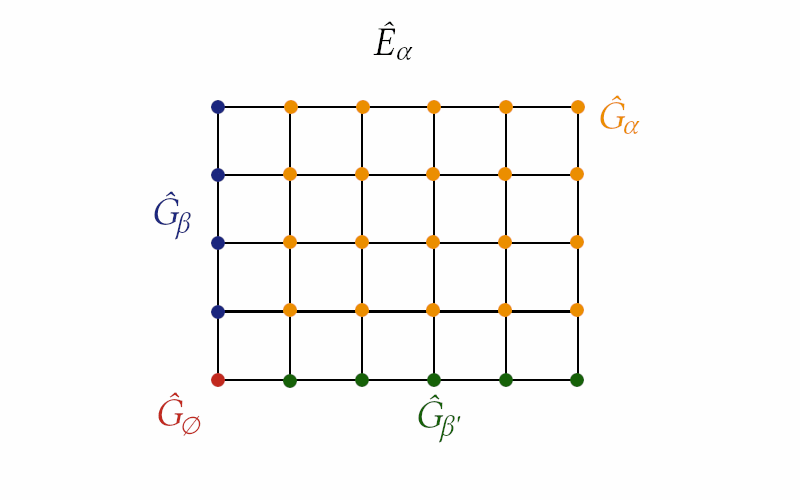
Figure 2.2: Spectral decomposition $\hat{E}_{\alpha}=\bigsqcup_{\beta\subseteq\alpha}\hat{G}_{\beta}$.

More concretely, define for every $k_{\alpha}\in E_{\alpha}$ the character $\chi_{k_{\alpha}}\in\hat{E}_{\alpha}$ by:

$$\chi_{k_{\alpha}}(x_{\alpha})=\operatorname{e}^{i\langle\,k_{\alpha}\,|\,x_{\alpha}\,\rangle}\mathrm{\quad where\quad}\langle\,k_{\alpha}\,|\,x_{\alpha}\,\rangle=\sum_{j\in\alpha}\frac{k_{j}x_{j}}{2\pi N_{j}}$$ (2.47)

The character $\chi_{k_{\beta}}\in\hat{E}_{\beta}$ is extended to $\hat{E}_{\alpha}$ by letting $k_{j}=0$ for $j\notin\beta$. Identifying $\hat{E}_{\alpha}$ with $E_{\alpha}$, the discrete Fourier transform defines a unitary transformation of $\tilde{A}_{\alpha}$. For all $u_{\alpha}\in\tilde{A}_{\alpha}$, write:

$$u_{\alpha}=\sum_{k_{\alpha}\in E_{\alpha}}\hat{u}_{\alpha}(k_{\alpha})\cdot\chi_{k_{\alpha}}$$ (2.48)

The orthogonal projection $P^{\beta\alpha}:\tilde{A}_{\alpha}\rightarrow\tilde{Z}_{\beta}$ is then simply given by selecting only the modes of $G_{\beta}\subseteq E_{\beta}$, complement of $\bigcup_{\beta\subset\gamma}E_{\gamma}$:

$$P^{\beta\alpha}(u_{\alpha})=\sum_{k_{\beta}\in G_{\beta}}\hat{u}_{\alpha}(k_{\beta})\cdot\chi_{k_{\beta}}$$ (2.49)

The real Fourier transform on $A_{\alpha}$ would obviously give a similar explicit construction of real interaction subspaces. This construction appealed to us for both its great conceptual simplicity and ease of implementation. It however strongly relies on the multiplicative structure of the underlying system of sets.

The following proposition gives a more abstract characterisation of interaction subspaces, as other approaches would be necessary for general inductive systems of vector spaces. Note that it is not true in general that the inductive limit splits as a direct sum.

Proposition 2.11.

The inductive limit of $A$ is isomorphic to the direct sum of interaction subspaces:

$$Z_{0}(X)\simeq\operatorname*{colim}_{\alpha\in X}A_{\alpha}$$ (2.50)

Proof.

Let $(V,f)$ denote a cone below $A$ defined by a collection of consistent maps $f_{\beta}:A_{\beta}\rightarrow V$. Identify $(V,f)$ with a map $f:A_{0}(X)\rightarrow V$ and suppose given $\tilde{f}:Z_{0}(X)\rightarrow V$ such that $\tilde{f}\circ P=f$. Then for every $v_{\alpha}\in Z_{\alpha}\subseteq A_{0}(X)$, we have $\tilde{f}(v_{\alpha})=f(v_{\alpha})$. This defines a unique map $\tilde{f}:Z_{0}(X)\rightarrow V$ factorising $f$ through $P$, and $Z_{0}(X)$ satisfies the universal property of the colimit. ∎

The inclusions of each $A_{\alpha}$ into the global algebra $A_{\Omega}$ induce a map $\zeta_{\Omega}:A_{0}(X)\rightarrow A_{\Omega}$ on the direct sum, given by:

$$\zeta_{\Omega}:h\longmapsto\sum_{\alpha\in X}h_{\alpha}$$ (2.51)

We denote by $B_{\Omega}\subseteq A_{\Omega}$ its image. It follows from the previous proposition that we have a universal map from $Z_{0}(X)$ to $B_{\Omega}$, factorising $\zeta_{\Omega}$ through $P$:

$$\bcd A_{0}(X)\rar{P}\drar[swap]$$ (2.52)

&Z0(X)[dashed] BΩ⊆AΩ

Chosing a global interaction subspace to write $A_{\Omega}=Z_{\Omega}\oplus B_{\Omega}$, the interaction decomposition theorem asserts that $A_{\Omega}=Z_{\Omega}\oplus Z_{0}(X)$ so that $Z_{0}(X)$ and $B_{\Omega}$ are isomorphic. This allows for two different representations of the inductive limit, a local one, and a global one.

Proposition 2.12.

The two following maps are equivalent representations of $\operatorname*{colim}A$:

1. $P:A_{0}(X)\longrightarrow Z_{0}(X)$

2. $\zeta_{\Omega}:A_{0}(X)\longrightarrow B_{\Omega}$

2.3.3   
Homology and Cohomology

The global hamiltonian $H_{\Omega}$ of a physical system is typically given as a sum of local interactions:

$$H_{\Omega}=\sum_{\alpha\in X}h_{\alpha}$$ (2.53)

and we will see that $H_{\Omega}=\zeta_{\Omega}(h)$ represents a unique homology class in $A_{0}(X)$. The interaction decomposition theorem is essential to compute the homology of $A_{\bullet}(X)$. We shall first characterise the first homology of $A_{0}(X)$ and the first cohomology of $A^{*}_{0}(X)$, both isomorphic to $Z_{0}(X)$, before proving the acyclicity of the whole complex $A_{\bullet}(X)$.

Theorem 2.13.

The interaction projection $P:A_{0}(X)\rightarrow Z_{0}(X)$ induces an isomorphism in the first homology group of observable fields:

$$\frac{A_{0}(X)}{\delta A_{1}(X)}\simeq Z_{0}(X)$$ (2.54)

Proof.

A Gauss formula on the cone over $\beta\in X$ first ensures that for all $\varphi\in A_{1}(X)$, we have:

$$P(\delta\varphi)_{\beta}=\sum_{\alpha^{\prime}\rightarrow\beta}P^{\beta\alpha^{\prime}}(\delta_{\alpha^{\prime}}\varphi)=\sum_{\alpha^{\prime}\rightarrow\beta}\sum_{\beta^{\prime}\not\rightarrow\beta}P^{\beta\alpha^{\prime}}(\varphi_{\alpha^{\prime}\beta^{\prime}})=0$$ (2.55)

as $P^{\beta\alpha^{\prime}}(A_{\beta^{\prime}})$ is non-zero if and only if $\beta^{\prime}$ contains $\beta$. Hence $P$ vanishes on boundaries and we denote the induced quotient map by $[P]$. Reciprocally, given $u\in A_{0}(X)$ we define $\varphi\in A_{1}(X)$ by $\varphi_{\alpha\beta}=P^{\beta\alpha}(u_{\alpha})$ and consider its boundary:

$$\delta_{\beta}\varphi=\sum_{\alpha^{\prime}\rightarrow\beta}\varphi_{\alpha^{\prime}\beta}-\sum_{\beta\rightarrow\gamma^{\prime}}\varphi_{\beta\gamma^{\prime}}=P(u)_{\beta}-u_{\beta}$$ (2.56)

When $P(u)=0$, the above gives $u=-\delta\varphi$ so that $\operatorname{Ker}(P)=\delta A_{1}(X)$. Hence $[P]$ is injective and induces an isomorphism between $H_{0}(X)=A_{0}(X)/\delta A_{1}(X)$ and its image $Z_{0}(X)$. ∎

It is now a simple consequence of the previous subsection that total energy, viewed as a global observable of $A_{\Omega}$, is a maximal homological invariant of $A_{0}(X)$:

Corollary 2.14.

Two observable fields $h,h^{\prime}\in A_{0}(X)$ are homologous if and only if:

$$\sum_{\alpha\in X}h_{\alpha}=\sum_{\alpha\in X}h^{\prime}_{\alpha}$$ (2.57)

and $\zeta_{\Omega}:A_{0}(X)\rightarrow B_{\Omega}$ induces an isomorphism in homology.

Theorem 2.13 implies that the first cohomology of $A^{*}_{0}(X)$ is also isomorphic to $Z_{0}(X)$ by duality. It is however very instructive to construct the isomorphism explicity, as this representation of consistent measures already involves a fundamental automorphism $\zeta$ of $A_{0}(X)$, the zeta transform, main object of the next chapter. We shall later rewrite theorem 2.15 as:

$$\operatorname{Ker}(d)\>\simeq\>{\color[rgb]{0.62890625,0.125,0.1875}\zeta^{\prime}}\cdot Z_{0}(X)$$ (2.58)

Erratum: The action of $\zeta^{\prime}$ is defined by (2.59) below. Although it requires to rescale the injection of $A_{\beta}$ into $A_{\alpha}$ by volumic factors, it still fits under the definition of zeta transforms given by (3.16). Without the volumic terms, one has $\operatorname{Ker}(\nabla)=\zeta\cdot Z_{0}(X)$ as per (LABEL:T_0_Z), where $\nabla$ is also an adjoint of $\delta$, but where partial integrations have been replaced by conditional expectations for the uniform measure.

Theorem 2.15.

A collection of measures $(q_{\alpha})\in A^{*}_{0}(X)$ is consistent if and only if there exists a collection of interaction potentials $(u_{\alpha})\in Z_{0}(X)$ such that for all $\alpha\in X$:

$$q_{\alpha}=\sum_{\alpha\supseteq\beta}\>{\color[rgb]{0.62890625,0.125,0.1875}\frac{|E_{\beta}|}{|E_{\alpha}|}}\langle\,u_{\beta}\,|\,-\,\rangle_{\alpha}$$ (2.59)

where $\langle\,-\,|\,-\,\rangle_{\alpha}$ denotes the canonical scalar product of $\mathbb{R}^{E_{\alpha}}$.

Proof.

As $\Sigma^{\beta\alpha}$ is the orthogonal projection onto $\mathbb{R}^{E_{\beta}}\subseteq\mathbb{R}^{E_{\alpha}}$ for the canonical scalar product of $\mathbb{R}^{E_{\alpha}}$, we have $\Sigma^{\beta\alpha}(Z_{\gamma})=Z_{\gamma}$ for every $\gamma\subseteq\beta$ and $\Sigma^{\beta\alpha}(Z_{\gamma})=0$ otherwise. Hence for every $q\in A^{*}_{0}(X)$ of the form (2.59) one has:

$$\Sigma^{\beta\alpha}(q_{\alpha})=\sum_{\alpha\supseteq\gamma}\Sigma^{\beta\alpha}\bigg{(}{\color[rgb]{0.62890625,0.125,0.1875}\frac{|E_{\gamma}|}{|E_{\alpha}|}}\>u_{\gamma}\bigg{)}=\sum_{\beta\supseteq\gamma}{\color[rgb]{0.62890625,0.125,0.1875}\frac{|E_{\gamma}|}{|E_{\beta}|}}\>u_{\gamma}=q_{\beta}$$ (2.60)

Reciprocally, given a consistent $q\in A^{*}_{0}(X)$ one may recover $u\in Z_{0}(X)$ by Möbius inversion, see 3.1. It however suffices here to conclude by dimension using theorem 2.13. ∎

Let us now prove the acyclicity of $A_{\bullet}(X)$ by constructing an explicit retraction of $A_{\bullet}(X)$ to $Z_{0}(X)$. For every $\alpha\in X$, we denote by ${\bf z}_{\alpha}$ and ${\bf b}_{\alpha}$ the coherent projectors onto $Z_{\alpha}$ and $B_{\alpha}$, so that:

$$\operatorname{id}_{A_{\alpha}}={\bf z}_{\alpha}\oplus{\bf b}_{\alpha}$$ (2.61)

They induce projectors ${\bf z}$ and ${\bf b}$ onto the subspaces $Z_{\bullet}(X)$ and $B_{\bullet}(X)$ of $A_{\bullet}(X)$.

Denoting by $d$ the adjoint of $\delta$ for the canonical metric of $A_{\bullet}(X)$, consider the homotopy $\eta={\bf z}\circ d\circ{\bf b}$. Explicitly, $\eta:A_{p}(X)\rightarrow A_{p+1}(X)$ acts on $\varphi\in A_{p}(X)$ by:

$$\eta(\varphi)_{\bar{\alpha}\beta}=(-1)^{p+1}\,{\bf z}_{\beta}(\varphi_{\bar{\alpha}})$$ (2.62)

Proposition 2.16.

The map $\eta={\bf z}\,d\,{\bf b}$ defines a homotopy between the identity of $A_{\bullet}(X)$ and the homogeneous extension of the interaction projection $P:A_{\bullet}(X)\rightarrow Z_{0}(X)$:

$$\eta\delta+\delta\eta=1-P$$ (2.63)

Proof.

First, notice that $B_{\bullet}(X)$ is stable under $\delta$ so that ${\bf z}\delta{\bf b}=0$ and $\delta$ splits in the triangular form:

$$\delta={\bf b}\delta{\bf b}+{\bf b}\delta{\bf z}+{\bf z}\delta{\bf z}$$ (2.64)

As $\eta={\bf z}d{\bf b}$, we then have:

$$\delta\eta+\eta\delta=({\bf b}\delta{\bf z})\eta+\eta({\bf b}\delta{\bf z})+{\bf z}(\delta\eta+\eta\delta){\bf b}$$ (2.65)

As maps between $Z_{\bullet}(X)$ and $B_{\bullet}(X)$, the interaction theorem implies that ${\bf b}\delta{\bf z}$ inverts $\eta$ on non-zero degrees. More precisely, for every $p\geq 1$ and $\varphi\in A_{p}(X)$ we have:

$$({\bf b}\delta{\bf z})(\varphi)_{\bar{\beta}}=(-1)^{p}\sum_{\bar{\beta}\supset\gamma^{\prime}}{\bf z}_{\gamma}(\varphi_{\bar{\beta}\gamma^{\prime}})$$ (2.66)

Denoting by ${\bf z}_{0}$ the homogeneous projection onto $Z_{0}(X)$ induced by ${\bf z}$, we may write:

$$({\bf b}\delta{\bf z})\eta={\bf b}\mathrm{\quad and\quad}\eta({\bf b}\delta{\bf z})={\bf z}-{\bf z}_{0}$$ (2.67)

so that $({\bf b}\delta{\bf z})\eta+\eta({\bf b}\delta{\bf z})=1-{\bf z}_{0}$ and it only remains to show that ${\bf z}(\delta\eta+\eta\delta){\bf b}={\bf z}_{0}-P$.

On the zero degree, we have for all $u\in A_{0}(X)$ and $\beta\in X$:

$$({\bf z}\delta\eta)(u)_{\beta}=-\sum_{\alpha^{\prime}\supset\beta}{\bf z}_{\beta}(u_{\alpha^{\prime}})$$ (2.68)

which is precisely ${\bf z}_{0}(u)_{\beta}-P(u)_{\beta}$.

On higher degrees, we have for every $\varphi\in A_{p}(X)$ and $\bar{\beta}\in N_{p}(X)$:

$$({\bf z}\delta\eta)(\varphi)_{\bar{\beta}}=(-1)^{p+1}\sum_{k=0}^{p}(-1)^{k}\sum_{\partial_{k}\bar{\alpha}^{\prime}=\bar{\beta}}{\bf z}_{\alpha^{\prime}_{p+1}}(\varphi_{\alpha^{\prime}_{0}\dots\alpha^{\prime}_{p}})$$ (2.69)

The last summand $k=p+1$ of $\delta\eta(\varphi)_{\bar{\beta}}$ is valued in $B_{\bar{\beta}}$ and truncated by ${\bf z}_{\beta_{p}}$ which enforces $\alpha^{\prime}_{p+1}=\beta_{p}$. On the other hand, we have:

$$(\eta\delta{\bf b})(\varphi)_{\bar{\beta}}={\bf z}_{\beta_{p}}\bigg{(}(-1)^{p}\sum_{k=0}^{p}(-1)^{k}\sum_{\delta_{k}\bar{\beta}^{\prime}=\beta_{0}\dots\beta_{p-1}}{\bf b}_{\beta^{\prime}_{p}}(\varphi_{\bar{\beta}^{\prime}})\bigg{)}$$ (2.70)

Whenever $\beta_{p}\not\subset\beta^{\prime}_{p}$, we have ${\bf z}_{\beta_{p}}\circ{\bf b}_{\beta^{\prime}_{p}}=0$. We may hence assume that $\beta_{p}\subset\beta^{\prime}_{p}$ and let $\bar{\alpha}^{\prime}=\bar{\beta}^{\prime}\beta_{p}$ so that for every $k\leq p$ we have:

$$\delta_{k}\bar{\alpha}^{\prime}=(\delta_{k}\bar{\beta}^{\prime})\beta_{p}=\bar{\beta}$$ (2.71)

Comparing with the above, we see that ${\bf z}\delta\eta+\eta\delta{\bf b}$ vanishes on non-zero degrees, while it is equal to ${\bf z}\delta\eta={\bf z}_{0}-P$ otherwise, which finishes to show that:

$$\delta\eta+\eta\delta=1-{\bf z}_{0}+{\bf z}_{0}-P=1-P$$ (2.72)

∎

Theorem 2.17.

The homology groups of $A_{\bullet}(X)$ are given by:

$$H_{0}(X)\simeq Z_{0}(X)\mathrm{\quad and\quad}H_{n}(X)=0\mathrm{\quad for\quad}n\geq 1$$ (2.73)

Chapter 3 Combinatorics

In this chapter, we review the classical theory of Dirichlet convolution and Möbius inversion. They give algebraic foundations to many combinatorial problems, starting with the so-called inclusion-exclusion principles, generalising the usual formula $|E_{i}\cup E_{j}|=|E_{i}|+|E_{j}|-|E_{i}\cap E_{j}|$. The following structures however really emerged from considerations of number theory.

These methods give insight on the conceptual distinction between intensive and extensive quantities, stemming from the definition internal hamiltonian of a region $\alpha\subseteq\Omega$ as a sum of local interactions:

$$H_{\alpha}=\sum_{\alpha\supseteq\beta}h_{\beta}$$ (3.1)

The extensivity of $H$ may be thought of as a consequence of the quick decay of $h$ on large regions. Möbius inversion will show the relation between $H$ and $h$ to be bijective, a fundamental correspondence which will be written as:

$$H=\zeta\cdot h\quad\Leftrightarrow\quad h=\mu\cdot H$$ (3.2)

In section 1, we start by reviewing the classical theory of incidence algebra. In section 2 we investigate some interesting properties and exhibit a locally cohomological character of the zeta transform $h\mapsto\zeta\cdot h$. In the last and exploratory section, we propose an extension of $\zeta$ and $\mu$ as two reciprocal endomorphisms on the whole complex of observable fields $A_{\bullet}(X)$. This extension of $\zeta$ to higher degrees is done consistently with the local cocyle properties satisfied on the zero degree, while the degree one Möbius transform will allow for various enhancements of the belief propagation algorithm.

3.1   
Dirichlet Convolution

The convolution product on the set of arithmetic functions $f:\mathbb{N}^{*}\rightarrow\mathbb{C}$ was first introduced by Dirichlet in 1837 to prove his theorem on arithmetic progressions. Relying on the partial order structure of $\mathbb{N}^{*}$ induced by divisibility, it is given by:

$$(f*g)(n)=\sum_{d|n}f(d)\,g(n/d)$$ (3.3)

A meromorphic function $\hat{f}$ may be associated to every arithmetic function $f$ of subpolynomial growth by analytic extension of its Dirichlet generating series, defined for all $s\in\mathbb{C}$ such that ${\rm Re}(s)$ is large enough by:

$$\hat{f}(s)=\sum_{n\in\mathbb{N}^{*}}\frac{f(n)}{n^{s}}$$ (3.4)

The assignment $f\mapsto\hat{f}$ interlaces Dirichlet convolution with the usual product on $\mathbb{C}$ and we have for every arithmetic functions $f$ and $g$:

$$\widehat{f*g}=\hat{f}\cdot\hat{g}$$ (3.5)

The Riemann zeta function $\hat{\zeta}$ extends the generating series of the arithmetic function $\zeta$, defined by $\zeta(n)=1$ for all $n\in\mathbb{N}^{*}$. The classical Möbius inversion formula states that $\zeta$ has an inverse for $*$ given by $\mu(n)=(-1)^{k}$ if $n$ is the product of $k$ distinct primes, and zero otherwise. This in turn yields the coefficients of the generating series of $\hat{\mu}=1/\hat{\zeta}$.

Dirichlet convolution and Möbius inversion formulas were then studied in more general contexts, notably by Fréchet, and a fundamental and seminal reference on the subject is the general treatment of Möbius functions given by Rota in [Rota-64]. Dirichlet convolution may not only be defined on a locally finite partial order but on any locally finite category. We however restrict to the former and refer the interested reader to [Leinster-08] for greater generality.

3.1.1   
Incidence Ring

Given a locally finite partially ordered set $X$ and a unital ring $R$, let us denote by $R_{1}(X)$ the $R$-module of $R$-valued functions on the set $N_{1}X$ of $1$-chains in $X$:

$$R_{1}(X)=\big{\{}\,\varphi:X\times X\rightarrow R\;|\;\alpha\not\rightarrow\beta\Rightarrow\varphi_{\alpha\beta}=0\,\big{\}}=R^{N_{1}X}$$ (3.6)

It is equipped with the Dirichlet convolution product $*$ defined for every $\varphi,\psi\in R_{1}(X)$ by:

$$(\varphi*\psi)_{\alpha\gamma}=\sum_{\alpha\rightarrow\beta^{\prime}\rightarrow\gamma}\varphi_{\alpha\beta^{\prime}}\cdot\psi_{\beta^{\prime}\gamma}$$ (3.7)

This product is associative. It has a unit ${\bf 1}$, which is the Kronecker symbol defined by ${\bf 1}_{\alpha\alpha}=1$ and ${\bf 1}_{\alpha\beta}=0$ if $\alpha\neq\beta$.

The unital ring $\big{(}R_{1}(X),+,*\big{)}$ is called the incidence ring of $X$, or incidence algebra when $R$ is a field. Combinatorics are however mostly interested with relative integers and it is remarkable that Möbius inversion can be carried out on $\mathbb{Z}$.

3.1.2   
Incidence Modules

Let $M$ denote a module on $R$, and denote by $M_{1}(X)$ the space of $M$-valued functions on $N_{1}X$. Then $M_{1}(X)$ is a module on the incidence ring $R_{1}(X)$ for the left action defined for $m\in M_{1}(X)$ by:

$$(\varphi\cdot m)_{\alpha\gamma}=\sum_{\alpha\rightarrow\beta^{\prime}\rightarrow\gamma}\varphi_{\alpha\beta^{\prime}}\cdot m_{\beta^{\prime}\gamma}$$ (3.8)

when $M$ is a left $R$-module, and symetrically, for the right action:

$$(m\cdot\psi)_{\alpha\gamma}=\sum_{\alpha\rightarrow\beta^{\prime}\rightarrow\gamma}m_{\alpha\beta^{\prime}}\cdot\psi_{\beta^{\prime}\gamma}$$ (3.9)

when $M$ is a right $R$-module.

Let us now denote by $M_{0}(X)$ the space of $M$-valued functions on $X$. It is also equipped with a left action of $R_{1}(X)$ defined for every $n\in M_{0}(X)$ by:

$$(\varphi\cdot n)_{\alpha}=\sum_{\alpha\rightarrow\beta^{\prime}}\varphi_{\alpha\beta^{\prime}}\cdot n_{\beta^{\prime}}$$ (3.10)

when $M$ is a left module, and otherwise with the right action:

$$(n\cdot\psi)_{\beta}=\sum_{\alpha^{\prime}\rightarrow\beta}n_{\alpha^{\prime}}\cdot\psi_{\alpha^{\prime}\beta}$$ (3.11)

Following Rota, one may relate these two actions and append to $X$ initial and terminal elements $0$ and $1$ when necessary, defining a possibly larger poset $\bar{X}$. To $m\in M_{1}(X)$ associate $n\in M_{0}(X)$ by $n_{\alpha}=m_{\alpha 1}$. This interlaces the two left actions of $R_{1}(\bar{X})$ on when $M$ is a left module. Similarly, letting $n_{\beta}=m_{0\beta}$ interlaces the two right actions.

Notice that when $M=R=\mathbb{R}$, the vector spaces $R_{1}(X)$ and $\mathbb{R}_{0}(X)$ have a canonical scalar product for which the left and right actions define adjoint endomorphisms.

3.1.3   
Systems

Given a cosystem $R:X^{op}\rightarrow\mathbf{Ring}$, we may similarly equip the space of upper $1$-fields $\mathbb{R}^{1}(X)$ with a convolution product. There is a ring morphism $R_{\alpha}\leftarrow R_{\beta}$ for every $\alpha\rightarrow\beta$ in $X$, and for $r_{\beta}\in R_{\beta}$ we denote by $[r_{\beta}]_{\alpha}$ its image in $R_{\alpha}$. Then for $\varphi,\psi\in R_{1}(X)$, let:

$$(\varphi*\psi)_{\alpha\gamma}=\sum_{\alpha\rightarrow\beta^{\prime}\rightarrow\gamma}\varphi_{\alpha\beta^{\prime}}\cdot[\psi_{\beta^{\prime}\gamma}]_{\alpha}$$ (3.12)

By duality, we may similarly define the convolution product $*$ on the space of lower fields $R_{1}(X)$ when $R:X\rightarrow\mathbf{Ring}$ is a system of rings.

When $M:X^{op}\rightarrow\mathbf{Ring}$ is a module over the cosystem $R$, we may extend the left action of $R^{1}(X)$ on the space of upper $1$-fields $M^{1}(X)$. We have a morphism $M_{\alpha}\leftarrow M_{\beta}$ for every $\alpha\rightarrow\beta$ in $X$, and for every $m_{\beta}\in M_{\beta}$, we still denote by $[m_{\beta}]_{\alpha}$ its image in $M_{\alpha}$. The action is then given by:

$$(\varphi\cdot\psi)_{\alpha\gamma}=\sum_{\alpha\rightarrow\beta^{\prime}\rightarrow\gamma}\varphi_{\alpha\beta^{\prime}}\cdot[m_{\beta^{\prime}\gamma}]_{\alpha}$$ (3.13)

And a left action of $R^{1}(X)$ can similarly be defined on $M_{0}(X)$ by:

$$(\varphi\cdot m)_{\alpha}=\sum_{\alpha\rightarrow\beta^{\prime}}\varphi_{\alpha\beta^{\prime}}\cdot[m_{\beta^{\prime}}]_{\alpha}$$ (3.14)

The action of $\mathbb{Z}_{1}(X)$ on the module $A_{0}(X)$ of observable fields, falls into this case. It is the main example we shall be interested in, before considering functors $M$ assigning to each $M_{\alpha}$ the space of functionals on $A_{0}(\Lambda^{\alpha})$ or on the set $\Sigma_{\alpha}$ of states of $A_{\alpha}$.

If $R$ is a fixed ring, then $R^{1}(X)=R_{1}(X)$ has a natural action on the space of lower fields $M_{1}(X)$:

$$(\varphi\cdot m)_{\alpha\gamma}=\sum_{\alpha\rightarrow\beta^{\prime}}\varphi_{\alpha\beta^{\prime}}\cdot m_{\beta^{\prime}\gamma}$$ (3.15)

Although functoriality of $M$ does not appear, this case is worth mentioning as it covers for instance the action of $\mathbb{Z}_{1}(X)$ on $A_{1}(X)$.

Dual constructions take place when $M$ is a covariant functor. In particular, this is the case when $M=A^{*}$ is the module of linear forms on observables, and the right action of $\mathbb{Z}_{1}(X)$ on $A^{*}_{0}(X)$ is the adjoint of its left action on $A_{0}(X)$.

3.2   
Properties of the Zeta Transform

The zeta function $\zeta\in\mathbb{Z}_{1}(X)$ is defined by $\zeta_{\alpha\beta}=1$ for all $\alpha\rightarrow\beta$ in $X$. Given a cosystem of abelian groups $M:X^{op}\rightarrow\mathbf{Ab}$, the left action of $\zeta$ on $M_{0}(X)$ is given by:

$$(\zeta\cdot f)_{\alpha}=\sum_{\alpha\rightarrow\beta}[f_{\beta}]_{\alpha}$$ (3.16)

This section exposes elementary properties of the endomorphism thus defined on $M_{0}(X)$. The first one, bijectivity, is given by the classical Möbius inversion formulas. The next one, locality, is also significant however obvious it is. As an easy consequence of the previous chapter, we then introduce a local cocycle property satisfied by the zeta transform.

3.2.1   
Möbius Inversion

The fundamental theorem of Möbius inversion states that $\zeta$ has an inverse $\mu\in\mathbb{Z}_{1}(X)$ for Dirichlet convolution, it naturally implies the bijectivity of the zeta transform on any module.

Theorem 3.1 (Möbius - Rota).

The inverse of $\zeta\in\mathbb{Z}_{1}(X)$ is the Möbius function $\mu\in\mathbb{Z}_{1}(X)$:

$$\mu=\sum_{k\geq 0}(-1)^{k}(\zeta-{\bf 1})^{k}$$ (3.17)

Proof.

The $n$-th power of $\zeta$ for $*$ counts the number of $n$-chains between any two elements $\alpha,\beta\in X$:

$$\zeta^{n}_{\alpha\beta}=\sum_{\alpha=\alpha_{0}\rightarrow\dots\rightarrow\alpha_{n}=\beta}1$$ (3.18)

and $(\zeta-{\bf 1})^{n}_{\alpha\beta}$ similarly counts the number of non-degenerate $n$-chains from $\alpha$ to $\beta$. Because $X$ is locally finite, there exists $N$ such that $(\zeta-{\bf 1})^{N}_{\alpha\beta}=0$ and $\zeta={\bf 1}+(\zeta-{\bf 1})$ is invertible. ∎

Note that more practical identities arise from the relations $\mu*\zeta=\zeta*\mu={\bf 1}$, allowing to compute the values of $\mu$ inductively. Starting from $\mu_{\alpha\alpha}=1$, one may for instance iterate over $\gamma$ under $\alpha$:

$$\mu_{\alpha\gamma}=1-\sum_{\alpha\geq\beta^{\prime}>\gamma}\mu_{\alpha\beta^{\prime}}$$ (3.19)

The Möbius function $\mu$ is closely related to diverse inclusion-exclusion principles. Consider for example the problem of finding a collection of integers $(c_{\alpha})\in\mathbb{Z}_{0}(X)$ such that for all $\beta\in X$:

$$\sum_{\alpha^{\prime}\rightarrow\beta}c_{\alpha^{\prime}}=1$$ (3.20)

One may compute these coefficients inductively starting from maximal cells. Note that this expression involves the right action of $\zeta$, and as by Möbius inversion $c\cdot\zeta=1$ is equivalent to $c=1\cdot\mu$ we have:

$$c_{\beta}=\sum_{\alpha^{\prime}\rightarrow\beta}\mu_{\alpha^{\prime}\beta}$$ (3.21)

We call $c=1\cdot\mu$ and $\bar{c}=\mu\cdot 1$ the right and left Möbius numbers.

Given $X\subseteq\tilde{X}$, let us say that $X$ is full if for all $\alpha\in X$, every $\beta\in\tilde{X}$ such that $\beta\subseteq\alpha$ is also in $X$.

Proposition 3.2.

If $X$ is full in $\tilde{X}$, then the restriction of the Möbius function of $\tilde{X}$ to $X$ is the Möbius function of $X$.

Proposition 3.3.

If $\tilde{X}=\{\Omega\}\sqcup X$ completes $X$ with an initial element $\Omega$ and $\tilde{\mu}\in\mathbb{Z}_{1}(\tilde{X})$ denotes the Möbius function on $\tilde{X}$, then for every $\beta\in X$ we have $c_{\beta}=-\tilde{\mu}_{\Omega\beta}$.

Proof.

The Möbius inversion formula in $\tilde{X}$ between $\Omega$ and $\beta\in X$ gives:

$$\sum_{\Omega\rightarrow\alpha\rightarrow\beta}\tilde{\mu}_{\alpha\beta}=\tilde{\mu}_{\Omega\beta}+\sum_{\alpha\rightarrow\beta}\mu_{\alpha\beta}=\tilde{\mu}_{\Omega\beta}+c_{\beta}=0$$ (3.22)

∎

Examples.

1. Let $X=\mathbb{N}$ denote the standard total order of integers. The Möbius function is given by $\mu_{\alpha\alpha}=1$ and $\mu_{\alpha\beta}=-1$ if $\beta=\alpha+1$, zero otherwise. We recover the classical finite differences formula:

   $$U_{\alpha}=\sum_{\beta=0}^{\alpha}u_{\beta}\quad\Leftrightarrow\quad u_{\alpha}=U_{\alpha}-U_{\alpha-1}$$ (3.23)

   which is the discrete version of the fundamental theorem of calculus.

2. Let $X=\mathcal{P}(\Omega)$ for a finite set $\Omega$ and denote by $|\alpha|$ the cardinal of $\alpha\subseteq\Omega$. The Möbius function is then given by:

   $$\mu_{\alpha\beta}=(-1)^{|\alpha|-|\beta|}$$ (3.24)

   Suppose given now for each $i\in\Omega$ a measurable subset ${\cal A}_{i}$ of some probability space, relate to:

   $$\mathbb{P}(\cup_{i\in\alpha}{\cal A}_{i})=\sum_{\beta\subseteq\alpha}(-1)^{|\beta|}\mathbb{P}(\cap_{j\in\beta}{\cal A}_{j})$$ (3.25)

3. Total interaction$P^{\beta\alpha}$ and marginal projections $\Sigma^{\beta\alpha}$.

   $$\Sigma^{\beta\alpha}=\sum_{\beta\rightarrow\gamma^{\prime}}P^{\gamma^{\prime}\alpha}\quad\Leftrightarrow\quad P^{\beta\alpha}=\sum_{\beta\rightarrow\gamma^{\prime}}\mu_{\beta\gamma^{\prime}}\cdot\Sigma^{\gamma^{\prime}\alpha}$$ (3.26)

   This is a property of the canonical metric and the marginal projections, beware that in general:

   $$\mathbb{E}^{\beta\alpha}\neq\sum_{\beta\rightarrow\gamma^{\prime}}P^{\gamma^{\prime}\alpha}$$ (3.27)

   as $\bigoplus_{\gamma\not\in\Lambda^{\beta}}Z_{\gamma}$ might not be the orthogonal to $A_{\beta}$ in $A_{\alpha}$.

3.2.2   
Locality

For every $\alpha\in X$, we denote by $\Lambda^{\alpha}$ the cone under $\alpha$ consisting of those $\beta\in X$ such that $\alpha\rightarrow\beta$. As subset of $X$, there is a natural restriction map:

$${\rm r}_{\alpha}:M_{0}(X)\longrightarrow M_{0}(\Lambda^{\alpha})$$ (3.28)

For every $f\in M_{0}(X)$ the value of $(\zeta\cdot f)_{\alpha}$ only depends on the values $f_{\beta}$ for $\alpha\rightarrow\beta$. In other words, $\zeta$ commutes with the restriction to $\Lambda^{\alpha}$ and we have ${\rm r}_{\alpha}\circ\zeta=\zeta\circ{\rm r}_{\alpha}$.

$$\bcd M_{0}(X)\rar{{\rm r}_{\alpha}}\dar[swap]$$ (3.29)

&M0(Λα)ζ M0(X)[swap]rαM0(Λα)

This locality property comes from the form of the action of $\mathbb{Z}_{1}(X)$ on $M_{0}(X)$ and is absolutely not specific to $\zeta$. Such local endomorphisms preserve the sheaf structure of $M_{0}(X)$.

Denoting by $i_{\alpha}:M_{0}(X)\rightarrow M_{\alpha}$ the evaluation on $\alpha$, a consequence of the locality of $\zeta$ is that we may factorise $i_{\alpha}\circ\zeta$ through ${\rm r}_{\alpha}$:

$$\bcd M_{0}(X)\rar{{\rm r}_{\alpha}}\drar[swap]$$ (3.30)

&M0(