Prediction of possible $DK_{1}$ bound states

Abstract

Stimulated by recent experimental observation of $X_{1}(2900)$ just below the $\bar{D}_{1}K$ threshold, we extend our previous study of $\bar{D}_{1}D$ S-wave bound state by vector meson exchange to $\bar{D}_{1}K$ system as well as similar $\bar{D}K_{1}$, $D_{1}K$ and $DK_{1}$ systems to look for possible bound states. We find that the potential of $DK_{1}$ is attractive and strong enough to form bound states with mass around 3110 MeV for $DK_{1}(1270)$ and 3240 MeV for $DK_{1}(1400)$. $D_{1}K$ is also attractive but weaker, hardly enough to form bound states. While $\bar{D}K_{1}$ becomes further less attractive, the potential between $\bar{D}_{1}K$ is the weakest, definitely too weak to form any bound state, which excludes the recently observed $X_{1}(2900)$ to be a $\bar{D}_{1}K$ bound state. We also give the decay properties of the predicted $DK_{1}$ bound states.

I Introduction

Two new open flavor states were recently reported by LHCb collaboration Aaij et al. (2020) in the $D^{-}K^{+}$ final state in $B^{+}\rightarrow D^{+}D^{-}K^{+}$ with statistical significance much larger than 5$\sigma$. The fitted masses and widths are

$$X_{0}(2900): M=2866.3\pm 6.5\pm 2.0\mathrm{MeV}/\mathrm{c}^{2}$$

$$\Gamma=57.2\pm 12.2\pm 4.1\mathrm{MeV}/\mathrm{c}^{2}$$

$$X_{1}(2900): M=2904.1\pm 4.8\pm 1.3\mathrm{MeV}/\mathrm{c}^{2}$$

$$\Gamma=110.3\pm 10.7\pm 4.3\mathrm{MeV}/\mathrm{c}^{2}$$

with corresponding quantum numbers of $J^{P}=0^{+}$ and $1^{-}$, respectively. They are very interesting and of great importance since if confirmed to be real resonances instead of kinetic effects, each of them consists of at least four (anti)quarks which are beyond the conventional quark model. Up to now dozens of works have made efforts to understand these two states Karliner and Rosner (2020); He et al. (2020); Zhang (2021); Wang (2020); Lü et al. (2020); Chen et al. (2020); Hu et al. (2021); Liu et al. (2020a); He and Chen (2020); Huang et al. (2020); Xue et al. (2021); Molina and Oset (2020); Agaev et al. (2020); He and Chen (2020); Liu et al. (2020b); Burns and Swanson (2021a); Albuquerque et al. (2021); Chen et al. (2021); Mutuk (2021); Burns and Swanson (2021b). On one hand, $X_{0}(2900)$ is explained as a $cs\bar{u}\bar{d}$ compact tetraquark Karliner and Rosner (2020); He et al. (2020); Zhang (2021); Wang (2020); Wang et al. (2021), but this explanation is disfavored by explicit calculation of spectra using extended quark model Lü et al. (2020). On the other hand, $X_{0}(2900)$ is also regarded as a molecule of $\bar{D}^{*}K^{*}$ Chen et al. (2020); Hu et al. (2021); Liu et al. (2020a); Huang et al. (2020); He and Chen (2020); Molina and Oset (2020); Agaev et al. (2020); Mutuk (2021); Xiao et al. (2021). It worth mentioning that in Ref. Molina et al. (2010) a bound state of $D^{*}\bar{K}^{*}$ with $I=0,\ J^{P}=0^{+}$ whose mass is close to that of $X_{0}(2900)$ is predicted. Similarly, $X_{1}(2900)$ is explained as a compact tetraquark Chen et al. (2020); He et al. (2020); Xue et al. (2021); Molina and Oset (2020); Agaev et al. (2020); Mutuk (2021); Agaev et al. (2021), a $\bar{D}_{1}K$ virtual state He and Chen (2020) or a $\bar{D}_{1}K$ bound state Tan and Ping (2020); Qi et al. (2021). Besides, these exotic signals in LHCb’s observation are explained as kinetic effect, namely, triangle singularity in Refs.Liu et al. (2020b); Burns and Swanson (2021a). The conflicts among these different interpretations suggest that more experimental results are needed to pin down the nature of these states.

Since the discovery of $\chi_{c0}(3872)$ Choi et al. (2003) in 2003, plenty of exotic states or candidates are observed experimentally, many of which are close to certain hadron pair thresholds and are explained as hadronic molecules Guo et al. (2018). Note that $X_{0}(2900)$ and $X_{1}(2900)$ are about 30 and 10 MeV below $\bar{D}^{*}K^{*}$ and $\bar{D}_{1}K$ threshold, respectively. Therefore, it is natural to explore the existence of $\bar{D}^{*}K^{*}$ and $\bar{D}_{1}K$ molecules, which have already been explored in Refs. Chen et al. (2020); Hu et al. (2021); Liu et al. (2020a); He and Chen (2020); Mutuk (2021) with different methods. In our previous works Dong et al. (2020, 2021) we applied the meson exchange model to $DD_{1}$ system to investigate the molecular explanation of $Y(4260)$ and an exotic $1^{-+}$ molecule has been predicted. We now extend the study to $DK_{1}$ and $D_{1}K$ systems to look for possible bound states.

Actually, the states related to $c\bar{s}$ have attract attention since the discovery of $D_{s0}^{*}(2317)$ Aubert et al. (2003); Besson et al. (2003) which is explained as a $DK$ molecule. See Ref. Chen et al. (2017) for a review on the spectrum of $D_{sJ}$ mesons. Besides the plenty of phenomenological researches, the direct and indirect calculations on lattice Liu et al. (2013); Martínez Torres et al. (2015); Bali et al. (2017); Cheung et al. (2021) provide strong evidences favoring the molecular explanation of $D_{s0}^{*}(2317)$, which almost settles the dispute on the nature of $D_{s0}^{*}(2317)$. Based on this assumption, more kaonic and charmed meson molecules, including $D_{1}K$, are predicted, which are possible interpretations of some observed $D_{sJ}$ states Guo and Meissner (2011).

This work is organized as follows. In section II, the potentials of different systems are derived and the binding energy of possible bound states are calculated. In section III, the decay patterns of the predicted bound states are estimated. A brief summary is given in section IV.

II The potentials and possible bound states

Figure 1: Feynman diagrams for vector meson exchange between $DK_{1}$, $\bar{D}K_{1}$, $D_{1}K$ and $\bar{D}_{1}K$.

The meson exchanged interactions for $DK_{1}$ and $D_{1}K$ systems are illustrated in Fig.(1) respectively. The relevant Lagrangians are collected in the following.

The couplings of heavy mesons and light vector meson can be described by the effective Lagrangians with the hidden gauge symmetry Casalbuoni et al. (1997). For $D$ and $D_{1}$ mesons, the Lagrangians read explicitly Ding (2009)

$$\mathcal{L}_{\mathrm{DDV}} =\frac{i\beta g_{V}}{\sqrt{2}}\left(\mathrm{D}_{b}\stackrel{{\scriptstyle\leftrightarrow}}{{\partial}}_{\mu}\mathrm{D}_{a}^{\dagger}-\overline{\mathrm{D}}_{a}\stackrel{{\scriptstyle\leftrightarrow}}{{\partial}}_{\mu}\overline{\mathrm{D}}_{b}^{\dagger}\right)V_{ba}^{\mu}$$ (1)

$$\mathcal{L}_{\mathrm{D}_{1}\mathrm{D}_{1}V} =\frac{i\beta_{2}g_{V}}{\sqrt{2}}\left(\mathrm{D}_{1b}^{\nu}\stackrel{{\scriptstyle\leftrightarrow}}{{\partial}}_{\mu}\mathrm{D}_{1a\nu}^{\dagger}-\overline{\mathrm{D}}_{1a\nu}\stackrel{{\scriptstyle\leftrightarrow}}{{\partial}}_{\mu}\overline{\mathrm{D}}_{1b}^{\nu\dagger}\right)V_{ba}^{\mu}$$ (2)

where

$$D_{(1)} =(D_{(1)}^{0},D_{(1)}^{+},D_{s(1)}^{+})$$ (3)

$$V =\left(\begin{array}[]{ccc}{\frac{1}{\sqrt{2}}\rho^{0}+\frac{1}{\sqrt{2}}}\omega&{\rho^{+}}&{K^{*+}}\\ {\rho^{-}}&{-\frac{1}{\sqrt{2}}\rho^{0}+\frac{1}{\sqrt{2}}\omega}&{K^{*0}}\\ {K^{*-}}&{\bar{K}^{*0}}&{\phi}\end{array}\right)$$ (7)

with $g_{V}=5.8$ Bando et al. (1988) and $\beta=0.9$ Isola et al. (2003). As analysed in Ref. Dong et al. (2020), $\beta_{2}\approx-\beta$. Here we have taken the ideal mixing between $\omega_{0}$ and $\omega_{8}$.

In the light meson sector, the nature of $K_{1}(1270)$ and $K_{1}(1400)$ that both are conventional $q\bar{q}$ mesons Burakovsky and Goldman (1997); Suzuki (1993); Cheng (2003); Yang (2011); Hatanaka and Yang (2008); Tayduganov et al. (2012); Divotgey et al. (2013); Zhang et al. (2018) or $K_{1}(1270)$ is a dynamically generated resonance with possible two pole structure  Roca et al. (2005); Geng et al. (2007); Wang et al. (2019), is still controversial and in this work we adopt the former one. Due to the mass difference between $u/d$ and $s$ quarks, the axialvector $K_{1A}$ (${}^{3}P_{1}$ state) and pseudovector $K_{1B}$ (${}^{1}P_{1}$ state) mix and generate the two physical resonances $K_{1}(1270)$ and $K_{1}(1400)$. Following Ref. Divotgey et al. (2013) the mixing is parameterized as

$$\left(\begin{array}[]{cc}{\left|K_{1}(1270)\right\rangle}\\ {\left|K_{1}(1400)\right\rangle}\end{array}\right)=\left(\begin{array}[]{cc}{\cos\phi}&{-i\sin\phi}\\ {-i\sin\phi}&{\cos\phi}\end{array}\right)\left(\begin{array}[]{c}{\left|K_{1A}\right\rangle}\\ {\left|K_{1B}\right\rangle}\end{array}\right)$$ (14)

with the mixing angle $\phi$ determined to be $(56.4\pm 4.3)^{\circ}$.

From chiral perturbation theory, the pseudoscalar-pseudoscalar-vector coupling reads

$$\mathcal{L}_{\rm{PPV}} =i\sqrt{2}\,G_{\rm V}\,{\rm{Tr}}\left([\partial_{\mu}P,P]V^{\mu}\right).$$ (15)

and analogously,

$$\mathcal{L}_{\rm{AAV}} =i\sqrt{2}\,G_{\rm V}^{\prime}\,{\rm{Tr}}\left([\partial_{\mu}A^{\nu},A_{\nu}]V^{\mu}\right)$$ (16)

$$\mathcal{L}_{\rm{BBV}} =i\sqrt{2}\,G_{\rm V}^{\prime}\,{\rm{Tr}}\left([\partial_{\mu}B^{\nu},B_{\nu}]V^{\mu}\right)$$ (17)

with

$$P=\left(\begin{array}[]{ccc}{\frac{1}{\sqrt{2}}\pi^{0}+\frac{1}{\sqrt{6}}\eta_{8}}&{\pi^{+}}&{K^{+}}\\ {\pi^{-}}&{-\frac{1}{\sqrt{2}}\pi^{0}+\frac{1}{\sqrt{6}}\eta_{8}}&{K^{0}}\\ {K^{-}}&{\bar{K}^{0}}&{-\frac{2}{\sqrt{6}}\eta_{8}}\end{array}\right),$$ (21)

$$A(B)=\left(\begin{array}[]{ccc}{*}&{*}&{K_{1A(B)}^{+}}\\ {*}&{*}&{K_{1A(B)}^{0}}\\ {K_{1A(B)}^{-}}&{\bar{K}_{1A(B)}^{0}}&*\end{array}\right).$$ (25)

The coupling constant $G_{\rm V}\approx 3.0$ was estimated from the decay width of $\rho\to\pi\pi$ Zhang et al. (2006) and we adopt the approximation $G^{\prime}_{\rm V}\approx-G_{\rm V}$. Note that the irrelevant axialvector and pseudovector states are not shown explicitly in the corresponding multiplet and represented by “*”. Expanding Eq.(15) we obtain the couplings between $KKV$,

$$\mathcal{L}_{\rho KK} =iG_{V}\left[\bar{K}\vec{\tau}\left(\partial_{\mu}K\right)-\left(\partial_{\mu}\bar{K}\right)\vec{\tau}K\right]\cdot\vec{\rho}^{\mu},$$ (26)

$$\mathcal{L}_{\omega KK} =iG_{V}\left[\bar{K}\left(\partial_{\mu}K\right)-\left(\partial_{\mu}\bar{K}\right)K\right]\omega^{\mu},$$ (27)

$$\mathcal{L}_{\phi KK} =-\sqrt{2}iG_{V}\left[\bar{K}\left(\partial_{\mu}K\right)-\left(\partial_{\mu}\bar{K}\right)K\right]\phi^{\mu}$$ (28)

with

$$K =\left(\begin{array}[]{c}{K^{+}}\\ {K^{0}}\end{array}\right),\bar{K}=\left(K^{-},\bar{K}^{0}\right),$$ (31)

$$\vec{\rho} =\left(\frac{\rho^{+}+\rho^{-}}{\sqrt{2}},\frac{\rho^{-}-\rho^{+}}{i\sqrt{2}},\rho^{0}\right)$$ (32)

and $\vec{\tau}$ the Pauli matrices in isospin space. The coupling between $K_{1}K_{1}V$ has the same form as Eqs.(26,27,28).

The potentials in momentum space are

$$\tilde{V}({\bf q})=f_{\mathrm{I}}g_{D}g_{K}\frac{1}{|{\bf q}|^{2}+m_{\rm V}^{2}}$$ (33)

where the involved constants are listed in Tab.(1). The relative signs of $g_{D}$ and $g_{K}$ for different systems are determined by the following facts. It is easy to see that the vector meson exchange yields an attractive potential of $D\bar{D}$ system and thus $DK$ system is also attractive since $c$ and $s$ quarks are spectators during the interaction. These are consistent with the potentials from the Weinberg-Tomozawa term Weinberg (1966); Tomozawa (1966). Therefore, $D\bar{D}_{1}$, $DK_{1}$ and $D_{1}K$ should all have attractive interactions Guo and Meissner (2011), which in turn fixes the potentials of all other related systems. These determined signs are in agreement with the fact that the $Y(4260)$ contains sizeable components of $D\bar{D}_{1}$ bound state Wang et al. (2013); Chen et al. (2019).

Table 1: Constants in Eq.(33) for different systems. $f_{I}$ is the isospin factors with $I=0$ or 1. $\rho$ and $\omega$ are the exchanged particles. $g_{D/K}$ stands for the $D_{(1)}D_{(1)}V/K_{(1)}K_{(1)}V$ coupling constants.

	$f_{0}$		$f_{1}$		$g_{D}$	$g_{K}$
	$\rho$	$\omega$	$\rho$	$\omega$
$DK_{1}$	3	1	-1	1	$\beta g_{V}/{\sqrt{2}}$	$-G_{V}$
$D\bar{K}_{1}$	-3	1	1	1	$\beta g_{V}/{\sqrt{2}}$	$G_{V}$
$D_{1}K$	3	1	-1	1	$-\beta g_{V}/{\sqrt{2}}$	$G_{V}$
$D_{1}\bar{K}$	-3	1	1	1	$-\beta g_{V}/{\sqrt{2}}$	$-G_{V}$

A form factor should be introduced at each vertex to account for the finite size of the involved mesons. Here we take the commonly used monopole form factor

$$F(q,m,\Lambda)=\frac{\Lambda^{2}-m^{2}}{\Lambda^{2}-q^{2}},$$ (34)

which in coordinate space can be looked upon as a spherical source of the exchanged mesons Tornqvist (1994). The potentials in coordinate space can be obtained by Fourier transformation of Eq.(33), together with the form factor Eq.(34),

$$V\left(\mathbf{r},m_{{\rm{V}}}\right)=f_{\mathrm{I}}\,g_{D}\,g_{K}{\Big{(}} m_{\rm{V}}Y(m_{\rm{V}}r)-\Lambda Y(\Lambda r)$$

$$-\frac{1}{2}(\Lambda^{2}-m_{\rm{V}}^{2})rY(\Lambda r)\Big{)}$$ (35)

with $Y(x)=e^{-x}/4\pi x$ the Yukawa potential.

The Schrödinger equations for the potentials in Eq.(35) can be solved numerically. Let’s first focus on the isovector system. For $DK_{1}$ or $D_{1}K$ system, $\rho$ and $\omega$ exchanges have opposite contributions, leading to an almost vanishing potential due to the their degenerated masses, while for $D\bar{K}_{1}$ or $D_{1}\bar{K}$ system, both $\rho$ and $\omega$ exchanges yield repulsive potentials. Therefore, no isovector bound states are possible. Isoscalar systems are easier to form bound states. For $DK_{1}$ or $D_{1}K$ system, both $\rho$ and $\omega$ exchanges yield attractive potentials. For $D\bar{K}_{1}$ or $D_{1}\bar{K}$, the attractive potential from $\rho$ exchange is about three times of the repulsive potential from $\omega$ exchange, resulting in a total attractive potential that is about 1/2 of that of $DK_{1}$ or $D_{1}K$ systems. The binding energies of different systems from numerical calculation are shown in Fig.(2). We can see that when $\Lambda\gtrsim 1.5$ GeV, $DK_{1}$ can form bound states while for $D_{1}K$ a much larger $\Lambda\gtrsim 2.6$ GeV is needed due to the smaller reduced mass. For the $D\bar{K}_{1}$ system, bound states are possible only when $\Lambda\gtrsim 3.0$ GeV, which is far beyond the empirical region of the cutoff, say $1\sim 2$ GeV. We fail to find any bound states of $D_{1}\bar{K}$ with any $\Lambda$ value. It is worth mentioning that the $X_{1}(2900)$ with $J^{P}=1^{-}$ might be related to $\bar{D}_{1}K$ system since they can couple in S-wave and the mass of $X_{1}(2900)$ is just 10 MeV below the threshold of $\bar{D}_{1}K$ but our result excludes the possibility of explaining $X_{1}(2900)$ as a $\bar{D}_{1}K$ molecule.

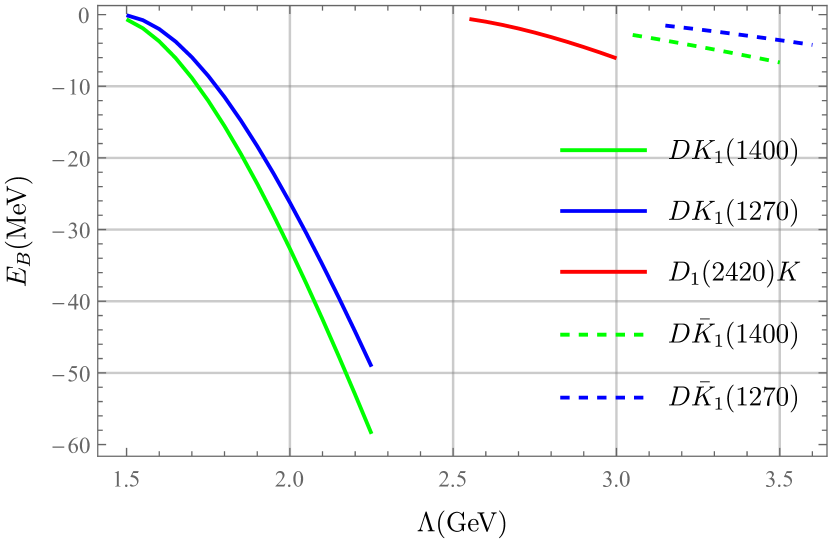
Figure 2: Binding energies v.s. cutoff $\Lambda$ for different isoscalar systems.

The interactions we considered above also work in the $DK$ system. The parameters that produce a $DK$ bound state corresponding to $D_{s0}(2317)$ can also result in a $D_{1}K$ bound state with a similar binding energy, but cannot bind $\bar{D}_{1}K$ together.

These calculation can be easily extended to the $B_{1}K$ and $BK_{1}$ cases. The interactions should be the same due to the heavy quark symmetry. For $B_{1}K$, the reduced mass is almost the same as that of $B_{1}K$ and hence a large cutoff $\Lambda\gtrsim 2.6$ GeV is needed to produce bound states. While for $BK_{1}$, the reduced mass gets larger than that of $DK_{1}$ and hence deeper bound states than $DK_{1}$ are expected. For example, the binding energy of $DK_{1}(1400)$ and $BK_{1}(1400)$ are $15$ and $50$ MeV when $\Lambda=1.8$ GeV.

III The decay properties of $DK_{1}$ molecules

Figure 3: Two-body and three-body decays of molecules composed of $DK_{1}$.

With reasonable cutoff we obtain the possible bound states of $DK_{1}(1400)$ and $DK_{1}(1270)$, denoted by $X$, whose binding energies lie in the range of $0\sim$ 30 MeV. It is now desirable to estimate the decay patterns of the predicted molecular states to provide some guidance of their experimental search. We assume that such molecules decay through their components as illustrated in Fig.3. Since $K_{1}$’s have quite large decay widths, we assume that the three-body decays of molecules are dominated by the one shown in Fig.3 where $P,V=\pi,K^{*}$ or $K,\rho/\omega$. All possible two-body strong decay channels are listed in Table 2. Note that some exchanged particles in this table are marked by underlines because these diagrams are expected to have much smaller contributions than others. Therefore, we do not consider these diagrams for simplicity.

Table 2: Two-body decay channels for the $DK_{1}$ molecule states considered in our calculation. Diagrams with heavier exchanged particles marked by underlines are much smaller and dropped in our calculation.

Final states	Exchanged particles
$D^{*}K^{*}$	$\pi$
$DK$, $D^{*}K$, $DK^{*}$ $D_{1}K$	$\rho$, $\omega$
$D_{s}^{*}\eta$, $D^{*}_{s}\eta^{\prime}$, $D_{s}\eta$, $D_{s}\eta^{\prime}$	$K^{*}$, $D^{*}$
$D_{s}^{*}\omega$	$K$, $K^{*}$, $D$, $D^{*}$
$D_{s}^{*}\phi$	$K$, $\underline{K^{*}}$

The coupling between a molecule and its components can be estimated model-independently via Weinberg compositeness criterion Weinberg (1965); Baru et al. (2004), namely,

$$\mathcal{L}_{XDK_{1}}=yX^{\mu}D^{\dagger}K^{\dagger}_{1\mu}+h.c.$$ (36)

with

$$y^{2}=16\pi(m_{D}+m_{K_{1}})^{5/2}\sqrt{\frac{2E_{b}}{m_{D}m_{K_{1}}}}.$$ (37)

In the following the binding energy will be fixed to $E_{b}=20$ MeV since Eq.(37) mainly contributes an overall factor to the total decay width and has little effect on the branching ratios of different channels.

To describe the transition from $DK_{1}$ to final states, the following Lagrangians, besides the ones introduced in the previous section, are needed.

$$\mathcal{L}_{APV} =ia\ {\rm Tr}(A_{\mu}[V^{\mu},P]),$$ (38)

$$\mathcal{L}_{BPV} =b\ {\rm{Tr}}(B_{\mu}\{V^{\mu},P\})$$ (39)

$$\mathcal{L}_{AVV} =a^{\prime}\epsilon^{\alpha\beta\gamma\delta}\left(\partial_{\alpha}K_{1,A\beta}^{+}\rho^{-}_{\gamma}\bar{K}^{*0}_{\delta}\right.$$

$$\left.+\partial_{\alpha}K_{1,A\beta}^{-}\rho^{+}_{\gamma}{K}^{*0}_{\delta}+\cdots\right)$$ (40)

$$\mathcal{L}_{BVV} =ib^{\prime}\epsilon^{\alpha\beta\gamma\delta}\left(\partial_{\alpha}K_{1,B\beta}^{+}\rho^{-}_{\gamma}\bar{K}^{*0}_{\delta}\right.$$

$$\left.-\partial_{\alpha}K_{1,B\beta}^{-}\rho^{+}_{\gamma}{K}^{*0}_{\delta}+\cdots\right)$$ (41)

$$\mathcal{L}_{{DD}^{*}{P}} =-\frac{2g}{f_{\pi}}\sqrt{{m}_{{D}}{m}_{{D}^{*}}}\left(D_{b}\left(\partial_{\mu}P_{ba}\right){D}_{a}^{*\mu\dagger}\right.$$

$$\left.-\overline{{D}}_{a}^{*\mu\dagger}\left(\partial_{\mu}P_{ab}\right)\overline{{D}}_{b}\right)$$ (42)

$$\mathcal{L}_{D^{*}{DV}} =i\sqrt{2}\lambda g_{V}\epsilon_{\alpha\beta\gamma\delta}\left((\partial^{\delta}D_{a})(\partial^{\alpha}V^{\beta}_{{ab}})D^{*\dagger\gamma}_{b}\right.$$

$$\left.-D_{a}(\partial^{\alpha}V^{\beta}_{{ab}})(\partial^{\delta}D^{*\dagger\gamma}_{b})\right)+h.c.$$ (43)

where the coupling constants are $g=0.3\sim 0.6$ Casalbuoni et al. (1997), $f_{\pi}=132$ MeV, $\lambda=0.6\ {\rm GeV}^{-1}$ Casalbuoni et al. (1993). In Ref. Divotgey et al. (2013) the coupling constants corresponding to the mixing angle $\phi=(56.4\pm 4.3)^{\circ}$ are estimated to be $a\approx 1.92\pm 0.09$ GeV and $b\approx-2.47\pm 0.08$ GeV. The coupling constants after mixing are listed in Tab.(3). Unlike $a$ and $b$ determined by partial decay widths of $K_{1}$, no direct experimental results are available for $a^{\prime}$ and $b^{\prime}$ and we use a quark model approach to estimate them as presented in the Appendix.

Table 3: Coupling constants of $K_{1}(1400)/K_{1}(1270)PV$.

	$K_{1}(1400)$	$K_{1}(1270)$
$K\rho$	$-a\sin(\phi)-b\cos(\phi)$	$a\cos(\phi)-b\sin(\phi)$
$K\omega$	$\sqrt{1/2}(-a\sin(\phi)-b\cos(\phi))$	$\sqrt{1/2}(a\cos(\phi)-b\sin(\phi))$
$K\phi$	$a\sin(\phi)-b\cos(\phi)$	$a\cos(\phi)+b\sin(\phi)$
$K^{*}\pi$	$a\sin(\phi)-b\cos(\phi)$	$a\cos(\phi)+b\sin(\phi)$
$K^{*}\eta_{8}$	$\sqrt{3/2}\,a\sin(\phi)+\sqrt{1/6}\,b\cos(\phi)$	$-\sqrt{3/2}\,a\cos(\phi)+\sqrt{1/6}\,b\sin(\phi)$
$K^{*}\eta_{0}$	$-\sqrt{4/3}\,b\cos(\phi)$	$-\sqrt{4/3}\,b\sin(\phi)$

When performing the loop integral in the triangle diagram of two-body decays, a Gaussian form factor

$$F_{0}(p,\Lambda_{0})=e^{-\bm{p}^{2}/\Lambda_{0}^{2}}$$ (44)

and a monopole form factor, Eq.(34), are introduced to the $XDK_{1}$ vertex and the propagator of the exchanged particle $A$, respectively. $\bm{p}$ is the three-momentum of the components in the rest frame of the molecule and $\Lambda_{0}$ plays the role of cutting high momentum components off in the wave function of the molecule.

Table 4: Partial decay width of the predicted $DK_{1}(1400)$ molecule. Here cutoffs are in unit of GeV while widths are in unity of MeV. $\alpha$E$\beta$ means $\alpha\times 10^{\beta}$. For the $DK^{*}$ channel, the sign of $a^{\prime}b^{\prime}$ is not determined and the results for both cases are listed here.

Final states	$\Lambda_{0}=0.6$			$\Lambda_{0}=1.0$
	$\Lambda=1.5$	$\Lambda=2.0$	$\Lambda=100$	$\Lambda=1.5$	$\Lambda=2.0$	$\Lambda=100$
$D^{*}K^{*}$	3.15	4.42	7.70	6.09	9.06	18.8
$D^{*}K$	7.1E-4	2.1E-3	0.010	1.9E-3	6.2E-3	0.035
$DK^{*}\ (a^{\prime}b^{\prime}>0)$	7.1E-3	0.012	0.11	0.020	0.068	0.48
$DK^{*}\ (a^{\prime}b^{\prime}<0)$	3.7E-6	6.0E-6	5.7E-5	1.0E-5	3.5E-5	2.5E-4
$DK$	1.4E-4	3.4E-4	7.8E-4	9.5E-4	2.2E-3	3.3E-3
$D_{s}\eta$	8.6E-4	2.2E-3	4.1E-3	6.3E-3	0.017	0.022
$D_{s}\eta^{\prime}$	9.7E-4	2.3E-3	3.7E-3	5.9E-3	0.015	0.019
$D_{s}^{*}\eta$	6.8E-3	0.025	0.12	0.018	0.069	0.44
$D_{s}^{*}\eta^{\prime}$	5.7E-3	0.020	0.096	0.014	0.055	0.33
$D_{1}K$	3.1E-3	6.0E-3	0.013	8.5E-3	0.018	0.048
$D_{s}^{*}\omega$	2.9E-3	4.9E-3	0.011	6.2E-3	0.011	0.030
$D_{s}^{*}\phi$	0.47	0.73	1.35	0.83	1.38	3.11
$DK\rho$	$0.049$
$DK\omega$	$0.015$
$DK^{*}\pi$	$27.0$
Total	31	32	36	34	38	50

Table 5: Partial decay width of the predicted $DK_{1}(1270)$ molecule. Same captions as Tab.(4)

Final states	$\Lambda_{0}=0.6$			$\Lambda_{0}=1.0$
	$\Lambda=1.5$	$\Lambda=2.0$	$\Lambda=100$	$\Lambda=1.5$	$\Lambda=2.0$	$\Lambda=100$
$D^{*}K^{*}$	0.63	0.81	1.22	1.00	1.37	2.38
$D^{*}K$	0.22	0.62	2.50	0.53	1.58	7.74
$DK^{*}\ (a^{\prime}b^{\prime}>0)$	1.5E-3	1.5E-3	0.024	2.6E-3	0.022	0.090
$DK^{*}\ (a^{\prime}b^{\prime}<0)$	9.0E-3	9.4E-3	0.016	0.015	0.13	0.54
$DK$	0.047	0.11	0.22	0.26	0.58	0.87
$D_{s}\eta$	3.4E-3	8.5E-3	0.014	0.021	0.055	0.072
$D_{s}\eta^{\prime}$	2.6E-3	5.7E-3	8.7E-3	0.013	0.031	0.040
$D_{s}^{*}\eta$	0.025	0.084	0.37	0.056	0.21	1.14
$D_{s}^{*}\eta^{\prime}$	3.3E-3	9.7E-3	0.033	6.6E-3	0.021	0.092
$D_{1}K$	0.96	1.72	3.43	2.25	4.39	10.9
$D_{s}^{*}\omega$	0.77	1.20	2.30	1.37	2.31	5.26
$DK\rho\to DK\pi\pi$	$4.56$
$DK^{*}\pi$	$3.32$
$D\pi K_{0}^{*}(1430)\to DK\pi\pi$	$5.69$
Total	16	18	24	19	24	42

The results for partial widths of the molecules are listed in Table 4 and Table 5. In our model, the absolute values of widths may suffer some uncertainty, resulting from the uncertainty of coupling constants as well as the choice of cutoffs. The former just mainly gives a scaling factor of order one to each channel. The latter one may also change the branching ratios of different channels but it turns out that the dominance of some decay channels is not influenced by the cutoffs. Due to the mixture nature of $K_{1}(1400)$ and $K_{1}(1270)$, the couplings of $K_{1}K\rho/\omega$ and $K_{1}K^{*}\pi$ are quite different. For the $DK_{1}(1400)$ molecule, three-body channel $DK^{*}\pi$ dominates and $D^{*}K^{*}$ channel also has considerable contribution due to the $\pi$ exchange. While for the $DK_{1}(1270)$ molecule, the partial decay widths to $D^{*}K$, $DK$, $D_{1}K$, $D_{s}^{*}\eta$ and $D_{s}^{*}\omega$ channels are not that small as the $K_{1}(1400)$ case because of the much larger coupling of $K_{1}(1270)K\rho/\omega$. Meanwhile the width of three-body channels become much smaller because of either small coupling of $K_{1}(1270)K\pi$ or vanishing phase space for $DK\rho/\omega$ and $DK_{0}^{*}(1430)\pi$. The finite width of $\rho$ or $K_{0}^{*}(1430)$ needs to be considered because $DK_{1}(1270)$ molecule lies below the threshold of $DK\rho$ or $DK_{0}^{*}(1430)\pi$ but $\rho$ and $K_{0}^{*}(1430)$ have quite large width. Here we consider the four body decay, $DK_{1}(1270)\to DK\rho(DK_{0}^{*}\pi)\to DK\pi\pi$ and refer to Ref. Jing et al. (2020) for elegant calculations of phase space integration.

IV Summary and Discussion

In this work we have calculate the potential between $DK_{1}$ or $D_{1}K$ systems to check if they are possible to form bound states. The interaction between these components are described by vector meson exchange model with effective Lagrangians. It turns out that for isoscalar systems, $DK_{1}$ or $D_{1}K$ are attractive but only in the former case is it possible to form bound states if the cutoff lies in the empirical region. Isovector systems have either repulsive or too weak attractive potentials and therefore, no bound states are expected. The $X_{1}(2900)$, recently reported by LHCb collaboration, makes it meaningful to explore the possibility of $\bar{D}_{1}K$ bound states since they can couple in S-wave and $X_{1}(2900)$ lies just about 10 MeV below $\bar{D}_{1}K$ threshold. Our results show that $\bar{D}_{1}K$ system, no matter isoscalar or isovector, can not be bound together via one meson exchange and the explanation of $X_{1}(2900)$ as a $\bar{D}_{1}K$ is disfavored.

The decay properties of the predicted isoscalar $DK_{1}$ molecules are calculated by applying Weinberg compositeness criterion. For the $DK_{1}(1400)$ bound state, due to the large width of $K_{1}(1400)\to K^{*}\pi$, the three-body channel $DK^{*}\pi$ dominates the total width of the bound states. Besides, $D^{*}K^{*}$ and $D_{s}^{*}\phi$ channels are also good places to search for the predicted molecule. While for the $DK_{1}(1270)$ bound state, it may be rewarding to look at the $D^{*}K^{*}$, $D^{*}K$, $D_{1}K$, $D_{s}^{*}\omega$ and $DK^{*}\pi$ channels.

The heavy quark symmetry allows one to predicted the corresponding bound states of $BK_{1}$ systems, whose binding energy are around $50$ MeV and the decay behaviors should be similar to those of $DK_{1}$ bound states.

Helpful discussions with Feng-Kun Guo, Hao-Jie Jing, Yong-Hui Lin and Mao-Jun Yan are acknowledged. This project is supported by NSFC under Grant No. 11621131001 (CRC110 cofunded by DFG and NSFC), Grant No. 11835015, No. 11947302, and by the Chinese Academy of Sciences (CAS) under Grants No. XDB34030303.

Appendix A Estimation of $g_{K_{1}K^{*}V}$

A.1 Effective Lagrangian on Hadron Level

The coupling of $K_{1}KV$ on hadron level can be constructed as

$$\mathcal{L}_{APV} =ia\operatorname{Tr}\left(A_{\mu}\left[V^{\mu},P\right]\right)=-iaK_{1,A\mu}^{+}\rho^{\mu-}\bar{K}^{0}+\cdots$$ (45)

$$\mathcal{L}_{BPV} =b\operatorname{Tr}\left(B_{\mu}\left\{V^{\mu},P\right\}\right)=bK_{1,B\mu}^{+}\rho^{\mu-}\bar{K}^{0}+\cdots$$ (46)

while for $K_{1}K^{*}V$,

$$\mathcal{L}_{AVV}= a^{\prime}\epsilon^{\alpha\beta\gamma\delta}\left(\partial_{\alpha}K_{1,A\beta}^{+}\rho^{-}_{\gamma}\bar{K}^{*0}_{\delta}\right.$$

$$\left.+\partial_{\alpha}K_{1,A\beta}^{-}\rho^{+}_{\gamma}{K}^{*0}_{\delta}+\cdots\right)$$ (47)

$$\mathcal{L}_{BVV}= ib^{\prime}\epsilon^{\alpha\beta\gamma\delta}\left(\partial_{\alpha}K_{1,B\beta}^{+}\rho^{-}_{\gamma}\bar{K}^{*0}_{\delta}\right.$$

$$\left.-\partial_{\alpha}K_{1,B\beta}^{-}\rho^{+}_{\gamma}{K}^{*0}_{\delta}+\cdots\right)..$$ (48)

We now aim at estimating $a^{\prime},b^{\prime}$ from $a,b$. Considering the mixing, Eq.(14), we have

$$g_{K_{1}(1270)K^{*}\rho}= (a^{\prime}\cos\varphi+b^{\prime}\sin(\varphi))$$ (49)

$$g_{K_{1}(1400)K^{*}\rho}= i(b^{\prime}\cos\varphi-a^{\prime}\sin(\varphi)).$$ (50)

In the nonrelativistic (NR) limit, the squared amplitudes after sum of polarizations read

$$\frac{1}{3}\sum|\mathcal{M}|^{2}\approx\left\{\begin{array}[]{ll}(a\ {\rm or\ }b)^{2}&\mathrm{for}\ K_{1}\to K\rho\\ (a^{\prime}\ {\rm or}\ b^{\prime})^{2}m_{K_{1}}^{2}&\mathrm{for}\ K_{1}\to K^{*}\rho\end{array}\right.$$ (53)

A.2 Effective Lagrangian from Quark Model

Analogous to the quark model describing $\gamma N$ interaction, see Ref. Close (1979) for a detailed discussion, the effective coupling of $K_{1}K^{(*)}V$ (essentially $qqV$ and we take $\rho$ meson as an example) can be constructed as

$$\mathcal{L}=g\left[2i\bm{s}^{j}\cdot(\bm{k}\times\bm{\rho})+2\bm{p}\cdot\bm{\rho}\right]$$ (54)

with $g$ the coupling constant, $\bm{s}$ the spin operator, $\bm{\rho}$ the vector field, $\bm{k}$ the 3-momentum of the vector and $\bm{q}$ the 3-momentum of the quark. This Lagrangian can be derived from the quark level. For a free fermion the Hamiltonian reads

$$H_{\rm{free}}=\frac{p^{2}}{2m}=\frac{\not{p}\not{p}}{2m}.$$ (55)

We introduced the coupling of a vector field to the quark by the following remedy,

$$H=\frac{(\not{p}-g\not{\rho})(\not{p}-g\not{\rho})}{2m}=H_{\rm{free}}+H_{\rm{int}}$$ (56)

where

$$H_{\rm{int}} \approx-g(\not{p}\not{\rho}+\not{\rho}\not{p})$$ (57)

with

$$\rho_{\mu}(x)=\int\frac{d^{3}k}{(2\pi)^{3}}\frac{1}{\sqrt{2E_{\bm{k}}}} \left(\epsilon_{\mu}(\bm{k})a_{\bm{k}}e^{-ip\cdot x}\right.$$

$$\left.+\left.\epsilon^{*}_{\mu}(\bm{k})a_{\mathbf{k}}^{\dagger}e^{ik\cdot x}\right)\right|_{k^{0}=E_{\mathbf{k}}}$$ (58)

After contracting with the external vector meson we have

$$H_{\rm{int}} \propto-g\frac{e^{ik\cdot x}}{\sqrt{2k^{0}}}(2p\cdot\epsilon^{*}+\not{k}\not{\epsilon}^{*}).$$ (59)

Considering the Dirac representation of $\gamma$ matrices

$$\gamma^{0} =\left(\begin{array}[]{cc}1&0\\ 0&-1\end{array}\right),$$ (62)

$$\gamma^{i} =\left(\begin{array}[]{cc}0&\sigma^{i}\\ -\sigma^{i}&0\end{array}\right),$$ (65)

$$\alpha^{i} =\gamma^{0}\gamma^{i}=\left(\begin{array}[]{cc}0&\sigma^{i}\\ \sigma^{i}&0\end{array}\right),$$ (68)

we obtain

$$H_{\rm{int}} \propto g\frac{e^{ik\cdot x}}{\sqrt{2k^{0}}}\left[2\bm{p}\cdot\bm{\epsilon}^{*}+i\bm{\sigma}\cdot(\bm{k}\times\bm{\epsilon}^{*})\right.$$

$$\left.-2(p^{0}\epsilon^{*0}+k^{0}\epsilon^{*0})+(k^{0}\bm{\epsilon}^{*}-\epsilon^{*0}\bm{k})\cdot\bm{\alpha}\right]$$ (69)

In the NR limit, $\epsilon^{0}=0$, $k^{0}=m_{\rho}$ and $\bm{\epsilon}^{*}\cdot\bm{\alpha}$ mix the large and small components of the spinor. After omitting these terms we obtain

$$H_{\rm{int}} \propto g\frac{e^{ik\cdot x}}{\sqrt{2m_{\rho}}}\left[2\bm{p}\cdot\bm{\epsilon}^{*}+i\bm{\sigma}\cdot(\bm{k}\times\bm{\epsilon}^{*})\right]$$

$$\propto e^{ik\cdot x}\left[2\bm{p}\cdot\bm{\epsilon}^{*}+i\bm{\sigma}\cdot(\bm{k}\times\bm{\epsilon}^{*})\right].$$ (70)

Note that the first term flips $L_{z}$ while the second one flips $S_{z}$.

The wave functions of related particles are collected in the following

$$|K_{1A}(1,m)\rangle= \sum_{m_{1}+m_{2}=m}\langle 1,m_{1},1,m_{2}|1,m\rangle\Psi_{1,m_{1}}\chi_{1,m_{2}}$$ (71)

$$|K_{1B}(1,m)\rangle= \Psi_{1,m}\chi_{0,0}$$ (72)

$$|\rho(1,m)\rangle= \chi_{1,m}$$ (73)

$$|K\rangle= \Psi_{0,0}\chi_{0,0}$$ (74)

$$|K^{*}(1,m)\rangle= \Psi_{0,0}\chi_{1,m}$$ (75)

where $\Psi$ and $\chi$ represent the spatial and spin wave functions, respectively. Then let’s fix the kinetics. $K_{1A/B}$ decays into $K^{(*)}\rho$ where $K_{1}$ is at rest with $P=(m_{K_{1}},0,0,0)$ and $\rho$ flies along the $z-$axis with $k=(m_{\rho},0,0,k)$. The polarization of $\rho$, represented by the $\bm{\epsilon}$ in the Lagrangian, reads explicitly

$$\bm{\epsilon}(1) =-\frac{1}{\sqrt{2}}(1,i,0)$$ (76)

$$\bm{\epsilon}(0) =(0,0,1)$$ (77)

$$\bm{\epsilon}(-1) =\frac{1}{\sqrt{2}}(1,-i,0)$$ (78)

and in turn

$$2\bm{p}\cdot\bm{\epsilon}^{*}+i\bm{\sigma}\cdot(\bm{k}\times\bm{\epsilon}^{*})=\left\{\begin{array}[]{ll}{\sqrt{2}}p_{-}-\frac{k}{\sqrt{2}}\sigma_{-}&\ {\rm for}\ \bm{\epsilon}(1)\\ 2p_{z}&\ {\rm for}\ \bm{\epsilon}(0)\\ {\sqrt{2}}p_{+}+\frac{k}{\sqrt{2}}\sigma_{+}&\ {\rm for}\ \bm{\epsilon}(-1)\\ \end{array}\right.$$ (82)

with $\sigma_{\pm}=\sigma_{x}\pm i\sigma_{y}$ and $p_{\pm}=p_{x}\pm ip_{y}$.

Now the calculation of the amplitude of $K_{1A/B}\to K^{(*)}\rho$ is straightforward. Let’s first define the following constants

$$l_{-}= \left|\langle\Psi_{0,0}|e^{-ikz}\sqrt{2}p_{-}|\Psi_{1,1}\rangle\right|^{2}$$ (83)

$$l_{+}= \left|\langle\Psi_{0,0}|e^{-ikz}\sqrt{2}p_{+}|\Psi_{1,-1}\rangle\right|^{2}$$ (84)

$$l_{0}= \left|\langle\Psi_{0,0}|e^{-ikz}2p_{z}|\Psi_{1,0}\rangle\right|^{2}$$ (85)

$$s_{0}= \left|\frac{k}{2\sqrt{2}}\langle\Psi_{0,0}|e^{-ikz}|\Psi_{1,0}\rangle\right|^{2}$$ (86)

and then we have

$$\frac{1}{3}\sum|\mathcal{M}|^{2}=\left\{\begin{array}[]{lll}\frac{2}{3}s_{0}&=a^{2}&\ {\rm for}\ K_{1A}\to K\rho\\ \frac{1}{3}(l_{+}+l_{-}+l_{0})&=b^{2}&\ {\rm for}\ K_{1B}\to K\rho\\ \frac{1}{3}\left(s_{0}+\frac{1}{2}(l_{+}+l_{-}+l_{0})\right)&=2a^{{}^{\prime}2}m_{K_{1A}}^{2}&\ {\rm for}\ K_{1A}\to K^{*}\rho\\ \frac{1}{3}s_{0}&=2b^{{}^{\prime}2}m_{K_{1B}}^{2}&\ {\rm for}\ K_{1B}\to K^{*}\rho\end{array}\right.$$ (91)

$a=1.92\ {\rm GeV}$, $b=-2.47\ {\rm GeV}$, $m_{K_{1A}}=1.36\ \mathrm{GeV}$ and $m_{K_{1B}}=1.31\ \mathrm{GeV}$ as inputs yield $|a^{\prime}|=1.15$ and $|b^{\prime}|=0.73$. The relative sign of $a^{\prime}$ and $b^{\prime}$ can not be determined within this model.

References

- Aaij et al. (2020) R. Aaij et al. (LHCb), Phys. Rev. D 102, 112003 (2020), arXiv:2009.00026 [hep-ex] .
- Karliner and Rosner (2020) M. Karliner and J. L. Rosner, Phys. Rev. D 102, 094016 (2020), arXiv:2008.05993 [hep-ph] .
- He et al. (2020) X.-G. He, W. Wang, and R. Zhu, Eur. Phys. J. C 80, 1026 (2020), arXiv:2008.07145 [hep-ph] .
- Zhang (2021) J.-R. Zhang, Phys. Rev. D 103, 054019 (2021), arXiv:2008.07295 [hep-ph] .
- Wang (2020) Z.-G. Wang, Int. J. Mod. Phys. A 35, 2050187 (2020), arXiv:2008.07833 [hep-ph] .
- Lü et al. (2020) Q.-F. Lü, D.-Y. Chen, and Y.-B. Dong, Phys. Rev. D 102, 074021 (2020), arXiv:2008.07340 [hep-ph] .
- Chen et al. (2020) H.-X. Chen, W. Chen, R.-R. Dong, and N. Su, Chin. Phys. Lett. 37, 101201 (2020), arXiv:2008.07516 [hep-ph] .
- Hu et al. (2021) M.-W. Hu, X.-Y. Lao, P. Ling, and Q. Wang, Chin. Phys. C 45, 021003 (2021), arXiv:2008.06894 [hep-ph] .
- Liu et al. (2020a) M.-Z. Liu, J.-J. Xie, and L.-S. Geng, Phys. Rev. D 102, 091502 (2020a), arXiv:2008.07389 [hep-ph] .
- He and Chen (2020) J. He and D.-Y. Chen, (2020), arXiv:2008.07782 [hep-ph] .
- Huang et al. (2020) Y. Huang, J.-X. Lu, J.-J. Xie, and L.-S. Geng, Eur. Phys. J. C 80, 973 (2020), arXiv:2008.07959 [hep-ph] .
- Xue et al. (2021) Y. Xue, X. Jin, H. Huang, and J. Ping, Phys. Rev. D 103, 054010 (2021), arXiv:2008.09516 [hep-ph] .
- Molina and Oset (2020) R. Molina and E. Oset, Phys. Lett. B 811, 135870 (2020), arXiv:2008.11171 [hep-ph] .
- Agaev et al. (2020) S. Agaev, K. Azizi, and H. Sundu, (2020), arXiv:2008.13027 [hep-ph] .
- Liu et al. (2020b) X.-H. Liu, M.-J. Yan, H.-W. Ke, G. Li, and J.-J. Xie, Eur. Phys. J. C 80, 1178 (2020b), arXiv:2008.07190 [hep-ph] .
- Burns and Swanson (2021a) T. J. Burns and E. S. Swanson, Phys. Lett. B 813, 136057 (2021a), arXiv:2008.12838 [hep-ph] .
- Albuquerque et al. (2021) R. M. Albuquerque, S. Narison, D. Rabetiarivony, and G. Randriamanatrika, Nucl. Phys. A 1007, 122113 (2021), arXiv:2008.13463 [hep-ph] .
- Chen et al. (2021) Y.-K. Chen, J.-J. Han, Q.-F. Lü, J.-P. Wang, and F.-S. Yu, J. Phys. G: Nucl. Part. Phys. 48 055007 81, 71 (2021), arXiv:2009.01182 [hep-ph] .
- Mutuk (2021) H. Mutuk, J. Phys. G: Nucl. Part. Phys. 48, 055007 (2021), arXiv:2009.02492 [hep-ph] .
- Burns and Swanson (2021b) T. J. Burns and E. S. Swanson, Phys. Rev. D 103, 014004 (2021b), arXiv:2009.05352 [hep-ph] .
- Wang et al. (2021) G.-J. Wang, L. Meng, L.-Y. Xiao, M. Oka, and S.-L. Zhu, Eur. Phys. J. C 81, 188 (2021), arXiv:2010.09395 [hep-ph] .
- Xiao et al. (2021) C.-J. Xiao, D.-Y. Chen, Y.-B. Dong, and G.-W. Meng, Phys. Rev. D 103, 034004 (2021), arXiv:2009.14538 [hep-ph] .
- Molina et al. (2010) R. Molina, T. Branz, and E. Oset, Phys. Rev. D 82, 014010 (2010), arXiv:1005.0335 [hep-ph] .
- Agaev et al. (2021) S. S. Agaev, K. Azizi, and H. Sundu, (2021), arXiv:2103.06151 [hep-ph] .
- Tan and Ping (2020) Y. Tan and J. Ping, (2020), arXiv:2010.04045 [hep-ph] .
- Qi et al. (2021) J.-J. Qi, Z.-Y. Wang, Z.-F. Zhang, and X.-H. Guo, (2021), arXiv:2101.06688 [hep-ph] .
- Choi et al. (2003) S. Choi et al. (Belle), Phys. Rev. Lett. 91, 262001 (2003), arXiv:hep-ex/0309032 .
- Guo et al. (2018) F.-K. Guo, C. Hanhart, U.-G. Meißner, Q. Wang, Q. Zhao, and B.-S. Zou, Rev. Mod. Phys. 90, 015004 (2018), arXiv:1705.00141 [hep-ph] .
- Dong et al. (2020) X.-K. Dong, Y.-H. Lin, and B.-S. Zou, Phys. Rev. D 101, 076003 (2020), arXiv:1910.14455 [hep-ph] .
- Dong et al. (2021) X.-K. Dong, F.-K. Guo, and B.-S. Zou, Progr. Phys. 41, 65 (2021), arXiv:2101.01021 [hep-ph] .
- Aubert et al. (2003) B. Aubert et al. (BaBar), Phys. Rev. Lett. 90, 242001 (2003), arXiv:hep-ex/0304021 .
- Besson et al. (2003) D. Besson et al. (CLEO), Phys. Rev. D 68, 032002 (2003), [Erratum: Phys.Rev.D 75, 119908 (2007)], arXiv:hep-ex/0305100 .
- Chen et al. (2017) H.-X. Chen, W. Chen, X. Liu, Y.-R. Liu, and S.-L. Zhu, Rept. Prog. Phys. 80, 076201 (2017), arXiv:1609.08928 [hep-ph] .
- Liu et al. (2013) L. Liu, K. Orginos, F.-K. Guo, C. Hanhart, and U.-G. Meissner, Phys. Rev. D 87, 014508 (2013), arXiv:1208.4535 [hep-lat] .
- Martínez Torres et al. (2015) A. Martínez Torres, E. Oset, S. Prelovsek, and A. Ramos, JHEP 05, 153 (2015), arXiv:1412.1706 [hep-lat] .
- Bali et al. (2017) G. S. Bali, S. Collins, A. Cox, and A. Schäfer, Phys. Rev. D 96, 074501 (2017), arXiv:1706.01247 [hep-lat] .
- Cheung et al. (2021) G. K. C. Cheung, C. E. Thomas, D. J. Wilson, G. Moir, M. Peardon, and S. M. Ryan (Hadron Spectrum), JHEP 02, 100 (2021), arXiv:2008.06432 [hep-lat] .
- Guo and Meissner (2011) F.-K. Guo and U.-G. Meissner, Phys. Rev. D 84, 014013 (2011), arXiv:1102.3536 [hep-ph] .
- Casalbuoni et al. (1997) R. Casalbuoni, A. Deandrea, N. Di Bartolomeo, R. Gatto, F. Feruglio, and G. Nardulli, Phys. Rept. 281, 145 (1997), arXiv:hep-ph/9605342 [hep-ph] .
- Ding (2009) G.-J. Ding, Phys. Rev. D 79, 014001 (2009), arXiv:0809.4818 [hep-ph] .
- Bando et al. (1988) M. Bando, T. Kugo, and K. Yamawaki, Phys. Rept. 164, 217 (1988).
- Isola et al. (2003) C. Isola, M. Ladisa, G. Nardulli, and P. Santorelli, Phys. Rev. D68, 114001 (2003), arXiv:hep-ph/0307367 [hep-ph] .
- Burakovsky and Goldman (1997) L. Burakovsky and J. T. Goldman, Phys. Rev. D56, R1368 (1997), arXiv:hep-ph/9703274 [hep-ph] .
- Suzuki (1993) M. Suzuki, Phys. Rev. D47, 1252 (1993).
- Cheng (2003) H.-Y. Cheng, Phys. Rev. D67, 094007 (2003), arXiv:hep-ph/0301198 [hep-ph] .
- Yang (2011) K.-C. Yang, Phys. Rev. D84, 034035 (2011), arXiv:1011.6113 [hep-ph] .
- Hatanaka and Yang (2008) H. Hatanaka and K.-C. Yang, Phys. Rev. D77, 094023 (2008), [Erratum: Phys. Rev.D78,059902(2008)], arXiv:0804.3198 [hep-ph] .
- Tayduganov et al. (2012) A. Tayduganov, E. Kou, and A. Le Yaouanc, Phys. Rev. D85, 074011 (2012), arXiv:1111.6307 [hep-ph] .
- Divotgey et al. (2013) F. Divotgey, L. Olbrich, and F. Giacosa, Eur. Phys. J. A49, 135 (2013), arXiv:1306.1193 [hep-ph] .
- Zhang et al. (2018) Z.-Q. Zhang, H. Guo, and S.-Y. Wang, Eur. Phys. J. C78, 219 (2018), arXiv:1705.00524 [hep-ph] .
- Roca et al. (2005) L. Roca, E. Oset, and J. Singh, Phys. Rev. D72, 014002 (2005), arXiv:hep-ph/0503273 [hep-ph] .
- Geng et al. (2007) L. S. Geng, E. Oset, L. Roca, and J. A. Oller, Phys. Rev. D75, 014017 (2007), arXiv:hep-ph/0610217 [hep-ph] .
- Wang et al. (2019) G. Y. Wang, L. Roca, and E. Oset, Phys. Rev. D100, 074018 (2019), arXiv:1907.09188 [hep-ph] .
- Zhang et al. (2006) Y.-J. Zhang, H.-C. Chiang, P.-N. Shen, and B.-S. Zou, Phys. Rev. D74, 014013 (2006), arXiv:hep-ph/0604271 [hep-ph] .
- Weinberg (1966) S. Weinberg, Phys. Rev. Lett. 17, 616 (1966).
- Tomozawa (1966) Y. Tomozawa, Nuovo Cim. A 46, 707 (1966).
- Wang et al. (2013) Q. Wang, C. Hanhart, and Q. Zhao, Phys. Rev. Lett. 111, 132003 (2013), arXiv:1303.6355 [hep-ph] .
- Chen et al. (2019) Y.-H. Chen, L.-Y. Dai, F.-K. Guo, and B. Kubis, Phys. Rev. D 99, 074016 (2019), arXiv:1902.10957 [hep-ph] .
- Tornqvist (1994) N. A. Tornqvist, Z. Phys. C61, 525 (1994), arXiv:hep-ph/9310247 [hep-ph] .
- Weinberg (1965) S. Weinberg, Phys. Rev. 137, B672 (1965).
- Baru et al. (2004) V. Baru, J. Haidenbauer, C. Hanhart, Y. Kalashnikova, and A. E. Kudryavtsev, Phys. Lett. B 586, 53 (2004), arXiv:hep-ph/0308129 .
- Casalbuoni et al. (1993) R. Casalbuoni, A. Deandrea, N. Di Bartolomeo, R. Gatto, F. Feruglio, and G. Nardulli, Phys. Lett. B 299, 139 (1993), arXiv:hep-ph/9211248 .
- Jing et al. (2020) H.-J. Jing, C.-W. Shen, and F.-K. Guo, (2020), arXiv:2005.01942 [hep-ph] .
- Close (1979) F. E. Close, An introduction to quarks and partons (Academic Press, 1979).