Robust Finite-State Controllers for Uncertain POMDPs

Abstract

Uncertain partially observable Markov decision processes (uPOMDPs) allow the probabilistic transition and observation functions of standard POMDPs to belong to a so-called uncertainty set. Such uncertainty, referred to as epistemic uncertainty, captures uncountable sets of probability distributions caused by, for instance, a lack of data available. We develop an algorithm to compute finite-memory policies for uPOMDPs that robustly satisfy specifications against any admissible distribution. In general, computing such policies is theoretically and practically intractable. We provide an efficient solution to this problem in four steps. (1) We state the underlying problem as a nonconvex optimization problem with infinitely many constraints. (2) A dedicated dualization scheme yields a dual problem that is still nonconvex but has finitely many constraints. (3) We linearize this dual problem and (4) solve the resulting finite linear program to obtain locally optimal solutions to the original problem. The resulting problem formulation is exponentially smaller than those resulting from existing methods. We demonstrate the applicability of our algorithm using large instances of an aircraft collision-avoidance scenario and a novel spacecraft motion planning case study.

1 Introduction

In sequential decision making, one has to account for various sources of uncertainty. Examples for such sources are lossy long-range communication channels with a spacecraft orbiting the earth, or the expected responses of a human operator in a decision support system (Kochenderfer 2015). Moreover, sensor limitations may lead to imperfect information of the current state of the system. The standard models to reason about decision-making under uncertainty and imperfect information are partially observable Markov decision processes (POMDPs) (Kaelbling, Littman, and Cassandra 1998).

The likelihood of uncertain events, like a message loss in communication channels or of specific responses by human operators, is often only estimated from data. Yet, such likelihoods enter a POMDP model as concrete probabilities. POMDPs, in fact, require precise transition and observation probabilities. Uncertain POMDPs (uPOMDPs) remove this assumption by incorporating uncertainty sets of probabilities (Burns and Brock 2007). These sets are part of the transition and observation model in uPOMDPs and take the form of, for example, probability intervals or likelihood functions (Givan, Leach, and Dean 2000; Nilim and Ghaoui 2005). Such uncertainty is commonly called epistemic, which is induced by a lack of precise knowledge as opposed to aleatoric uncertainty, which is due to stochasticity.

Motivating example.

Consider a robust spacecraft motion planning system which serves as decision support for a human operator. This system delivers advice on switching to a different orbit or avoiding close encounters with other objects in space. Existing POMDP models assume that a fixed probability captures the responsiveness of the human (Kochenderfer 2015). However, a single probability may not faithfully capture the responsiveness of multiple operators. Instead of using a single probability, we use bounds on the actual value of this probability and obtain a uPOMDP model.

A policy for the decision support system necessarily considers all potential probability distributions and may need to predict the current location of the spacecraft based on its past trajectory. Therefore, it requires robustness against the uncertainty, and memory to store past (observation) data.

Problem formulation.

The general problem we address is: For a uPOMDP, compute a policy that is robust against all possible probabilities from the uncertainty set. Even without uncertainties, the problem is undecidable (Madani, Hanks, and Condon 1999). Most research has focused on either belief-based approaches or on computing finite state controllers (FSCs) (Meuleau et al. 1999; Amato, Bernstein, and Zilberstein 2010). Our approach extends the latter and computes robust FSCs representing robust policies.

Contribution and Approach

We develop a novel solution for efficiently computing robust policies for uPOMDPs using robust convex optimization techniques. The method solves uPOMDPs with hundreds of thousands of states, which is out of reach for the state-of-the-art.

Finite memory.

The first step of our method is to obtain a tractable representation of memory. As a concise representation of uPOMDP policies with finite memory, we utilize FSCs. First, we build the product of the FSC memory and the uPOMDP. Computing a policy with finite memory for the original uPOMDP is equivalent to computing a memoryless policy on the product (Junges et al. 2018). While the problem complexity remains NP-hard (Vlassis, Littman, and Barber 2012), the problem size grows polynomially in the size of the FSC. Existing methods cannot cope with that blow-up, as our experiments demonstrate.

Semi-infinite problem.

We state the uPOMDP problem as a semi-infinite nonconvex optimization problem with infinitely many constraints. A tailored dualization scheme translates this problem into a finite optimization problem with a linear increase in the number of variables. Combining this dualization with a linear-time transformation of the uPOMDP to a so-called simple uPOMDP (Junges et al. 2018) ensures exact solutions to the original problem. The exact solutions and the moderate increase in the problem size contrasts with an over-approximative solution computed using an exponentially larger encoding proposed in (Suilen et al. 2020).

Finite nonconvex problem.

The resulting finite optimization problem is still nonconvex and infeasible to solve exactly (Alizadeh and Goldfarb 2003; Lobo et al. 1998). We adapt a sequential convex programming (SCP) scheme (Mao et al. 2018) that iteratively linearizes the problem around previous solutions. Three extensions help to alleviate the errors introduced by the linearization, rendering the method sound for the uPOMDP problem.

Numerical experiments.

We demonstrate the applicability of the approach using two case studies. Notably, we introduce a novel robust spacecraft motion planning scenario. We show that our method scales to significantly larger models than (Suilen et al. 2020). This scalability advantage allows more precise models and adding memory to the policies.

Related work

Uncertain MDPs with full observability have been extensively studied, see for instance (Wolff, Topcu, and Murray 2012; Puggelli et al. 2013; Hahn et al. 2017). For uPOMDPs, (Suilen et al. 2020) is also based on convex optimization. However, their resulting optimization problems are exponentially larger than ours, and they only consider memoryless policies. (Burns and Brock 2007) utilizes sampling-based methods and (Osogami 2015) employs a robust value iteration on the belief space of the uPOMDP. (Ahmadi et al. 2018) uses sum-of-squares optimization to verify uPOMDPs against temporal logic specifications. The work in (Itoh and Nakamura 2007) assume distributions over the probability values of the uncertainty set. Finally, (Chamie and Mostafa 2018) considers a convexified belief space and computes a policy that is robust over this space.

2 Background and Formal Problem

Uncertain POMDPs.

The set of all probability distributions over a finite or countably infinite set $X$ is $\mathit{Distr}(X)$.

Definition 1 (uPOMDP).

An uncertain partially observable Markov decision process (uPOMDP) is a tuple $\mathcal{M}{}=(S{},s_{\mathit{I}}{},\mathit{A},\mathbb{I},\mathcal{P}{},{Z}{},{O}{},R)$ with a finite set $S$ of states, an initial state $s_{\mathit{I}}\in S$, a finite set $\mathit{A}$ of actions, a set $\mathbb{I}$ of probability intervals, an uncertain transition function $\mathcal{P}\colon S\times\mathit{A}\times S\to\mathbb{I}$, a finite set ${Z}$ of observations, an uncertain observation function ${O}\colon S\times{Z}\to\mathbb{I}$, and a reward function $R\colon S\times\mathit{A}\to\mathbb{R}_{\geq 0}$.

Nominal probabilities are point intervals where the upper and lower bounds coincide. If all probabilities are nominal, the model is a (nominal) POMDP. We see uPOMDPs as sets of nominal POMDPs that vary only in their transition function. For a transition function $P\colon S\times\mathit{A}\times S\to\mathbb{R}$, we write $P\in\mathcal{P}$ if for all $s,s^{\prime}\in S$ and $\alpha\in\mathit{A}$ we have $P(s,\alpha,s^{\prime})\in\mathcal{P}(s,\alpha,s^{\prime})$ and $P(s,\alpha,\cdot)$ is a probability distribution over $S$. Finally, a fully observable uPOMDP where each state has unique observations is an uncertain MDP.

Policies.

An observation-based policy $\mathit{\sigma}\colon(Z\times\mathit{A})^{*}\times Z\rightarrow\mathit{Distr}(\mathit{A})$ for a uPOMDP maps a trace, i.e., a sequence of observations and actions, to a distribution over actions. A finite-state controller (FSC) consists of a finite set of memory states and two functions. The action mapping $\gamma(n,z)$ takes an FSC memory state $n$ and an observation $z$, and returns a distribution over uPOMDP actions. To change a memory state, the memory update $\eta(n,z,\alpha)$ returns a distribution over memory states and depends on the action $\alpha$ selected by $\gamma$. An FSC induces an observation-based policy by following a joint execution of these functions upon a trace of the uPOMDP. An FSC is memoryless if there is a single memory state. Such FSCs encode policies $\mathit{\sigma}\colon Z\rightarrow\mathit{Distr}(\mathit{A})$.

Specifications.

We constrain the undiscounted expected reward (the value) of a policy for a uPOMDP using specifications: For a POMDP $\mathcal{M}$ and a set of goal states $G$ the specification $\mathbb{E}_{\geq\kappa}(\lozenge G)$ states that the expected reward before reaching $G$ is at least $\kappa$. For brevity, we require that the POMDP has no dead-ends, i.e., that under every policy, we eventually reach $G$. Reachability specifications to a subset of $G$ and discounted rewards are special cases (Puterman 1994).

Satisfying specifications.

A policy $\mathit{\sigma}$ satisfies a specification $\varphi=\mathbb{E}_{\geq\kappa}(\lozenge G)$, if the expected reward to reach $G$ induced by $\mathit{\sigma}$ is at least $\kappa$. POMDP $\mathcal{M}[P]$ denotes the instantiated uPOMDP $\mathcal{M}$ with a fixed transition function $P\in\mathcal{P}$. A policy robustly satisfies $\varphi$ for the uPOMDP $\mathcal{M}$, if it does so for all $\mathcal{M}[P]$ with $P\in\mathcal{P}$. Thus, a (robust) policy for uPOMDPs accounts for all possible instantiations $P\in\mathcal{P}$.

Formal problem statement.

Given a uPOMDP $\mathcal{M}$ and a specification $\varphi$, compute an FSC that yields an observation-based policy $\mathit{\sigma}$ which robustly satisfies $\varphi$ for $\mathcal{M}$.

Assumptions.

We compute the product of the memory update of an FSC and the uPOMDP and reduce the problem do computing policies without memory (Junges et al. 2018). Therefore, we focus in the following on memoryless policies and show the impact of finite memory in our examples.

For the correctness of our method, instantiations are not allowed to remove transitions. That is, for any interval we either require the lower bound to be strictly greater than $0$ such that the transition exists in all instantiations, or both upper and lower bound to be equal to $0$ such that the transition does not exist in all instantiations. This assumption is standard and for instance used in (Wiesemann, Kuhn, and Rustem 2013).

Outline.

In Sect. 3, we equivalently formulate our problem as semi-infinite nonlinear problem (NLP). In Sect. 4, we translate this semi-infinite NLP can be transformed into a finite NLP. Then, in Sect. 5, we linearize the finite NLP into a finite linear program, and solve the resulting linear program (LP), inspired by so-called sequential convex programming methods. In Sect. 6, we evaluate our method.

3 Optimization Problem for uPOMDPs

In this section, we reformulate our problem statement as a semi-infinite nonconvex optimization problem, with finitely many variables but infinitely many constraints. We utilize simple uPOMDPs, defined below, as the dualization discussed in Sect. 4 is exact (only) for simple uPOMDPs.

We adopt a small extension of (PO)MDPs in which only a subset of the actions are available in a state, i.e., the transition function should be interpreted as a partial function. We denote the set of actions at state $s$ by $\mathit{A}(s)$. We ensure that states sharing an observation share the set of available actions. Moreover, we translate the observation function to be deterministic without uncertainty, i.e., of the form ${O}\colon S\rightarrow{Z}$, by expanding the state space (Chatterjee et al. 2016).

Definition 2 (Binary/Simple uPOMDP).

A uPOMDP is binary, if $|\mathit{A}(s)|\leq 2$ for all $s\in S.$ A binary uPOMDP is simple if for all $s\in S$, the following is true:

$$|\mathit{A}(s)|=2\;\text{implies}\;\forall\alpha\in\mathit{A}(s),\;\exists s^{\prime}\in S,\;\mathcal{P}(s,\alpha,s^{\prime})=1,$$

Simple uPOMDPs differentiate the states with action choices and uncertain outcomes. All uPOMDPs can be transformed into simple uPOMDPs. We refer to (Junges et al. 2018) for a transformation. This transformation preserves the optimal expected reward of a uPOMDP.

Let $S_{\mathrm{a}}$ denote the states with action choices, and $S_{\mathrm{u}}$ denote the states with uncertain outcomes. We now introduce the optimization problem with the nonnegative reward variables $\{r_{s}\geq 0\;|\;s\in S\}$ denoting the expected reward before reaching goal set $G$ from state s, and positive variables $\{\sigma_{s,\alpha}>0\;|\;s\in S,\alpha\in\mathit{A}(s)\}$ denoting the probability of taking an action $\alpha$ in a state $s$ for the policy. Note that we only consider policies where for all states $s$ and actions $\alpha$ it holds that $\sigma_{s,\alpha}>0$, such that applying the policy to the uPOMDP does not change the underlying graph.

$$\begin{aligned} \text{maximize}\quad&r_{s_{I}}\end{aligned}$$ (1)

$$\begin{aligned} \text{subject to}\quad\,\,r_{s_{I}}\geq\kappa,\quad\forall s\in G,\quad&r_{s}=0,\end{aligned}$$ (2)

$$\begin{aligned} \forall s\in S,\quad&\sum\nolimits_{\alpha\in\mathit{A}(s)}\sigma_{s,\alpha}=1,\end{aligned}$$ (3)

$$\begin{aligned} \forall s,s^{\prime}\in S\text{ s.t.\ }{O}(s)={O}(s^{\prime}),\forall\alpha\in\mathit{A}(s),\;\sigma_{s,\alpha}=\sigma_{s^{\prime},\alpha},\end{aligned}$$ (4)

$$\begin{aligned} &\!\forall s\in S_{\mathrm{a}},\,r_{s}\leq\!\!\!\sum_{\alpha\in\mathit{A}(s)}\!\!\!\sigma_{s,\alpha}\!\cdot\!\scalerel*[5pt]{\big{(}}{\ensurestackMath{\addstackgap[1.5pt]{\big{(}}}}R(s,\alpha)\!+\!\!\sum_{s^{\prime}\in S}\!\mathcal{P}(s,\alpha,s^{\prime})\cdot r_{s^{\prime}}\scalerel*[5pt]{\big{)}}{\ensurestackMath{\addstackgap[1.5pt]{\big{)}}}},\end{aligned}$$ (5)

$$\begin{aligned} &\forall s\in S_{\mathrm{u}},\,\forall P\in\mathcal{P},\;\,r_{s}\leq R(s)+\sum_{s^{\prime}\in S}P(s,s^{\prime})\cdot r_{s^{\prime}}.\end{aligned}$$ (6)

The objective is to maximize the expected reward $r_{s_{I}}$ at the initial state. The constraint (2) encodes the specification requirement and assigns the expected reward to $0$ in the states of goal set $G$. We ensure that the policy is a valid probability distribution in each state by (3). Next, (4) ensures that the policy is observation-based. We encode the computation of expected rewards for states with action choices by (5) and with uncertain outcomes by (6). We omit denoting the unique actions in the transition function $P(s,s^{\prime})$ and reward function $R(s)$ in (6) for states with uncertain outcomes.

Let us consider some properties of the optimization problem. First, the functions in (5) are quadratic. Essentially, the policy variables $\sigma_{s,\alpha}$ are multiplied with the reward variables $r_{s}$. In general, these constraints are nonconvex, and we later linearize them. Second, the values of the transition probabilities $P(s,s^{\prime})$ for $s,s^{\prime}\in S_{\textrm{u}}$ in (6) belong to continuous intervals. Therefore, there are infinitely many constraints over a finite set of reward variables. These constraints are similar to the LP formulation for MDPs (Puterman 1994), and are affine; there are no policy variables.

4 Dualization of Semi-Infinite Constraints

In this section, we transform the semi-infinite optimization problem into a finite optimization problem using dualization for simple uPOMDPs. Specifically, we translate the semi-infinite constraints from (6) into finitely many constraints.

Dualization for Robust Linear Programs

We summarize robust LPs with polytopic uncertainty (Bertsimas, Brown, and Caramanis 2011; Ben-Tal, El Ghaoui, and Nemirovski 2009). The idea for solving robust LPs with such uncertainty is essential in our approach.

Robust LPs.

A robust LP with the variable $x\in\mathbb{R}^{n}$ is

$$\text{minimize}\quad c^{\top}x$$

$$\text{subject to}\quad(d+u)^{\top}x\leq e\quad\forall u\in\mathcal{U},$$

where $c,d\in\mathbb{R}^{n}$, and $e\in\mathbb{R}$ are given vectors, $u\in\mathbb{R}^{n}$ is the uncertain parameter, and $\mathcal{U}$ is the uncertainty set. We assume that the set $\mathcal{U}$ is a convex polytope, i.e., that it is an $n$-dimensional shape defined by the linear inequalities $Cu+g\geq 0$ for $C\in\mathbb{R}^{m\times n}$ and $g\in\mathbb{R}^{m}$.

Duality.

For simplicity, we explain the idea on a single robust inequality. The idea can be generalized to multiple robust inequalities. With $\mathcal{U}$ defined by the linear inequalities above, duality can be used to obtain a tractable solution to the robust LP. Specifically, we write the Lagrangian for the maximization problem over $u^{\top}x$ with the dual variable $\mu\geq 0$ as

$$L(u,\mu)=u^{\top}x+\mu^{\top}(Cu+g).$$

By taking the supremum over $u$, we obtain

$$\underset{u\in\mathcal{U}}{\text{sup}}\;\;L(u,\mu)=\begin{cases}\infty&\text{if }C^{\top}\mu+x\neq 0,\\ \mu^{\top}g&\text{if }C^{\top}\mu+x=0.\end{cases}$$

All inequalities are linear which implies strong duality, i.e.,

$$\underset{u\in\mathcal{U}}{\text{sup}}\;\;u^{\top}x=\underset{\mu\geq 0}{\text{inf}}\;\;\{\mu^{\top}g\;|\;C^{\top}\mu+x=0\}.$$

Since these optimization problems are linear, we know that the optimal value is attained at a feasible solution. Therefore, we can replace sup and inf with max and min. The semi-infinite inequality with polytopic uncertainty is equivalent to the following linear constraints

$$d^{\top}x+\mu^{\top}g\leq e,\quad C^{\top}\mu+x=0,\quad\mu\geq 0.$$

Dualization for Simple POMDPs

We now describe the dualization step that we use to obtain a finite optimization problem for simple POMDPs.

Uncertainty polytopes.

First, we formalize the uncertainty sets for simple uPOMDPs. For state $s\in S_{\mathrm{u}}$, we assume that there are $|S|$ intervals $[a_{s},b_{s}]\in\mathbb{I}$, $s\in S$ that describe the uncertain probability of transitioning to a successor state of $s$. This setting is equivalent to (Suilen et al. 2020).

The following constraints ensure that the uncertain transition function $P$ is well-defined at a state $s$:

$$\forall s^{\prime}\in S,\quad a_{s,s^{\prime}}\leq u_{s,s^{\prime}}\leq b_{s,s^{\prime}},\,\,\,\,\sum\nolimits_{s^{\prime}\in S}u_{s,s^{\prime}}=1.$$

We denote these constraints in matrix form: $C_{s}u+g_{s}\geq 0$.

Dualization.

After obtaining the matrices $C_{s}$ and vectors $g_{s}$ characterizing uncertainty sets for each state, we directly use dualization to transform the inequalities in (6) into

$$\forall s\in S_{\mathrm{u}},\,r_{s}\leq R(s)+\mu^{\top}_{s}g_{s},\,C^{\top}_{s}\mu_{s}+q=0,\,\mu_{s}\geq 0,$$ (7)

where $\mu_{s}\in\mathbb{R}^{|S|}$ is the dual variable of the constraint $C_{s}u+g_{s}\geq 0$ and $q$ is an $|S|-$dimensional vector denoting the set of reward variables for each state $s\in S$. After this step, the problem with the objective (1) and the constraints (2)–(5) and (7) has finitely many variables and constraints.

In the worst-case, the number of dual variables in (7) is $|S|\cdot|S_{u}|$, and the number of constraints is $2\cdot|S|\cdot|S_{u}|+|S_{u}|$, which only yields a factor $|S|$ of increase in the number of variables compared to the aforementioned semi-infinite optimization problem. In practice, most of the values of $a_{s,s^{\prime}}$, and $b_{s,s^{\prime}}$ are $0$, meaning there are few successor states for each state $s$, and we exploit this structure in our numerical examples.

5 Linearizing the Finite Nonconvex Problem

In this section, we discuss our algorithm to solve the (finite but nonconvex) dual problem from the previous section. Our method is based on a sequential convex programming (SCP) method (Yuan 2015; Mao et al. 2018). SCP iteratively computes a locally optimal solution to the dual problem from Section 4 by approximating it as an LP. In every iteration, this approximation is obtained by linearizing the quadratic functions around a previous solution. The resulting LP does not necessarily have a feasible solution, and the optimal solution does not necessarily correspond to a feasible solution of the original dual problem. We alleviate this drawback by adding three components to our approach.

Linearizing.

To linearize the dual problem, we only need to linearize the quadratic functions in (5), repeated below.

$$\!\forall s\in S_{\mathrm{a}},r_{s}\leq\!\!\sum_{\alpha\in\mathit{A}(s)}\!\!\!\sigma_{s,\alpha}\!\cdot\!\Big{(}R(s,\alpha)\!+\!\sum_{s^{\prime}\in S}\!\mathcal{P}(s,\alpha,s^{\prime})\cdot r_{s^{\prime}}\Big{)}$$

The constraint is quadratic in $r_{s}$ and $\sigma_{s,\alpha}$. For compact notation, let $h(s,\alpha,s^{\prime})$ be the quadratic function above for a given $s\in S_{\textrm{a}},s^{\prime}\in S$ and $\alpha\in\mathit{A}(s)$:

$$h(s,\alpha,s^{\prime})=\sigma_{s,\alpha}\cdot\mathcal{P}(s,\alpha,s^{\prime})\cdot r_{s^{\prime}}$$

and let $d=\mathcal{P}(s,\alpha,s^{\prime}),y=\sigma_{s,\alpha},\text{ and }z=r_{s^{\prime}}$. Let $\langle\hat{y},\hat{z}\rangle$ denote an arbitrary assignment to $y$ and $z$. We linearize $h(s,\alpha,s^{\prime})$ around $\langle\hat{y},\hat{z}\rangle$ as

$$h_{\textrm{aff}}(s,\alpha,s^{\prime}) =d\cdot\big{(}\hat{y}\cdot\hat{z}+\hat{y}\cdot(z-\hat{z})+\hat{z}\cdot(y-\hat{y})\big{)}$$

$$=d\cdot(\hat{y}\cdot z+\hat{z}\cdot y-\hat{z}\cdot\hat{y}).$$

The resulting function $h_{\textrm{aff}}(s,\alpha,s^{\prime})$ is affine in $y$ and $z$ ($r_{s}$ and $\sigma_{s,\alpha}$). After the linearization step, we replace (5) by

$$\!\forall s\in S_{\mathrm{a}},r_{s}\leq\!\!\!\sum_{\alpha\in\mathit{A}(s)}\!\!\!\sigma_{s,\alpha}\cdot\Big{(}R(s,\alpha)\!+\sum_{s^{\prime}\in S}h_{\textrm{aff}}(s,\alpha,s^{\prime})\Big{)}$$ (8)

Recall that the linearized problem may be infeasible, or the optimal solution to the linearized may no longer be feasible to the dual problem. We alleviate this issue as follows. First, we add penalty variables to the linearized constraints to ensure that the dual problem is always feasible, and we penalize violations by adding these variables to the objective. Second, we include trust regions around the previous solution to ensure that we do not deviate too much from this solution. Finally, we incorporate a robust verification step to ensure that the obtained policy satisfies the specification. This verification step is exact and alleviates the potential approximation errors that may arise in the linearization.

Penalty variables.

We add a nonnegative penalty variable $k_{s}$ for all $S_{\mathrm{a}}$ to the constraints in (8), which yields:

$$\forall s\in S_{\mathrm{a}},r_{s}\leq k_{s}+\!\!\!\sum_{\alpha\in\mathit{A}(s)}\!\!\!\sigma_{s,\alpha}\!\cdot\!\Big{(}R(s,\alpha)\!+\!\!\sum_{s^{\prime}\in S}h_{\textrm{aff}}(s,\alpha,s^{\prime})\Big{)}$$ (9)

When $k_{s}$ is sufficiently large, these constraints always allow a feasible solution. We also add a penalty variable to $r_{s_{I}}\geq\kappa$.

Trust regions.

We use trust regions by adding the following set of constraints to the resulting linearized problem:

$$\forall s\in S,\quad\nicefrac{{\hat{r}_{s}}}{{\delta^{\prime}}}\leq r_{s}\leq\hat{r}_{s}\cdot\delta^{\prime},$$ (10)

$$\forall s\in S_{\mathrm{a}},\;\forall\alpha\in\mathit{A}(s),\quad\nicefrac{{\hat{\sigma}_{s,\alpha}}}{{\delta^{\prime}}}\leq\sigma_{s,\alpha}\leq\hat{\sigma}_{s,\alpha}\cdot\delta^{\prime},$$ (11)

where $\delta^{\prime}=\delta+1$ and $\delta>0$ is the size of the trust region, which restricts the set of feasible policies, and $\hat{r}_{s}$ and $\hat{\sigma}_{s,\alpha}$ denotes the value of the reward and policy variables that are used for linearization.

Extended LP.

Combining these steps, we now state the resulting finite LP—for some fixed but arbitrary assignment to $\hat{r}_{s}$ and $\hat{\sigma}_{s,\alpha}$ in the definition of $h_{\textrm{aff}}$, penalty parameter $\tau>0$ and a trust region $\delta>0$:

$$\begin{aligned} \text{maximize}\quad&r_{s_{I}}-\tau\sum\nolimits_{s\in S_{\textrm{n}}}k_{s}\end{aligned}$$ (12)

$$\begin{aligned} \text{subject to}\quad\,\,r_{s_{I}}+k_{s_{I}}\geq\kappa,\;\;\forall s\in G,\quad&r_{s}=0,\end{aligned}$$ (13)

$$\begin{aligned} \forall s\in S,\quad&\sum\nolimits_{\alpha\in\mathit{A}(s)}\sigma_{s,\alpha}=1,\end{aligned}$$ (14)

$$\begin{aligned} \forall s,s^{\prime}\in S\text{ s.t.\ }{O}(s)={O}(s^{\prime}),\forall\alpha\in\mathit{A}(s),\;\sigma_{s,\alpha}=\sigma_{s^{\prime},\alpha},\end{aligned}$$ (15)

$$\begin{aligned} &\forall s\in S_{\mathrm{a}},r_{s}\leq k_{s}+\!\!\!\sum_{\alpha\in\mathit{A}(s)}\!\!\!\sigma_{s,\alpha}\!\cdot\!\Big{(}R(s,\alpha)\!+\!\!\sum_{s^{\prime}\in S}h_{\textrm{aff}}(s,\alpha,s^{\prime})\Big{)},\end{aligned}$$ (16)

$$\begin{aligned} &\forall s\in S_{\mathrm{u}},\,r_{s}\leq R(s)+\mu^{\top}_{s}g_{s},\;C^{\top}_{s}\mu_{s}+q=0,\;\mu_{s}\geq 0,\end{aligned}$$ (17)

$$\begin{aligned} \forall s\in S,\quad\nicefrac{{\hat{r}_{s}}}{{\delta^{\prime}}}\leq r_{s}\leq\hat{r}_{s}\cdot\delta^{\prime},\end{aligned}$$ (18)

$$\begin{aligned} \forall s\in S_{\mathrm{a}},\;\forall\alpha\in\mathit{A}(s),\quad\nicefrac{{\hat{\sigma}_{s,\alpha}}}{{\delta^{\prime}}}\leq\sigma_{s,\alpha}\leq\hat{\sigma}_{s,\alpha}\cdot\delta^{\prime}.\end{aligned}$$ (19)

1:Input: uPOMDP, specification with $\kappa$, $\gamma>1$, $\omega>0$

2:Initialize: trust region $\delta$, weight $\tau$, policy $\sigma$, $\beta_{\text{old}}=0$.

3:while $\delta>\omega$ do

4:   Verify the uncertain MC with policy $\sigma$:$\triangleright$ Step 1

5:   Extract reward variables ${r}_{s}$, objective value $\beta$.

6:   if $\lambda<\beta$ then $\triangleright$ Step 2

7:      return the policy $\sigma$ $\triangleright$ Found solution

8:   else if $\beta>\beta_{\text{old}}$ then

9:      $\forall s:\hat{r}_{s}\leftarrow r_{s}$, $\hat{\sigma}\leftarrow\sigma$, $\beta_{\text{old}}\leftarrow\beta$$\triangleright$ Accept iteration

10:      $\delta\leftarrow\delta\cdot\gamma$ $\triangleright$ Extend trust region

11:   else

12:      $\delta\leftarrow\delta/\gamma$ $\triangleright$ Reject iteration, reduce trust region

13:   end if

14:   Linearize (5) around $\langle\hat{\sigma},\hat{r}_{s}\rangle$ $\triangleright$ Step 3

15:   Solve the resulting LP $\triangleright$ see (12)–(19)

16:   Extract optimal solution for policy $\sigma$

17:end while

18:return the policy $\sigma$

Algorithm 1 Sequential convex programming with trust region for solving uncertain POMDPs

Complete algorithm.

We detail our SCP method in Algorithm 1. Its basic idea is to find a solution to the LP in (12)–(19) such that this solution is feasible to the nonconvex optimization problem with the objective (1) and the constraints (2)–(5) and (7). We do this by an iterative procedure. We start with an initial guess of a policy and a trust region radius with $\delta>0$, and (Step 1) we verify the uncertain MC that combines the uPOMDP and the fixed policy $\sigma$ to obtain the resulting values of the reward variables $r_{s}$ and an objective value $\beta$. This step is not present in existing SCP methods, and this is our third improvement to ensure that the returned policy robustly satisfies the specification. If the uncertain MC indeed satisfies the specification (Step 2 – can be skipped in the first iteration), we return the policy $\sigma$. Otherwise, we check whether the obtained expected reward $\beta$ is improved compared to $\beta_{\text{old}}$. In this case, we accept the solution and enlarge the trust region by multiplying $\delta$ with $\gamma>1$. If not, we reject the solution and contract the trust region by $\gamma$, and resolve the linear problem at the previous solution. Then (Step 3) we solve the LP (12)–(19) with the current parameters. We linearize around previous policy variables $\hat{\sigma}_{s,\alpha}$ and reward variables $\hat{r}_{s}$, and solve with parameters $\delta$ and $\gamma$ to get an optimal solution. We iterate this procedure until a feasible solution is found, or the radius of the trust region is below a threshold $\omega>0$. If the trust region size is below $\omega$, we return the policy $\sigma$, even though it does not satisfy the expected reward specification. In such cases, we can run Algorithm 1 with a different initial assignment.

6 Numerical Examples

We evaluate the new SCP-based approach to solve the uPOMDP problem on two case studies. Additionally, we compare with (Suilen et al. 2020).

Setting.

We use the verification tool Storm $1.6.2$ (Dehnert et al. 2017) to build uPOMDPs. The experiments were performed on an Intel Core i9-9900u 2.50 GHz CPU and 64 GB of RAM with Gurobi (Gurobi Optimization 2020) 9.0 as the LP solver and Storm’s robust verification algorithm. We initialize $\hat{\sigma}$ to be uniform over all actions. The algorithm parameters are $\tau=10^{4},\delta=1.5,\gamma=1.5,$ and $\omega=10^{-4}$.

Spacecraft Motion Planning

(a) Obtained probability of avoiding close encounters between the spacecraft and other objects in the orbit.

(b) The performance of the policies obtained from the nominal model applied to the uncertain model (dashed lines).

(c) The obtained expected cost of successfully finishing an orbit.

Figure 1: Computational effort versus the performance of the different policies for the spacecraft motion planning case study.

This case study considers the robust spacecraft motion planning system (Frey et al. 2017; Hobbs and Feron 2020), as mentioned in the introduction. The spacecraft orbits the earth along a set of predefined natural motion trajectories (NMTs) (Kim et al. 2007). While the spacecraft follows its current NMT, it does not consume fuel. Upon an imminent close encounter with other objects in space, the spacecraft may be directed to switch into a nearby NMT at the cost of a certain fuel usage. We consider two objectives: (1) To maximize the probability of avoiding a close encounter with other objects and (2) to minimize the fuel consumption, both within successfully finishing an orbiting cycle. Uncertainty enters the problem in the form of potential sensing and actuating errors. In particular, there is uncertainty about the spacecraft position, the location of other objects in the current orbit, and the failure rate of switching to a nearby NMT.

Model.

We encode the problem as a uPOMDP with two-dimensional state variables for the NMT $n~{}\in~{}\{1,\ldots,36\}$, and the (discretized) time index $i~{}\in~{}\{1,\ldots,I\}$ for a fixed NMT. We use different values of resolution $I$ in the examples. Every combination of $\langle n,i\rangle$ defines an associated point in the 3-dimensional space. The transition model is built as follows. In each state, there are two types of actions, (1) staying in the current NMT, which increments the time index by $1$, and (2) switching to a different NMT if two locations are close to each other. More precisely, we allow a transfer between two points in space defined by $\langle n,i\rangle$ and $\langle n^{\prime},i^{\prime}\rangle$ if the distance between the two associated points in space is less than 250km. A switching action may fail. In particular, the spacecraft may transfer to an unintended nearby orbit. The observation model contains $1440$ different observations of the current locations of the orbit, which give partial information about the current NMT and time index in orbit. Specifically, for each NMT, we can only observe the location up to an accuracy of $40$ different locations in each orbit. The points that are close to each other have the same observation.

Variants.

We consider three benchmarks. S1 is our standard model with a discretized trajectory of $I=200$ time indices. S2 denotes an extension of S1 where the considered policy is an FSC with $5$ memory states. S3 uses a higher resolution ($I=600$). Finally, S4 is an extension of S3, where the policy is an FSC with $2$ memory states. In all models, we use an uncertain probability of switching into an intended orbit and correctly locating the objects, given by the intervals $[0.50,0.95]$. The four benchmarks have $36\,048,349\,480,108\,000,$ and $342\,750$ states as well as $65\,263,698\,960,195\,573,$ and $665\,073$ transitions, respectively. In this example, the objective is to maximize the probability of avoiding a close encounter with objects in the orbit while successfully finishing a cycle.

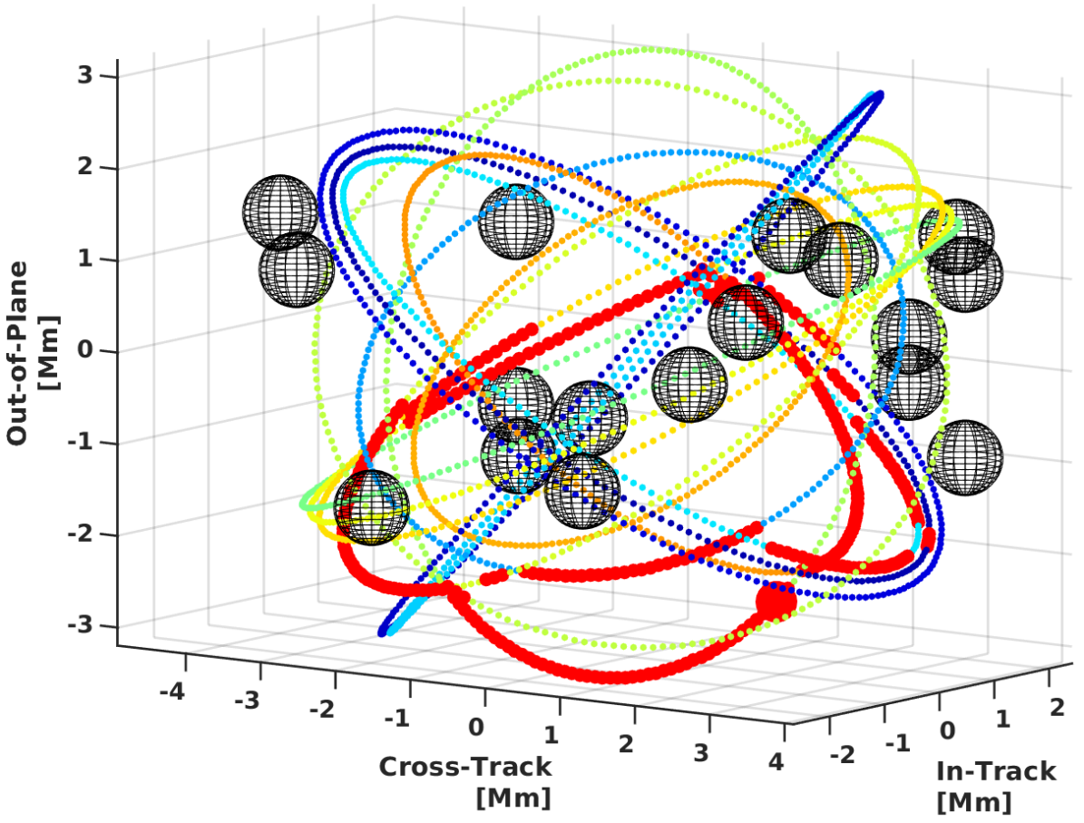
(a) Trajectory from a memoryless policy.

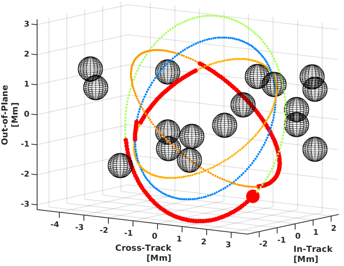
(b) Trajectory from policy with 5 memory states.

Figure 2: We show the obtained trajectory from a policy in red that finishes an orbit around the origin. We highlight the initial location by a big red circle. We depict the other objects by black spheres, and all NMTs that were used as a part of the trajectory.

Memory yields best policies.

Fig. 1(a) shows the convergence of the reachability probabilities for each model, specifically the probability versus the runtime in seconds. First, we observe that after 20 minutes of computation, using larger POMDPs that have a higher resolution or memory in the policy yields superior policies. Second, the policy with memory is superior to the policy without memory. Finally, we observe that larger models indeed require more time per iteration, which means that on the smaller uPOMDP S1, the algorithm converges faster to its optimum.

Comparing policies.

Fig. 2 shows a comparison of policies and depicts the resulting spacecraft trajectories. In particular, we show the trajectories from two different policies, a memoryless policy (one memory state) in Fig. 2(a) – computed on S1 – and from a policy with finite memory (five memory states) in Fig. 2(b) – computed on S2. The trajectory from the memoryless policy switches its orbit $17$ times, whereas the trajectory from the finite-memory policy switches its orbit only $4$ times. Additionally, the average length of the trajectory with the finite-memory policy is $188$, compared to $375$ for the memoryless one. These results demonstrate the utility of finite-memory to improve the reachability probability and minimize the number of switches.

Robust policies are more robust.

We demonstrate the utility of computing robust policies against uncertainty in Fig. 1(b). Intuitively, we compute policies on nominal models and use them on uncertain models. We give results on the nominal transition probabilities of the four considered models, where we ran Algorithm 1 on the nominal models until we reach the optimal value. The performance of the policies on the nominal models has solid lines, and the performance of the policies on the uncertain models has dashed lines. However, when we extract these policies and apply them on the uPOMDP, they perform significantly worse and fail to satisfy the objective in each case. The results clearly demonstrate the trade-offs between computing policies for nominal and uncertain problems. In each case, the computation time is roughly an order of magnitude larger. Yet, the resulting policies are better: we observe that the probability of a close encounter with another object increases up to $60$ percentage points, if we do not consider the uncertainty in the model.

Expected energy consumption.

Finally, we consider an example where there is a cost for switching orbits. The objective is to minimize the cost of successfully finishing a cycle in orbit. We obtain the cost of each switching action according to the parameters in (Frey et al. 2017). Additionally, we define the cost of a close encounter to be $10000N{\cdot}s$ (Newton-second, which is a unit for the impulse and relates to the fuel consumption), a much higher cost than all possible switching actions. We reduce the uncertainty in the model by setting the previously mentioned intervals for these models to $[0.90,0.95]$. In particular, the worst-case probability to correctly detect objects is now higher than before, reducing the probability of close encounters with those objects. Fig. 1(c) shows the convergence of the costs for each model. The costs of the resulting policies for models S1 and S2 are $178$ and $153N{\cdot}s,$ respectively. We ran into numerical troubles during the robust verification step for S3 and S4. Similar to the previous example, the results demonstrate the utility of finite-memory policies to reduce the fuel cost of spacecraft.

Aircraft Collision Avoidance

We consider robust aircraft collision avoidance (Kochenderfer 2015). The objective is to maximize the probability of avoiding a collision with an intruder aircraft while taking into account sensor errors and uncertainty in its future paths.

Figure 3: The probability of safely finishing the mission without collision in the aircraft collision example.

Model.

We consider a two-dimensional example with a state space consisting of (1) the own aircraft position $\langle x,y\rangle$ relative to the intruder, and (2) the relative speed of the intruder relative to the own aircraft, $\langle\dot{x},\dot{y}\rangle$. We (grid-)discretize the relative position in 900 cells of $\pm 100\times 100$ feet, and the relative speed in 100 cells of $\dot{x}$ and $\dot{y}$ variables into 10 points between $\pm 1000\times 1000$ feet/minute (in each direction). We use time steps of $1$ second. In each time step, the action choice reflects changing the acceleration of the own aircraft in two dimensions, while the intruder acceleration is chosen probabilistically. The state is then updated accordingly. The probabilistic changes by the intruder are given by uncertain intervals $I$, generalizing the model from (Kochenderfer 2015) where fixed values are assumed. We vary $I$ below. Additionally, the probability of the pilot being responsive at a given time is given by the interval $[0.70,0.90]$. The own aircraft cannot precisely observe the intruder’s position, and the accuracy of the observation is quantized by $\pm 300$ feet. The model has $476\,009$ states and $866\,889$ transitions. The specification is to maximize the probability of reaching the target while maintaining a distance of $\pm 400$ feet in either direction.

Variants.

We consider three ranges for intruder behavior in our example. The intruder A1 has an uncertain probability of applying an acceleration in one particular direction by the interval ${I=[0.2,0.8]}$, while we have ${I=[0.3,0,7]}$ and ${I=[0.4,0.6]}$ for A2 and A3, respectively.

Results.

We show the convergence of the method for each intruder in Fig. 3. We compute a locally optimal policy within minutes in each case. For the three models, the probability of satisfying the specification is $0.997$, $0.976$, and $0.76$, respectively. Last, we extract the policy to counter intruders within A3 and apply it to the uPOMDP defined for A1, which has more uncertainty than A3. Then, the resulting reachability probability is only $0.55$, which shows the utility of considering robustness against potentially adversarial intruders.

(a) On model S1

(b) On smaller models A4 and A5.

Figure 4: Comparing SCP with QCQP.

Comparing Performance

We compare our approach (SCP) with an implementation of (Suilen et al. 2020), based on an exponentially large quadratically constrained quadratic program (QCQP).

Let us first revisit the spacecraft problem. The QCQP method runs out of memory on all models except S1. For S1, QCQP indeed has a small advantage over SCP, cf. Fig. 4(a). We remark that the policies computed with SCP on S2, S3, and S4 are superior to the policy computed by QCQP on S1.

For the airplane problem, the QCQP again runs out of memory on A1, A2, and A3. For comparison, we construct models A4 and A5 by a coarser discretization (and varying uncertainty). The models have $18\,718$ states, and are smaller versions of A1 and A2. The performance is plotted in Fig. 4(b). For A4, QCQP yields a slightly better policy but takes more time, whereas, on A5, SCP finds a better policy faster.

We conclude that QCQP from (Suilen et al. 2020) is comparable on small models, but does not scale to large models.

7 Conclusion

We presented a new approach to computing robust policies for uncertain POMDPs. The experiments showed that we are able to apply our method based on convex optimization on well-known benchmarks with varying levels of uncertainty. Future work will involve incorporating learning-based techniques.

8 Acknowledgments

M. Cubuktepe and U. Topcu were supported in part by the grants ARL ACC-APG-RTP W911NF, NASA 80NSSC19K0209, and AFRL FA9550-19-1-0169. N. Jansen and M. Suilen were supported in part by the grants NWO OCENW.KLEIN.187: “Provably Correct Policies for Uncertain Partially Observable Markov Decision Processes”, NWA.1160.18.238: “PrimaVera”, and NWA.BIGDATA.2019.002: “EXoDuS - EXplainable Data Science”. S. Junges was supported in part by NSF grants 1545126 (VeHICaL) and 1646208, by the DARPA Assured Autonomy program, by Berkeley Deep Drive, and by Toyota under the iCyPhy center.

References

- Ahmadi et al. (2018) Ahmadi, M.; Cubuktepe, M.; Jansen, N.; and Topcu, U. 2018. Verification of Uncertain POMDPs Using Barrier Certificates. In Allerton, 115–122. IEEE.
- Alizadeh and Goldfarb (2003) Alizadeh, F.; and Goldfarb, D. 2003. Second-Order Cone Programming. Math Program. 95(1): 3–51.
- Amato, Bernstein, and Zilberstein (2010) Amato, C.; Bernstein, D. S.; and Zilberstein, S. 2010. Optimizing Fixed-size Stochastic Controllers for POMDPs and Decentralized POMDPs. AAMAS 21(3): 293–320.
- Ben-Tal, El Ghaoui, and Nemirovski (2009) Ben-Tal, A.; El Ghaoui, L.; and Nemirovski, A. 2009. Robust Optimization, volume 28. Princeton University Press.
- Bertsimas, Brown, and Caramanis (2011) Bertsimas, D.; Brown, D. B.; and Caramanis, C. 2011. Theory and Applications of Robust Optimization. SIAM review 53(3): 464–501.
- Burns and Brock (2007) Burns, B.; and Brock, O. 2007. Sampling-Based Motion Planning with Sensing Uncertainty. In ICRA, 3313–3318. IEEE.
- Chamie and Mostafa (2018) Chamie, M. E.; and Mostafa, H. 2018. Robust Action Selection in Partially Observable Markov Decision Processes with Model Uncertainty. In CDC, 5586–5591. IEEE.
- Chatterjee et al. (2016) Chatterjee, K.; Chmelík, M.; Gupta, R.; and Kanodia, A. 2016. Optimal Cost Almost-sure Reachability in POMDPs. Artif. Intell. 234: 26–48.
- Dehnert et al. (2017) Dehnert, C.; Junges, S.; Katoen, J.; and Volk, M. 2017. A Storm is Coming: A Modern Probabilistic Model Checker. In CAV (2), volume 10427 of LNCS, 592–600. Springer.
- Frey et al. (2017) Frey, G. R.; Petersen, C. D.; Leve, F. A.; Kolmanovsky, I. V.; and Girard, A. R. 2017. Constrained Spacecraft Relative Motion Planning Exploiting Periodic Natural Motion Trajectories and Invariance. Journal of Guidance, Control, and Dynamics 40(12): 3100–3115.
- Givan, Leach, and Dean (2000) Givan, R.; Leach, S.; and Dean, T. 2000. Bounded-Parameter Markov Decision Processes. Artif. Intell. 122(1-2): 71–109.
- Gurobi Optimization (2020) Gurobi Optimization, L. 2020. Gurobi Optimizer Reference Manual. URL http://www.gurobi.com.
- Hahn et al. (2017) Hahn, E. M.; Hashemi, V.; Hermanns, H.; Lahijanian, M.; and Turrini, A. 2017. Multi-Objective Robust Strategy Synthesis for Interval Markov Decision Processes. In QEST, volume 10503 of LNCS, 207–223. Springer.
- Hobbs and Feron (2020) Hobbs, K. L.; and Feron, E. M. 2020. A Taxonomy for Aerospace Collision Avoidance with Implications for Automation in Space Traffic Management. In AIAA Scitech 2020 Forum, 0877.
- Itoh and Nakamura (2007) Itoh, H.; and Nakamura, K. 2007. Partially Observable Markov Decision Processes with Imprecise Parameters. Artif. Intell. 171(8): 453 – 490.
- Junges et al. (2018) Junges, S.; Jansen, N.; Wimmer, R.; Quatmann, T.; Winterer, L.; Katoen, J.; and Becker, B. 2018. Finite-State Controllers of POMDPs using Parameter Synthesis. In UAI, 519–529.
- Kaelbling, Littman, and Cassandra (1998) Kaelbling, L. P.; Littman, M. L.; and Cassandra, A. R. 1998. Planning and Acting in Partially Observable Stochastic Domains. Artificial intelligence 101(1-2): 99–134.
- Kim et al. (2007) Kim, S. C.; Shepperd, S. W.; Norris, H. L.; Goldberg, H. R.; and Wallace, M. S. 2007. Mission Design and Trajectory Analysis for Inspection of a Host Spacecraft by a Microsatellite. In 2007 IEEE Aerospace Conference, 1–23. IEEE.
- Kochenderfer (2015) Kochenderfer, M. J. 2015. Decision Making Under Uncertainty: Theory and Application. MIT press.
- Lobo et al. (1998) Lobo, M. S.; Vandenberghe, L.; Boyd, S.; and Lebret, H. 1998. Applications of Second-Order Cone Programming. Linear Algebra and its Applications 284(1-3): 193–228.
- Madani, Hanks, and Condon (1999) Madani, O.; Hanks, S.; and Condon, A. 1999. On the Undecidability of Probabilistic Planning and Infinite-Horizon Partially Observable Markov Decision Problems. In AAAI, 541–548. AAAI Press.
- Mao et al. (2018) Mao, Y.; Szmuk, M.; Xu, X.; and Acikmese, B. 2018. Successive Convexification: A Superlinearly Convergent Algorithm for Non-convex Optimal Control Problems. arXiv preprint arXiv:1804.06539 .
- Meuleau et al. (1999) Meuleau, N.; Kim, K.-E.; Kaelbling, L. P.; and Cassandra, A. R. 1999. Solving POMDPs by Searching the Space of Finite Policies. In UAI, 417–426.
- Nilim and Ghaoui (2005) Nilim, A.; and Ghaoui, L. E. 2005. Robust Control of Markov Decision Processes with Uncertain Transition Matrices. Operations Research 53(5): 780–798.
- Osogami (2015) Osogami, T. 2015. Robust Partially Observable Markov Decision Process. In ICML, volume 37, 106–115.
- Puggelli et al. (2013) Puggelli, A.; Li, W.; Sangiovanni-Vincentelli, A. L.; and Seshia, S. A. 2013. Polynomial-Time Verification of PCTL Properties of MDPs with Convex Uncertainties. In CAV, volume 8044 of LNCS, 527–542. Springer.
- Puterman (1994) Puterman, M. L. 1994. Markov Decision Processes. John Wiley and Sons.
- Suilen et al. (2020) Suilen, M.; Jansen, N.; Cubuktepe, M.; and Topcu, U. 2020. Robust Policy Synthesis for Uncertain POMDPs via Convex Optimization. In IJCAI, 4113–4120. ijcai.org.
- Vlassis, Littman, and Barber (2012) Vlassis, N.; Littman, M. L.; and Barber, D. 2012. On the Computational Complexity of Stochastic Controller Optimization in POMDPs. ACM Trans. on Computation Theory 4(4): 12:1–12:8.
- Wiesemann, Kuhn, and Rustem (2013) Wiesemann, W.; Kuhn, D.; and Rustem, B. 2013. Robust Markov Decision Processes. Mathematics of Operations Research 38(1): 153–183.
- Wolff, Topcu, and Murray (2012) Wolff, E. M.; Topcu, U.; and Murray, R. M. 2012. Robust Control of Uncertain Markov Decision Processes with Temporal Logic Specifications. In CDC, 3372–3379. IEEE.
- Yuan (2015) Yuan, Y.-x. 2015. Recent Advances in Trust Region Algorithms. Mathematical Programming 151(1): 249–281.