A Wavelet-Based Independence Test for Functional Data with an Application to MEG Functional Connectivity

Abstract

Measuring and testing the dependency between multiple random functions is often an important task in functional data analysis. In the literature, a model-based method relies on a model which is subject to the risk of model misspecification, while a model-free method only provides a correlation measure which is inadequate to test independence. In this paper, we adopt the Hilbert-Schmidt Independence Criterion (HSIC) to measure the dependency between two random functions. We develop a two-step procedure by first pre-smoothing each function based on its discrete and noisy measurements and then applying the HSIC to recovered functions. To ensure the compatibility between the two steps such that the effect of the pre-smoothing error on the subsequent HSIC is asymptotically negligible, we propose to use wavelet soft-thresholding for pre-smoothing and Besov-norm-induced kernels for HSIC. We also provide the corresponding asymptotic analysis. The superior numerical performance of the proposed method over existing ones is demonstrated in a simulation study. Moreover, in an magnetoencephalography (MEG) data application, the functional connectivity patterns identified by the proposed method are more anatomically interpretable than those by existing methods.

Key Words: Reproducing kernel Hilbert space; Besov spaces; Permutation test; Human connectome project.

1 Introduction

In recent decades, functional data analysis (FDA) has been developed rapidly due to a huge and increasing number of datasets collected in the form of curves, surfaces and volumes. General introductions to the subject may be found in a few monographs (e.g., Ramsay and Silverman, 2005; Ferraty and Vieu, 2006). In many scientific fields, measurements are taken from multiple random functions per subject and the dependency between these functions is of interest. For instance, neuroscientists are interested in functional connectivity patterns between signals at multiple brain regions, which are measured over time in functional magnetic resonance imaging data. It is thus an important task in FDA to measure their dependency and to further test the significance of the dependency. Among extensive relevant research endeavors, most dependency test methods can be categorized as either model-based or model-free.

A model-based method typically infers the dependency between multiple functions by first assuming a functional regression model (see, e.g., Morris, 2015, for a survey) which characterizes their structural relationship, and then testing the significance of the assumed model. See examples of model-based methods by Guo (2002); Huang et al. (2002); Shen and Faraway (2004); Antoniadis and Sapatinas (2007) for concurrent/varying-coefficient models and by Kokoszka et al. (2008); Chen et al. (2020) for function-on-function regression models. The main disadvantage of a model-based method is its reliance on correct model specification. If the model is misspecified, the inference is not well grounded and might be inaccurate.

A model-free method can avoid the misspecification issue associated with model-based methods since it typically quantifies the dependency between random functions by a correlation measure, without assuming any particular model. As a natural extension of the canonical correlation for multivariate data, the functional canonical correlation is a popular correlation measure for functional data (e.g., Leurgans et al., 1993; He et al., 2003; Eubank and Hsing, 2008; Shin and Lee, 2015). However, it is plagued by the involvement of inverting a covariance operator, which is an ill-posed problem and often requires proper regularizations. The dynamical correlation (Dubin and Müller, 2005; Sang et al., 2019) and temporal correlation (Zhou et al., 2018) are two functional correlation measures without the aforementioned inverse problem. The former measures the angle between two random functions in the $L^{2}$ space. The latter essentially computes the Pearson correlation between two random functions at each time point and then averages all pointwise Pearson correlations over the time domain. However, since uncorrelatedness does not imply independence, these functional correlations are insufficient to test independence. Recently a few model-free approaches have been developed to test mean independence for functional data (e.g., Patilea et al., 2016; Lee et al., 2020), but they can only test a weaker notion of independence.

In this paper we develop a model-free independence test for functional data. Under the reproducing kernel Hilbert space (RKHS) framework, we propose to use the Hilbert-Schmidt Independence Criterion (HSIC, e.g., Gretton et al., 2005, 2008) to measure the dependency between two random functions. An appealing property is that HSIC is zero if and only if the two random functions are independent. However, the application of HSIC requires fully observed and noiseless functional data, while in practice functional data are always discretely measured and contaminated by noise. To tackle this problem, one may perform a two-step procedure: first pre-smooth the data, and then apply HSIC to the resulting functions. Clearly, pre-smoothing will affect the performance of HSIC. Indeed, the functional distance with respect to which the asymptotic convergence of the pre-smoothing procedure is measured is crucial, as HSIC is fundamentally based on a functional distance. Some common pre-smoothing procedures do not have existing convergence results on the required functional distance, and hence may not be compatible; namely, the pre-smoothing error may have a profound effect on the subsequent HSIC. See Section 3 for more discussion. In this work, we carefully design our procedure to ensure that the two steps are compatible. Our choice of the first step is wavelet soft-thresholding (e.g., Donoho et al., 1995), while the choice of HSIC is based on Besov-norm-induced kernels. We can show that these choices are theoretically compatible if the functional data are sufficiently densely measured. See Section 4 for details. This work is motivated by the Human Connectome Project (HCP, https://www.humanconnectome.org) from which various brain imaging datasets are publicly accessible. The application of our method to a magnetoencephalography (MEG) dataset from HCP is capable of identifying anatomically interpretable functional connectivity patterns. Therefore, the proposed method provides an important tool to study functional connectivity between different brain regions.

The main contribution of this paper is three-fold. First, we generalize HSIC to Besov spaces, a larger class of functions than Sobolev spaces which are popular in RKHS modeling. For random functions of which sample paths belong to Besov spaces, we show that the Besov sequence norm for their wavelet coefficients can induce a characteristic kernel, which is required by HSIC. Second, for dense functional data, we develop the asymptotic distribution of the empirical HSIC based on pre-smoothed functions by wavelet soft-thresholding. Since the asymptotic distribution involves many unknown quantities, we suggest a permutation test in practice and prove that not only can the test control the Type I error probability but also it is consistent. The theoretical results show that the two steps in our proposed procedure are compatible. Finally, we propose an data-adaptive approach to tuning the smoothness parameter for the Besov norm needed to induce the kernel for HSIC. It is numerically shown that this approach is able to enhance the sensitivity of HSIC to detecting dependencies at high frequencies.

The rest of the paper proceeds as follows. Section 2 provides a brief introduction to HSIC. The two-step procedure for the proposed wavelet-based HSIC test is given in Section 3. Its asymptotic properties are presented in Section 4. Section 5 provides a method for smoothness parameter selection. The numerical performance of the proposed method is illustrated in a simulation study in Section 6 and an MEG functional connectivity study in Section 7 where it is also compared with representative existing methods.

2 Hilbert-Schmidt Independence Criterion

In this section we give a brief introduction to HSIC. Let $X$ and $Y$ be two random functions of which sample paths belong to ${\mathcal{X}}$ and ${\mathcal{Y}}$ respectively, and ${{\mathcal{H}}(\kappa_{\mathcal{X}})}$ and ${{\mathcal{H}}(\kappa_{\mathcal{Y}})}$ be the RKHS equipped with kernels $\kappa_{\mathcal{X}}$ and $\kappa_{\mathcal{Y}}$ defined on ${\mathcal{X}}\times{\mathcal{X}}$ and ${\mathcal{Y}}\times{\mathcal{Y}}$ respectively.

HSIC requires that both $\kappa_{\mathcal{X}}$ and $\kappa_{\mathcal{Y}}$ are characteristic, in the sense that two probability measures $P=P^{\prime}$ if and only if ${\bf P}^{\kappa_{\mathcal{Z}}}(P)={\bf P}^{\kappa_{\mathcal{Z}}}(P^{\prime})$ where ${\bf P}^{\kappa_{\mathcal{Z}}}(P)=E_{P}\{\kappa_{\mathcal{Z}}(Z,\cdot)\}$ for a random function $Z\in{\mathcal{Z}}$ which follows $P$ and $(Z,{\mathcal{Z}})=(X,{\mathcal{X}})$ or $(Y,{\mathcal{Y}})$. A characteristic kernel may be induced by a strong negative type semi-metric (see Definition [S3] and Proposition [S1] in Appendix). Denote the joint probability measure of $X$ and $Y$ by $P_{XY}$ and their marginal probability measures by $P_{X}$ and $P_{Y}$ respectively. Since $\kappa_{\mathcal{X}}$ and $\kappa_{\mathcal{Y}}$ are characteristic, $P_{X}$ and $P_{Y}$ are fully characterized by ${\bf P}^{\kappa_{\mathcal{X}}}(P_{X})=E_{P_{X}}\{\kappa_{\mathcal{X}}(X,\cdot)\}$ and ${\bf P}^{\kappa_{\mathcal{Y}}}(P_{Y})=E_{P_{Y}}\{\kappa_{\mathcal{Y}}(Y,\cdot)\}$ respectively. Let ${\bf P}^{\kappa_{\mathcal{X}}\otimes\kappa_{\mathcal{Y}}}(P_{XY})=E_{P_{XY}}\{(\kappa_{\mathcal{X}}\otimes\kappa_{\mathcal{Y}})((X,Y),(*,\cdot))\}$, where the tensor product kernel $\kappa_{\mathcal{X}}\otimes\kappa_{\mathcal{Y}}$ is defined by $(\kappa_{\mathcal{X}}\otimes\kappa_{\mathcal{Y}})((x,y),(x^{\prime},y^{\prime}))=\kappa_{\mathcal{X}}(x,x^{\prime})\kappa_{\mathcal{Y}}(y,y^{\prime}),x,x^{\prime}\in{\mathcal{X}},y,y^{\prime}\in{\mathcal{Y}}$.

Sejdinovic et al. (2013) showed that $X$ and $Y$ are independent, i.e., $P_{XY}=P_{X}P_{Y}$, if and only if ${\bf P}^{\kappa_{\mathcal{X}}\otimes\kappa_{\mathcal{Y}}}(P_{XY})={\bf P}^{\kappa_{\mathcal{X}}}(P_{X}){\bf P}^{\kappa_{\mathcal{Y}}}(P_{Y})$, although $\kappa_{\mathcal{X}}\otimes\kappa_{\mathcal{Y}}$ is not characteristic for all probability measures on ${{\mathcal{H}}(\kappa_{\mathcal{Y}})}\times{{\mathcal{H}}(\kappa_{\mathcal{Y}})}$. Therefore, to test the independence between $X$ and $Y$, it suffices to study the difference between ${\bf P}^{\kappa_{\mathcal{X}}\otimes\kappa_{\mathcal{Y}}}(P_{XY})$ and ${\bf P}^{\kappa_{\mathcal{X}}}(P_{X}){\bf P}^{\kappa_{\mathcal{Y}}}(P_{Y})$. Since ${\bf P}^{\kappa_{\mathcal{X}}}(P_{X})\in{{\mathcal{H}}(\kappa_{\mathcal{X}})}$, ${\bf P}^{\kappa_{\mathcal{Y}}}(P_{Y})\in{{\mathcal{H}}(\kappa_{\mathcal{Y}})}$ and ${\bf P}^{\kappa_{\mathcal{X}}\otimes\kappa_{\mathcal{Y}}}(P_{XY})\in{{\mathcal{H}}(\kappa_{\mathcal{X}}\otimes\kappa_{\mathcal{Y}})}$ where ${{\mathcal{H}}(\kappa_{\mathcal{X}}\otimes\kappa_{\mathcal{Y}})}$ is the RKHS equipped with $\kappa_{\mathcal{X}}\otimes\kappa_{\mathcal{Y}}$, HSIC may be used to measure this difference under the norm of ${{\mathcal{H}}(\kappa_{\mathcal{X}}\otimes\kappa_{\mathcal{Y}})}$.

Definition 1 (HSIC).

Suppose that $\int\kappa_{\mathcal{X}}(x,x)dP_{X}(x)<\infty$ and $\int\kappa_{\mathcal{Y}}(y,y)dP_{Y}(y)<\infty$. The HSIC of $P_{XY}$ is defined by

$$\gamma(P_{XY},\kappa_{\mathcal{X}},\kappa_{\mathcal{Y}}) = \|{\bf P}^{\kappa_{\mathcal{X}}\otimes\kappa_{\mathcal{Y}}}(P_{XY})-{\bf P}^{\kappa_{\mathcal{X}}}(P_{X}){\bf P}^{\kappa_{\mathcal{Y}}}(P_{Y})\|_{{{\mathcal{H}}(\kappa_{\mathcal{X}}\otimes\kappa_{\mathcal{Y}})}}^{2}$$

$$= 4\iint\kappa_{\mathcal{X}}(x,x^{\prime})\kappa_{\mathcal{Y}}(y,y^{\prime})d(P_{XY}-P_{X}P_{Y})(x,y)d(P_{XY}-P_{X}P_{Y})(x^{\prime},y^{\prime}).$$

In practice with $\{(X_{i},Y_{i}):i=1,\ldots,n\}$ which are independently and identically distributed (i.i.d.) copies of $(X,Y)$, the sample versions of ${\bf P}^{\kappa_{\mathcal{X}}}(P_{X})$, ${\bf P}^{\kappa_{\mathcal{Y}}}(P_{Y})$ and ${\bf P}^{\kappa_{\mathcal{X}}\otimes\kappa_{\mathcal{Y}}}(P_{XY})$ are defined by ${\bf P}^{\kappa_{\mathcal{X}}}(P_{n,X})=n^{-1}\sum_{i=1}^{n}\kappa_{\mathcal{X}}(X_{i},\cdot)$, ${\bf P}^{\kappa_{\mathcal{Y}}}(P_{n,Y})=n^{-1}\sum_{i=1}^{n}\kappa_{\mathcal{Y}}(Y_{i},\cdot)$, and ${\bf P}^{\kappa_{\mathcal{X}}\otimes\kappa_{\mathcal{Y}}}(P_{n,XY})=n^{-1}\sum_{i=1}^{n}\{(\kappa_{\mathcal{X}}\otimes\kappa_{\mathcal{Y}})((X_{i},Y_{i}),(*,\cdot))\}.$ Obviously ${\bf P}^{\kappa_{\mathcal{X}}}(P_{n,X})\in{{\mathcal{H}}(\kappa_{\mathcal{X}})}$, ${\bf P}^{\kappa_{\mathcal{Y}}}(P_{n,Y})\in{{\mathcal{H}}(\kappa_{\mathcal{Y}})}$ and ${\bf P}^{\kappa_{\mathcal{X}}\otimes\kappa_{\mathcal{Y}}}(P_{n,XY})\in{{\mathcal{H}}(\kappa_{\mathcal{X}}\otimes\kappa_{\mathcal{Y}})}$, so we can obtain a sample version of HSIC as follows.

Definition 2 (Empirical HSIC).

Under the same setting in Definition 1, the empirical HSIC, which is an estimator of HSIC, is defined by

$$\gamma(P_{n,XY},\kappa_{\mathcal{X}},\kappa_{\mathcal{Y}})=\|{\bf P}^{\kappa_{\mathcal{X}}\otimes\kappa_{\mathcal{Y}}}(P_{n,XY})-{\bf P}^{\kappa_{\mathcal{X}}}(P_{n,X}){\bf P}^{\kappa_{\mathcal{Y}}}(P_{n,Y})\|_{{{\mathcal{H}}(\kappa_{\mathcal{X}}\otimes\kappa_{\mathcal{Y}})}}^{2}$$

$$=4\iint\kappa_{\mathcal{X}}(x,x^{\prime})\kappa_{\mathcal{Y}}(y,y^{\prime})d(P_{n,XY}-P_{n,X}P_{n,Y})(x,y)d(P_{XY}-P_{n,X}P_{n,Y})(x^{\prime},y^{\prime}).$$

By Sejdinovic et al. (2013), the empirical HSIC can be rewritten as

$$\gamma(P_{n,XY},\kappa_{\mathcal{X}},\kappa_{\mathcal{Y}})=n^{-2}\mbox{{\rm tr}}({\bm{\Gamma}^{X}}{\bf H}{\bm{\Gamma}^{Y}}{\bf H}),$$

where ${\bm{\Gamma}^{X}}=(\kappa_{\mathcal{X}}(X_{i},X_{j}))_{1\leq i,j\leq n}$ and ${\bm{\Gamma}^{Y}}=(\kappa_{\mathcal{Y}}(Y_{i},Y_{j}))_{1\leq i,j\leq n}$ are Gram matrices, and ${\bf H}={\bf I}_{n}-n^{-1}{\bf 1}_{n}{\bf 1}_{n}^{\top}$ is the centering matrix with the $n\times n$ identity matrix ${\bf I}_{n}$ and ${\bf 1}_{n}=(1,\ldots,1)^{\top}$ of dimension $n$.

3 Methodology

Suppose that bivariate functional data $\{(X_{i},Y_{i}):i=1,\ldots,n\}$ collected from $n$ subjects are i.i.d. copies of a pair of random functions $(X,Y)$, which, without loss of generality, is defined on the domain $[0,1]\times[0,1]$. Let the sample paths of $X$ and $Y$ belong to function spaces ${\mathcal{X}}$ and ${\mathcal{Y}}$ respectively. In many applications such as brain imaging analysis, the measurements of each function are sampled at a discrete and regular grid and subject to noise contamination. Hence we assume that the observations are $\{({\tilde{X}}_{il},{\tilde{Y}}_{il}):=(X_{i}(T_{l})+e_{il}^{X},Y_{i}(T_{l})+e_{il}^{Y}):i=1,\ldots,n;l=1,\ldots,m\},$ where $\{T_{l}=(l-1)/m:l=1,\ldots,m\}$ is a regular grid with $m=2^{J+1}$ for some integer $J>0$ and the two sets of i.i.d. mean-zero random noise $\{e_{il}^{X}:i=1,\ldots,n;l=1,\ldots,m\}$ and $\{e_{il}^{Y}:i=1,\ldots,n;l=1,\ldots,m\}$ with respective variances $\delta_{X}^{2}$ and $\delta_{Y}^{2}$ are independent of each other and of $\{(X_{i},Y_{i}):i=1,\ldots,n\}$. Our goal is to formulate an HSIC-based test for the independence between $X$ and $Y$ via $\{({\tilde{X}}_{il},{\tilde{Y}}_{il}):i=1,\ldots,n;l=1,\ldots,m\}$. For simplicity we assume that all functions share the same measurement grid and $m=2^{J+1}$, but the proposed method is applicable with minor modifications if the grid is irregular, the functions are measured at different grids, or $m\neq 2^{J+1}$ (see Remark 1).

Due to the success of existing HSIC-based independence tests for multivariate data, it is tempted to treat the discretized observations as multivariate data and directly apply existing methods. However, there are two issues with this approach. First, in order to capture enough information, $m$ should be large enough, which naturally leads to high-dimensional data. Without reasonable structure across these $m$ dimensions, HSIC does not perform well. In the FDA literature, modeling the sample paths with certain form of smoothness has been shown an empirically successful strategy in many applications. It is beneficial to incorporate smoothness structure during the design of a tailor-made HSIC method. Second, the discretized observations are contaminated by noise. Hence these raw observations are indeed not “smooth” but the noiseless ones are.

The proposed method is directly based on the definition of HSIC (Definition 1) when applied to random functions. Clearly, the application of such HSIC requires the trajectories of all random functions to be fully observed and noiseless. A natural idea is to perform pre-smoothing to recover these trajectories followed by an application of HSIC for random functions. However, the compatibility of these two steps is generally unclear. Namely, it is non-trivial to know whether the pre-smoothing error (measured in certain norm) would have a profound effect on the subsequent HSIC-based test. For instance, if the sample paths of all random functions are assumed to belong to a Sobolev space, it is seemingly reasonable to pre-smooth each trajectory by a smoothing spline followed by the HSIC based on Sobolev-norm-induced kernels. However, the compatibility of the two steps is unknown since there is no theoretical result to guarantee that the pre-smoothing error under a Sobolev norm converges to zero, although the corresponding results with respect to the $L^{2}$ or empirical norm exist.

To address this compatibility issue, we propose to use HSIC based on Besov-norm-induced kernels for testing independence under the assumption that the sample paths of all random functions belong to Besov spaces, a larger class of functions than Sobolev spaces. To recover each trajectory, we adopt wavelet soft-thresholding (Donoho et al., 1995), a successful pre-smoothing technique in Bosev spaces. Its theoretical compatibility with the proposed HSIC is given in Section 4. In the rest of this section, we first briefly introduce wavelets (e.g., Ogden, 1997; Vidakovic, 2009; Morettin et al., 2017) together with other related results and then give the details of the proposed two-step procedure.

3.1 Wavelets and Besov Sequence Norms

Following the Cohen-Daubechies-Jawerth-Vial (CDJV) construction (Cohen et al., 1993), let father and mother wavelets be $\phi,\psi\in C^{R}[0,1]$ respectively with $D$ vanishing moments (e.g., Daubechies, 1992) where $C^{R}[0,1]$ is the space of all functions on $[0,1]$ with $R$-th order continuous derivatives. We consider a Besov space $B_{p,q}^{\alpha}[0,1]$ with norm $\|\cdot\|_{B_{p,q}^{\alpha}[0,1]}$ of which smoothness parameter $\alpha$ satisfies $1/p<\alpha<\min\{R,D\}$ such that $B_{p,q}^{\alpha}[0,1]$ can be embedded continuously in $C[0,1]$. Formal definitions of $B_{p,q}^{\alpha}[0,1]$ and its norm $\|\cdot\|_{B_{p,q}^{\alpha}[0,1]}$ are given in Section [A.2] in Appendix. Then for any function $f\in B_{p,q}^{\alpha}[0,1]\cap L^{2}[0,1]$ and a fixed coarse scale $L$, we have the following decomposition

$$f(t)=\sum_{k=0}^{2^{L}-1}\xi_{k}\{2^{L/2}\phi(2^{L}t-k)\}+\sum_{j\geq L}\sum_{k=0}^{2^{j}-1}\theta_{j,k}\{2^{j/2}\psi(2^{j}t-k)\},\quad t\in[0,1].$$ (1)

Denote $\theta_{j,k}=\xi_{2^{j}+k},0\leq j<L,0\leq k<2^{j}$ and $\theta_{-1,0}=\xi_{0}$. Based on the wavelet coefficients of $f$, $\mbox{\boldmath$\theta$}^{f}=((\mbox{\boldmath$\theta$}_{-1}^{f})^{\top},(\mbox{\boldmath$\theta$}_{0}^{f})^{\top},\dots,(\mbox{\boldmath$\theta$}_{L}^{f})^{\top},(\mbox{\boldmath$\theta$}_{L+1}^{f})^{\top},\dots)^{\top}$ where $\mbox{\boldmath$\theta$}_{j}^{f}=(\theta_{j,0},\theta_{j,1},\dots,\theta_{j,2^{j}-1})^{\top}$ and $\mbox{\boldmath$\theta$}_{-1}^{f}=\theta_{-1,0}$, the Besov sequence norm $\|\cdot\|_{b_{p,q}^{\alpha}}$ (e.g., Donoho et al., 1995; Johnstone and Silverman, 2005) is defined by

$$\|\mbox{\boldmath$\theta$}^{f}\|_{b_{p,q}^{\alpha}}=\left(\sum_{j\geq-1}2^{jsq}\|\mbox{\boldmath$\theta$}_{j}^{f}\|_{p}^{q}\right)^{1/q},\quad s=\alpha+1/2-1/p,$$

where $\|\cdot\|_{p}$ refers to the $\ell_{p}$-norm for vectors. Denote the corresponding space by $b_{p,q}^{\alpha}=\{{\bf a}:\|{\bf a}\|_{b_{p,q}^{\alpha}}<\infty\}$. Note that the two norms $\|\cdot\|_{B_{p,q}^{\alpha}}$ and $\|\cdot\|_{b_{p,q}^{\alpha}}$ are equivalent (e.g., DeVore and Lorentz, 1993; Donoho et al., 1995) and obviously $b_{p,q}^{\alpha}\subset b_{p,q}^{\beta}$ if $\beta\leq\alpha$.

We can show that some Besov sequence norm can induce a characteristic kernel, which is required by HSIC.

Theorem 1.

For $0<q\leq p\leq 2$ and $\alpha>0$, let the semi-metric $\rho_{b_{p,q}^{\alpha}}(f,g)=\|\mbox{\boldmath$\theta$}^{f}-\mbox{\boldmath$\theta$}^{g}\|_{b_{p,q}^{\alpha}}^{q}$ for $f,g\in B_{p,q}^{\alpha}[0,1]$ where $\mbox{\boldmath$\theta$}^{f}$ and $\mbox{\boldmath$\theta$}^{g}$ are the wavelet coefficients of $f$ and $g$ respectively. The kernel induced by $\rho_{b_{p,q}^{\alpha}}$, which is $\kappa\left(z,z^{\prime}\right)=\rho_{b_{p,q}^{\alpha}}(z,0)+\rho_{b_{p,q}^{\alpha}}\left(z^{\prime},0\right)-\rho_{b_{p,q}^{\alpha}}\left(z,z^{\prime}\right)$, $z,z^{\prime}\in B_{p,q}^{\alpha}[0,1]$, is symmetric, positive definite and characteristic.

The proof of Theorem 1 is given in Section [B.1] in Appendix. By Theorem 1, we can define HSIC properly based on kernels induced by Besov sequence norms. For simplicity, hereafter we focus on popular choices of $p=q=2$. Accordingly we abbreviate $B_{2,2}^{\alpha}[0,1]$ and $b_{2,2}^{\alpha}$ to $B^{\alpha}$ and $b^{\alpha}$ respectively.

3.2 Two-Step Procedure

Under the setting in Section 3.1, we assume $X\in B^{\alpha_{X}}$ and $Y\in B^{\alpha_{Y}}$ where $1/2<\alpha_{X},\alpha_{Y}<\min\{R,D\}$. To test the independence between $X$ and $Y$ based on their discretely measured and noisy observations, we propose to first denoise each function and then apply HSIC to the recovered functions. The two-step procedure is explicitly stated as follows:

Step 1

By the decomposition (1) and the resolution limitation due to a finite number of measurements $m=2^{J+1}$ taken for each subject, we first obtain the initial wavelet coefficient estimates for each $X_{i}$, denoted by $\mbox{\boldmath$\theta$}^{{\tilde{X}}_{i}}=((\mbox{\boldmath$\theta$}_{-1}^{{\tilde{X}}_{i}})^{\top},(\mbox{\boldmath$\theta$}_{0}^{{\tilde{X}}_{i}})^{\top},\dots,(\mbox{\boldmath$\theta$}_{J}^{{\tilde{X}}_{i}})^{\top})^{\top}$ by the discrete wavelet transformation with the coarse scale $L_{X}$. The coarse scale $L_{X}$ may be selected by cross-validation or domain knowledge. Then we denoise each $\mbox{\boldmath$\theta$}^{{\tilde{X}}_{i}}$ by wavelet soft-thresholding (Donoho et al., 1995). Explicitly, the soft-thresholded estimates $\mbox{\boldmath$\theta$}^{{\hat{X}}_{i}}=((\mbox{\boldmath$\theta$}_{-1}^{{\hat{X}}_{i}})^{\top},(\mbox{\boldmath$\theta$}_{0}^{{\hat{X}}_{i}})^{\top},\dots,(\mbox{\boldmath$\theta$}_{J}^{{\hat{X}}_{i}})^{\top})^{\top}$ are obtained by $\mbox{\boldmath$\theta$}_{j}^{{\hat{X}}_{i}}=\mbox{\boldmath$\theta$}_{j}^{{\tilde{X}}_{i}}$, $j=-1,\dots,L_{X}-1$ and $\mbox{\boldmath$\theta$}_{j}^{{\hat{X}}_{i}}=\{\mbox{{\rm sgn}}(\theta_{j,k}^{{\tilde{X}}_{i}})\left(|\theta_{j,k}^{{\tilde{X}}_{i}}|-\delta_{X}\sqrt{(2\log m)/m}\right)_{+}:k=0,\ldots,2^{j}-1\}$, $j=L_{X},\ldots,J$, where $(x)_{+}=\max\{x,0\}$ and $\delta_{X}$ is the noise standard deviation. We denote each denoised function by ${\hat{X}}_{i}$, $i=1,\ldots,n$. To estimate $\delta_{X}$, we adopt the robust estimator (Donoho et al., 1995) $\hat{\delta}_{X}=\text{median}\left\{\sqrt{m}\theta_{J,k}^{{\tilde{X}}_{i}}:k=0,\dots,2^{J}\right\}/\text{median}(\left|W\right|)$, where $W$ is a standard normal random variable. We can similarly obtain $\mbox{\boldmath$\theta$}^{{\hat{Y}}_{i}}$ and ${\hat{Y}}_{i}$, $i=1,\ldots,n$.

Step 2

Since the soft-thresholded wavelet coefficient estimates $\mbox{\boldmath$\theta$}^{{\hat{X}}_{i}}\in b^{\alpha_{X}}\subset b^{\beta_{X}}$ and $\mbox{\boldmath$\theta$}^{{\hat{Y}}_{i}}\in b^{\alpha_{Y}}\subset b^{\beta_{Y}}$, $i=1,\ldots,n$, for any $\beta_{X}<\alpha_{X}$ and $\beta_{Y}<\alpha_{Y}$, we may apply HSIC to the denoised functions where the kernels $\kappa_{\mathcal{X}}$ and $\kappa_{\mathcal{Y}}$ are induced by $\rho_{b^{\beta_{X}}}$ and $\rho_{b^{\beta_{Y}}}$ respectively as defined in Theorem 1. Explicitly, we have $\gamma(P_{n,{\hat{X}}{\hat{Y}}},\kappa_{\mathcal{X}},\kappa_{\mathcal{Y}})=n^{-2}\mbox{{\rm tr}}({\bm{\Gamma}^{{\hat{X}}}}{\bf H}{\bm{\Gamma}^{{\hat{Y}}}}{\bf H}),$ where

$${\bm{\Gamma}^{{\hat{X}}}} =\left(\|\mbox{\boldmath$\theta$}^{{\hat{X}}_{i}}\|_{b^{\beta_{X}}}^{2}+\|\mbox{\boldmath$\theta$}^{{\hat{X}}_{j}}\|_{b^{\beta_{X}}}^{2}-\|\mbox{\boldmath$\theta$}^{{\hat{X}}_{i}}-\mbox{\boldmath$\theta$}^{{\hat{X}}_{j}}\|_{b^{\beta_{X}}}^{2}\right)_{1\leq i,j\leq n},\quad\mbox{and}$$

$${\bm{\Gamma}^{{\hat{Y}}}} =\left(\|\mbox{\boldmath$\theta$}^{{\hat{Y}}_{i}}\|_{b^{\beta_{Y}}}^{2}+\|\mbox{\boldmath$\theta$}^{{\hat{Y}}_{j}}\|_{b^{\beta_{Y}}}^{2}-\|\mbox{\boldmath$\theta$}^{{\hat{Y}}_{i}}-\mbox{\boldmath$\theta$}^{{\hat{Y}}_{j}}\|_{b^{\beta_{Y}}}^{2}\right)_{1\leq i,j\leq n}.$$

By adopting $\rho_{b^{\beta_{X}}}$ and $\rho_{b^{\beta_{Y}}}$ where $\beta_{X}<\alpha_{X}$ and $\beta_{Y}<\alpha_{Y}$ to construct kernels, we are able to make the pre-smoothing step theoretically compatible with the HSIC. As revealed in Lemma 1 and Theorem 2 in Section 4 below, if the observations of all functions are sufficiently dense, the denoising error due to wavelet soft-thresholding is asymptotically negligible in the asymptotic distribution of the HSIC. This is a key benefit of using wavelets and Besov norms for pre-smoothing.

In Section 4, the asymptotic distribution of $\gamma(P_{n,{\hat{X}}{\hat{Y}}},\kappa_{\mathcal{X}},\kappa_{\mathcal{Y}})$ is developed in Theorem 2 under the independence hypothesis. Despite its theoretical appeal, the asymptotic distribution unfortunately involves many unknown quantities. Therefore, we suggest using permutations to perform the independence test which, as shown in Theorem 3, can control the Type I error probability and is also consistent.

Remark 1.

Since denoising is performed separately for each function and subject, the proposed method is applicable when the functions of different subjects are not measured at the same grid. For $m\neq 2^{J+1}$ at fixed but possibly irregular designs, resampling or linear interpolation may be applied if the original measurement resolution is sufficiently high (e.g. Kovac and Silverman, 2000). For random designs with different measurements per subject, one may apply the method by Cai and Brown (1999) or by Pensky and Vidakovic (2001).

4 Asymptotic Theory

In this section we show that the proposed two-step procedure can lead to an asymptotically valid test, which addresses the compatibility issue raised in Section 3. Explicitly, we first provide the rate of convergence for the denoising error involved in Step 1 in Lemma 1, then the asymptotic distribution of HSIC $\gamma(P_{n,{\hat{X}}{\hat{Y}}},\kappa_{\mathcal{X}},\kappa_{\mathcal{Y}})$ in Step 2 in Theorem 2, and finally the asymptotic properties of the permutation test in Theorem 3. Hereafter, the kernels $\kappa_{\mathcal{X}}$ and $\kappa_{\mathcal{Y}}$ are induced by $\rho_{b^{\beta_{X}}}$ and $\rho_{b^{\beta_{Y}}}$ respectively.

Lemma 1.

Let $Z=X$ or $Y$. Assume that the noise $e_{il}^{Z}\sim N(0,\delta_{Z}^{2}),i=1,\ldots,n,l=1,\ldots,m$, $\beta_{Z}<\alpha_{Z}$, and $\|\mbox{\boldmath$\theta$}^{Z}\|_{b^{\alpha_{Z}}}\leq C_{Z}$ for a constant $C_{Z}>0$. Then as $m\rightarrow\infty$,

$$\|\mbox{\boldmath$\theta$}^{\hat{Z}_{i}}-\mbox{\boldmath$\theta$}^{Z_{i}}\|_{b^{\beta_{Z}}}=O_{p}\left\{m^{-r_{1}^{Z}/2}(\log m)^{r_{1}^{Z}/2+r_{2}^{Z}}\right\},\quad\text{uniformly for $i=1,\ldots,n$,}$$

where $r_{1}^{Z}=(\alpha_{Z}-\beta_{Z})/(\alpha_{Z}+1/2)$ and $r_{2}^{Z}=(1/2)\cdot I(0\leq\beta_{Z}\leq 1/2)$.

Lemma 1 is a special case of Theorem 4 in Donoho et al. (1995) so its proof is omitted. All assumptions in Lemma 1 are standard in the literature of wavelet soft-thresholding (e.g. Donoho et al., 1995; Johnstone and Silverman, 2005). Lemma 1 indicates that the denoising error converges to zero if the functional data are sufficiently densely measured.

Since the HSIC is constructed based on the kernels induced by $\rho_{b^{\beta_{X}}}$ and $\rho_{b^{\beta_{Y}}}$, the same norms used to evaluate the denoising error as in Lemma 1, the compatibility between the pre-smoothing by wavelet soft-thresholding and HSIC is theoretically guaranteed. As shown in Theorem 2, the effect of the denosing error on the distribution of the HSIC is asymptotically negligible for dense functional data.

To develop the asymptotic distribution of $\gamma(P_{n,{\hat{X}}{\hat{Y}}},\kappa_{\mathcal{X}},\kappa_{\mathcal{Y}})$, we further define the centered kernel for $\kappa_{\mathcal{X}}$ by ${\check{\kappa}_{\mathcal{X}}}(X,{X^{\prime}})=\langle\kappa_{\mathcal{X}}(X,\cdot)-\mu_{\kappa_{\mathcal{X}}}(P_{X}),\kappa_{\mathcal{X}}({X^{\prime}},\cdot)-\mu_{\kappa_{\mathcal{X}}}(P_{X})\rangle_{{{\mathcal{H}}(\kappa_{\mathcal{X}})}},$ where $\mu_{\kappa_{\mathcal{X}}}(P_{X})=\int\kappa_{\mathcal{X}}(x,\cdot)dP_{X}(x)$. Furthermore define an integral kernel operator $S_{{\check{\kappa}_{\mathcal{X}}}}:{{\mathcal{H}}(\kappa_{\mathcal{X}})}\rightarrow{{\mathcal{H}}(\kappa_{\mathcal{X}})}$ by $S_{{\check{\kappa}_{\mathcal{X}}}}(g)=\int_{{\mathcal{X}}}{\check{\kappa}_{\mathcal{X}}}(x,\cdot)g(x)dP_{X}$ for any $g\in{{\mathcal{H}}(\kappa_{\mathcal{X}})}$. An integral kernel operator $S_{{\check{\kappa}_{\mathcal{Y}}}}$ for $Y$ can be similarly defined.

Theorem 2.

Under the same assumptions of Lemma 1, if $m$ satisfies

$$m^{-r_{1}^{Z}/2}(\log m)^{r_{1}^{Z}/2+r_{2}^{Z}}=o(n^{-1/2}),$$ (2)

where $r_{1}^{Z}=(\alpha_{Z}-\beta_{Z})/(\alpha_{Z}+1/2)$ and $r_{2}^{Z}=(1/2)\cdot I(0\leq\beta_{Z}\leq 1/2)$, for $Z=X$ or $Y$, then

$$n\gamma(P_{n,{\hat{X}}{\hat{Y}}},\kappa_{\mathcal{X}},\kappa_{\mathcal{Y}})\rightsquigarrow\begin{cases}\sum_{r=1}^{\infty}\sum_{s=1}^{\infty}\mu_{r}\nu_{s}N_{rs}^{2},&\text{if $X$ and $Y$ are independent},\\ \infty,&\text{otherwise},\end{cases}$$

where “$\rightsquigarrow$” represents weak convergence, $N_{rs}\sim N(0,1),r,s\geq 1$ are i.i.d. and $\left\{\mu_{r}:r\geq 1\right\}$ and $\left\{\nu_{s}:s\geq 1\right\}$ are eigenvalues of $S_{{\check{\kappa}_{\mathcal{X}}}}$ and $S_{{\check{\kappa}_{\mathcal{Y}}}}$ respectively.

The proof of Theorem 2 is given in Section [B.2] in Appendix. The asymptotic distribution of $\gamma(P_{n,{\hat{X}}{\hat{Y}}},\kappa_{\mathcal{X}},\kappa_{\mathcal{Y}})$ in Theorem 2 is the same as that for fully observed $\{(X_{i},Y_{i}):X_{i}\in B^{\beta_{X}},Y_{i}\in B^{\beta_{Y}},i=1,\ldots,n\}$ (Sejdinovic et al., 2013). The requirement (2) ensures that the error due to wavelet soft-thresholding is asymptotically negligible under $b^{\beta_{Z}}$ norm if the measurements are sufficiently dense. In general, for fixed $\alpha_{Z}$ and $\beta_{Z}$, the order of $m$ should be higher than $n^{1/r_{Z}}$, which, for example, is $n^{7/4}$ if $(\alpha_{Z},\beta_{Z})=(3,1)$ and $n^{5/3}$ if $(\alpha_{Z},\beta_{Z})=(2,1/2)$.

Since the asymptotic reference distribution of $\gamma(P_{n,{\hat{X}}{\hat{Y}}},\kappa_{\mathcal{X}},\kappa_{\mathcal{Y}})$ when $X$ and $Y$ are assumed independent involves many unknown quantities, in practice we perform the test by permutation. As shown in Theorem 3, the permutation test can control the Type I error probability and is also consistent.

Theorem 3 (Permutation Test).

Let the level of significance be $\alpha\in(0,1)$. If the null hypothesis that $X$ and $Y$ are independent is true, the permutation test of $\gamma(P_{n,{\hat{X}}{\hat{Y}}},\kappa_{\mathcal{X}},\kappa_{\mathcal{Y}})$ based on a finite number of permutations rejects the null hypothesis with probability at most $\alpha$. If the alternative hypothesis that $X$ and $Y$ are dependent is true and the assumptions of Lemma 1 and (2) hold, the permutation test of $\gamma(P_{n,{\hat{X}}{\hat{Y}}},\kappa_{\mathcal{X}},\kappa_{\mathcal{Y}})$ based on $B\geq 1/\alpha-1$ permutations is consistent, i.e., $P(\hat{p}_{{\hat{X}}{\hat{Y}}}\leq\alpha)\rightarrow 1$ as $n\rightarrow\infty$, where $\hat{p}_{{\hat{X}}{\hat{Y}}}$ is the p-value.

The proof of Theorem 3 is given in Section [B.3] in Appendix. Theorem 3 shows that the proposed permutation test is also theoretically compatible with the wavelet soft-thresholding denoising.

5 Tuning Parameter Selection

The proposed method in Section 3 requires a proper choice of tuning parameters $\beta_{X}$ and $\beta_{Y}$. In this section we first discuss their roles in dependency detection and then propose a data-adaptive selection method for them.

In Section 4, Lemma 1 seems to imply that given $\alpha_{X}$ and $\alpha_{Y}$, the best choice is $\beta_{X}=\beta_{Y}=0$ because the corresponding denoising error attains the best rate of convergence. However, this choice of $\beta_{X}$ and $\beta_{Y}$ may result in a poor dependency detection especially when the dependency of $X$ and $Y$ originates from their high frequency bands.

For illustration, by Definition 1 and (3.1), we have the following decomposition

$$\gamma(P_{XY},\kappa_{\mathcal{X}},\kappa_{\mathcal{Y}}) =\gamma\Big{(}P_{XY},\sum_{j_{X}\geq-1}2^{2\beta_{X}j_{X}}\kappa_{\mathcal{X}}^{(j_{X})},\sum_{j_{Y}\geq-1}2^{2\beta_{Y}j_{Y}}\kappa_{\mathcal{Y}}^{(j_{Y})}\Big{)}$$

$$=\sum_{j_{X}\geq-1}\sum_{j_{Y}\geq-1}\gamma\Big{(}P_{XY},2^{2\beta_{X}j_{X}}\kappa_{\mathcal{X}}^{(j_{X})},2^{2\beta_{Y}j_{Y}}\kappa_{\mathcal{Y}}^{(j_{Y})}\Big{)},$$

where $\kappa_{\mathcal{Z}}^{(j_{Z})}(z,z^{\prime})=\|\mbox{\boldmath$\theta$}_{j}^{z}\|_{2}^{2}+\|\mbox{\boldmath$\theta$}_{j}^{z^{\prime}}\|_{2}^{2}-\|\mbox{\boldmath$\theta$}_{j}^{z}-\mbox{\boldmath$\theta$}_{j}^{z^{\prime}}\|_{2}^{2}$ for $j_{Z}\geq-1$, with $(z,Z,{\mathcal{Z}})=(x,X,{\mathcal{X}})$ or $(y,Y,{\mathcal{Y}})$ and Euclidean norm $\|\cdot\|_{2}$. Apparently $\gamma\Big{(}P_{XY},2^{2\beta_{X}j_{X}}\kappa_{\mathcal{X}}^{(j_{X})},2^{2\beta_{Y}j_{Y}}\kappa_{\mathcal{Y}}^{(j_{Y})}\Big{)}$ measures the dependency contribution to the HSIC at $j_{X}$ and $j_{Y}$ of $X$ and $Y$ respectively, which is zero if and only if $X$ and $Y$ are independent at $j_{X}$ and $j_{Y}$. If $\beta_{X}=\beta_{Y}=0$, the scaling factors $2^{\beta_{X}j_{X}}=2^{\beta_{Y}j_{Y}}=1$ for all $j_{X}\geq-1,j_{Y}\geq-1$ and it will be very difficult to detect the dependency between $X$ and $Y$ at high frequencies since the dependency contributions contained at high frequencies are very likely to be overwhelmed by the independent signals at low frequencies. Therefore, we aim to select $\beta_{X}$ and $\beta_{Y}$ such that the dependency contributions at high frequencies, if any, are detectable.

The idea of the proposed tuning method is to balance the dependency contributions to HSIC at all frequency scales such that they are approximately the same. To lessen the computational burden, a marginal selection algorithm is proposed in the sense that the optimal $\beta_{X}$ is selected only based on $X$ without reliance on $Y$. Note that, by the Cauchy-Schwarz inequality, the dependency contribution at each $j_{X},j_{Y}\geq-1$ satisfies

$$\gamma\Big{(}P_{XY},2^{2\beta_{X}j_{X}}\kappa_{\mathcal{X}}^{(j_{X})},2^{2\beta_{Y}j_{Y}}\kappa_{\mathcal{Y}}^{(j_{Y})}\Big{)} \leq 2^{2(\beta_{X}j_{X}+\beta_{Y}j_{Y})}\sqrt{\gamma(P_{X},\kappa_{\mathcal{X}}^{(j_{X})})\gamma(P_{Y},\kappa_{\mathcal{Y}}^{(j_{Y})})},$$

where $\gamma(P_{Z},\kappa_{\mathcal{Z}}^{(j_{Z})})=4\iint\kappa_{\mathcal{Z}}^{(j_{Z})}(z,z^{\prime})^{2}d(P_{Z}-P_{Z}^{2})(z)d(P_{Z}-P_{Z}^{2})(z^{\prime}),$ $j_{Z}\geq-1,$ is essentially a distance variance (Székely et al., 2007) with $(z,Z,{\mathcal{Z}})=(x,X,{\mathcal{X}})$ or $(y,Y,{\mathcal{Y}})$ (Sejdinovic et al., 2013). Thus we propose to select $\beta_{X}$ by balancing $2^{2\beta_{X}j_{X}}\sqrt{\gamma(P_{X},\kappa_{\mathcal{X}}^{(j_{X})})}$ at all $j_{X}\geq-1$. If $2^{2\beta_{X}j_{X}}\sqrt{\gamma(P_{X},\kappa_{\mathcal{X}}^{(j_{X})})}\approx C$ where $C>0$ is a constant, then $2\beta_{X}j_{X}+\frac{1}{2}\log_{2}\gamma(P_{X},\kappa_{\mathcal{X}}^{(j_{X})})\approx\log_{2}C,$ so $\beta_{X}$ may be selected as the estimated slope of the linear regression on $(-2j_{X},\log_{2}\gamma(P_{X},\kappa_{\mathcal{X}}^{(j_{X})})/2)$.

In practice, we could estimate $\gamma(P_{X},\kappa_{\mathcal{X}}^{(j_{X})})$ by $\gamma(P_{n,{\hat{X}}},\kappa_{\mathcal{X}}^{(j_{X})})$ for each $j_{X}\geq-1$, but its accuracy is poor for very high frequencies due to noise contamination. Thus we only consider $j_{X}$ up to $\overline{j}_{X}=\max_{j_{X}\geq L_{X}}\{\gamma(P_{n,{\hat{X}}},\kappa_{\mathcal{X}}^{(j_{X})})\geq\gamma(P_{n,\hat{e}^{X}},\kappa_{\mathcal{X}}^{(j_{X})})\}$ where $\hat{e}^{X}={\tilde{X}}-{\hat{X}}$ is the residual, such that the distance variances of all $j_{X}\leq\overline{j}_{X}$ are not smaller than that of the residual. If a known frequency band is of interest in the context of a study, e.g., the alpha band of brain signals, one may alternatively select $\beta_{X}$ by balancing $2^{2\beta_{X}j_{X}}\sqrt{\gamma(P_{X},\kappa_{\mathcal{X}}^{(j_{X})})}$ over that frequency band. Last, we remark that the computational benefit of the proposed marginal approach for tuning parameter selection is substantial when many tests have to be performed, such as in the functional connectivity analysis (Section 7).

6 Simulation

In this section we evaluate the numerical performance of our proposed wavelet-based HSIC method wavHSIC in both controlling the Type I error probability and statistical power. We also compare it with a few representative existing methods, including

1. Pearson Correlation (Pearson). It is a one-sample t-test based on Fisher-Z transformed correlation coefficients of all subjects. The correlation coefficient for each subject is obtained by applying the Pearson correlation formula to the bivariate time series of the subject, without adjusting for any possible dependence within the time series. It is a popular functional connectivity measure in neuroscience (e.g., He et al., 2012).

2. Dynamical Correlation (dnm, Dubin and Müller, 2005). It is defined as the expectation of the cosine of the $L^{2}$ angle between the standardized versions of two random functions.

3. Global Temporal Correlation (gtemp, Zhou et al., 2018). It is the integral of the Pearson correlation obtained at each time point.

4. Bias-Corrected Distance Covariance (dCov-c, Székely and Rizzo, 2013). It is a t-test designed to correct the bias of distance covariance for high-dimensional multivariate data. We apply it by treating the discrete measurements of two random functions as multivariate data. If the bias is not corrected, it is equivalent to wavHSIC with $\beta_{X}=\beta_{Y}=0$.

5. FPCA-Based Distance Covariance (FPCA, Kosorok, 2009). The distance covariance (Székely et al., 2007) is applied to top FPC scores which cumulatively account for 95% of the variation of each random function. When all FPC scores are used, it is equivalent to wavHSIC when $\beta_{X}=\beta_{Y}=0$.

6. Functional Linearity Test (KMSZ, Kokoszka et al., 2008). It is an approximate chi-squared test for the nullity of the coefficient function by assuming a functional linear model between the two random functions. The model fitting requires a satisfactory approximation of each random function by its top FPC scores and we select those which cumulatively account for 95% of variation of each random function.

The first five in comparison are model-free methods while the last is one of the most popular model-based methods in the FDA literature. Permutation is used to obtain the p-value for testing independence for wavHSIC, dnm, gtemp and FPCA.

We generated $199$ simulated datasets, where the specific choice $199$ is chosen to prevent empirical Type I and Type II error probabilities from coinciding with the level of significance $0.05$. In each simulated dataset $n=50$ or $200$ independent subjects with bivariate functions $\{(X_{i}(t),Y_{i}(t)):t\in[0,1],i=1,\ldots,n\}$ were generated where for the $i$-th subject, $X_{i}(t)=\sum_{k=1}^{16}\eta_{ik}\phi_{k}(t)$ and $Y_{i}(t)=\sum_{k=1}^{16}\zeta_{ik}\phi_{k}(t+0.2)$ with $\phi_{2k-1}(t)=\sqrt{2}\cos(2\pi kt),\phi_{2k}(t)=\sqrt{2}\sin(2\pi kt)$ for $k=1,\dots,8$. We considered three settings with different dependency structures of the bivariate functional data which are controlled by the FPC scores $\{(\eta_{ik},\zeta_{ik}):k=1,\dots,16;i=1,\dots,n\}$.

• Setting 1. We generated $\eta_{ik}\sim N(0,k^{-1.05}),k=1,\ldots,16$ and $\zeta_{ik}\sim N(0,k^{-1.2}),k=1,\ldots,16$ independently.

• Setting 2. With $\rho=0$ for $k=1,\dots,8$ and $\rho=0.6$ for $k=9,\dots,16$, we generated

  $$\begin{bmatrix}\eta_{ik}\\ \zeta_{ik}\end{bmatrix}\sim N\left(\begin{bmatrix}0\\ 0\end{bmatrix},\begin{bmatrix}k^{-1.05}&\rho k^{-1.125}\\ \rho k^{-1.125}&k^{-1.2}\end{bmatrix}\right).$$

• Setting 3. For $k=1,\dots,8$, $\eta_{ik}\sim N(0,k^{-1.05})$ was generated independently of $\zeta_{ik}\sim N(0,k^{-1.2})$. For $k=9,\dots,16$, $\eta_{ik}\sim N(0,k^{-1.05})$ and $\zeta_{ik}=\eta_{ik}^{2}-\mbox{{\rm E}}\eta_{ik}^{2}$.

Apparently $X$ and $Y$ are independent in Setting 1 and dependent in Settings 2 and 3. In Setting 2, the FPC scores of $X$ and $Y$ are linearly correlated but only at high spectral frequencies, while in Setting 3 they are linearly uncorrelated but dependent only at high spectral frequencies, so it is more difficult to detect dependency for all methods in Setting 3 than Setting 2.

Both functions are measured at $m=64$ or $256$ equidistant points on the time domain $[0,1]$. We added Gaussian noise to all measurements with signal-to-noise ratio $\text{SNR}=4$ or $8$, which is the variance of all measurements over the noise variance.

Since all six methods in comparison require noiseless functions, we used the same denoising approach for all of them for fairness. Explicitly, we denoised each curve by the empirical Bayes wavelet soft-thresholding method (Johnstone and Silverman, 2005) in the R package wavethresh. For wavHSIC, we chose the CDJV wavelet basis functions with vanishing moment $D=10$ for both $X$ and $Y$, which leads to $\alpha_{X}=\alpha_{Y}\approx 2.902$ (Daubechies, 1992). The tuning parameters $\beta_{X}$ and $\beta_{Y}$ were selected by the method in Section 5. For wavHSIC, dnm, gtemp and FPCA which compute p-values by permutation, we always used $199$ permutations. The results are given in Tables 1–3 for the three settings respectively.

Table 1 shows that all methods are almost always able to control type I error probabilities when the two random functions are truly independent. Relatively, dCov-c seems more likely to detect spurious dependency when $(n,m)=(200,256)$ and KMSZ is very conservative when $n=50$.

Table 1: Empirical Type I error probabilities for the seven methods under Setting 1. The last two columns provide the medians of the selected $\beta_{X}$ and $\beta_{Y}$ for wavHSIC.

n	m	SNR	Pearson	dnm	gtemp	dCov-c	FPCA	KMSZ	wavHSIC	$\beta_{X}$	$\beta_{Y}$
50	64	4	0.0503	0.0452	0.0553	0.0503	0.0302	0.0151	0.0151	0.87	0.75
50	64	8	0.0553	0.0503	0.0402	0.0503	0.0302	0.0050	0.0302	0.81	0.70
50	256	4	0.0402	0.0603	0.0653	0.0603	0.0452	0.0050	0.0553	0.76	0.64
50	256	8	0.0603	0.0503	0.0603	0.0603	0.0402	0.0101	0.0603	0.80	0.62
200	64	4	0.0503	0.0653	0.0553	0.0653	0.0603	0.0452	0.0402	0.87	0.76
200	64	8	0.0503	0.0603	0.0302	0.0754	0.0452	0.0251	0.0251	0.82	0.71
200	256	4	0.0603	0.0553	0.0553	0.0955	0.0452	0.0452	0.0452	0.76	0.64
200	256	8	0.0503	0.0653	0.0402	0.0854	0.0452	0.0452	0.0553	0.76	0.62

Tables 2 and 3 show that the statistical powers of all methods typically improve when one of $n$, $m$ and SNR increases under Setting 2, but unnecessarily under Setting 3 except for KMSZ and wavHSIC. This demonstrates the difficulty of Setting 3 in detecting dependency to some extent. Except wavHSIC, all model-free methods have very low powers in all scenarios under either Setting 2 or 3, which indicates their poor performances in detecting linear dependency in high frequencies or nonlinear dependency. The performance of KMSZ is satisfactory for $n=200$ under Setting 2 when the relationship between $X$ and $Y$ is truly linear but it is poor for either nonlinear dependency in Setting 3 or small samples.

Tables 2 and 3 also demonstrate the appealing performance of wavHSIC. It is always the most powerful method, and substantially better than the other methods. Only the powers of KMSZ are comparable with those of wavHSIC when the sample size $n=200$ is large and the linearity assumption is valid under Setting 2. For fixed $(n,m,\text{SNR})$, the medians of the selected parameters $\beta_{X}$ and $\beta_{Y}$ for wavHSIC are always similar between Settings 2 and 3 since they were tuned marginally regardless of the dependency structure. On average, both $\beta_{X}$ and $\beta_{Y}$ were considerably away from zero, which confirms the need and benefit of choosing them properly to enhance the detection sensitivity of wavHSIC.

Table 2: Empirical Powers for the seven methods under Setting 2. The last two columns provide the medians of the selected $\beta_{X}$ and $\beta_{Y}$ for wavHSIC.

n	m	SNR	Pearson	dnm	gtemp	dCov-c	FPCA	KMSZ	wavHSIC	$\beta_{X}$	$\beta_{Y}$
50	64	4	0.0553	0.0603	0.0603	0.0603	0.0452	0.0603	0.2563	0.87	0.75
50	64	8	0.0553	0.0653	0.0603	0.0653	0.0603	0.2111	0.7487	0.81	0.70
50	256	4	0.0653	0.0553	0.0553	0.0955	0.0603	0.4422	0.8392	0.76	0.65
50	256	8	0.0603	0.0503	0.0603	0.1055	0.0754	0.5779	0.9397	0.78	0.62
200	64	4	0.0804	0.0603	0.0653	0.1005	0.0704	0.9799	0.9849	0.87	0.76
200	64	8	0.0854	0.0854	0.0653	0.1407	0.1106	1.0000	1.0000	0.82	0.71
200	256	4	0.1156	0.1307	0.0603	0.1809	0.1508	1.0000	1.0000	0.76	0.64
200	256	8	0.1256	0.1256	0.0653	0.2312	0.1608	1.0000	1.0000	0.75	0.62

Table 3: The same as Table 2 except for Setting 3.

n	m	SNR	Pearson	dnm	gtemp	dCov-c	FPCA	KMSZ	wavHSIC	$\beta_{X}$	$\beta_{Y}$
50	64	4	0.0653	0.0653	0.0503	0.0854	0.0754	0.0452	0.3367	0.88	0.78
50	64	8	0.0603	0.0754	0.0603	0.0854	0.0754	0.0201	0.4673	0.83	0.75
50	256	4	0.0503	0.0653	0.0754	0.1005	0.0905	0.0251	0.3266	0.75	0.70
50	256	8	0.0503	0.0804	0.0653	0.1055	0.0905	0.0101	0.3920	0.78	0.67
200	64	4	0.0553	0.0704	0.0603	0.0704	0.0402	0.2161	0.7085	0.87	0.78
200	64	8	0.0503	0.0603	0.0704	0.0804	0.0452	0.1457	0.8492	0.82	0.74
200	256	4	0.0503	0.0553	0.0804	0.0603	0.0452	0.1859	0.8643	0.76	0.69
200	256	8	0.0603	0.0704	0.0653	0.0653	0.0452	0.1508	0.9045	0.75	0.65

7 Real Data Application

In this section we applied our proposed method to study human brain functional connectivity using the MEG dataset collected by the HCP. MEG measures magnetic fields generated by human neuronal activities with a high temporal resolution. Before source reconstruction, the signals from all MEG sensors outside head were preprocessed following the HCP MEG pipeline reference (www.humanconnectome.org/software/hcp-meg-pipelines) and the preprocessed data are publicly accessible from the HCP website. To obtain the electric activity signals from cortex regions, we applied the source reconstruction procedure of MEG signals using the linearly constrained minimum variance beamforming method in the MATLAB package FieldTrip.

To study the functional dependency between cortex regions under some motor activities, we focused on motor task trials where subjects moved their right hands. There are 61 subjects with $75.38$ trials per subject on average. Within each trial, the signal was recorded about every $2$ ms from $-1.2$ to $1.2$ seconds, where the time $0$ is the starting time of the motion. Since the motion in each trial usually lasts no longer than about $0.75$ seconds and typically a subject finished the previous movement and received a new cue between times $-0.25$ and $0$ of the next trial, we considered the time domain $[-0.2521,0.7525]$ which covers the time period of interest, with $512$ sampled time points in total. After the source reconstruction, there are $8,004$ signal curves in the cerebral cortex according to the atlas provided by Glasser et al. (2016) and each signal was denoised by the empirical Bayes soft-thresholding method in the R package wavethresh.

We applied the proposed method wavHSIC to perform an independence test for every pair of the MEG signals. To implement wavHSIC, we chose the CDJV wavelet basis functions with vanishing moment $D=4$ which leads to $\alpha\approx 1.6179$. For each signal, the tuning parameter $\beta$ was selected by the method in Section 5. For comparison, we also provided the results for the model-based test KMSZ and two model-free tests, Pearson and FPCA. FPCA was based on top FPC scores which cumulatively account for 95% of the variation of each signal. The p-value for testing the independence between each pair of signals were obtained by 1,999 permutations for wavHSIC and FPCA.

The empirical cumulative distribution functions for the p-values of the four methods are given in Figure 1, which shows that wavHSIC is more sensitive to detecting connectivity than the other methods. To evaluate and compare the four methods at the presence of multiple testing, we set the same discovery rate at 60% to control the number of edges, or sparsity, of each brain connectivity network, which is important in evaluating the reliability of brain network metrics (e.g. Van Wijk et al., 2010; Tsai, 2018). In this analysis, we focus on sensorimotor areas 4, 3a, 3b, 1 and 2 on the left and right hemispheres as illustrated in Figure 2 (c) which are most related to motor task trials (Glasser et al., 2016). With a controlled discovery rate, we expect an excellent connectivity detection method to identify plenty of edges within these areas.

Figure 2 provides the functional connectivity networks within these sensorimotor areas obtained by the five methods. The nodes in each area was ordered from the superio-medial cortex to infero-lateral cortex following the atlas “atlas_MMP1.0_4k.mat” in FieldTrip. Compared with KMSZ and wavHSIC, Pearson and FPCA are substantially less sensitive to detecting functional connectivity and their corresponding networks are less structured. This demonstrates the superior performances of both KMSZ and wavHSIC in identifying connectivity patterns within these areas which are anatomically connected and functionally related to the motion task trials. Different from the overall homogeneous pattern in the network for KMSZ, several structured dark strips appear in the network obtained by wavHSIC. This indicates that wavHSIC can identify two sub-areas in each sensorimotor area, the top left (TL) and bottom right (BR) corners respectively in each colored square as in Figure 2 (c), such that the signals with all ten TL sub-areas or within all ten BR sub-areas are strongly connected, while the connectivities between TL and BR sub-areas are generally weak. According to Glasser et al. (2016), the five BR sub-areas in the same hemisphere correspond to face and eye portions while the five TL sub-areas correspond to upper limbs, trunk and lower limbs portions. Note that the motor task involved in this dataset is raising the right hand, so the connectivity patterns detected by wavHSIC are intuitively and anatomically interpretable.

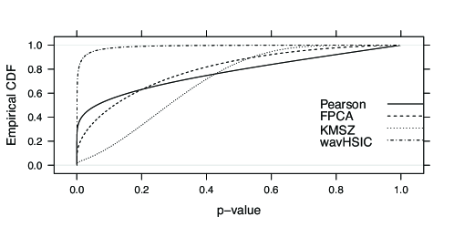
Figure 1: Empirical cumulative distribution function for the p-values for testing the independence between every pair of the 8,004 signals for each method.

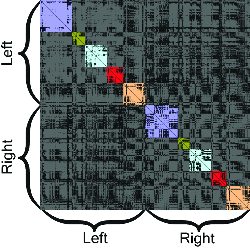
(a) Pearson

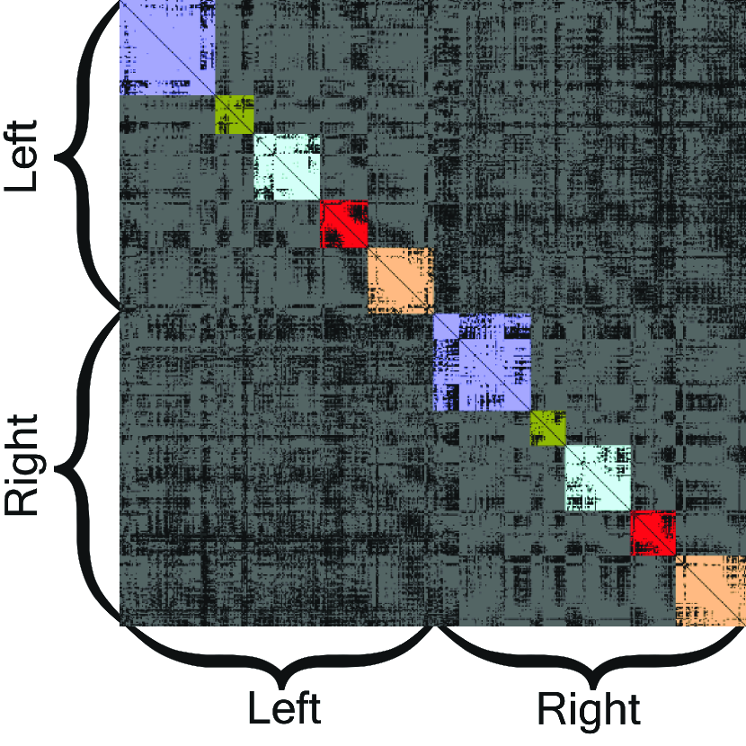
(b) FPCA

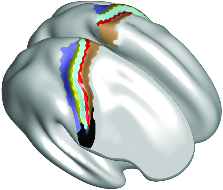
(c) Brain Cortex

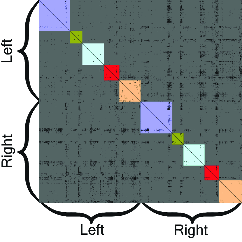
(d) KMSZ

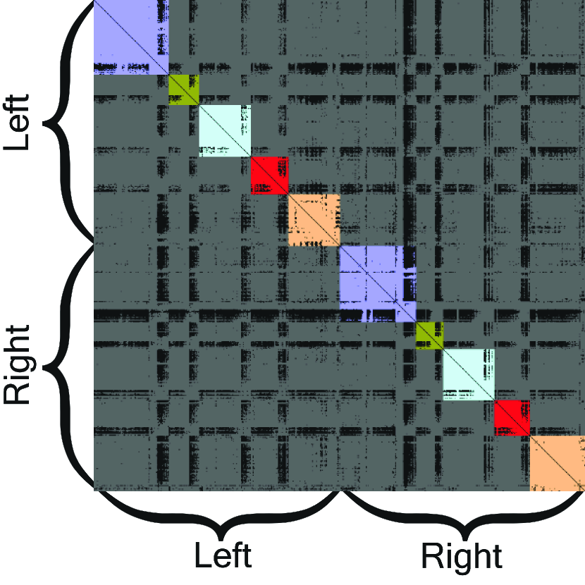
(e) wavHSIC

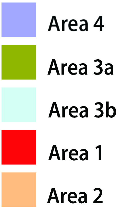
(f) Label

Figure 2: Functional connectivity networks of the five sensorimotor areas in the left and right hemispheres. In the adjacency matrices in (a), (b), (d) and (d) obtained by the four methods respectively, a bright entry indicates significant dependency between the corresponding signal pairs while a dark one indicates otherwise. The black subregion in (c) corresponds to face and eye portions and the rest of the colored area corresponds to upper limbs, trunk and lower limbs portions.

Appendix A Appendix: Background Materials

A.1 Distance-Induced Characteristic Kernels

Characteristic kernels are required to construct HSIC for two random functions under the RKHS framework. Such a kernel can be generated by a semi-metric of strong negative type.

Definition S3 (Strong Negative Type Semi-Metric).

A semi-metric $\rho:{\mathcal{Z}}\times{\mathcal{Z}}\rightarrow[0,\infty)$ defined on a non-empty set ${\mathcal{Z}}$ is of negative type if $\sum_{i=1}^{n}\sum_{j=1}^{n}\alpha_{i}\alpha_{j}\rho(z_{i},z_{j})\leq 0$ for all $z_{1},\dots,z_{n}\in{\mathcal{Z}}$ and $\alpha_{1},\dots,\alpha_{n}\in{\mathbb{R}}$ such that $\sum_{i=1}^{n}\alpha_{i}=0$, $n\geq 2$. Furthermore, it is of strong negative type if for any two probability measures $P$ and $P^{\prime}$ on ${\mathcal{Z}}$ such that $\int_{{\mathcal{Z}}}\rho(z,z_{0})dP(z),\int_{{\mathcal{Z}}}\rho(z,z_{0})dP^{\prime}(z)<\infty$ for some $z_{0}\in{\mathcal{Z}}$, we have $\int\rho\,d\{(P-P^{\prime})\times(P-P^{\prime})\}=0$ if and only if $P=P^{\prime}$.

Proposition S1 shows that a kernel induced by a strong negative type semi-metric is characteristic.

Proposition S1.

Let $\rho$ be a semi-metric defined on ${\mathcal{Z}}$ and $z_{0}\in{\mathcal{Z}}$. The induced kernel $\kappa_{\rho}\left(z,z^{\prime}\right)=\rho(z,z_{0})+\rho\left(z^{\prime},z_{0}\right)-\rho\left(z,z^{\prime}\right)$, $z,z^{\prime}\in{\mathcal{Z}}$, is symmetric and positive definite. Moreover, $\kappa_{\rho}$ is characteristic if and only if $\rho$ is of strong negative type.

Obviously distance-induced kernels are symmetric. For the proof of Proposition S1, see Lemma 2.1 of Berg et al. (1984) for positive definiteness and Lyons (2013) and Sejdinovic et al. (2013) for the characteristic property. Since the set ${\mathcal{Z}}$ of interest often contains zero, in this paper we always set $z_{0}=0$ for any distance-induced kernel $\kappa_{\rho}$ for simplicity and convenience.

A.2 Besov Spaces and Norms

The Besov space is a generalization of the Sobolev space, which is widely used in nonparametric regression under the RKHS framework. A Besov space $B_{p,q}^{\alpha}[0,1],p,q,\alpha>0,$ contains all functions of which Besov norm $\|\cdot\|_{B_{p,q}^{\alpha}}$ is finite. Explicitly, with any integer $r\geq 1$, define the $r$th order difference of a function $f$ by

$$\Delta_{h}^{r}(f,x)=\sum_{k=0}^{r}\binom{r}{k}(-1)^{r-k}f(x+kh),$$

and its $r$th order modulus of continuity by

$$\omega_{r}(f,t)_{p}=\sup_{0\leq h\leq t}\|\Delta_{h}^{r}(f,\cdot)\mid_{[0,1-rh]}\|_{L^{p}},$$

where $\Delta_{h}^{r}(f,\cdot)\mid_{[0,1-rh]}$ represents $\Delta_{h}^{r}(f,\cdot)$ restricted on $[0,1-rh]$ and $\|\cdot\|_{L^{p}}$ is the $L^{p}$ norm. Then the Besov norm of $f$ is defined by

$$\|f\|_{B_{p,q}^{\alpha}}=\|f\|_{L^{p}}+\left|f\right|_{B_{p,q}^{\alpha}},\quad\text{where}\quad\left|f\right|_{B_{p,q}^{\alpha}}=\left[\int_{0}^{\infty}\left\{\frac{\omega_{r}(f,t)_{p}}{t^{\alpha}}\right\}^{q}\frac{dt}{t}\right]^{\frac{1}{q}}.$$

For the same $\alpha$, the Besov norms generated by different values of $r>\alpha$ are equivalent when $p>1$ (DeVore and Lorentz, 1993). In this paper we always assume $p>1$ and $r=\lfloor\alpha\rfloor+1$ where $\lfloor\alpha\rfloor$ is the greatest integer less than or equal to $\alpha$.

The Besov norm (semi-norm) generalizes some traditional smoothness measures, such as the Sobolev semi-norm $|\cdot|_{W_{p}^{k}}$

$$|f|_{W_{p}^{k}}=\left(\int_{0}^{1}\left|D^{k}f\right|^{p}dx\right)^{1/p},~{}~{}1\leq p\leq\infty,$$

where $D^{k}$ is $k$th order weak-derivative operator.

Appendix B Appendix: Technical Proofs

B.1 Proof of Theorem 1

We first list two lemmas on some properties of negative type semi-metrics, which will be needed in the proof of Theorem 1.

Definition S4 (Radial Positive Definite Function).

A real function $F$ defined on ${\mathbb{R}}^{+}$ is called radial positive definite on the semi-metric space $({\mathcal{Z}},\rho)$ if $F$ is continuous and

$$\sum_{j=1}^{n}\sum_{k=1}^{n}F(\rho(z_{j},z_{k}))c_{j}c_{k}\geq 0,$$

for all choices of $n\geq 1$ points $z_{1},\dots,z_{n}\in{\mathcal{Z}}$. We denote the set of all radial positive definite functions by $\mbox{{\rm RPD}}({\mathcal{Z}})$.

Lemma S2.

The following hold in any semi-metric space ${\mathcal{Z}}$.

1. $\mbox{{\rm RPD}}({\mathcal{Z}})$ is never empty.

2. If $F_{1},F_{2}\in\mbox{{\rm RPD}}({\mathcal{Z}})$, then $F_{1}\cdot F_{2}\in\mbox{{\rm RPD}}({\mathcal{Z}})$.

3. If $F_{j}\in\mbox{{\rm RPD}}({\mathcal{Z}})$ and $0\leq c_{j}<\infty$, $j=1,\dots,n$, then $\sum_{j=1}^{n}c_{j}F_{j}\in\mbox{{\rm RPD}}({\mathcal{Z}})$.

4. If $F_{j}\in\mbox{{\rm RPD}}({\mathcal{Z}}),j=1,2,\dots$ and the $F_{j}$ converge point-wise to a continuous limit $F$, then $F\in\mbox{{\rm RPD}}({\mathcal{Z}})$

5. For space $(L^{p},\|\cdot\|_{p})$, $(\ell^{p},\|\cdot\|_{p})$ with $0<p\leq 2$, then $\exp(-t^{\alpha})$ is RPD for $0<\alpha\leq p$.

Lemma S2 is a combination of Theorems 4.4 and 4.10 of Wells and Williams (2012).

Lemma S3 (Theorem 4.5, Wells and Williams (2012)).

In a semi-metric space $({\mathcal{Z}},\rho)$, the following are equivalent:

1. $\rho$ is of negative type;

2. the function $\exp(-\lambda t)$ belongs to $\mbox{{\rm RPD}}({\mathcal{Z}},\rho)$ for $\lambda>0$;

3. $({\mathcal{Z}},\rho)$ is embeddable in a Hilbert space.

Proof of Theorem 1.

By Proposition S1, it suffices to prove that $\rho_{b^{\alpha}_{p,q}}$ is of strong negative type. Lemmas S2 (e) and S3 (a) ensure that $\bar{\rho}_{j}(f,g):=\|\mbox{\boldmath$\theta$}_{j}^{f}-\mbox{\boldmath$\theta$}_{j}^{g}\|_{p}^{q},j=-1,0,1,\dots$ are of negative type for $q\leq p\leq 2$.

By Lemma S3, the function $F_{j}(t)=\exp(-2^{sjq}t)$ belongs to $\mbox{{\rm RPD}}({\mathcal{Z}},\bar{\rho}_{j})$. For any finite product, by Lemma S2 (b)

$$\prod_{j=-1}^{n}F_{j}(\bar{\rho}_{j})=\exp\left\{-\sum_{j=-1}^{n}2^{sjq}\bar{\rho}_{j}\right\}$$ (3)

belongs to $\mbox{{\rm RPD}}({\mathcal{Z}})$. Lemma S2 (c) ensures the continuous sequence limit of (3), i.e., $\exp(-\rho_{b^{\alpha}_{p,q}})\in\mbox{{\rm RPD}}({\mathcal{Z}})$ as $n\rightarrow\infty$. Therefore $\rho_{b^{\alpha}_{p,q}}$ is of negative type on ${\mathcal{Z}}$. The separability of $B_{p,q}^{\alpha}[0,1]$ ensures that $\rho_{b^{\alpha}_{p,q}}$ is of strong negative type. ∎

B.2 Proof of Theorem 2

We first present a lemma that will be used to prove Theorem 2.

Lemma S4.

Let $\left\{(X_{i}(\cdot),Y_{i}(\cdot)\right\}_{i=1}^{n}$ be i.i.d. fully observed random samples from probability measure $P_{XY}=P_{X}P_{Y}$ defined on ${\mathcal{X}}\otimes{\mathcal{Y}}$. Then as $n\rightarrow\infty$,

$$n\gamma(P_{n,XY},\kappa_{\mathcal{X}},\kappa_{\mathcal{Y}})\rightsquigarrow\sum_{r=1}^{\infty}\sum_{s=1}^{\infty}\mu_{r}\nu_{s}N_{rs}^{2},$$ (4)

where $N_{rs}\sim N(0,1),r,s\in{\mathbb{N}}$ are i.i.d. and $\left\{\mu_{r}\right\}_{r=1}^{\infty}$ and $\left\{\nu_{s}\right\}_{s=1}^{\infty}$ are eigenvalues of the integral kernel operators $S_{{\check{\kappa}_{\mathcal{X}}}}$ and $S_{{\check{\kappa}_{\mathcal{Y}}}}$, respectively. If $P_{XY}\neq P_{X}P_{Y}$, then $n\gamma(P_{n,XY},\kappa_{\mathcal{X}},\kappa_{\mathcal{Y}})\rightarrow\infty$ in probability as $n\rightarrow\infty$.

Lemma S4 is exactly Theorem 33 of (Sejdinovic et al., 2013), which provides the weak convergence result of HSIC for fully observed random functions.

Proof of Theorem 2.

According to Lemma S4, it suffices to prove that the difference between HSIC based on original curves $\{X_{i}(\cdot),Y_{i}(\cdot)\}_{i=1}^{n}$ and HSIC based on denoised curves $\{{\hat{X}}_{i},{\hat{Y}}_{i}\}_{i=1}^{n}$ is $o_{p}(1/n)$, where $\{{\hat{X}}_{i},{\hat{Y}}_{i}\}_{i=1}^{n}$ are obtained by Step 1 in Section 3. By Definition 1,

$$n\left|\gamma(P_{n,XY},\kappa_{\mathcal{X}},\kappa_{\mathcal{Y}})-\gamma(P_{n,{\hat{X}}{\hat{Y}}},\kappa_{\mathcal{X}},\kappa_{\mathcal{Y}})\right|=n^{-1}\left|\|{\bm{\kappa}}_{\mathcal{X}}^{\top}{\bf H}{\bm{\kappa}}_{\mathcal{Y}}\|_{{{\mathcal{H}}(\kappa_{\mathcal{X}}\otimes\kappa_{\mathcal{Y}})}}^{2}-\|{\hat{\bm{\kappa}}_{\mathcal{X}}}^{\top}{\bf H}{\hat{\bm{\kappa}}_{\mathcal{Y}}}\|_{{{\mathcal{H}}(\kappa_{\mathcal{X}}\otimes\kappa_{\mathcal{Y}})}}^{2}\right|$$

$$= n^{-1}\left|\|{\bm{\kappa}}_{\mathcal{X}}^{\top}{\bf H}{\bm{\kappa}}_{\mathcal{Y}}\|_{{{\mathcal{H}}(\kappa_{\mathcal{X}}\otimes\kappa_{\mathcal{Y}})}}-\|{\hat{\bm{\kappa}}_{\mathcal{X}}}^{\top}{\bf H}{\hat{\bm{\kappa}}_{\mathcal{Y}}}\|_{{{\mathcal{H}}(\kappa_{\mathcal{X}}\otimes\kappa_{\mathcal{Y}})}}\right|\left(\|{\bm{\kappa}}_{\mathcal{X}}^{\top}{\bf H}{\bm{\kappa}}_{\mathcal{Y}}\|_{{{\mathcal{H}}(\kappa_{\mathcal{X}}\otimes\kappa_{\mathcal{Y}})}}+\|{\hat{\bm{\kappa}}_{\mathcal{X}}}^{\top}{\bf H}{\hat{\bm{\kappa}}_{\mathcal{Y}}}\|_{{{\mathcal{H}}(\kappa_{\mathcal{X}}\otimes\kappa_{\mathcal{Y}})}}\right)$$

$$\leq n^{-1}\|{\bm{\kappa}}_{\mathcal{X}}^{\top}{\bf H}{\bm{\kappa}}_{\mathcal{Y}}-{\hat{\bm{\kappa}}_{\mathcal{X}}}^{\top}{\bf H}{\hat{\bm{\kappa}}_{\mathcal{Y}}}\|_{{{\mathcal{H}}(\kappa_{\mathcal{X}}\otimes\kappa_{\mathcal{Y}})}}\left(\|{\bm{\kappa}}_{\mathcal{X}}^{\top}{\bf H}{\bm{\kappa}}_{\mathcal{Y}}\|_{{{\mathcal{H}}(\kappa_{\mathcal{X}}\otimes\kappa_{\mathcal{Y}})}}+\|{\hat{\bm{\kappa}}_{\mathcal{X}}}^{\top}{\bf H}{\hat{\bm{\kappa}}_{\mathcal{Y}}}\|_{{{\mathcal{H}}(\kappa_{\mathcal{X}}\otimes\kappa_{\mathcal{Y}})}}\right)$$

$$\leq 2n^{-1/2}\|{\bm{\kappa}}_{\mathcal{X}}^{\top}{\bf H}{\bm{\kappa}}_{\mathcal{Y}}-{\hat{\bm{\kappa}}_{\mathcal{X}}}^{\top}{\bf H}{\hat{\bm{\kappa}}_{\mathcal{Y}}}\|_{{{\mathcal{H}}(\kappa_{\mathcal{X}}\otimes\kappa_{\mathcal{Y}})}}\times n^{-1/2}\|{\bm{\kappa}}_{\mathcal{X}}^{\top}{\bf H}{\bm{\kappa}}_{\mathcal{Y}}\|_{{{\mathcal{H}}(\kappa_{\mathcal{X}}\otimes\kappa_{\mathcal{Y}})}}+n^{-1}\|{\bm{\kappa}}_{\mathcal{X}}^{\top}{\bf H}{\bm{\kappa}}_{\mathcal{Y}}-{\hat{\bm{\kappa}}_{\mathcal{X}}}^{\top}{\bf H}{\hat{\bm{\kappa}}_{\mathcal{Y}}}\|_{{{\mathcal{H}}(\kappa_{\mathcal{X}}\otimes\kappa_{\mathcal{Y}})}}^{2}$$

where ${\bm{\kappa}}_{\mathcal{X}}^{\top}=\left[\kappa_{\mathcal{X}}(\cdot,X_{1}),\dots,\kappa_{\mathcal{X}}(\cdot,X_{n})\right]$, ${\bm{\kappa}}_{\mathcal{Y}}^{\top}=\left[\kappa_{\mathcal{Y}}(\cdot,Y_{1}),\dots,\kappa_{\mathcal{Y}}(\cdot,Y_{n})\right]$, ${\hat{\bm{\kappa}}_{\mathcal{X}}}^{\top}=\left[\kappa_{\mathcal{X}}(\cdot,{\hat{X}}_{1}),\dots,\kappa_{\mathcal{X}}(\cdot,{\hat{X}}_{n})\right]$, ${\hat{\bm{\kappa}}_{\mathcal{Y}}}^{\top}=\left[\kappa_{\mathcal{Y}}(\cdot,{\hat{Y}}_{1}),\dots,\kappa_{\mathcal{Y}}(\cdot,{\hat{Y}}_{n})\right]$.

By (4),

$$n^{-1/2}\|{\bm{\kappa}}_{\mathcal{X}}^{\top}{\bf H}{\bm{\kappa}}_{\mathcal{Y}}\|_{{{\mathcal{H}}(\kappa_{\mathcal{X}}\otimes\kappa_{\mathcal{Y}})}}\rightsquigarrow\sqrt{\sum_{r=1}^{\infty}\sum_{s=1}^{\infty}\mu_{r}\nu_{s}N_{rs}^{2}}=O_{p}(1),$$ (5)

so it suffices to prove that $\|{\bm{\kappa}}_{\mathcal{X}}^{\top}{\bf H}{\bm{\kappa}}_{\mathcal{Y}}-{\hat{\bm{\kappa}}_{\mathcal{X}}}^{\top}{\bf H}{\hat{\bm{\kappa}}_{\mathcal{Y}}}\|_{{{\mathcal{H}}(\kappa_{\mathcal{X}}\otimes\kappa_{\mathcal{Y}})}}=o_{p}\left(n^{1/2}\right).$

Notice that $\|{\bm{\kappa}}_{\mathcal{X}}^{\top}{\bf H}{\bm{\kappa}}_{\mathcal{Y}}-{\hat{\bm{\kappa}}_{\mathcal{X}}}^{\top}{\bf H}{\hat{\bm{\kappa}}_{\mathcal{Y}}}\|_{{{\mathcal{H}}(\kappa_{\mathcal{X}}\otimes\kappa_{\mathcal{Y}})}}$ can be bounded by the following inequality:

$$\quad\|{\bm{\kappa}}_{\mathcal{X}}^{\top}{\bf H}{\bm{\kappa}}_{\mathcal{Y}}-{\hat{\bm{\kappa}}_{\mathcal{X}}}^{\top}{\bf H}{\hat{\bm{\kappa}}_{\mathcal{Y}}}\|_{{{\mathcal{H}}(\kappa_{\mathcal{X}}\otimes\kappa_{\mathcal{Y}})}}=\|{\bm{\kappa}}_{\mathcal{X}}^{\top}{\bf H}\left({\bm{\kappa}}_{\mathcal{Y}}-{\hat{\bm{\kappa}}_{\mathcal{Y}}}\right)+\left({\bm{\kappa}}_{\mathcal{X}}-{\hat{\bm{\kappa}}_{\mathcal{X}}}\right){\bf H}{\hat{\bm{\kappa}}_{\mathcal{Y}}}^{\top}\|_{{{\mathcal{H}}(\kappa_{\mathcal{X}}\otimes\kappa_{\mathcal{Y}})}}$$

$$\leq\|{\bm{\kappa}}_{\mathcal{X}}^{\top}{\bf H}\left({\bm{\kappa}}_{\mathcal{Y}}-{\hat{\bm{\kappa}}_{\mathcal{Y}}}\right)\|_{{{\mathcal{H}}(\kappa_{\mathcal{X}}\otimes\kappa_{\mathcal{Y}})}}+\|\left({\bm{\kappa}}_{\mathcal{X}}-{\hat{\bm{\kappa}}_{\mathcal{X}}}\right){\bf H}{\hat{\bm{\kappa}}_{\mathcal{Y}}}^{\top}\|_{{{\mathcal{H}}(\kappa_{\mathcal{X}}\otimes\kappa_{\mathcal{Y}})}}$$

$$\leq\|{\bm{\kappa}}_{\mathcal{X}}^{\top}{\bf H}\left({\bm{\kappa}}_{\mathcal{Y}}-{\hat{\bm{\kappa}}_{\mathcal{Y}}}\right)\|_{{{\mathcal{H}}(\kappa_{\mathcal{X}}\otimes\kappa_{\mathcal{Y}})}}+\|\left({\bm{\kappa}}_{\mathcal{X}}-{\hat{\bm{\kappa}}_{\mathcal{X}}}\right){\bf H}{\bm{\kappa}}_{\mathcal{Y}}^{\top}\|_{{{\mathcal{H}}(\kappa_{\mathcal{X}}\otimes\kappa_{\mathcal{Y}})}}+\|\left({\bm{\kappa}}_{\mathcal{X}}-{\hat{\bm{\kappa}}_{\mathcal{X}}}\right){\bf H}\left({\bm{\kappa}}_{\mathcal{Y}}-{\hat{\bm{\kappa}}_{\mathcal{Y}}}\right)^{\top}\|_{{{\mathcal{H}}(\kappa_{\mathcal{X}}\otimes\kappa_{\mathcal{Y}})}}$$

$$=\mbox{{\rm tr}}^{\frac{1}{2}}\left({\bm{\Gamma}^{X}}{\bf H}\langle{\bm{\kappa}}_{\mathcal{Y}}-{\hat{\bm{\kappa}}_{\mathcal{Y}}},{\bm{\kappa}}_{\mathcal{Y}}^{\top}-{\hat{\bm{\kappa}}_{\mathcal{Y}}}^{\top}\rangle_{{{\mathcal{H}}(\kappa_{\mathcal{Y}})}}{\bf H}\right)+\mbox{{\rm tr}}^{\frac{1}{2}}\left({\bm{\Gamma}^{Y}}{\bf H}\langle{\bm{\kappa}}_{\mathcal{X}}-{\hat{\bm{\kappa}}_{\mathcal{X}}},{\bm{\kappa}}_{\mathcal{X}}^{\top}-{\hat{\bm{\kappa}}_{\mathcal{X}}}^{\top}\rangle_{{{\mathcal{H}}(\kappa_{\mathcal{X}})}}{\bf H}\right)$$

$$\quad+\mbox{{\rm tr}}^{\frac{1}{2}}\left(\langle{\bm{\kappa}}_{\mathcal{X}}-{\hat{\bm{\kappa}}_{\mathcal{X}}},{\bm{\kappa}}_{\mathcal{X}}^{\top}-{\hat{\bm{\kappa}}_{\mathcal{X}}}^{\top}\rangle_{{{\mathcal{H}}(\kappa_{\mathcal{X}})}}{\bf H}\langle{\bm{\kappa}}_{\mathcal{Y}}-{\hat{\bm{\kappa}}_{\mathcal{Y}}},{\bm{\kappa}}_{\mathcal{Y}}^{\top}-{\hat{\bm{\kappa}}_{\mathcal{Y}}}^{\top}\rangle_{{{\mathcal{H}}(\kappa_{\mathcal{Y}})}}{\bf H}\right)$$

$$=\mbox{{\rm tr}}^{\frac{1}{2}}\left(\check{\bm{\Gamma}}^{X}\langle{\bm{\kappa}}_{\mathcal{Y}}-{\hat{\bm{\kappa}}_{\mathcal{Y}}},{\bm{\kappa}}_{\mathcal{Y}}^{\top}-{\hat{\bm{\kappa}}_{\mathcal{Y}}}^{\top}\rangle_{{{\mathcal{H}}(\kappa_{\mathcal{Y}})}}\right)+\mbox{{\rm tr}}^{\frac{1}{2}}\left(\check{\bm{\Gamma}}^{Y}\langle{\bm{\kappa}}_{\mathcal{X}}-{\hat{\bm{\kappa}}_{\mathcal{X}}},{\bm{\kappa}}_{\mathcal{X}}^{\top}-{\hat{\bm{\kappa}}_{\mathcal{X}}}^{\top}\rangle_{{{\mathcal{H}}(\kappa_{\mathcal{X}})}}\right)$$

$$\quad+\mbox{{\rm tr}}^{\frac{1}{2}}\left(\langle{\bm{\kappa}}_{\mathcal{X}}-{\hat{\bm{\kappa}}_{\mathcal{X}}},{\bm{\kappa}}_{\mathcal{X}}^{\top}-{\hat{\bm{\kappa}}_{\mathcal{X}}}^{\top}\rangle_{{{\mathcal{H}}(\kappa_{\mathcal{X}})}}{\bf H}\langle{\bm{\kappa}}_{\mathcal{Y}}-{\hat{\bm{\kappa}}_{\mathcal{Y}}},{\bm{\kappa}}_{\mathcal{Y}}^{\top}-{\hat{\bm{\kappa}}_{\mathcal{Y}}}^{\top}\rangle_{{{\mathcal{H}}(\kappa_{\mathcal{Y}})}}{\bf H}\right)$$

$$\leq\mbox{{\rm tr}}^{\frac{1}{2}}(\check{\bm{\Gamma}}^{X})\mbox{{\rm tr}}^{\frac{1}{2}}(\langle{\bm{\kappa}}_{\mathcal{Y}}-{\hat{\bm{\kappa}}_{\mathcal{Y}}},{\bm{\kappa}}_{\mathcal{Y}}^{\top}-{\hat{\bm{\kappa}}_{\mathcal{Y}}}^{\top}\rangle_{{{\mathcal{H}}(\kappa_{\mathcal{Y}})}})+\mbox{{\rm tr}}^{\frac{1}{2}}(\check{\bm{\Gamma}}^{Y})\mbox{{\rm tr}}^{\frac{1}{2}}(\langle{\bm{\kappa}}_{\mathcal{X}}-{\hat{\bm{\kappa}}_{\mathcal{X}}},{\bm{\kappa}}_{\mathcal{X}}^{\top}-{\hat{\bm{\kappa}}_{\mathcal{X}}}^{\top}\rangle_{{{\mathcal{H}}(\kappa_{\mathcal{X}})}})$$ (*)

$$\quad+\mbox{{\rm tr}}^{\frac{1}{2}}(\langle{\bm{\kappa}}_{\mathcal{X}}-{\hat{\bm{\kappa}}_{\mathcal{X}}},{\bm{\kappa}}_{\mathcal{X}}^{\top}-{\hat{\bm{\kappa}}_{\mathcal{X}}}^{\top}\rangle_{{{\mathcal{H}}(\kappa_{\mathcal{X}})}})\mbox{{\rm tr}}^{\frac{1}{2}}(\langle{\bm{\kappa}}_{\mathcal{Y}}-{\hat{\bm{\kappa}}_{\mathcal{Y}}},{\bm{\kappa}}_{\mathcal{Y}}^{\top}-{\hat{\bm{\kappa}}_{\mathcal{Y}}}^{\top}\rangle_{{{\mathcal{H}}(\kappa_{\mathcal{Y}})}})=o_{p}(n^{1/2}),$$

where $\check{\bm{\Gamma}}^{X}={\bf H}{\bm{\Gamma}^{X}}{\bf H}$ and $\check{\bm{\Gamma}}^{Y}={\bf H}{\bm{\Gamma}^{Y}}{\bf H}$ are centered Gram matrices.

In (* ‣ B.2) we used the fact that for symmetric positive definite matrices ${\bf A}$ and ${\bf B}$,

$$\mbox{{\rm tr}}{\bf A}{\bf B}=\mbox{{\rm vec}}({\bf A})^{\top}\mbox{{\rm vec}}({\bf B})\leq\|{\bf A}\|_{F}\|{\bf B}\|_{F}=\sqrt{\mbox{{\rm tr}}{\bf A}^{2}\mbox{{\rm tr}}{\bf B}^{2}}\leq\mbox{{\rm tr}}{\bf A}\mbox{{\rm tr}}{\bf B}.$$

The last equation holds due to the facts below with $({\mathcal{Z}},Z,z)=({\mathcal{X}},X,x)$ or $({\mathcal{Y}},Y,y)$:

• $\mbox{{\rm tr}}(\check{\bm{\Gamma}}^{Z})=O_{p}(n)$ because $\int_{{\mathcal{Z}}}{\check{\kappa}_{\mathcal{Z}}}(z,z)dP_{Z}<\infty$ which is ensured by the assumptions in Lemma 1.

• $\mbox{{\rm tr}}\langle{\bm{\kappa}}_{\mathcal{Z}}-{\hat{\bm{\kappa}}_{\mathcal{Z}}},{\bm{\kappa}}_{\mathcal{Z}}^{\top}-{\hat{\bm{\kappa}}_{\mathcal{Z}}}^{\top}\rangle_{{{\mathcal{H}}(\kappa_{\mathcal{Z}})}}=\sum_{i=1}^{n}\|\kappa_{\mathcal{Z}}(\cdot,Z_{i})-\kappa_{\mathcal{Z}}(\cdot,{\hat{Z}}_{i})\|_{{{\mathcal{H}}(\kappa_{\mathcal{Z}})}}^{2}=o_{p}(1)$, because

  $$\|\kappa_{\mathcal{Z}}(\cdot,Z_{i})-\kappa_{\mathcal{Z}}(\cdot,{\hat{Z}}_{i})\|_{{{\mathcal{H}}(\kappa_{\mathcal{Z}})}}^{2}=\kappa_{\mathcal{Z}}(Z_{i},Z_{i})+\kappa_{\mathcal{Z}}({\hat{Z}}_{i},{\hat{Z}}_{i})-2\kappa_{\mathcal{Z}}(Z_{i},{\hat{Z}}_{i})$$

  $$= 2\|Z_{i}\|_{b^{\beta_{Z}}}^{2}+2\|{\hat{Z}}_{i}\|_{b^{\beta_{Z}}}^{2}-2\left(\|Z_{i}\|_{b^{\beta_{Z}}}^{2}+\|{\hat{Z}}_{i}\|_{b^{\beta_{Z}}}^{2}-\|Z_{i}-{\hat{Z}}_{i}\|_{b^{\beta_{Z}}}^{2}\right)=2\|Z_{i}-{\hat{Z}}_{i}\|_{b^{\beta_{Z}}}^{2},$$

  and $\|Z_{i}-{\hat{Z}}_{i}\|_{b^{\beta_{Z}}}^{2}=o_{p}(n^{-1}),i=1,\dots,n$ ensured by Lemma 1.

∎

B.3 Proof of Theorem 3

We first introduce a few notations. To perform a permutation test, let ${\mathcal{S}}(n)=\{\sigma_{1},\dots,\sigma_{n!}\}$ be the cyclic group of $\{1,\dots,n\}$. For a permutation $\sigma$ randomly selected from ${\mathcal{S}}(n)$, let $\gamma(P_{n,{\hat{X}}{\hat{Y}}}^{\sigma},\kappa_{\mathcal{X}},\kappa_{\mathcal{Y}})=n^{-2}\mbox{{\rm tr}}({\bm{\Gamma}^{{\hat{X}}}}{\bf H}{\bm{\Gamma}^{{\hat{Y}}}}(\sigma){\bf H})$, where ${\bm{\Gamma}^{{\hat{Y}}}}(\sigma)$ is generated by ${\bm{\Gamma}^{{\hat{Y}}}}$ with rows and columns permuted according to $\sigma$. Let $R$ be the rank of $\gamma(P_{n,{\hat{X}}{\hat{Y}}},\kappa_{\mathcal{X}},\kappa_{\mathcal{Y}})$ in all possible permuted HSICs. Then we reject $H_{0}:P_{XY}=P_{X}P_{Y}$ if $p_{{\hat{X}}{\hat{Y}}}=R/n!\leq\alpha$, where $p_{{\hat{X}}{\hat{Y}}}$ denotes the p-value of the permutation test enumerating all permutations and $\alpha$ is the level of significance.

In practice, it is impractical to consider all permutations from ${\mathcal{S}}(n)$. Hence we use a Monte-Carlo approximation by randomly choosing $B$ permutations $\sigma_{1},\dots,\sigma_{B}\in{\mathcal{S}}(n)\backslash\{\text{\rm{id}}\}$ where id refers to no permutation and calculating $\gamma(P_{n,{\hat{X}}{\hat{Y}}},\kappa_{\mathcal{X}},\kappa_{\mathcal{Y}}),\gamma(P_{n,{\hat{X}}{\hat{Y}}}^{\sigma_{1}},\kappa_{\mathcal{X}},\kappa_{\mathcal{Y}}),\dots,\gamma(P_{n,{\hat{X}}{\hat{Y}}}^{\sigma_{B}},\kappa_{\mathcal{X}},\kappa_{\mathcal{Y}})$. With a notational abuse, let $R$ be the rank of $\gamma(P_{n,{\hat{X}}{\hat{Y}}},\kappa_{\mathcal{X}},\kappa_{\mathcal{Y}})$ and we reject $H_{0}$ if $\hat{p}_{{\hat{X}}{\hat{Y}}}=R/(B+1)\leq\alpha$, where $\hat{p}_{{\hat{X}}{\hat{Y}}}$ is the p-value of the permutation test enumerating a finite sample of size $B$ from ${\mathcal{S}}(n)$.

If the value of $\gamma(P_{n,{\hat{X}}{\hat{Y}}},\kappa_{\mathcal{X}},\kappa_{\mathcal{Y}})$ repeats in $\{\gamma(P_{n,{\hat{X}}{\hat{Y}}}^{\sigma_{1}},\kappa_{\mathcal{X}},\kappa_{\mathcal{Y}}),\dots,\gamma(P_{n,{\hat{X}}{\hat{Y}}}^{\sigma_{B}},\kappa_{\mathcal{X}},\kappa_{\mathcal{Y}})\}$ for several times with $B\leq n!$, the rank $R$ of $\gamma(P_{n,{\hat{X}}{\hat{Y}}},\kappa_{\mathcal{X}},\kappa_{\mathcal{Y}})$ is determined by the following two ways proposed by Rindt et al. (2020).

• Breaking ties at random: $R$ is distributed uniformly on ranks of $\gamma(P_{n,{\hat{X}}{\hat{Y}}}^{\sigma},\kappa_{\mathcal{X}},\kappa_{\mathcal{Y}})$ that have the same value of $\gamma(P_{n,{\hat{X}}{\hat{Y}}},\kappa_{\mathcal{X}},\kappa_{\mathcal{Y}})$;

• Breaking ties conservatively: $R$ is the largest among ranks of $\gamma(P_{n,{\hat{X}}{\hat{Y}}}^{\sigma},\kappa_{\mathcal{X}},\kappa_{\mathcal{Y}})$ that have the same value of $\gamma(P_{n,{\hat{X}}{\hat{Y}}},\kappa_{\mathcal{X}},\kappa_{\mathcal{Y}})$.

Next we list two lemmas which will be useful to prove Theorem 3.

Lemma S5.

For $\sigma$ randomly selected from ${\mathcal{S}}(n)$, $\gamma(P_{n,{\hat{X}}{\hat{Y}}},\kappa_{\mathcal{X}},\kappa_{\mathcal{Y}})\rightarrow 0$ in probability as $n\rightarrow\infty$.

Lemma S5 is a direct application of Theorem 3 of Rindt et al. (2020) for $d=2$.

Lemma S6.

Suppose that the alternative hypothesis $H_{1}:P_{XY}\neq P_{X}P_{Y}$ is true and noises are i.i.d. Let $\{t_{n}^{1}({\hat{\mathcal{D}}})\geq\dots\geq t_{n}^{n!}({\hat{\mathcal{D}}})\}$ be ordered values of HSIC computed on all permutations of denoised curves $\{\gamma(P_{n,{\hat{X}}{\hat{Y}}}^{\sigma_{1}},\kappa_{\mathcal{X}},\kappa_{\mathcal{Y}}),\dots,\gamma(P_{n,{\hat{X}}{\hat{Y}}}^{\sigma_{n!}},\kappa_{\mathcal{X}},\kappa_{\mathcal{Y}})\}$. Let $a=\lfloor n!\alpha\rfloor$ for any level of significance $\alpha\in(0,1)$. Then $t_{n}^{a}({\hat{\mathcal{D}}})\rightarrow 0$ in probability as $n\rightarrow\infty$.

Lemma S6 is a direct application of Theorem 4 of Rindt et al. (2020) for $d=2$.

Proof of Theorem 3.

Denote the fully observed dataset by ${\mathcal{D}}=\{(X_{i},Y_{i}):i=1,\dots,n\}$ and the denoised dataset by ${\hat{\mathcal{D}}}=\{({\hat{X}}_{i},{\hat{Y}}_{i}):i=1,\dots,n\}$. For a permutation $\sigma\in{\mathcal{S}}(n)$, denote the permuted datasets by $\sigma({\mathcal{D}})$ and $\sigma({\hat{\mathcal{D}}})$, resulting in permuted HSIC $\gamma(P_{n,XY}^{\sigma},\kappa_{\mathcal{X}},\kappa_{\mathcal{Y}})$ and $\gamma(P_{n,{\hat{X}}{\hat{Y}}}^{\sigma},\kappa_{\mathcal{X}},\kappa_{\mathcal{Y}})$ respectively.

If $H_{0}:P_{XY}=P_{X}P_{Y}$ is true, then for any $\sigma\in{\mathcal{S}}(n)$, ${\mathcal{D}}$ and $\sigma({\mathcal{D}})$ have the same distribution and ${\hat{\mathcal{D}}}$ and $\sigma({\hat{\mathcal{D}}})$ have the same distribution due to the facts that the noise across subjects are i.i.d and that the denoising procedure in Section 3 is separately for each subject. For $B$ permutations $\sigma_{1},\dots,\sigma_{B}$ randomly selected from ${\mathcal{S}}(n)\backslash\{\text{\rm{id}}\}$, $({\mathcal{D}},\sigma_{1}({\mathcal{D}}),\dots,\sigma_{B}({\mathcal{D}}))$ is an exchangeable vector, and thus $\left(\gamma(P_{n,{\hat{X}}{\hat{Y}}},\kappa_{\mathcal{X}},\kappa_{\mathcal{Y}}),\gamma(P_{n,{\hat{X}}{\hat{Y}}}^{\sigma_{1}},\kappa_{\mathcal{X}},\kappa_{\mathcal{Y}}),\dots,\gamma(P_{n,{\hat{X}}{\hat{Y}}}^{\sigma_{B}},\kappa_{\mathcal{X}},\kappa_{\mathcal{Y}})\right)$ is exchangeable.

By breaking ties at random, each entry is equally likely to have any given rank, so the rank of $\gamma(P_{n,{\hat{X}}{\hat{Y}}},\kappa_{\mathcal{X}},\kappa_{\mathcal{Y}})$ is uniformly distributed in $\{1,\dots,B\}$. Therefore the type I error rate can be controlled for any level of significance $\alpha\in(0,1)$. Breaking ties conservatively can result in an even smaller Type I error rate.

If $H_{1}:P_{XY}\neq P_{X}P_{Y}$ is true, then by the definition of $t_{n}^{a}({\hat{\mathcal{D}}})$ in Lemma S6, we reject $H_{0}:P_{XY}=P_{X}P_{Y}$ if $\gamma(P_{n,{\hat{X}}{\hat{Y}}},\kappa_{\mathcal{X}},\kappa_{\mathcal{Y}})>t_{n}^{a}({\hat{\mathcal{D}}})$. For any $\alpha\in(0,1)$,

$$\lim_{n\rightarrow\infty}P(p_{{\hat{X}}{\hat{Y}}}\leq\alpha)\geq\lim_{n\rightarrow\infty}P(\gamma(P_{n,{\hat{X}}{\hat{Y}}},\kappa_{\mathcal{X}},\kappa_{\mathcal{Y}})>t_{n}^{a}({\hat{\mathcal{D}}}))=1,$$

since $\gamma(P_{n,{\hat{X}}{\hat{Y}}},\kappa_{\mathcal{X}},\kappa_{\mathcal{Y}})\rightarrow\gamma(P_{XY},\kappa_{\mathcal{X}},\kappa_{\mathcal{Y}})>0$ in probability as $n\rightarrow\infty$ by the proof of Theorem 2.

For a finite number $B$ of permutations, the p-value $\hat{p}_{{\hat{X}}{\hat{Y}}}=(1+U)/(B+1)$ where $U\sim\text{Binomial}(B,p_{{\hat{X}}{\hat{Y}}})$. If $U=0$, then $\hat{p}_{{\hat{X}}{\hat{Y}}}=1/(B+1)\leq\alpha$ and we reject the null hypothesis. Since $P(p_{{\hat{X}}{\hat{Y}}}\leq{\epsilon}_{1})\geq 1-{\epsilon}_{2}$ for some ${\epsilon}_{1},{\epsilon}_{2}>0$. For $n$ large enough, we have

$$P(\hat{p}_{{\hat{X}}{\hat{Y}}}) \geq P(\hat{p}_{{\hat{X}}{\hat{Y}}}=1/(B+1)\mid p_{{\hat{X}}{\hat{Y}}}\leq{\epsilon}_{1})P(p_{{\hat{X}}{\hat{Y}}}\leq{\epsilon}_{1})$$

$$\geq(1-{\epsilon}_{1})^{B}(1-{\epsilon}_{2}).$$

Then the consistency of the permutation test is proved by letting ${\epsilon}_{1},{\epsilon}_{2}\rightarrow 0$. ∎

References

- Antoniadis and Sapatinas (2007) Antoniadis, A. and T. Sapatinas (2007). Estimation and inference in functional mixed-effects models. Computational Statistics & Data Analysis 51(10), 4793–4813.
- Berg et al. (1984) Berg, C., J. P. R. Christensen, and P. Ressel (1984). Harmonic analysis on semigroups: theory of positive definite and related functions, Volume 100. Springer.
- Cai and Brown (1999) Cai, T. T. and L. D. Brown (1999). Wavelet estimation for samples with random uniform design. Statistics & Probability Letters 42(3), 313–321.
- Chen et al. (2020) Chen, F., Q. Jiang, Z. Feng, and L. Zhu (2020). Model checks for functional linear regression models based on projected empirical processes. Computational Statistics & Data Analysis 144, 106897.
- Cohen et al. (1993) Cohen, A., I. Daubechies, B. Jawerth, and P. Vial (1993). Multiresolution analysis, wavelets and fast algorithms on an interval. Comptes rendus de l’Académie des sciences. Série 1, Mathématique 316(5), 417–421.
- Daubechies (1992) Daubechies, I. (1992). Ten lectures on wavelets, Volume 61. SIAM.
- DeVore and Lorentz (1993) DeVore, R. A. and G. G. Lorentz (1993). Constructive approximation, Volume 303. Springer-Verlag Berlin Heidelberg.
- Donoho et al. (1995) Donoho, D. L., I. M. Johnstone, G. Kerkyacharian, and D. Picard (1995). Wavelet shrinkage: asymptopia? Journal of the Royal Statistical Society: Series B (Methodological) 57(2), 301–337.
- Dubin and Müller (2005) Dubin, J. A. and H.-G. Müller (2005). Dynamical correlation for multivariate longitudinal data. Journal of the American Statistical Association 100(471), 872–881.
- Eubank and Hsing (2008) Eubank, R. L. and T. Hsing (2008). Canonical correlation for stochastic processes. Stochastic Processes and their Applications 118(9), 1634–1661.
- Ferraty and Vieu (2006) Ferraty, F. and P. Vieu (2006). Nonparametric functional data analysis: theory and practice. Springer, New York.
- Glasser et al. (2016) Glasser, M. F., T. S. Coalson, E. C. Robinson, C. D. Hacker, J. Harwell, E. Yacoub, K. Ugurbil, J. Andersson, C. F. Beckmann, M. Jenkinson, S. M. Smith, and D. C. Van Essen (2016, Aug). A multi-modal parcellation of human cerebral cortex. Nature 536(7615), 171–178.
- Gretton et al. (2005) Gretton, A., O. Bousquet, A. Smola, and B. Schölkopf (2005). Measuring statistical dependence with hilbert-schmidt norms. In International conference on algorithmic learning theory, pp. 63–77. Springer.
- Gretton et al. (2008) Gretton, A., K. Fukumizu, C. H. Teo, L. Song, B. Schölkopf, and A. J. Smola (2008). A kernel statistical test of independence. In Advances in neural information processing systems, pp. 585–592.
- Guo (2002) Guo, W. (2002). Functional mixed effects models. Biometrics 58(1), 121–128.
- He et al. (2003) He, G., H.-G. Müller, and J.-L. Wang (2003). Functional canonical analysis for square integrable stochastic processes. Journal of Multivariate Analysis 85(1), 54–77.
- He et al. (2012) He, J., O. Carmichael, E. Fletcher, B. Singh, A.-M. Iosif, O. Martinez, B. Reed, A. Yonelinas, and C. DeCarli (2012). Influence of functional connectivity and structural mri measures on episodic memory. Neurobiology of Aging 33(11), 2612–2620.
- Huang et al. (2002) Huang, J. Z., C. O. Wu, and L. Zhou (2002). Varying-coefficient models and basis function approximations for the analysis of repeated measurements. Biometrika 89(1), 111–128.
- Johnstone and Silverman (2005) Johnstone, I. M. and B. W. Silverman (2005). Empirical bayes selection of wavelet thresholds. Annals of Statistics 33(4), 1700–1752.
- Kokoszka et al. (2008) Kokoszka, P., I. Maslova, J. Sojka, and L. Zhu (2008). Testing for lack of dependence in the functional linear model. Canadian Journal of Statistics 36(2), 207–222.
- Kosorok (2009) Kosorok, M. R. (2009). Discussion of: Brownian distance covariance. Annals of Applied Statistics 3(4), 1270–1278.
- Kovac and Silverman (2000) Kovac, A. and B. W. Silverman (2000). Extending the scope of wavelet regression methods by coefficient-dependent thresholding. Journal of the American Statistical Association 95(449), 172–183.
- Lee et al. (2020) Lee, C., X. Zhang, and X. Shao (2020). Testing conditional mean independence for functional data. Biometrika, In press.
- Leurgans et al. (1993) Leurgans, S. E., R. A. Moyeed, and B. W. Silverman (1993). Canonical correlation analysis when the data are curves. Journal of the Royal Statistical Society. Series B (Methodological) 55(3), 725–740.
- Lyons (2013) Lyons, R. (2013). Distance covariance in metric spaces. The Annals of Probability 41(5), 3284–3305.
- Morettin et al. (2017) Morettin, P. A., A. Pinheiro, and B. Vidakovic (2017). Wavelets in functional data analysis. Springer.
- Morris (2015) Morris, J. S. (2015). Functional regression. Annual Review of Statistics and Its Application 2(1), 321–359.
- Ogden (1997) Ogden, R. T. (1997). Essential wavelets for statistical applications and data analysis. Springer Science & Business Media.
- Patilea et al. (2016) Patilea, V., C. Sánchez-Sellero, and M. Saumard (2016). Testing the predictor effect on a functional response. Journal of the American Statistical Association 111(516), 1684–1695.
- Pensky and Vidakovic (2001) Pensky, M. and B. Vidakovic (2001). On non-equally spaced wavelet regression. Annals of the Institute of Statistical Mathematics 53(4), 681–690.
- Ramsay and Silverman (2005) Ramsay, J. and B. Silverman (2005). Functional data analysis. Springer, New York.
- Rindt et al. (2020) Rindt, D., D. Sejdinovic, and D. Steinsaltz (2020). Consistency of permutation tests for hsic and dhsic. arXiv preprint arXiv:2005.06573.
- Sang et al. (2019) Sang, P., L. Wang, and J. Cao (2019). Weighted empirical likelihood inference for dynamical correlations. Computational Statistics & Data Analysis 131, 194–206.
- Sejdinovic et al. (2013) Sejdinovic, D., B. Sriperumbudur, A. Gretton, and K. Fukumizu (2013). Equivalence of distance-based and rkhs-based statistics in hypothesis testing. Annals of Statistics 41(5), 2263–2291.
- Shen and Faraway (2004) Shen, Q. and J. Faraway (2004). An f test for linear models with functional responses. Statistica Sinica 14, 1239–1257.
- Shin and Lee (2015) Shin, H. and S. Lee (2015). Canonical correlation analysis for irregularly and sparsely observed functional data. Journal of Multivariate Analysis 134, 1–18.
- Székely and Rizzo (2013) Székely, G. J. and M. L. Rizzo (2013). The distance correlation t-test of independence in high dimension. Journal of Multivariate Analysis 117, 193–213.
- Székely et al. (2007) Székely, G. J., M. L. Rizzo, and N. K. Bakirov (2007, 12). Measuring and testing dependence by correlation of distances. Annals of Statistics 35(6), 2769–2794.
- Tsai (2018) Tsai, S.-Y. (2018). Reproducibility of structural brain connectivity and network metrics using probabilistic diffusion tractography. Scientific Reports 8(1), 1–12.
- Van Wijk et al. (2010) Van Wijk, B. C., C. J. Stam, and A. Daffertshofer (2010). Comparing brain networks of different size and connectivity density using graph theory. PLOS ONE 5(10), e13701.
- Vidakovic (2009) Vidakovic, B. (2009). Statistical modeling by wavelets, Volume 503. John Wiley & Sons.
- Wells and Williams (2012) Wells, J. H. and L. R. Williams (2012). Embeddings and extensions in analysis, Volume 84. Springer Science & Business Media.
- Zhou et al. (2018) Zhou, Y., S.-C. Lin, and J.-L. Wang (2018). Local and global temporal correlations for longitudinal data. Journal of Multivariate Analysis 167, 1–14.