Generalized Score Matching for General Domains

Abstract

Estimation of density functions supported on general domains arises when the data is naturally restricted to a proper subset of the real space. This problem is complicated by typically intractable normalizing constants. Score matching provides a powerful tool for estimating densities with such intractable normalizing constants, but as originally proposed is limited to densities on $\mathbb{R}^{m}$ and $\mathbb{R}_{+}^{m}$. In this paper, we offer a natural generalization of score matching that accommodates densities supported on a very general class of domains. We apply the framework to truncated graphical and pairwise interaction models, and provide theoretical guarantees for the resulting estimators. We also generalize a recently proposed method from bounded to unbounded domains, and empirically demonstrate the advantages of our method.
KEY WORDS: Density estimation, graphical model, normalizing constant, sparsity, truncated distributions

1 Introduction

Probability density functions, especially in multivariate graphical models, are often defined only up to a normalizing constant. In higher dimensions, computation of the normalizing constant is typically an intractable problem that becomes worse when the distributions are defined only on a proper subset of the real space $\mathbb{R}^{m}$. For example, even truncated multivariate Gaussian densities have intractable normalizing constants except for special situations, e.g., with diagonal covariance matrices. This inability to calculate normalizing constants makes density estimation for general domains very challenging.

Score matching Hyvärinen (2005) is a computational efficient solution to density estimation that bypasses the calculation of normalizing constants and has enabled, in particular, large-scale applications of non-Gaussian graphical models Forbes and Lauritzen (2015); Lin et al. (2016); Yu et al. (2016); Sun et al. (2015); Yu et al. (2019a). Its original formulation targets distributions supported on $\mathbb{R}^{m}$. It was extended to treat the non-negative orthant $\mathbb{R}_{+}^{m}$ in (Hyvärinen, 2007), with more recent generalizations in Yu et al. (2018, 2019b). An extension to products of intervals like $[0,1]^{m}$ was given in (Janofsky, 2015, 2018; Tan et al., 2019), and more general bounded domains were considered in (Liu and Kanamori, 2019). Despite this progress, the existing approaches have important limitations: The method in Liu and Kanamori (2019) only allows for bounded support, and earlier methods for $\mathbb{R}_{+}^{m}$ and $[0,1]^{m}$ offer ad-hoc solutions that cannot be directly extended to more general domains. This paper addresses these limitations by developing a unifying framework that encompasses the existing methods and applies to unbounded domains. The framework enables new applications for more complicated domains yet retains the computational efficiency of the original score matching. The remainder of this introduction provides a more detailed review of the score matching estimator and the contributions of this paper.

1.1 Score Matching and its Generalizations

The original score matching estimator introduced in Hyvärinen (2005) is based on the idea of minimizing the Fisher distance given by the expected $\ell_{2}$ distance between the gradients of the true log density $\log p_{0}$ on $\mathbb{R}^{m}$ and a proposed log density $\log p$, that is,

$$\int_{\mathbb{R}^{m}}p_{0}(\bm{x})\|\nabla_{\bm{x}}\log p(\bm{x})-\nabla_{\bm{x}}\log p_{0}(\bm{x})\|_{2}^{2}\mathop{}\!\mathrm{d}\bm{x}.$$ (1)

Integration by parts leads to an associated empirical loss, in which an additive constant term depending only on $p_{0}$ is ignored. This loss avoids calculations of the normalizing constant through dealing with the derivatives of the log-densities only. Minimizing the empirical loss to derive an estimator is particularly convenient if $p$ belongs to an exponential family because the loss is then a quadratic function of the family’s canonical parameters. The latter property holds, in particular, for the Gaussian case, where the methods proposed by Liu and Luo (2015); Zhang and Zou (2014) constitute a special case of score matching.

In (Hyvärinen, 2007), the approach was generalized to densities on $\mathbb{R}_{+}^{m}=[0,\infty)^{m}$ by minimizing instead

$$\int_{\mathbb{R}_{+}^{m}}p_{0}(\bm{x})\|\nabla_{\bm{x}}\log p(\bm{x})\odot\bm{x}-\nabla_{\bm{x}}\log p_{0}(\bm{x})\odot\bm{x}\|_{2}^{2}\mathop{}\!\mathrm{d}\bm{x}.$$ (2)

The element-wise multiplication (“$\odot$”) with $\bm{x}$ dampens discontinuities at the boundary of $\mathbb{R}_{+}^{m}$ and facilitates integration by parts for deriving an empirical loss that does not depend on the true $p_{0}$.

In recent work, we proposed a generalized score matching approach for densities on $\mathbb{R}_{+}^{m}$ by using the square-root of slowly growing and preferably bounded functions $\bm{h}(\bm{x})$ in place of $\bm{x}$ in the element-wise multiplication (Yu et al., 2018, 2019b). This modification improves performance (theoretically and empirically) as it avoids higher moments in the empirical loss. Another recent work extended score matching to supports given by bounded open subsets $\mathfrak{D}\subset\mathbb{R}^{m}$ with piecewise smooth boundaries (Liu and Kanamori, 2019). The idea there is to minimize

$$\sup_{g\in\mathcal{G}}\int_{\mathfrak{D}}p_{0}(\bm{x})g(\bm{x})\|\nabla_{\bm{x}}\log p(\bm{x})-\nabla_{\bm{x}}\log p_{0}(\bm{x})\|_{2}^{2}\mathop{}\!\mathrm{d}\bm{x},$$ (3)

where $\mathcal{G}\equiv\{g|g(\bm{x})=0\,\forall\bm{x}\in\partial\mathfrak{D}\text{ and }g\text{ is 1-Lipschitz continuous}\}$, and $\partial\mathfrak{D}$ is the boundary of $\mathfrak{D}$. The supremum in the loss is achieved at $g_{0}(\bm{x})\equiv\min_{\bm{x}^{\prime}\in\partial\mathfrak{D}}\|\bm{x}-\bm{x}^{\prime}\|$, the distance of $\bm{x}$ to $\partial\mathfrak{D}$.

1.2 A Unifying Framework for General Domains

In this paper, we further extend generalized score matching with the aim of avoiding the limitations of existing work and allowing for general and possibly unbounded domains $\mathfrak{D}$ with positive Lebesgue measure. We require merely that all sections of $\mathfrak{D}\subseteq\mathbb{R}^{m}$, i.e., the sets of values of any component $x_{j}$ fixing all other components $\bm{x}_{-j}$, are countable disjoint unions of intervals in $\mathbb{R}$. This level of generality ought to cover all practical cases. To handle such domains, we compose the function $\bm{h}$ in the generalized score matching loss of Yu et al. (2018, 2019b) with a component-wise distance function $\bm{\varphi}=(\varphi_{1},\ldots,\varphi_{m}):\mathfrak{D}\to\mathbb{R}_{+}^{m}$. To define $\varphi_{j}(\bm{x})$, we consider the interval in the section given by $\bm{x}_{-j}$ that contains $x_{j}$ and compute the distance between $x_{j}$ and the boundary of this interval. The function $\varphi_{j}(\bm{x})$ is then defined as the minimum of the distance and a user-selected constant $C_{j}$. The loss resulting from this extension, with the composition $\bm{h}\circ\bm{\varphi}$ in place of $\bm{h}$, can again be approximated by an empirical loss that is quadratic in the canonical parameters of exponential families.

As an application of the proposed framework, we study a class of pairwise interaction models for an $m$-dimensional random vector $\bm{X}=(X_{i})_{i=1}^{m}$ that was considered in Yu et al. (2018, 2019b) and in special cases in earlier literature. These $a$-$b$ models postulate a probability density function proportional to

$$\exp\left\{-\frac{1}{2a}\bm{x}^{a}\mathbf{K}\bm{x}^{a}+\frac{1}{b}\bm{\eta}^{\top}\bm{x}^{b}\right\},\qquad\bm{x}\in\mathfrak{D}.$$ (4)

Where past work assumes $\mathfrak{D}=\mathbb{R}^{m}$ or $\mathfrak{D}=\mathbb{R}_{+}^{m}$, we here allow a general domain $\mathfrak{D}\subset\mathbb{R}^{m}$. In (4), $a\geq 0$ and $b\geq 0$ are known constants, and $\mathbf{K}\in\mathbb{R}^{m\times m}$ and $\bm{\eta}\in\mathbb{R}^{m}$ are unknown parameters to be estimated. For $a=0$ we define ${\bm{x}^{a}}^{\top}\mathbf{K}\bm{x}^{a}/a\equiv(\log\bm{x})^{\top}\mathbf{K}(\log\bm{x})$ and for $b=0$ we define $\bm{\eta}^{\top}\bm{x}^{b}/b\equiv\bm{\eta}^{\top}(\log\bm{x})$. The case where $a=0$ was not considered in Yu et al. (2018, 2019b). This model class provides a simple yet rich framework for pairwise interaction models. In particular, if $\mathfrak{D}=\mathfrak{D}_{1}\times\cdots\times\mathfrak{D}_{m}$ is a product set, then $X_{i}$ and $X_{j}$ are conditionally independent given all others if and only if $\kappa_{ij}=\kappa_{ji}=0$ in the interaction matrix $\mathbf{K}$; i.e., the $a$-$b$ models become graphical models (Maathuis et al., 2019). When $a=b=1$, model (4) is a (truncated) Gaussian graphical model, with $\bm{\Sigma}\equiv\mathbf{K}^{-1}$ the covariance matrix and $\bm{\Sigma}^{-1}\bm{\eta}$ the mean parameter. The case where $a=b=1/2$ with $\mathfrak{D}=\mathbb{R}_{+}^{m}$ is the exponential square root graphical model from Inouye et al. (2016).

For estimation of a sparse interaction matrix $\mathbf{K}$ in high-dimensional $a$-$b$ models, we take up an $\ell_{1}$ regularization approach considered in Lin et al. (2016) and improved in Yu et al. (2018, 2019b). In Yu et al. (2018, 2019b), we showed that this approach permits recovery of the support of $\mathbf{K}$ under sample complexity $n=\Omega(\log m)$ for Gaussians truncated to $\mathfrak{D}=\mathbb{R}_{+}^{m}$. Here, we prove that the same sample complexity is achieved for Gaussians truncated to any domain $\mathfrak{D}$ that is a finite disjoint union of convex sets with $n=\Omega(\log m)$ samples. In addition, we derive similar results for general $a$-$b$ models on bounded subsets of $\mathbb{R}_{+}^{m}$ with positive measure for $a>0$, or if $\log\mathfrak{D}$ is bounded for $a=0$. On unbounded domains for $a>0$ or for unbounded $\log\mathfrak{D}$ and $a=0$, we require $n$ to be $\Omega(\log m)$ times a factor that may weakly depend on $m$.

1.3 Organization of the Paper

The rest of the paper is structured as follows. We provide the necessary background on score matching in Section 2. In Section 3, we introduce and detail our new methodology, along with the regularized generalized estimator for exponential families. In Section 4, we define the $a$-$b$ interaction models and focus on application of our method to these models on domains with positive Lebesgue measure. Theoretical results and numerical experiments are given in Sections 5 and 6, respectively. We apply our method to a DNA methylation dataset in Section 7. Longer proofs are included in the Appendix. An implementation that incorporates various types of domain $\mathfrak{D}$ is available in the genscore R package.

1.4 Notation

We use lower-case letters for constant scalars, vectors and functions and upper-case letters for random scalars and vectors (except some special cases). We reserve regular font for scalars (e.g. $a$, $X$) and boldface for vectors (e.g. $\bm{a}$, $\bm{X}$), and $\mathbf{1}_{m}=(1,\dots,1)\in\mathbb{R}^{m}$. For two vectors $\bm{u},\bm{v}\in\mathbb{R}^{m}$, we write $\bm{u}\succ\bm{v}$ if $u_{j}>v_{j}$ for $j=1,\dots,m$. Matrices are in upright bold, with constant matrices in upper-case ($\mathbf{K}$, $\mathbf{M}$) and random data matrices in lower-case ($\mathbf{x}$, $\mathbf{y}$). Superscripts index rows and subscripts index columns in a data matrix $\mathbf{x}$, so, $\bm{X}^{(i)}$ is the $i$-th row, and $X_{j}^{(i)}$ is its $j$-th feature.

For vectors $\bm{u},\bm{v}\in\mathbb{R}^{m}$, $\bm{u}\odot\bm{v}\equiv(u_{1}v_{1},\ldots,u_{m}v_{m})$ denotes the Hadamard product (element-wise multiplication), and the $\ell_{a}$-norm for $a\geq 1$ is denoted $\|\bm{u}\|_{a}=(\sum_{j=1}^{m}|u_{j}|^{a})^{1/a}$, with $\|\bm{u}\|_{\infty}=\max_{j=1,\ldots,m}|u_{j}|$. For $a\in\mathbb{R}$, let $\bm{v}^{a}\equiv(v_{1}^{a},\ldots,v_{m}^{a})$. Similarly, for function $\bm{f}:\mathbb{R}^{m}\to\mathbb{R}^{m}$, $\bm{x}\mapsto(f_{1}(\bm{x}),\ldots,f_{m}(\bm{x}))$, we write $\bm{f}^{a}(\bm{x})\equiv(f_{1}^{a}(\bm{x}),\ldots,f_{m}^{a}(\bm{x}))$. Similarly, we also write $\bm{f}^{\prime}(\bm{x})\equiv(\partial f_{1}(\bm{x})/\partial x_{1},\ldots,\partial f_{m}(\bm{x})/\partial x_{m})$.

For a matrix $\mathbf{K}=[\kappa_{ij}]_{i,j}\in\mathbb{R}^{n\times m}$, its vectorization is obtained by stacking its columns into an $\mathbb{R}^{nm}$ vector. Its Frobenius norm is ${\left|\kern-1.07639pt\left|\kern-1.07639pt\left|\mathbf{K}\right|\kern-1.07639pt\right|\kern-1.07639pt\right|}_{F}=\|\mathrm{vec}(\mathbf{K})\|_{2}$, its max norm is $\|\mathbf{K}\|_{\infty}\equiv\|\mathrm{vec}(\mathbf{K})\|_{\infty}\equiv\max_{i,j}|\kappa_{ij}|$, and its $\ell_{a}$–$\ell_{b}$ operator norm is ${\left|\kern-1.07639pt\left|\kern-1.07639pt\left|\mathbf{K}\right|\kern-1.07639pt\right|\kern-1.07639pt\right|}_{a,b}\equiv\max_{\bm{x}\neq\bm{0}}\|\mathbf{K}\bm{x}\|_{b}/\|\bm{x}\|_{a}$, with ${\left|\kern-1.07639pt\left|\kern-1.07639pt\left|\mathbf{K}\right|\kern-1.07639pt\right|\kern-1.07639pt\right|}_{a}\equiv{\left|\kern-1.07639pt\left|\kern-1.07639pt\left|\mathbf{K}\right|\kern-1.07639pt\right|\kern-1.07639pt\right|}_{a,a}$.

For a vector $\bm{x}\in\mathbb{R}^{m}$ and an index $j\in\{1,\dots,m\}$, we write $\bm{x}_{-j}$ for the subvector that has the $j$th component removed. For a function $f$ of a vector $\bm{x}$, we may also write $f(x_{j};\bm{x}_{-j})$ to stress the dependency on $x_{j}$, especially when $\bm{x}_{-j}$ is fixed and only $x_{j}$ is varied, and write $\partial_{j}f(\bm{x})=\left.\partial_{j}f(y;\bm{x}_{-j})/\partial y\right|_{y\equiv x_{j}}$. For two compatible functions $f$ and $g$, $f\circ g$ denotes their function composition. Unless otherwise noted, the considered probability density functions are densities with respect to the Lebesgue measure on $\mathbb{R}^{m}$.

2 Preliminaries

Suppose $\bm{X}\in\mathbb{R}^{m}$ is a random vector with distribution function $P_{0}$ supported on domain $\mathfrak{D}\subseteq\mathbb{R}^{m}$ and a twice continuously differentiable probability density function $p_{0}$ with respect to the Lebesgue measure restricted to $\mathfrak{D}$. Let $\mathcal{P}(\mathfrak{D})$ be a family of distributions of interest with twice continuously differentiable densities on $\mathfrak{D}$. The goal is to estimate $p_{0}$ by picking the distribution $P$ from $\mathcal{P}(\mathfrak{D})$ with density $p$ minimizing an empirical loss that measures the distance between $p$ and $p_{0}$.

2.1 Original Score Matching on $\mathbb{R}^{m}$

The original score matching loss proposed by Hyvärinen (2005) for $\mathfrak{D}\equiv\mathbb{R}^{m}$ is given by

$$J_{\mathbb{R}^{m}}(P)\equiv\frac{1}{2}\int_{\mathbb{R}^{m}}p_{0}(\bm{x})\|\nabla\log p(\bm{x})-\nabla\log p_{0}(\bm{x})\|_{2}^{2}\mathop{}\!\mathrm{d}\bm{x},$$

in which the gradients can be thought of as gradients with respect to a hypothetical location parameter and evaluated at the origin (Hyvärinen, 2005). The log densities enable estimation without calculating the normalizing constants of $p$ and $p_{0}$. Under mild conditions, using integration by parts, the loss can be rewritten as

$$J_{\mathbb{R}^{m}}(P)\equiv\int_{\mathbb{R}^{m}}p_{0}(\bm{x})\sum_{j=1}^{m}\left[\partial_{jj}\log p(\bm{x})+\frac{1}{2}\left(\partial_{j}\log p(\bm{x})\right)^{2}\right]\mathop{}\!\mathrm{d}\bm{x}$$

plus a constant independent of $p$. One can thus use a sample average to approximate the loss without knowing the true density $p_{0}$.

2.2 Score Matching on $\mathbb{R}_{+}^{m}$

Consider $\mathfrak{D}\equiv\mathbb{R}_{+}^{m}$. Let $\bm{h}:\mathbb{R}_{+}^{m}\to\mathbb{R}_{+}^{m},\,\bm{x}\mapsto(h_{1}(x_{1}),\ldots,h_{m}(x_{m}))^{\top}$, where $h_{1},\ldots,h_{m}:\mathbb{R}_{+}\to\mathbb{R}_{+}$ are almost surely positive functions that are absolutely continuous in every bounded sub-interval of $\mathbb{R}_{+}$. The generalized $\bm{h}$-score matching loss proposed by Yu et al. (2018, 2019b) is

$$J_{\bm{h},\mathbb{R}_{+}^{m}}(P)\equiv\frac{1}{2}\int_{\mathbb{R}_{+}^{m}}p_{0}(\bm{x})\left\|\nabla\log p(\bm{x})\odot\bm{h}^{1/2}(\bm{x})-\nabla\log p_{0}(\bm{x})\odot\bm{h}^{1/2}(\bm{x})\right\|_{2}^{2}\mathop{}\!\mathrm{d}\bm{x}.$$ (5)

The score matching loss for $\mathbb{R}_{+}^{m}$ originally proposed by Hyvärinen (2007) is a special case of (5) with $\bm{h}(\bm{x})=\bm{x}^{2}$. In Yu et al. (2018, 2019b) we proved that by choosing slowly growing and preferably bounded $h_{1},\ldots,h_{m}$, the estimation efficiency can be significantly improved. Under assumptions that for all $P\in\mathcal{P}(\mathbb{R}_{+}^{m})$ with density $p$,

1. $p_{0}(x_{j};\bm{x}_{-j})h_{j}(x_{j})\partial_{j}\log p(x_{j};\bm{x}_{-j})\left|{}_{x_{j}\searrow 0^{+}}^{x_{j}\nearrow+\infty}\right.=0,\quad\forall\bm{x}_{-j}\in\mathbb{R}_{+}^{m-1}$ $\forall j$;

2. $\mathbb{E}_{p_{0}}\left\|\nabla\log p(\bm{X})\odot\bm{h}^{1/2}(\bm{X})\right\|_{2}^{2}<+\infty$, $\mathbb{E}_{p_{0}}\left\|\left(\nabla\log p(\bm{X})\odot\bm{h}(\bm{X})\right)^{\prime}\right\|_{1}<+\infty$,

where $f(\bm{x})\left|{}^{x_{j}\nearrow+\infty}_{x_{j}\searrow 0^{+}}\right.\equiv\lim_{x_{j}\nearrow+\infty}f(\bm{x})-\lim_{x_{j}\searrow 0^{+}}f(\bm{x})$, the loss (5) can be rewritten as

$$J_{\bm{h},\mathbb{R}_{+}^{m}}(P)\equiv\int_{\mathbb{R}_{+}^{m}}p_{0}(\bm{x})\sum_{j=1}^{m}\left[h_{j}^{\prime}(x_{j})\partial_{j}(\log p(\bm{x}))+h_{j}(x_{j})\partial_{jj}(\log p(\bm{x}))+\frac{1}{2}h_{j}(x_{j})[\partial_{j}(\log p(\bm{x}))]^{2}\right]\mathop{}\!\mathrm{d}\bm{x}$$

plus a constant independent of $p$. One can thus estimate $p_{0}$ by minimizing the empirical loss $J_{\bm{h},\mathbb{R}_{+}^{m}}(P)$.

2.3 Score Matching on Bounded Open Subsets of $\mathbb{R}^{m}$

The method proposed in Liu and Kanamori (2019) estimates a density $p_{0}$ on a bounded open subset $\mathfrak{D}\subset\mathbb{R}^{m}$ with a piecewise smooth boundary $\partial\mathfrak{D}$ by minimizing the following “maximally weighted score matching” loss

$$J_{g_{0},\mathfrak{D}}(P)\equiv\sup_{g\in\mathcal{G}}\frac{1}{2}\int_{\mathbb{R}_{+}^{m}}g(\bm{x})p_{0}(\bm{x})\left\|\nabla\log p(\bm{x})-\nabla\log p_{0}(\bm{x})\right\|_{2}^{2}\mathop{}\!\mathrm{d}\bm{x}.$$ (6)

with $\mathcal{G}\equiv\{g|g(\bm{x})=0,\forall\bm{x}\in\partial\mathfrak{D}\text{ and }g\text{ is }L\text{-Lipschitz continuous}\}$ for some constant $L>0$. The authors show that the maximum is obtained with $g_{0}(\bm{x})\equiv L\cdot\inf_{\bm{x}^{\prime}\in\partial\mathfrak{D}}\|\bm{x}-\bm{x}^{\prime}\|_{2}$, i.e. the $\ell_{2}$ distance of $\bm{x}$ to the boundary of $\mathfrak{D}$; using integration by parts similar to the previous methods, (6) can be estimated using the empirical loss which can be calculated with a closed form.

3 Generalized Score Matching for General Domains

3.1 Assumption on the Domain

For $\bm{x}\in\mathbb{R}^{m}$ and any index $j=1,\ldots,m$, write $\mathfrak{C}_{j,\mathfrak{D}}\left(\bm{x}_{-j}\right)\equiv\{y\in\mathbb{R}:(y;\bm{x}_{-j})\in\mathfrak{D}\}$ for the section of $\mathfrak{D}$ obtained by fixing the coordinates in $\bm{x}_{-j}$. This $j$th section is the projection of the intersection between $\mathfrak{D}$ and the line $\{(y;\bm{x}_{-j}):y\in\mathbb{R}\}$. A non-empty $j$th section is obtained from the vectors $\bm{x}_{-j}$ in the set $\mathfrak{S}_{-j,\mathfrak{D}}\equiv\left\{\bm{x}_{-j}:\mathfrak{C}_{j,\mathfrak{D}}\left(\bm{x}_{-j}\right)\neq\varnothing\right\}\subset\mathbb{R}^{m-1}$. For notational simplicity, we drop their dependency on $\mathfrak{D}$.

Definition 1.

We say that a domain $\mathfrak{D}\subseteq\mathbb{R}^{m}$ is a component-wise countable union of intervals if it is measurable, and for any index $j=1,\ldots,m$ and any $\bm{x}_{-j}\in\mathfrak{S}_{-j,\mathfrak{D}}$, the section $\mathfrak{C}_{j,\mathfrak{D}}\left(\bm{x}_{-j}\right)$ is a countable union of disjoint intervals, meaning that

$$\mathfrak{C}_{j,\mathfrak{D}}\left(\bm{x}_{-j}\right)\equiv\operatorname*{\cup}_{k=1}^{K_{j}(\bm{x}_{-j})}I_{k}(\bm{x}_{-j}),$$ (7)

where $K_{j}(\bm{x}_{-j})\in\mathbb{N}\cup\{\infty\}$, and each set $I_{k}(\bm{x}_{-j})$ is an interval (closed, open, or half-open) with endpoints $-\infty\leq a_{k,j}(\bm{x}_{-j})\leq b_{k,j}(\bm{x}_{-j})\leq+\infty$, with the $I_{k}(\bm{x}_{-j})$’s being the connected components of $\mathfrak{C}_{j,\mathfrak{D}}\left(\bm{x}_{-j}\right)$. The last point rules out constructions like $I_{1}=(0,1]$ and $I_{2}=(1,2]$ but allows $I_{1}=(0,1)$ and $I_{2}=(1,2]$. We define the component-wise boundary set of such a component-wise countable union of intervals as

$$\underline{\partial}\mathfrak{D}\equiv\left\{\bm{x}\in\mathbb{R}^{m}:\exists j=1,\ldots,m,\,\bm{x}_{-j}\in\mathfrak{S}_{-j,\mathfrak{D}},\,x_{j}\in\operatorname*{\cup}_{k=1}^{K_{j}(\bm{x}_{-j})}\{a_{k,j}(\bm{x}_{-j}),b_{k,j}(\bm{x}_{-j})\}\backslash\{\pm\infty\}\right\}.$$ (8)

3.2 Generalized Score Matching Loss for General Domains

We first define a truncated component-wise distance, which is based on distances within connected components of sections.

Definition 2.

Let $\bm{C}=(C_{1},\dots,C_{m})$ be comprised of positive constants, so $\bm{C}\succ\bm{0}$. Let $\mathfrak{D}\subseteq\mathbb{R}^{m}$ be a non-empty component-wise countable union of intervals whose sections are presented as in (7). For any vector $\bm{x}\in\mathfrak{D}$, define the truncated component-wise distance of $\bm{x}$ to the boundary of $\mathfrak{D}$ as

$$\bm{\varphi}_{\bm{C},\mathfrak{D}}(\bm{x}) \equiv\left(\varphi_{C_{1},\mathfrak{D},1}(\bm{x}),\ldots,\varphi_{C_{m},\mathfrak{D},m}(\bm{x})\right)\in\mathbb{R}_{+}^{m},$$ (9)

$$\varphi_{C_{j},\mathfrak{D},j}(\bm{x}) \equiv\begin{cases}C_{j},&a_{k,j}=-\infty,\,b_{k,j}=+\infty,\\ \min(C_{j},b_{k,j}-x_{j}),&a_{k,j}=-\infty,\,x_{j}\leq b_{k,j}<+\infty,\\ \min(C_{j},x_{j}-a_{k,j},b_{k,j}-x_{j}),&-\infty<a_{k,j}\leq x_{j}\leq b_{k,j}<+\infty,\\ \min(C_{j},x_{j}-a_{k,j}),&-\infty<a_{k,j}\leq x_{j},\,b_{k,j}=+\infty,\end{cases}$$ (10)

where $k$ is the index for which $x_{j}\in I_{k}(\bm{x}_{-j})$ and $a_{k,j}\leq b_{k,j}$ are the endpoints of $I_{k}(\bm{x}_{-j})$.

Our idea for defining a score matching loss suitable for general domains is now to use the generalized score matching framework from (5) but apply the function $\bm{h}$ to $\bm{\varphi}_{\bm{C},\mathfrak{D}}(\bm{x})$ instead of to $\bm{x}$.

Definition 3.

Suppose the true distribution $P_{0}$ has a twice continuously differentiable density $p_{0}$ supported on $\mathfrak{D}\subseteq\mathbb{R}^{m}$, a non-empty component-wise countable union of intervals. Given positive constants $\bm{C}\succ\bm{0}$, and $\bm{h}:\mathbb{R}_{+}^{m}\to\mathbb{R}_{+}^{m}$, $\bm{y}\mapsto(h_{1}(y_{1}),\ldots,h_{m}(y_{m}))$ with $h_{1},\ldots,h_{m}:\mathbb{R}_{+}\to\mathbb{R}_{+}$, the generalized ($\bm{h},\bm{C},\mathfrak{D}$)-score matching loss for $P\in\mathcal{P}(\mathfrak{D})$ with density $p$ is defined as

$$J_{\bm{h},\bm{C},\mathfrak{D}}(P)\equiv\\ \frac{1}{2}\int_{\mathfrak{D}}p_{0}(\bm{x})\left\|\nabla\log p(\bm{x})\odot\left(\bm{h}\circ\bm{\varphi}_{\bm{C},\mathfrak{D}}\right)^{1/2}(\bm{x})-\nabla\log p_{0}(\bm{x})\odot\left(\bm{h}\circ\bm{\varphi}_{\bm{C},\mathfrak{D}}\right)^{1/2}(\bm{x})\right\|_{2}^{2}\mathop{}\!\mathrm{d}\bm{x}.$$ (11)

In (11), we apply the loss from (5) with the choice $(\bm{h}\circ\bm{\varphi}_{\bm{C},\mathfrak{D}}$) in place of $\bm{h}$. The function $\bm{\varphi}_{\bm{C},\mathfrak{D}}$ transforms a point $\bm{x}\in\mathfrak{D}$ into the component-wise distance vector in $\mathbb{R}_{+}^{m}$. The loss from Definition 3 is thus a natural extension of our work in Yu et al. (2018, 2019b), with the appeal that $\bm{\varphi}_{\bm{C},\mathfrak{D}}$ usually has a closed-form solution and can be computed efficiently. For $\mathfrak{D}=\mathbb{R}_{+}^{m}$ and $\bm{C}=(+\infty,\dots,+\infty)$ it holds that $\bm{\varphi}_{\bm{C},\mathbb{R}_{+}^{m}}(\bm{x})=\bm{x}$, and the generalized score matching loss from (5) becomes a special case of (11). In Yu et al. (2018, 2019b), we suggested taking the components of $\bm{h}$ as bounded functions, which may now also be incorporated via finite truncation points $\bm{C}$ for $\bm{\varphi}$. If $\bm{h}(\bm{x})=\bm{x}^{2}$, $\bm{C}=(+\infty,\dots,+\infty)$ and $\mathfrak{D}\equiv\mathbb{R}_{+}^{m}$, then $(\bm{h}\circ\bm{\varphi}_{\bm{C},\mathfrak{D}})^{1/2}(\bm{x})\equiv\bm{x}$ gives the estimator in Hyvärinen (2007); Lin et al. (2016); see (2). When choosing $\bm{h}(\bm{x})=\mathbf{1}_{m}$, i.e., constant one, we have $(\bm{h}\circ\bm{\varphi}_{\bm{C},\mathfrak{D}})^{1/2}(\bm{x})\equiv\mathbf{1}_{m}$ and recover the original score-matching for $\mathbb{R}^{m}$ from Hyvärinen (2005); see (1).

For a bounded domain $\mathfrak{D}$, our approach is different from directly using a distance in $\mathbb{R}^{m}$ as proposed in Liu and Kanamori (2019); recall (3) with the optimizer $g_{0}(\bm{x})$ being the $\ell_{2}$ distance of $\bm{x}$ to the usual boundary of $\mathfrak{D}$. Instead, we decompose the distance for each component and apply an extra transformation via the function $\bm{h}$.

Figure 1 illustrates the case of the 2-d unit disk given by $x_{1}^{2}+x_{2}^{2}<1$. While the function from Liu and Kanamori (2019) is $g_{0}(\bm{x})=1-\sqrt{x_{1}^{2}+x_{2}^{2}}$, our method uses $\varphi_{1}(\bm{x})=\sqrt{1-x_{2}^{2}}-|x_{1}|$ and $\varphi_{2}(\bm{x})=\sqrt{1-x_{1}^{2}}-|x_{2}|$, assuming that $\bm{C}=(C_{1},C_{2})$ has $C_{1},C_{2}\geq 1$. In Figure 2 we consider the 2-d unit disk restricted to $\mathbb{R}_{+}^{2}$, where $\varphi_{1}(\bm{x})=\min\Big{\{}x_{1},\sqrt{1-x_{2}^{2}}-x_{1}\Big{\}}$, $\varphi_{2}(\bm{x})=\min\Big{\{}x_{2},\sqrt{1-x_{1}^{2}}-x_{2}\Big{\}}$, $g_{0}(\bm{x})=\min\Big{\{}x_{1},x_{2},1-\sqrt{x_{1}^{2}+x_{2}^{2}}\Big{\}}$.

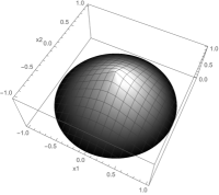
(a) $g_{0}$

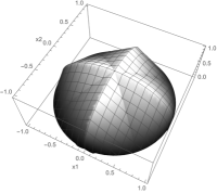
(b) $\varphi_{\mathbf{1}_{2},\mathfrak{D},1}\vee\varphi_{\mathbf{1}_{2},\mathfrak{D},2}$

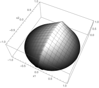
(c) $\varphi_{\mathbf{1}_{2},\mathfrak{D},1}$

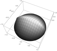
(d) $\varphi_{\mathbf{1}_{2},\mathfrak{D},2}$

Figure 1: Comparison of $g_{0}$, $\varphi_{\mathbf{1}_{2},\mathfrak{D},1}$ and $\varphi_{\mathbf{1}_{2},\mathfrak{D},2}$ on $\mathfrak{D}\equiv\{\bm{x}\in\mathbb{R}^{2}:\|\bm{x}\|_{2}<1\}$.

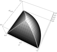
(a) $g_{0}$

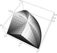
(b) $\varphi_{\mathbf{1}_{2},\mathfrak{D},1}\vee\varphi_{\mathbf{1}_{2},\mathfrak{D},2}$

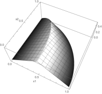
(c) $\varphi_{\mathbf{1}_{2},\mathfrak{D},1}$

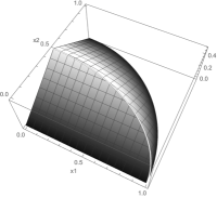
(d) $\varphi_{\mathbf{1}_{2},\mathfrak{D},2}$

Figure 2: Comparison of $g_{0}$, $\varphi_{\mathbf{1}_{2},\mathfrak{D},1}$ and $\varphi_{\mathbf{1}_{2},\mathfrak{D},2}$ on $\mathfrak{D}\equiv\{\bm{x}\in\mathbb{R}_{+}^{2}:\|\bm{x}\|_{2}<1\}$.

3.3 Examples of component-wise distances

We give the form of the component-wise distance $\bm{\varphi}_{\bm{C},\mathfrak{D}}$ for different examples of domains.

Example 1 ($\mathbb{R}^{m}$ and $\mathbb{R}_{+}^{m}$).

Two frequently encountered domains are the real space and its nonnegative orthant. These are the original settings considered in Hyvärinen (2005, 2007); Lin et al. (2016); Yu et al. (2018, 2019b). We have $\bm{\varphi}_{\bm{C},\mathbb{R}^{m}}(\bm{x})=\bm{C}$ and $\bm{\varphi}_{\bm{C},\mathbb{R}_{+}^{m}}(\bm{x})=(\min(C_{1},x_{1}),\ldots,\min(C_{m},x_{m}))$.

Example 2 (Unit hypercube).

Now consider the unit hypercube $\mathfrak{D}=[-1/2,1/2]^{m}$ as an example of a compact set and encountered in applications like (Janofsky, 2015, 2018; Tan et al., 2019). Every non-empty section $\mathfrak{C}_{j,\mathfrak{D}}\left(\bm{x}_{-j}\right)$ equals $[-1/2,1/2]$, and so $\varphi_{C_{j},\mathfrak{D},j}(\bm{x})=\min\{C_{j},1/2-|x_{j}|\}$. Since the hypercube is bounded by nature, it is natural to drop the truncation by $C_{j}$ and simply use $\bm{\varphi}_{\mathfrak{D}}(\bm{x})=\mathbf{1}_{m}/2-|\bm{x}|$.

Example 3 ($\mathcal{L}^{q}$ ball).

As a compact domain that is difficult for previously proposed approaches, consider the $\mathcal{L}^{q}$ ball with radius $r>0$ and $q\geq 1$, so $\mathfrak{D}\equiv\{\bm{x}\in\mathbb{R}^{m}:\|\bm{x}\|_{q}\leq r\}$. Given a point $\bm{x}\in\mathfrak{D}$ and an index $j\in\{1,\ldots,m\}$, the section $\mathfrak{C}_{j,\mathfrak{D}}\left(\bm{x}_{-j}\right)$ is the interval $[-(r^{q}-\mathbf{1}^{\top}|\bm{x}_{-j}|^{q})^{1/q},(r^{q}-\mathbf{1}^{\top}|\bm{x}_{-j}|^{q})^{1/q}]$, and so $\varphi_{C_{j},\mathfrak{D},j}(\bm{x})=\min\left\{C_{j},(r^{q}-\mathbf{1}^{\top}|\bm{x}_{-j}|^{q})^{1/q}-|x_{j}|\right\}$.

Example 4 ($\mathcal{L}^{q}$ ball restricted to $\mathbb{R}_{+}^{m}$).

Further restricted, consider $\mathfrak{D}\equiv\{\bm{x}\in\mathbb{R}_{+}^{m}:\|\bm{x}\|_{q}\leq r\}$, the nonnegative part of the $\mathcal{L}^{q}$ ball with radius $r>0$ and $q\geq 1$. Given a point $\bm{x}\in\mathfrak{D}$ and an index $j$, the section $\mathfrak{C}_{j,\mathfrak{D}}\left(\bm{x}_{-j}\right)$ is $[0,(r^{q}-\mathbf{1}^{\top}|\bm{x}_{-j}|^{q})^{1/q}]$, so $\varphi_{C_{j},\mathfrak{D},j}(\bm{x})=\min\left\{C_{j},x_{j},(r^{q}-\mathbf{1}^{\top}|\bm{x}_{-j}|^{q})^{1/q}-x_{j}\right\}$.

Example 5 (Complement of $\mathcal{L}^{q}$ ball).

Now consider $\mathfrak{D}\equiv\{\bm{x}\in\mathbb{R}^{m}:\|\bm{x}\|_{q}>r\}$, the complement of the $\mathcal{L}^{q}$ ball with radius $r>0$ and $q\geq 1$. Given $\bm{x}\in\mathfrak{D}$ and $j$, we now have

$$\mathfrak{C}_{j,\mathfrak{D}}\left(\bm{x}_{-j}\right)=\begin{cases}\mathbb{R}&\text{ if }\mathbf{1}_{m-1}^{\top}|\bm{x}_{-j}|^{q}>r^{q},\\ \left(-\infty,-(r^{q}-\mathbf{1}_{m-1}^{\top}|\bm{x}_{-j}|^{q})^{1/q}\right)\cup\left((r^{q}-\mathbf{1}_{m-1}^{\top}|\bm{x}_{-j}|^{q})^{1/q},+\infty\right)&\text{ otherwise};\end{cases}$$

$$\varphi_{C_{j},\mathfrak{D},j}(\bm{x})=\begin{cases}C_{j}&\text{if }\mathbf{1}_{m-1}^{\top}|\bm{x}_{-j}|^{q}>r^{q},\\ \min\left\{C_{j},|x_{j}|-(r^{q}-\mathbf{1}_{m-1}^{\top}|\bm{x}_{-j}|^{q})^{1/q}\right\}&\text{otherwise}.\end{cases}$$

Example 6 (Complement of $\mathcal{L}^{q}$ ball restricted to $\mathbb{R}_{+}^{m}$).

Next consider $\mathfrak{D}\equiv\{\bm{x}\in\mathbb{R}_{+}^{m}:\|\bm{x}\|_{q}>r\}$, the complement of the nonnegative part of the $\mathcal{L}^{q}$ ball with radius $r>0$ and $q\geq 1$. Given $\bm{x}\in\mathfrak{D}$ and $j$,

$$\mathfrak{C}_{j,\mathfrak{D}}\left(\bm{x}_{-j}\right)=\begin{cases}\mathbb{R}_{+}&\text{ if }\mathbf{1}_{m-1}^{\top}|\bm{x}_{-j}|^{q}>r^{q},\\ \left(-\infty,-(r^{q}-\mathbf{1}_{m-1}^{\top}|\bm{x}_{-j}|^{q})^{1/q}\right)\cup\left((r^{q}-\mathbf{1}_{m-1}^{\top}|\bm{x}_{-j}|^{q})^{1/q},+\infty\right)&\text{ otherwise};\end{cases}$$

$$\varphi_{C_{j},\mathfrak{D},j}(\bm{x})=\begin{cases}\min\{C_{j},x_{j}\}&\text{if }\mathbf{1}_{m-1}^{\top}|\bm{x}_{-j}|^{q}>r^{q},\\ \min\left\{C_{j},x_{j}-(r^{q}-\mathbf{1}_{m-1}^{\top}|\bm{x}_{-j}|^{q})^{1/q}\right\}&\text{otherwise}.\end{cases}$$

Example 7 (Complicated domains defined by inequality constraints).

More generally, a domain $\mathfrak{D}$ may be determined by a series of intersections/unions of regions determined by inequality constraints, e.g., $\mathfrak{D}=\{\bm{x}\in\mathbb{R}^{m}:(f_{1}(\bm{x})\leq c_{1}\wedge f_{2}(\bm{x})\leq c_{2})\vee f_{3}(\bm{x})\geq c_{3}\}$. In this case, to calculate $\bm{\varphi}_{\bm{C},\mathfrak{D}}$ we may plug in $\bm{x}_{-j}$ as given and solve numerically $f_{i}(x_{j};\bm{x}_{-j})=c_{i}$ for $i=1,2,3$, and obtain the boundary points for $x_{j}$ using simple algorithms for interval unions/intersections. This is implemented in the package genscore for some types of polynomials $f_{i}$ and arbitrary intersections/unions.

3.4 The Empirical Generalized Score Matching Loss

From this section on, we simplify notation by dropping the dependence of $\bm{\varphi}$ on $\bm{C}$ and $\mathfrak{D}$.

Lemma 1.

Suppose $\bm{C}\succ\bm{0}$, $p_{0}(\bm{x})>0$ for almost every $\bm{x}\in\mathfrak{D}$ and $h_{1}(y),\ldots,h_{m}(y)>0$ for all $y>0$. Then $J_{\bm{h},\bm{C},\mathfrak{D}}(P)=0$ if and only if $p_{0}=p$ for a.e. $\bm{x}\in\mathfrak{D}$.

Proof of Lemma 1.

By the measurability and definition of $\mathfrak{D}$, and using the Fubini-Tonelli theorem, the component-wise boundary set $\underline{\partial}\mathfrak{D}$ from Definition 1 is a Lebesgue-null set. Thus, $\bm{\varphi}(\bm{x})\succ\bm{0}$ for almost every $\bm{x}\in\mathfrak{D}$, so that $(\bm{h}\circ\bm{\varphi})(\bm{x})\succ\bm{0}$ for a.e. $\bm{x}\in\mathfrak{D}$. So $J_{\bm{h},\bm{C},\mathfrak{D}}(P)=0$ if and only if $\nabla\log p_{0}(\bm{x})=\nabla\log p(\bm{x})$ for a.e. $\bm{x}\in\mathfrak{D}$, i.e., $\log p_{0}(\bm{x})=\log p(\bm{x})+c_{0}$ for a.e. $\bm{x}\in\mathfrak{D}$ for some constant $c_{0}$, or $p_{0}(\bm{x})=c_{1}\cdot p(\bm{x})$ for a.e. $\bm{x}\in\mathfrak{D}$ for some non-zero constant $c_{1}\equiv\exp(c_{0})$. Since $p_{0}$ and $p$ both integrate to $1$ over $\mathfrak{D}$, we have $c_{1}=1$ and $p_{0}=p$ for a.e. $\bm{x}\in\mathfrak{D}$. ∎

According to Lemma 1 the proposed score matching method requires the domain $\mathfrak{D}$ to have positive Lebesgue measure in $\mathbb{R}^{m}$. For some null sets, e.g, a probability simplex, an appropriate transformation to a lower-dimensional set with positive measure can be given but we defer discussion of such domains to future work, and assume $\mathfrak{D}$ has positive Lebesgue measure for the rest of this paper.

Lemma 2.

Similar to (A0.1) and (A0.2) in Section 2.2, assume the following to hold for all $p\in\mathcal{P}(\mathfrak{D})$,

1. $p_{0}(x_{j};\bm{x}_{-j})h_{j}(\varphi_{j}(\bm{x}))\partial_{j}\log p(x_{j};\bm{x}_{-j})\left|{}_{x_{j}\searrow a_{k}(\bm{x}_{-j})^{+}}^{x_{j}\nearrow b_{k}(\bm{x}_{-j})^{-}}\right.=0$
   for all $k=1,\ldots,K_{j}(\bm{x}_{-j})$ and $\bm{x}_{-j}\in\mathfrak{S}_{-j}$ for all $j$;

2. $\int_{\mathfrak{D}}p_{0}(\bm{x})\left\|\nabla\log p(\bm{x})\odot(\bm{h}\circ\bm{\varphi})^{1/2}(\bm{x})\right\|_{2}^{2}\mathop{}\!\mathrm{d}\bm{x}<+\infty$,
   $\int_{\mathfrak{D}}p_{0}(\bm{x})\left\|\left[\nabla\log p(\bm{x})\odot(\bm{h}\circ\bm{\varphi})(\bm{x})\right]^{\prime}\right\|_{1}\mathop{}\!\mathrm{d}\bm{x}<+\infty$.

Also assume that

1. $\forall j=1,\ldots,m$ and a.e. $\bm{x}_{-j}\in\mathfrak{S}_{-j}$, the component function $h_{j}$ of $\bm{h}$ is absolutely continuous in any bounded sub-interval of the section $\mathfrak{C}_{j}(\bm{x}_{-j})$. This implies the same for $(h_{j}\circ\varphi_{j})$ and also that $\partial_{j}(h_{j}\circ\varphi_{j})$ exists a.e.

Then the loss $J_{\bm{h},\bm{C},\mathfrak{D}}(P)$ is equal to a constant depending on $p_{0}$ only (i.e., independent of $p$) plus

$$\frac{1}{2}\sum_{j=1}^{m}\int_{\mathfrak{D}}p_{0}(\bm{x})\cdot(h_{j}\circ\varphi_{j})(\bm{x})\cdot\left[\partial_{j}\log p(\bm{x})\right]^{2}\mathop{}\!\mathrm{d}\bm{x}+\sum_{j=1}^{m}\int_{\mathfrak{D}}p_{0}(\bm{x})\cdot\partial_{j}\left[(h_{j}\circ\varphi_{j})(\bm{x})\cdot\partial_{j}\log p(\bm{x})\right]\mathop{}\!\mathrm{d}\bm{x}.$$ (12)

The proof of the lemma is given in Appendix B. The lemma enables us to estimate the population loss, or rather those parts that are relevant for estimation of $P$, using the empirical loss

$$\hat{J}_{\bm{h},\bm{C},\mathfrak{D}}(P)=\frac{1}{2}\sum_{j=1}^{m}\sum_{i=1}^{n}\frac{1}{2}(h_{j}\circ\varphi_{j})\left(\bm{x}^{(i)}\right)\cdot\left[\partial_{j}\log p\left(\bm{x}^{(i)}\right)\right]^{2}+\partial_{j}\left[(h_{j}\circ\varphi_{j})\left(\bm{x}^{(i)}\right)\cdot\partial_{j}\log p\left(\bm{x}^{(i)}\right)\right].$$ (13)

As the canonical choices of $\bm{h}$ are power functions in $\bm{x}$, we give the following sufficient conditions for the assumptions in the lemma.

Proposition 3.

Suppose for all $j=1,\ldots,m$, $h_{j}(x_{j})=x_{j}^{\alpha_{j}}$ for some $\alpha_{j}>0$. Suppose in addition that for all $j$ and $\bm{x}_{-j}\in\mathfrak{S}_{-j}$ and all $p\in\mathcal{P}$ we have

1. $p_{0}(x_{j};\bm{x}_{-j})\partial_{j}\log p(x_{j};\bm{x}_{-j})=o\left(1/(x_{j}-c_{k,j})^{\alpha_{j}}\right)$ as $x_{j}\nearrow c_{k,j}\equiv b_{k,j}(\bm{x}_{-j})<+\infty$ or as $x_{j}\searrow c_{k,j}\equiv a_{k,j}(\bm{x}_{-j})>-\infty$ for all $k$, and

2. $p_{0}(x_{j};\bm{x}_{-j})\partial_{j}\log p(x_{j};\bm{x}_{-j})\to 0$ as $x_{j}\nearrow+\infty$ if $\mathfrak{C}_{j}(\bm{x}_{-j})$ is unbounded from above, and as $x_{j}\searrow-\infty$ if $\mathfrak{C}_{j}(\bm{x}_{-j})$ is unbounded from below.

Then (A.1) and (A.3) are satisfied.

Proof of Proposition 3.

Condition (A.3) is satisfied by the property of $h_{j}$. (A.1) is also satisfied since by construction $(h_{j}\circ\varphi_{j})(\bm{x})$ becomes $|x_{j}-c_{k,j}|^{\alpha_{j}}$ as $x_{j}\to c_{k,j}\in\cup_{k=1}^{K_{j}}\{a_{k,j}(\bm{x}_{-j}),b_{k,j}(\bm{x}_{-j})\}$ and also $(h_{j}\circ\varphi_{j})$ is bounded by $C^{\alpha_{j}}$ as $x_{j}\nearrow+\infty$ or $x_{j}\searrow-\infty$, if applicable. ∎

3.5 Exponential Families and Regularized Score Matching

Consider the case where $\mathcal{P}(\mathfrak{D})\equiv\{p_{\bm{\theta}}:\bm{\theta}\in\bm{\Theta}\subset\mathbb{R}^{r}\}$ for some $r=1,2,\ldots$ is an exponential family comprised of continuous distributions supported on $\mathfrak{D}$ with densities of the form

$$\log p_{\bm{\theta}}(\bm{x})=\bm{\theta}^{\top}\bm{t}(\bm{x})-\psi(\bm{\theta})+b(\bm{x}),\quad\bm{x}\in\mathfrak{D},$$ (14)

where $\bm{\theta}\in\mathbb{R}^{r}$ is the unknown canonical parameter of interest, $\bm{t}(\bm{x})\in\mathbb{R}^{r}$ are the sufficient statistics, $\psi(\bm{\theta})$ is the normalizing constant, and $b(\bm{x})$ is the base measure. The empirical loss $\hat{J}_{\bm{h},\bm{C},\mathfrak{D}}$ (13) can then be written as a quadratic function in the canonical parameter:

$$\hat{J}_{\bm{h},\bm{C},\mathfrak{D}}(p_{\bm{\theta}}) =\frac{1}{2}\bm{\theta}^{\top}\bm{\Gamma}(\mathbf{x})\bm{\theta}-\bm{g}(\mathbf{x})^{\top}\bm{\theta}+\mathrm{const},\quad\text{with}$$ (15)

$$\bm{\Gamma}(\mathbf{x}) =\frac{1}{n}\sum_{i=1}^{n}\sum_{j=1}^{m}(h_{j}\circ\varphi_{j})\left(\bm{X}^{(i)}\right)\partial_{j}\bm{t}(\bm{X}^{(i)})\left(\partial_{j}\bm{t}\left(\bm{X}^{(i)}\right)\right)^{\top}\quad\text{and}$$ (16)

$$\bm{g}(\mathbf{x}) =-\frac{1}{n}\sum_{i=1}^{n}\sum_{j=1}^{m}\left[(h_{j}\circ\varphi_{j})\left(\bm{X}^{(i)}\right)\partial_{j}b\left(\bm{X}^{(i)}\right)\partial_{j}\bm{t}\left(\bm{X}^{(i)}\right)\right.$$

$$\quad\left.+(h_{j}\circ\varphi_{j})\left(\bm{X}^{(i)}\right)\partial_{jj}\bm{t}\left(\bm{X}^{(i)}\right)+\partial_{j}(h_{j}\circ\varphi_{j})\left(\bm{X}^{(i)}\right)\partial_{j}\bm{t}\left(\bm{X}^{(i)}\right)\right],$$ (17)

where $\partial_{j}\bm{t}(\bm{x})=(\partial_{j}t_{1}(\bm{x}),\ldots,\partial_{j}t_{r}(\bm{x}))^{\top}\in\mathbb{R}^{r}$. Note that (16) and (17) are sample averages of functions in the data matrix $\mathbf{x}$ only. These forms are an exact analog of those in Theorem 5 in Yu et al. (2019b). As expected, we can thus obtain the following consistency result similar to Theorem 6 in Yu et al. (2019b):

Theorem 4 (Theorem 6 of Yu et al. (2019b)).

Suppose the true density is $p_{0}\equiv p_{\bm{\theta}_{0}}$ and that

1. $\bm{\Gamma}$ is almost surely invertible, and

2. $\bm{\Sigma}_{0}\equiv\mathbb{E}_{p_{0}}\left[\left(\bm{\Gamma}(\mathbf{x})\bm{\theta}_{0}-\bm{g}(\mathbf{x})\right)\left(\bm{\Gamma}(\mathbf{x})\bm{\theta}_{0}-\bm{g}(\mathbf{x})\right)^{\top}\right]$, $\bm{\Gamma}_{0}\equiv\mathbb{E}_{p_{0}}\bm{\Gamma}(\mathbf{x})$, $\bm{\Gamma}_{0}^{-1}$, and $\bm{g}_{0}\equiv\mathbb{E}_{p_{0}}\bm{g}(\mathbf{x})$ exist and are component-wise finite.

Then the minimizer of (15) is almost surely unique with closed form solution $\hat{\bm{\theta}}\equiv\bm{\Gamma}(\mathbf{x})^{-1}\bm{g}(\mathbf{x})$ with

$$\hat{\bm{\theta}}\to_{\text{a.s.}}\bm{\theta}_{0}\quad\text{and}\quad\sqrt{n}(\hat{\bm{\theta}}-\bm{\theta}_{0})\to_{d}\mathcal{N}_{r}\left(\bm{0},\bm{\Gamma}_{0}^{-1}\bm{\Sigma}_{0}\bm{\Gamma}_{0}^{-1}\right)\quad\text{as }n\to\infty.$$

Estimation in high-dimensional settings, in which the number of parameters $r$ may exceed the sample size $n$, usually benefits from regularization. For exponential families, as in Yu et al. (2019b), we add an $\ell_{1}$ penalty on $\bm{\theta}$ to the loss in (15), while multiplying the diagonals of the $\bm{\Gamma}$ by a diagonal multiplier $\delta>1$:

Definition 4.

Let $\delta>1$, and $\bm{\Gamma}_{\delta}(\mathbf{x})$ be $\bm{\Gamma}(\mathbf{x})$ with diagonal entries multiplied by $\delta$. For exponential family distributions in (14), the regularized generalized $(\bm{h},\bm{C},\mathfrak{D})$-score matching loss is defined as

$$\hat{J}_{\bm{h},\bm{C},\mathfrak{D},\lambda,\delta}(p_{\bm{\theta}})\equiv\frac{1}{2}\bm{\theta}^{\top}\bm{\Gamma}_{\delta}(\mathbf{x})\bm{\theta}-\bm{g}(\mathbf{x})^{\top}\bm{\theta}+\lambda\|\bm{\theta}\|_{1}.$$ (18)

The multiplier $\delta>1$, together with the $\ell_{1}$ penalty, resembles an elastic net penalty and prevents the loss in (18) from being unbounded from below for smaller $\lambda$, in which case there can be infinitely many minimizers. This is discussed in Section 4 in Yu et al. (2019b), where a default for $\delta$ is given, so that no tuning for this parameter is necessary. Minimization of (18) can be efficiently done using coordinate-descent with warm starts, which along with other computational details is discussed in Section 5.3 of Yu et al. (2019b).

3.6 Extension of the Method from Liu and Kanamori (2019) to Unbounded Domains

A key ingredient to our treatment of unbounded domains is truncation of distances. This idea can also be applied to the method proposed for general bounded domains in Liu and Kanamori (2019); recall Section 2.3. For any component-wise countable union of intervals $\mathfrak{D}$ as in Definition 1, we may modify the loss in (6) to

$$J_{g_{0},C,\mathfrak{D}}(P)\equiv\sup_{g\in\mathcal{G}}\frac{1}{2}\int_{\mathbb{R}_{+}^{m}}g(\bm{x})p_{0}(\bm{x})\left\|\nabla\log p(\bm{x})-\nabla\log p_{0}(\bm{x})\right\|_{2}^{2}\mathop{}\!\mathrm{d}\bm{x},$$

but with $\mathcal{G}\equiv\{g|g(\bm{x})=0,\forall\bm{x}\in\underline{\partial}\mathfrak{D},\,g\text{ is }L\text{-Lipschitz continuous}\text{ and }g\leq C\}$ instead. Here, we use the same Lipschitz constant $L>0$ but add an extra truncation constant $C>0$. Moreover, we use the component-wise boundary set $\underline{\partial}\mathfrak{D}$ (8) instead of the usual boundary set $\partial\mathfrak{D}$ used in Liu and Kanamori (2019). Following the same proof as for their Proposition 1 and dropping the Lipschitz constant $L$ by replacing $C$ with $C/L$ (or equivalently choosing $L=1$), it is easy to see that the maximum is obtained at

$$g_{0}(\bm{x})\equiv\min\left\{C,\inf_{\bm{x}^{\prime}\in\underline{\partial}\mathfrak{D}}\|\bm{x}-\bm{x}^{\prime}\|_{2}\right\},$$ (19)

the $\ell_{2}$ distance of $\bm{x}$ to $\underline{\partial}\mathfrak{D}$ truncated above by $C$, which naturally extends the method in Liu and Kanamori (2019) to unbounded domains. In the special case where $\underline{\partial}\mathfrak{D}=\varnothing$, we must have $\mathfrak{D}\equiv\mathbb{R}^{m}$ and $g_{0}(\bm{x})\equiv C$ by the expression above (with the convention of $\inf\varnothing=+\infty$), which coincides with the original score matching in Hyvärinen (2005).

Assuming that (A.1) and (A.2) from Lemma 2 hold when replacing $(\bm{h}\circ\bm{\varphi})(\bm{x})$ by $g_{0}(\bm{x})\mathbf{1}_{m}$ and $h_{j}(\varphi_{j}(\bm{x}))$ by $g_{0}(\bm{x})$, the same conclusion there applies, i.e.

$$J_{g_{0},C,\mathfrak{D}}(P)\equiv\frac{1}{2}\sum_{j=1}^{m}\int_{\mathfrak{D}}p_{0}(\bm{x})g_{0}(\bm{x})\left[\partial_{j}\log p(\bm{x})\right]^{2}\mathop{}\!\mathrm{d}\bm{x}+\sum_{j=1}^{m}\int_{\mathfrak{D}}p_{0}(\bm{x})\partial_{j}\left[g_{0}(\bm{x})\partial_{j}\log p(\bm{x})\right]\mathop{}\!\mathrm{d}\bm{x}$$

plus a constant depending on $p_{0}$ but not on $p$; this is the same loss as in Equation (13) in Liu and Kanamori (2019) with a truncation by $C$ applied to $g_{0}$. The proof is in the same spirit of that for Lemma 2 and is thus omitted.

4 Pairwise Interaction Models on Domains with Positive Measure

4.1 Pairwise Interaction Power $a$-$b$ Models

As one realm of application of the proposed estimation method, we consider exponential family models that postulate pairwise interactions between power-transformations of the observed variables, as in (4):

$$p_{\bm{\eta},\mathbf{K}}(\bm{x})\propto\exp\left(-\frac{1}{2a}{\bm{x}^{a}}^{\top}\mathbf{K}\bm{x}^{a}+\frac{1}{b}\bm{\eta}^{\top}\bm{x}^{b}\right)\mathds{1}_{\mathfrak{D}}(\bm{x})$$ (20)

for which we treat $\bm{x}^{0}\equiv\log\bm{x}$ and $1/0\equiv 1$, on a domain $\mathfrak{D}\subseteq\mathbb{R}^{m}$ with a positive measure. Here $a\geq 0$ and $b\geq 0$ are known constants and the interaction matrix $\mathbf{K}\in\mathbb{R}^{m\times m}$ and the linear vector $\bm{\eta}\in\mathbb{R}^{m}$ are unknown parameters of interest. As in Yu et al. (2019b), our focus will be on the support of $\mathbf{K}$, $S(\mathbf{K})=\{(i,j):\kappa_{ij}\neq 0\}$, that for product domains defines the conditional independence graph of $\bm{X}\sim p_{\bm{\eta},\mathbf{K}}$. However, we simultaneously estimate the nuisance parameter $\bm{\eta}$ unless it is explicitly assumed to be $\mathbf{0}$.

When $a=b=1$, model (20) is a truncated Gaussian model. From $a=b=1/2$, we may obtain the exponential square-root graphical model in Inouye et al. (2016). The gamma model in Yu et al. (2019b) has $a=1/2$ and $b=0$.

4.2 Finite Normalizing Constant and Validity of Score Matching

The following theorem gives detailed sufficient conditions for the $a$-$b$ density $p_{\bm{\eta},\mathbf{K}}$ in (20) to be a proper density on a domain $\mathfrak{D}\subseteq\mathbb{R}^{m}$ with positive Lebesgue measure.

Theorem 5 (Sufficient conditions for finite normalizing constant).

Denote $\rho_{j}(\mathfrak{D})\equiv\overline{\{x_{j}:\bm{x}\in\mathfrak{D}\}}$ the closure of the range of $x_{j}$ in the domain $\mathfrak{D}$. If any of the following conditions holds, the density in (20) is a proper density, i.e., the right-hand of (20) is integrable over $\mathfrak{D}$:

1. $a>0$, $b>0$, $\mathfrak{D}$ is bounded;

2. $a>0$, $b>0$, ${\bm{v}^{a}}^{\top}\mathbf{K}\bm{v}^{a}>0\,\,\forall\bm{v}\in\mathfrak{D}\backslash\{\bm{0}\}$, and either $2a>b$ or $\bm{\eta}^{\top}\bm{v}^{b}\leq 0$ $\forall\bm{v}\in\mathfrak{D}$;

3. $a>0$, $b=0$, $\eta_{j}>-1$ for all $j$ s.t. $0\in\rho_{j}(\mathfrak{D})$, and one of the following holds:

   1. $\mathfrak{D}$ is bounded;

   2. $\mathfrak{D}$ is unbounded and ${\bm{v}^{a}}^{\top}\mathbf{K}\bm{v}^{a}>0\,\,\forall\bm{v}\in\mathfrak{D}\backslash\{\bm{0}\}$;

   3. $\mathfrak{D}$ is unbounded, ${\bm{v}^{a}}^{\top}\mathbf{K}\bm{v}^{a}\geq 0\,\,\forall\bm{v}\in\mathfrak{D}$ and $\eta_{j}<-1$ for all $j$ s.t. $\rho_{j}(\mathfrak{D})$ is unbounded (which implies that $\rho_{j}(\mathfrak{D})=[0,+\infty)$ is not allowed for any $j$);

4. $a=0$, $\mathfrak{D}$ is bounded and $0\not\in\rho_{j}(\mathfrak{D})$ for all $j$;

5. $a=0$, $b=0$, $\log(\bm{x})^{\top}\mathbf{K}\log(\bm{x})>0$ $\forall\bm{x}\in\mathfrak{D}$;

6. $a=0$, $b>0$, $\log(\bm{x})^{\top}\mathbf{K}\log(\bm{x})>0$ $\forall\bm{x}\in\mathfrak{D}$ and $\eta_{j}\leq 0$ for all $j$ s.t. $\rho_{j}(\mathfrak{D})$ is unbounded;

7. $a=0$, $b>0$, $\log(\bm{x})^{\top}\mathbf{K}\log(\bm{x})\geq 0$ $\forall\bm{x}\in\mathfrak{D}$ and $\eta_{j}<0$ for all $j$ s.t. $\rho_{j}(\mathfrak{D})$ is unbounded.

In the centered case where $\bm{\eta}=\bm{0}$ is known, any condition in terms of $b$ and $\bm{\eta}$ can be ignored.

To simplify our discussion, the following corollary gives a simpler set of sufficient conditions for integrability of the density.

Corollary 6 (Sufficient conditions for finite normalizing constant; simplified).

Suppose

1. $\mathbf{K}$ is positive definite

and one of the following conditions holds:

1. $2a>b>0$ or $a=b=0$;

2. $a>0$, $b=0$, $\bm{\eta}\succ-\mathbf{1}_{m}$;

3. $a=0$, $b>0$, $\eta_{j}\leq 0$ for any $j$ such that $x_{j}$ is unbounded in $\mathfrak{D}$.

Then the right-hand side of (20) is integrable over $\mathfrak{D}$. In the case where $\bm{\eta}\equiv\bm{0}$, (CC0*) is sufficient.

For simplicity, we use conditions (CC0*)–(CC3*) throughout the paper. The following theorem gives sufficient conditions on $\bm{h}$ that satisfy conditions (A.1)–(A.3) in Lemma 2 for score matching.

Theorem 7 (Sufficient conditions that satisfy assumptions for score matching).

Suppose (CC0*) and one of (CC1*) through (CC3*) holds, and $\bm{h}(\bm{x})=\left(x_{1}^{\alpha_{1}},\ldots,x_{m}^{\alpha_{m}}\right)$, where

1. if $a>0$ and $b>0$, $\alpha_{j}>\max\{0,1-a,1-b\}$;

2. if $a>0$ and $b=0$, $\alpha_{j}>1-\eta_{0,j}$;

3. if $a=0$, $\alpha_{j}\geq 0$.

Then conditions (A.1), (A.2) and (A.3) in Lemma 2 are satisfied and the equivalent form of the generalized score matching loss (12) holds, and the empirical loss (13) is valid. In the centered case with $\bm{\eta}\equiv\bm{0}$, it suffices to have $a>0$ and $\alpha_{j}>\max\{0,1-a\}$ or $a=0$ and $\alpha_{j}\geq 0$.

4.3 Estimation

Let $\bm{\Psi}\equiv\left[\mathbf{K}^{\top}\,\,\bm{\eta}\right]^{\top}\in\mathbb{R}^{(m+1)\times m}$. In this section, we give the form of $\bm{\Gamma}\in\mathbb{R}^{(m+1)m\times(m+1)m}$ and $\bm{g}\in\mathbb{R}^{(m+1)m}$ in the unpenalized loss $\frac{1}{2}\mathrm{vec}(\bm{\Psi})^{\top}\bm{\Gamma}\mathrm{vec}(\bm{\Psi})-\bm{g}^{\top}\mathrm{vec}(\bm{\Psi})$ following (16)–(17). $\bm{\Gamma}$ is block-diagonal, with the $j$-th $\mathbb{R}^{(m+1)\times(m+1)}$ block

$$\bm{\Gamma}_{j}(\mathbf{x}) \equiv\begin{bmatrix}\bm{\Gamma}_{\mathbf{K},j}&\bm{\gamma}_{\mathbf{K},\bm{\eta},j}\\ \bm{\gamma}_{\mathbf{K},\bm{\eta},j}^{\top}&{\gamma}_{\bm{\eta},j}\end{bmatrix}$$

$$\equiv\frac{1}{n}\sum\limits_{i=1}^{n}\begin{bmatrix}(h_{j}\circ\varphi_{j})\left(\bm{X}^{(i)}\right){X_{j}^{(i)}}^{2a-2}{\bm{X}^{(i)}}^{a}{{\bm{X}^{(i)}}^{a}}^{\top}&-(h_{j}\circ\varphi_{j})\left(\bm{X}^{(i)}\right){X_{j}^{(i)}}^{a+b-2}{\bm{X}^{(i)}}^{a}\\ -(h_{j}\circ\varphi_{j})\left(\bm{X}^{(i)}\right){X_{j}^{(i)}}^{a+b-2}{{\bm{X}^{(i)}}^{a}}^{\top}&(h_{j}\circ\varphi_{j})\left(\bm{X}^{(i)}\right){X_{j}^{(i)}}^{2b-2}\end{bmatrix}.$$

On the other hand, $\bm{g}\equiv\mathrm{vec}\left(\left[\mathbf{g}_{\mathbf{K}}^{\top}\,\,\,\,\bm{g}_{\bm{\eta}}\right]^{\top}\right)\in\mathbb{R}^{(m+1)m}$, where $\mathbf{g}_{\mathbf{K}}\in\mathbb{R}^{m\times m}$ and $\bm{g}_{\bm{\eta}}\in\mathbb{R}^{m}$ correspond to $\mathbf{K}$ and $\bm{\eta}$, respectively. The $j$-th column of $\mathbf{g}_{\mathbf{K}}$ is

$$\frac{1}{n}\sum_{i=1}^{n}\left(\partial_{j}(h_{j}\circ\varphi_{j})\left(\bm{X}^{(i)}\right){X_{j}^{(i)}}^{a-1}+(a-1)(h_{j}\circ\varphi_{j})\left(\bm{X}^{(i)}\right){X_{j}^{(i)}}^{a-2}\right){\bm{X}^{(i)}}^{a}\\ +a(h_{j}\circ\varphi_{j})\left(\bm{X}^{(i)}\right){X_{j}^{(i)}}^{2a-2}\bm{e}_{j,m},$$ (21)

where $\bm{e}_{j,m}\in\mathbb{R}^{m}$ has $1$ at the $j$-th component and 0 elsewhere, and the $j$-th entry of $\bm{g}_{\bm{\eta}}$ is

$$\frac{1}{n}\sum_{i=1}^{n}-\partial_{j}(h_{j}\circ\varphi_{j})\left(\bm{X}^{(i)}\right){X_{j}^{(i)}}^{b-1}-(b-1)(h_{j}\circ\varphi_{j})\left(\bm{X}^{(i)}\right){X_{j}^{(i)}}^{b-2}.$$ (22)

If $a=0$, set the coefficients $(a-1)$ to $-1$ and $a$ to $1$ in (21); for $b=0$ set $(b-1)$ to $-1$ in the second term of (22).

As in Yu et al. (2019b) we only apply the diagonal multiplier $\delta$ to the diagonals of $\bm{\Gamma}_{\mathbf{K},j}\in\mathbb{R}^{m\times m}$, not $\gamma_{\bm{\eta},j}\in\mathbb{R}$. Note that each block of $\bm{\Gamma}$ and $\bm{g}$ correspond to each column of $\bm{\Psi}$, i.e. $(\bm{\kappa}_{,j},\eta_{j})\in\mathbb{R}^{m+1}$. In the penalized generalized score-matching loss (18), the penalty $\lambda$ for $\mathbf{K}$ and $\bm{\eta}$ can be different, $\lambda_{\mathbf{K}}$ and $\lambda_{\bm{\eta}}$, respectively, as long as the ratio $\lambda_{\bm{\eta}}/\lambda_{\mathbf{K}}$ is fixed. For $\mathbf{K}$ we follow the convention that we penalize its off-diagonal entries only. That is,

$$\frac{1}{2}\mathrm{vec}(\bm{\Psi})^{\top}{\bm{\Gamma}}_{\delta}(\mathbf{x})\mathrm{vec}(\bm{\Psi})-{\bm{g}}(\mathbf{x})^{\top}\mathrm{vec}(\bm{\Psi})+\lambda_{\mathbf{K}}\|\mathbf{K}_{\mathrm{off}}\|_{1}+\lambda_{\bm{\eta}}\|\bm{\eta}\|_{1}.$$ (23)

In the case where we do not penalize $\bm{\eta}$, i.e. $\lambda_{\bm{\eta}}=0$, we can simply profile out $\bm{\eta}$, solve for $\hat{\bm{\eta}}=\bm{\Gamma}_{\bm{\eta}}^{-1}\left(\bm{g}_{\bm{\eta}}-\bm{\Gamma}_{\mathbf{K},\bm{\eta}}^{\top}\mathrm{vec}(\hat{\mathbf{K}})\right)$, plug this back in and rewrite the loss in $\mathbf{K}$ only. Let $\bm{\Gamma}_{\delta,\mathbf{K}}\in\mathbb{R}^{m^{2}\times m^{2}}$ be the block-diagonal matrix with blocks $\bm{\Gamma}_{\mathbf{K},j}$ and diagonal multiplier $\delta$, and let $\bm{\Gamma}_{\mathbf{K},\bm{\eta}}\in\mathbb{R}^{m^{2}\times m}$ and $\bm{\Gamma}_{\bm{\eta}}\in\mathbb{R}^{m\times m}$ be the (block-)diagonal matrices with blocks $\bm{\gamma}_{\mathbf{K},\bm{\eta},j}$ and $\gamma_{\bm{\eta},j}$, respectively. Denote $\bm{\Gamma}_{\delta,\mathrm{profiled}}$ as the Schur complement of $\bm{\Gamma}_{\delta,\mathbf{K}}$ of $\left[\begin{smallmatrix}\bm{\Gamma}_{\delta,\mathbf{K}}&\bm{\Gamma}_{\mathbf{K},\bm{\eta}}\\ \bm{\Gamma}_{\mathbf{K},\bm{\eta}}^{\top}&\bm{\Gamma}_{\bm{\eta}}\end{smallmatrix}\right]$, i.e. $\bm{\Gamma}_{\delta,\mathbf{K}}-\bm{\Gamma}_{\mathbf{K},\bm{\eta}}\bm{\Gamma}_{\bm{\eta}}^{-1}\bm{\Gamma}_{\mathbf{K},\bm{\eta}}^{\top}$, which is guaranteed to be positive definite for $\delta>1$. Then the profiled loss is

$$\hat{J}_{\bm{h},\bm{C},\mathfrak{D},\lambda,\delta,\mathrm{profiled}}(p_{\mathbf{K}})\equiv\frac{1}{2}\mathrm{vec}(\mathbf{K})^{\top}\bm{\Gamma}_{\delta,\mathrm{profiled}}\mathrm{vec}(\mathbf{K})-\left(\bm{g}_{\mathbf{K}}-\bm{\Gamma}_{\mathbf{K},\bm{\eta}}\bm{\Gamma}_{\bm{\eta}}^{-1}\bm{g}_{\bm{\eta}}\right)^{\top}\mathrm{vec}(\mathbf{K})+\lambda_{\mathbf{K}}\|\mathbf{K}\|_{1}.$$ (24)

4.4 Univariate Examples

To illustrate our generalized score matching framework, we first present univariate Gaussian models on a general domain $\mathfrak{D}\subset\mathbb{R}$ that is a countable union of intervals and has positive Lebesgue measure. In particular, we estimate one of $\mu_{0}$ and $\sigma_{0}^{2}$ assuming the other is known, given that the true density is

$$p_{\mu_{0},\sigma_{0}^{2}}(x)\propto\exp\left\{-\frac{(x-\mu_{0})^{2}}{2\sigma_{0}^{2}}\right\},\quad x\in\mathfrak{D},$$

with $\mu_{0}\in\mathbb{R}$ and $\sigma_{0}^{2}>0$. Let $X^{(1)},\ldots,X^{(n)}\sim p_{\mu_{0},\sigma_{0}^{2}}$ be i.i.d. samples. Without any regularization by an $\ell_{1}$ or $\ell_{2}$ penalty and assuming the true $\sigma_{0}^{2}$ is known, we have similar to Example 3.1 in Yu et al. (2019b) that our generalized score matching estimator for $\mu_{0}$ is

$$\hat{\mu}\equiv\frac{\sum_{i=1}^{n}(h\circ\varphi_{C})\left(X^{(i)}\right)\cdot X^{(i)}-\sigma_{0}^{2}(h\circ\varphi_{C})^{\prime}\left(X^{(i)}\right)}{\sum_{i=1}^{n}(h\circ\varphi_{C})\left(X^{(i)}\right)}.$$

By Theorem 7, it suffices to choose $h(x)=x^{\alpha}$ with $\alpha>0$. Similar to Yu et al. (2019b), we have

$$\sqrt{n}\left(\hat{\mu}-\mu_{0}\right)\to_{d}\mathcal{N}\left(0,\frac{\mathbb{E}_{0}\left[\sigma_{0}^{2}(h\circ\varphi_{C})^{2}(X)+\sigma_{0}^{4}{(h\circ\varphi_{C})^{\prime}}^{2}(X)\right]}{\mathbb{E}_{0}^{2}\left[(h\circ\varphi_{C})(X)\right]}\right),$$ (25)

if the expectations exist. On the other hand, assuming the true $\mu_{0}$ is known, the estimator for $\sigma^{2}$ is

$$\hat{\sigma}^{2}\equiv\frac{\sum_{i=1}^{n}(h\circ\varphi_{C})\left(X^{(i)}\right)\cdot\left(X^{(i)}-\mu_{0}\right)^{2}}{\sum_{i=1}^{n}(h\circ\varphi_{C})\left(X^{(i)}\right)+(h\circ\varphi_{C})^{\prime}\left(X^{(i)}\right)\cdot\left(X^{(i)}-\mu_{0}\right)},\text{ with limiting distribution}$$

$$\sqrt{n}\left(\hat{\sigma}^{2}-\sigma_{0}^{2}\right)\to_{d}\mathcal{N}\left(0,\frac{\mathbb{E}_{0}\left[2\sigma_{0}^{6}(h\circ\varphi_{C})^{2}(X)\cdot(X-\mu_{0})^{2}+\sigma^{8}_{0}{(h\circ\varphi_{C})^{\prime}}^{2}(X)\cdot(X-\mu_{0})^{2}\right]}{\mathbb{E}_{0}^{2}\left[(h\circ\varphi_{C})(X)\cdot(X-\mu_{0})^{2}\right]}\right).$$ (26)

Figure 3 shows a standard normal distribution $\mathcal{N}(0,1)$ restricted to three univariate domains: $\mathfrak{D}_{2}\equiv(-\infty,-3/2]\cup[3/2,+\infty)$, $\mathfrak{D}_{3}\equiv[-1,-3/4]\cup[3/4,1]$, and their union $\mathfrak{D}_{1}\equiv(-\infty,-3/2]\cup[-1,-3/4]\cup[3/4,1]\cup[3/2,+\infty)$. The endpoints are chosen so that the probability of the variable lying in each interval is roughly the same: $\mathcal{N}(0,1)\left((-\infty,-3/2]\right)\approx 0.0668$ and $\mathcal{N}(0,1)\left([-1,-3/4]\right)\approx 0.0680$. To pick the truncation point $C$ for the distance $\varphi_{C,\mathfrak{D}}$, we choose $\pi\in(0,1]$ and let $C$ be the $\pi$ quantile of the distribution of $\varphi_{+\infty,\mathfrak{D}}(X)$, where the random variable $X$ follows the truncation of $\mathcal{N}(0,1)$ to the domain $\mathfrak{D}$. So, $C$ is such that $\mathbb{P}\left(\varphi_{+\infty,\mathfrak{D}}(X)\leq C\right)=\pi$. Here, $\varphi_{+\infty,\mathfrak{D}_{1}}(X)=|X|-3/2$ if $|X|>3/2$, or $\min(|X|-3/4,1-|X|)$ otherwise, $\varphi_{+\infty,\mathfrak{D}_{2}}(X)=|X|-3/2$, and $\varphi_{+\infty,\mathfrak{D}_{3}}(X)=\min(|X|-3/4,1-|X|)$.

The first subfigure in each row of Figure 3 shows the density on each domain, along with the corresponding $\varphi_{+\infty}(X)$ in red, whose $y$ axis is on the right. The second plot in each row shows the log asymptotic variance for the corresponding $\hat{\mu}$, as on the right-hand side of (25), and the third shows that for $\hat{\sigma}^{2}$ as in (26). Each curve represents a different $\alpha$ in $h(x)=x^{\alpha}$, and the $x$ axis represents the quantiles $\pi$ associated with the truncation point $C$ as above. Finally, the red dotted curve shows $C$ versus $\pi$ for each domain. The “bumps” in the variance for $x^{0.5}$ are due to numerical instability in integration.

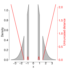
(a) Density on $\mathfrak{D}_{1}$

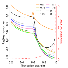
(b) Asymptotic $\log\mathrm{var}\left(\hat{\mu}\right)$ for $\mathfrak{D}_{1}$

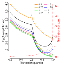
(c) Asymptotic $\log\mathrm{var}\left(\hat{\sigma}^{2}\right)$ for $\mathfrak{D}_{1}$

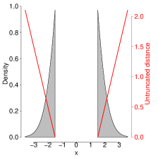
(d) Density on $\mathfrak{D}_{2}$

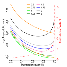
(e) Asymptotic $\log\operatorname{var}\left(\hat{\mu}\right)$ for $\mathfrak{D}_{2}$

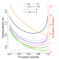
(f) Asymptotic $\log\operatorname{var}\left(\hat{\sigma}^{2}\right)$ for $\mathfrak{D}_{2}$

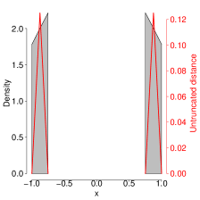
(g) Density on $\mathfrak{D}_{3}$

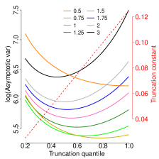
(h) Asymptotic $\log\operatorname{var}\left(\hat{\mu}\right)$ for $\mathfrak{D}_{3}$

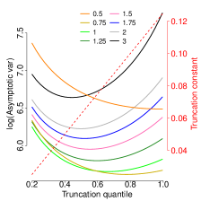
(i) Asymptotic $\log\operatorname{var}\left(\hat{\sigma}^{2}\right)$ for $\mathfrak{D}_{3}$

Figure 3: Univariate Gaussian example. Each row represents a domain, with the first subfigure plotting the density, the second the asymptotic log variance of $\hat{\mu}$, the third that of $\hat{\sigma}^{2}$. In each first subfigure the red lines show the untruncated distances $\varphi_{+\infty}$ for each domain, and the red dotted lines in the second and third show the truncation point $C$ versus the $\pi$ quantile.

As we show in Section 5, for the purpose of edge recovery for graphical models, we recommend using $\bm{h}(\bm{x})=\left(x_{1}^{\alpha_{1}},\ldots,x_{m}^{\alpha_{m}}\right)$ with $\alpha\geq 1$ for $\mathfrak{D}$ that is a finite disjoint union of convex subsets of $\mathbb{R}^{m}$. Although minimizing the asymptotic variance in the univariate case is a different task, $\alpha=1$ also seems to be consistently the best performing choice.

For $\mathfrak{D}_{2}$ and $\mathfrak{D}_{3}$, all variance curves are U-shaped, while for $\mathfrak{D}_{1}=\mathfrak{D}_{2}\cup\mathfrak{D}_{3}$ we see two such curves piecewise connected at $C_{0}=\max\varphi_{+\infty,\mathfrak{D}_{3}}(x)=(1-3/4)/2=0.125$. To the right of $C_{0}$, the truncation is applied to the two unbounded intervals (i.e. $\mathfrak{D}_{2}$) only. The first segments of most $\mathrm{var}(\hat{\mu})$ curves for $\mathfrak{D}_{1}$ as well as most curves for $\mathfrak{D}_{2}$ indicate there might still be benefit from truncating the distances $\varphi$ within the bounded intervals, although the $\mathrm{var}\left(\hat{\sigma}^{2}\right)$ curves for $\mathfrak{D}_{1}$ as well as both curves for $x^{0.75}$ on $\mathfrak{D}_{2}$ suggest otherwise. On the other hand, the curves for $\mathfrak{D}_{1}$ and $\mathfrak{D}_{2}$ imply that a truncation constant larger than $C_{0}$ is favorable; the ticks on the right-hand side indicate that the curves for $\mathfrak{D}_{2}$ reach their minimum at $C\geq 0.5$. Hence, a separate truncation point $C$ for each connected component of $\mathfrak{D}$ could be beneficial, especially for unbounded sets. However, the necessary tuning of multiple parameters becomes infeasible for $m\gg 1$ and we do not further examine it in this paper.

5 Theoretical Properties

This section presents theoretical guarantees for our generalized method applied to the pairwise interaction power $a$-$b$ models. We first state a result analogous to Yu et al. (2019b) for truncated Gaussian densities on a general domain $\mathfrak{D}$, and then present a general result for $a$-$b$ models. In particular, similar to and as a generalization of Yu et al. (2019b), we give a high probability bound on the deviation of our estimates $\hat{\mathbf{K}}$ and $\hat{\bm{\eta}}$ from their true values $\mathbf{K}_{0}$ and $\bm{\eta}_{0}$. The main challenge in deriving the results lies in obtaining marginal probability tail bounds of each observed value in $\bm{\Gamma}$ and $\bm{g}$. We first restate Definition 12 from Yu et al. (2019b).

Definition 5.

Let $\bm{\Gamma}_{0}\equiv\mathbb{E}_{0}\bm{\Gamma}(\mathbf{x})$ and $\bm{g}_{0}\equiv\mathbb{E}_{0}\bm{g}(\mathbf{x})$ be the population versions of $\bm{\Gamma}(\mathbf{x})$ and $\bm{g}(\mathbf{x})$ under the distribution given by a true parameter matrix $\mathbf{\Psi}_{0}\equiv\left[\mathbf{K}_{0},\bm{\eta}_{0}\right]^{\top}\in\mathbb{R}^{m(m+1)}$, or $\mathbf{\Psi}_{0}\equiv\mathbf{K}_{0}\in\mathbb{R}^{m^{2}}$ in the centered case with $\bm{\eta}_{0}\equiv\bm{0}$. The support of a matrix $\mathbf{\Psi}$ is $S(\mathbf{\Psi})\equiv\{(i,j):\psi_{ij}\neq 0\}$, and we let $S_{0}=S(\mathbf{\Psi}_{0})$. We define $d_{\mathbf{\Psi}_{0}}$ to be the maximum number of non-zero entries in any column of $\mathbf{\Psi}_{0}$, and $c_{\mathbf{\Psi}_{0}}\equiv{\left|\kern-1.07639pt\left|\kern-1.07639pt\left|\mathbf{\Psi}_{0}\right|\kern-1.07639pt\right|\kern-1.07639pt\right|}_{\infty,\infty}$. Writing $\mathbf{\Gamma}_{0,AB}$ for the $A\times B$ submatrix of $\bm{\Gamma}_{0}$, we define $c_{\bm{\Gamma}_{0}}\equiv{\left|\kern-1.07639pt\left|\kern-1.07639pt\left|(\bm{\Gamma}_{0,S_{0}S_{0}})^{-1}\right|\kern-1.07639pt\right|\kern-1.07639pt\right|}_{\infty,\infty}.$ Finally, $\bm{\Gamma}_{0}$ satisfies the irrepresentability condition with incoherence parameter $\omega\in(0,1]$ and edge set $S_{0}$ if

$${\left|\kern-1.07639pt\left|\kern-1.07639pt\left|\bm{\Gamma}_{0,S_{0}^{c}S_{0}}(\bm{\Gamma}_{0,S_{0}S_{0}})^{-1}\right|\kern-1.07639pt\right|\kern-1.07639pt\right|}_{\infty,\infty}\leq(1-\omega).$$ (27)

5.1 Truncated Gaussian Models on A Finite Disjoint Union of Convex Sets

Truncated Gaussian models are covered by our $a$-$b$ models described in Section 4.1 with $a=b=1$. When the domain $\mathfrak{D}$ is a finite disjoint union of convex sets with a positive Lebesgue measure, we have the following theorem similar to Theorem 17 in Yu et al. (2019b), which bounds the errors as long as one uses finite truncation points $\bm{C}$ for $\bm{\varphi}_{\bm{C},\mathfrak{D}}$ and each component in $\bm{h}(\bm{x})$ is a power function with a positive exponent.

Specifically, we consider the truncated Gaussian distribution on $\mathfrak{D}$ with inverse covariance parameter $\mathbf{K}_{0}\in\mathbb{R}^{m\times m}$ and mean parameter $\bm{\mu}_{0}$, namely with density

$$p_{\bm{\eta}_{0},\mathbf{K}_{0}}(\bm{x})\propto\exp\left(-\frac{1}{2}{\bm{x}}^{\top}\mathbf{K}_{0}\bm{x}+\bm{\eta}_{0}^{\top}\bm{x}\right)\mathds{1}_{\mathfrak{D}}(\bm{x})$$

with $\mathbf{K}_{0}$ positive definite and $\bm{\eta}_{0}\equiv\mathbf{K}_{0}\bm{\mu}_{0}$. We assume $\mathfrak{D}\subset\mathbb{R}^{m}$ to be a component-wise countable union of intervals (Def 1) with positive Lebesgue measure, and assume it is a finite disjoint union of convex sets $\bm{\Delta}\equiv\left\{\mathfrak{D}_{1},\ldots,\mathfrak{D}_{|\bm{\Delta}|}\right\}$, i.e. $\mathfrak{D}\equiv\mathfrak{D}_{1}\sqcup\cdots\sqcup\mathfrak{D}_{|\bm{\Delta}|}$.

Theorem 8.

Suppose the data matrix contains $n$ i.i.d. copies of $\bm{X}$ following a truncated Gaussian distribution on $\mathfrak{D}$ as above with parameters $\mathbf{K}_{0}\in\mathbb{R}^{m\times m}$ and $\bm{\mu}_{0}$, Let $\mathbf{\Psi}_{0}\equiv\left[\mathbf{K}_{0},\bm{\eta}_{0}\right]^{\top}\equiv\left[\mathbf{K}_{0},\mathbf{K}_{0}\bm{\mu}_{0}\right]^{\top}$. Assume that (A.1)–(A.3) in Lemma 2 hold, and in addition that $\bm{h}$ and the truncation points $\bm{C}$ in the truncated component-wise distance $\bm{\varphi}_{\bm{C},\mathfrak{D}}$ satisfy $0\leq(h_{j}\circ\varphi_{C_{j},\mathfrak{D},j})(\bm{x})\leq M$ and $0\leq\partial_{j}(h_{j}\circ\varphi_{C_{j},\mathfrak{D},j})(\bm{x})\leq M^{\prime}$ almost surely for all $j=1,\ldots,m$ for some constants $0<M,M^{\prime}<+\infty$. Note that $\bm{h}(\bm{x})=(x_{1}^{\alpha_{1}},\ldots,x_{m}^{\alpha_{m}})$ with $\alpha_{1},\ldots,\alpha_{m}\geq 1$ satisfies all these assumptions, according to Theorem 7. Let the diagonal multiplier $\delta$ introduced in Section 3.5 satisfy

$$1<\delta<C(n,m)\equiv 2-\left(1+4e\max\left\{\left(6\log m+2\log|\bm{\Delta}|\right)/n,\sqrt{\left(6\log m+2\log|\bm{\Delta}|\right)/n}\right\}\right)^{-1}$$

and suppose further that $\bm{\Gamma}_{0,S_{0}S_{0}}$ is invertible and satisfies the irrepresentability condition (27) with $\omega\in(0,1]$. Define $c_{\bm{X}}\equiv 2\max_{\mathfrak{D}^{\prime}\in\bm{\Delta}}\max_{j}\Big{|}2\sqrt{(\mathbf{K}_{0}^{-1})_{jj}}+\sqrt{e}\,\mathbb{E}_{0}X_{j}\mathds{1}_{\mathfrak{D}^{\prime}}(\bm{X})\Big{|}$. Suppose for $\tau>3$ the sample size and the regularization parameter satisfy

$$n >\mathcal{O}\left(\left(\tau\log m+\log|\bm{\Delta}|\right)\max\left\{\frac{M^{2}c_{\bm{\Gamma}_{0}}^{2}c_{\bm{X}}^{4}d_{\bm{\Psi}_{0}}^{2}}{\omega^{2}},\frac{Mc_{\bm{\Gamma}_{0}}c_{\bm{X}}^{2}d_{\bm{\Psi}_{0}}}{\omega}\right\}\right),$$ (28)

$$\lambda >\mathcal{O}\left[(Mc_{\bm{\Psi}_{0}}c_{\bm{X}}^{2}+M^{\prime}c_{\bm{X}}+M)\left(\sqrt{\frac{\tau\log m+\log|\bm{\Delta}|}{n}}+\frac{\tau\log m+\log|\bm{\Delta}|}{n}\right)\right].$$ (29)

Then the following statements hold with probability $1-m^{3-\tau}$:

1. The regularized generalized $\bm{h}$-score matching estimator $\hat{\bm{\Psi}}$ that minimizes (18) is unique, has its support included in the true support, $\hat{S}\equiv S(\hat{\bm{\Psi}})\subseteq S_{0}$, and satisfies

   $$\|\hat{\mathbf{K}}-\mathbf{K}_{0}\|_{\infty} \leq\frac{c_{\bm{\Gamma}_{0}}}{2-\omega}\lambda, \|\hat{\bm{\eta}}-\bm{\eta}_{0}\|_{\infty}\leq\frac{c_{\bm{\Gamma}_{0}}}{2-\omega}\lambda,$$

   $${\left|\kern-1.07639pt\left|\kern-1.07639pt\left|\hat{\mathbf{K}}-\mathbf{K}_{0}\right|\kern-1.07639pt\right|\kern-1.07639pt\right|}_{F} \leq\frac{c_{\bm{\Gamma}_{0}}}{2-\omega}\lambda\sqrt{|S_{0}|}, {\left|\kern-1.07639pt\left|\kern-1.07639pt\left|\hat{\bm{\eta}}-\bm{\eta}_{0}\right|\kern-1.07639pt\right|\kern-1.07639pt\right|}_{F}\leq\frac{c_{\bm{\Gamma}_{0}}}{2-\omega}\lambda\sqrt{|S_{0}|},$$

   $${\left|\kern-1.07639pt\left|\kern-1.07639pt\left|\hat{\mathbf{K}}-\mathbf{K}_{0}\right|\kern-1.07639pt\right|\kern-1.07639pt\right|}_{2} \leq\frac{c_{\bm{\Gamma}_{0}}}{2-\omega}\lambda\min\left(\sqrt{|S_{0}|},d_{\bm{\Psi}_{0}}\right),\qquad {\left|\kern-1.07639pt\left|\kern-1.07639pt\left|\hat{\bm{\eta}}-\bm{\eta}_{0}\right|\kern-1.07639pt\right|\kern-1.07639pt\right|}_{2}\leq\frac{c_{\bm{\Gamma}_{0}}}{2-\omega}\lambda\min\left(\sqrt{|S_{0}|},d_{\bm{\Psi}_{0}}\right).$$

2. If in addition $\min_{j,k:(j,k)\in S_{0}}|\kappa_{0,jk}|>\frac{c_{\bm{\Gamma}_{0}}}{2-\omega}$ and $\min_{j:(m+1,j)\in S_{0}}|\eta_{0,j}|>\frac{c_{\bm{\Gamma}_{0}}}{2-\omega}\lambda$, then we have $\hat{S}=S_{0}$, $\mathrm{sign}(\hat{\kappa}_{jk})=\mathrm{sign}(\kappa_{0,jk})$ for all $(j,k)\in S_{0}$ and $\mathrm{sign}(\hat{\eta}_{j})=\mathrm{sign}(\eta_{0j})$ for $(m+1,j)\in S_{0}$.

In the centered setting, the same bounds hold by removing the dependencies on $\hat{\bm{\eta}}$ and $\bm{\eta}_{0}$.

The proposed method naturally extends our previous work, and the above results follow by applying the proof for Theorem 17 of Yu et al. (2019b) with two modifications: (i) using the triangle inequality, split the concentration bounds in (39), (43), and (44) in Yu et al. (2019b) into one for each set $\mathfrak{D}_{1},\ldots,\mathfrak{D}_{|\bm{\Delta}|}$ and combine the results with a union bound; (ii) in the proof of Lemma 22.1 of Yu et al. (2019b), replace $\mathfrak{D}\equiv\mathbb{R}_{+}^{m}$ by each $\mathfrak{D}^{\prime}=\mathfrak{D}_{1},\ldots,\mathfrak{D}_{|\bm{\Delta}|}$ and replace $X_{1}$ by $X_{1}\mathds{1}_{\mathfrak{D}^{\prime}}(\bm{X})$, as the proof there only uses the convexity of the domain.

5.2 Bounded Domains in $\mathbb{R}_{+}^{m}$ with Positive Measure

In this section we present results for general $a$-$b$ models on bounded domains with positive measure.

Theorem 9.

(1) Suppose $a>0$ and $b\geq 0$. Let $\mathfrak{D}$ be a bounded subset of $\mathbb{R}_{+}^{m}$ with positive Lebesgue measure with $\mathfrak{D}\subseteq[u_{1},v_{1}]\times\cdots\times[u_{m},v_{m}]$ for finite nonnegative constants $u_{1},v_{1},\ldots,u_{m},v_{m}$, and suppose that the true parameters $\mathbf{K}_{0}$ and $\bm{\eta}_{0}$ satisfy the conditions in Corollary 6 (for a well-defined density). Assume $\bm{h}(\bm{x})\equiv(x_{1}^{\alpha_{1}},\ldots,x_{m}^{\alpha_{m}})$ with $\alpha_{1},\ldots,\alpha_{m}\geq\max\{1,2-a,2-b\}$, and suppose $\bm{\varphi}_{\bm{C},\mathfrak{D}}$ has truncation points $\bm{C}=(C_{1},\ldots,C_{m})$ with $0<C_{j}<+\infty$ for $j=1,\ldots,m$. Define

$$\zeta_{j}(\alpha_{j},p_{j}) \equiv\begin{cases}\min\left\{C_{j},(v_{j}-u_{j})/2\right\}^{\alpha_{j}}(u_{j}+v_{j})^{p_{j}}/2^{p_{j}},&p_{j}<0,v_{j}-u_{j}\leq 2C_{j},\\ \min\left\{C_{j},(v_{j}-u_{j})/2\right\}^{\alpha_{j}}(u_{j}+C_{j})^{p_{j}},&p_{j}<0,v_{j}-u_{j}>2C_{j},\\ \min\left\{C_{j},(v_{j}-u_{j})/2\right\}^{\alpha_{j}}v_{j}^{p_{j}},&p_{j}\geq 0,\end{cases}$$

$$\varsigma_{\bm{\Gamma}} \,\equiv\max\limits_{j,k=1,\ldots,m}\max\left\{\zeta_{j}(\alpha_{j},2a-2)v_{k}^{2a},\,\zeta_{j}(\alpha_{j},2b-2)\right\},$$

$$\varsigma_{\bm{g}} \,\equiv\max\limits_{j,k=1,\ldots,m}\max\big{\{}\alpha_{j}\zeta_{j}(\alpha_{j}-1,a-1)v_{k}^{a}+|a-1|\zeta_{j}(\alpha_{j},a-2)v_{k}^{a}+a\zeta_{j}(\alpha_{j},2a-2),$$

$$\quad\quad\quad\quad\quad\quad\quad\,\,\alpha_{j}\zeta_{j}(\alpha_{j}-1,b-1)+|b-1|\zeta_{j}(\alpha_{j},b-2)\big{\}}.$$

Suppose that $\bm{\Gamma}_{0,S_{0}S_{0}}$ is invertible and satisfies the irrepresentability condition (27) with $\omega\in(0,1]$. Suppose that for $\tau>0$ the sample size, the regularization parameter and the diagonal multiplier satisfy

$$n >72c_{\bm{\Gamma}_{0}}^{2}d_{\bm{\Psi}_{0}}^{2}\varsigma_{\bm{\Gamma}}^{2}(\tau\log m+\log 4)/\omega^{2},$$ (30)

$$\lambda >\frac{3(2-\omega)}{\omega}\max\left\{c_{\bm{\Psi}_{0}}\varsigma_{\bm{\Gamma}}\sqrt{2(\tau\log m+\log 4)/n},\varsigma_{\bm{g}}\sqrt{(\tau\log m+\log 4)/(2n)}\right\},$$ (31)

$$1 <\delta<C_{\text{bounded}}(n,m,\tau)\equiv 1+\sqrt{(\tau\log m+\log 4)/(2n)}.$$ (32)

Then the statements (a) and (b) in Theorem 8 hold with probability at least $1-m^{-\tau}$.

(2) For $a=0$ and $b\geq 0$, if $u_{1},\ldots,u_{m}>0$, letting $w_{j}\equiv\max\{|\log u_{j}|,|\log v_{j}|\}$, the above holds with

$$\varsigma_{\bm{\Gamma}} \equiv\max\limits_{j,k=1,\ldots,m}\max\{\zeta_{j}(\alpha_{j},-2)w_{k}^{2},\,\zeta_{j}(\alpha_{j},2b-2)\},$$

$$\varsigma_{\bm{g}} \equiv\max\limits_{j,k=1,\ldots,m}\max\{\alpha_{j}\zeta_{j}(\alpha_{j}-1,-1)w_{k}+|a-1|\zeta_{j}(\alpha_{j},-2)w_{k}+a\zeta_{j}(\alpha_{j},-2),$$

$$\phantom{\max\limits_{j,k=1,\ldots,m}\max\{}\alpha_{j}\zeta_{j}(\alpha_{j}-1,b-1)+|b-1|\zeta_{j}(\alpha_{j},b-2)\}.$$

We note that the requirement on $\alpha_{j}\geq 1$ is only for bounding the two $\partial_{j}(h_{j}\circ\varphi_{j})$ terms in $\bm{g}(\mathbf{x})$ and might not be necessary in practice as we see in the simulation studies.

5.3 Unbounded Domains in $\mathbb{R}_{+}^{m}$ with Positive Measure

For unbounded domains $\mathfrak{D}\subset\mathbb{R}_{+}^{m}$ in the non-negative orthant, we are able to give consistency results but only with a sample complexity that includes an additional unknown constant factor that may depend on $m$. For simplicity we only show the results for $a>0$. The following lemma enables us to bound each row of the data matrix $\mathbf{x}$ by a finite cube with high probability and then proceed as for Theorem 9.

Lemma 10.

Suppose $\mathfrak{D}$ has positive measure, and the true parameters $\mathbf{K}_{0}$ and $\bm{\eta}_{0}$ satisfy the conditions in Corollary 6. Then for all $j=1,\ldots,m$, $X_{j}^{2a}$ is sub-exponential if $a>0$ and $\log X_{j}$ is sub-exponential if $a=0$.

We have the following corollary of Theorem 9. The result involves an unknown constant, namely the sub-exponential norm $\|\cdot\|_{\psi_{1}}$ of $X_{j}^{2a}$, and

$$n=\Omega\left(\log m\right)\cdot\max_{j}\mathcal{O}\left(\left\|X_{j}^{2a}\right\|_{\psi_{1}}\right)^{(\alpha_{j}+\max\{4a,2b\}-2)/a}$$

becomes the required sample complexity. We conjecture that the sub-exponential norm scales like $\Omega\left(\left(\log m\right)^{c}\right)$ for $c$ small, but leave the exact dependency on $m$ for further research.

Corollary 11.

Suppose $a>0$ and $\mathfrak{D}$ is a subset of $\mathbb{R}_{+}^{m}$ with positive measure and suppose that the true parameters $\mathbf{K}_{0}$ and $\bm{\eta}_{0}$ satisfy the conditions in Corollary 6. Let $\rho_{j}(\mathfrak{D})\equiv\overline{\{x_{j}:\bm{x}\in\mathfrak{D}\}}$ and $\rho_{\mathfrak{D}}^{*}\equiv\{j=1,\ldots,m:\sup\rho_{j}(\mathfrak{D})<+\infty\}$, and suppose $\rho_{j}(\mathfrak{D})\subseteq[u_{j},v_{j}]$ for $j\in\rho_{\mathfrak{D}}^{*}$. Then Theorem 9 holds with $\log 4$ replaced by $\log 6$ in (30)–(32), and $u_{j}=\max\left\{\mathbb{E}_{0}X_{j}^{2a}-\epsilon_{3,j},0\right\}^{1/(2a)}$ and $v_{j}=\left(\mathbb{E}_{0}X_{j}^{2a}+\epsilon_{3,j}\right)^{1/(2a)}$ for $j\not\in\rho_{\mathfrak{D}}^{*}$, where

$$\epsilon_{3,j} \equiv\max\left\{2\sqrt{2}e\left\|X_{j}^{2a}\right\|_{\psi_{1}}\sqrt{\log 3+\log n+\tau\log m+\log\left(m-|\rho_{\mathfrak{D}}^{*}|\right)},\right.$$

$$\quad\quad\quad\quad\quad\left.4e\left\|X_{j}^{2a}\right\|_{\psi_{1}}\left(\log 3+\log n+\tau\log m+\log\left(m-|\rho_{\mathfrak{D}}^{*}|\right)\right)\right\},$$

$$\left\|X_{j}^{2a}\right\|_{\psi_{1}} \equiv\sup_{q\geq 1}\left(\mathbb{E}_{0}|X_{j}|^{2aq}\right)^{1/q}/q\geq\mathbb{E}_{0}X_{j}^{2a}.$$

6 Numerical Experiments

In this section we present results of numerical experiments using our method from Sections 3.2 and 3.4, as well as our extension of Liu and Kanamori (2019) from Section 3.6.

6.1 Estimation — Choice of $\bm{h}$ and $\bm{C}$

Multiplying the gradient $\nabla\log p(\bm{x})$ with functions $(\bm{h}\circ\bm{\varphi}_{\bm{C},\mathfrak{D}})^{1/2}(\bm{x})$ is key to our method, where the $j$-th component of $\bm{\varphi}_{\bm{C},\mathfrak{D}}(\bm{x})=(\varphi_{C_{1},\mathfrak{D},1}(\bm{x}),\ldots,\varphi_{C_{m},\mathfrak{D},m}(\bm{x}))$ is the distance of $x_{j}$ to the boundary of its domain holding $\bm{x}_{-j}$ fixed, with this distance truncated from above by some constant $C_{j}>0$. We use a single function $h$ for all components (so, $\bm{h}(\bm{x})=(h(x_{1}),\ldots,h(x_{m}))$), which we choose as $h(x)=x^{c}$ with exponent $c=i/4$ for $i=0,1,\ldots,8$. Instead of pre-specifying truncation points in $\bm{C}$, we select $0<\pi\leq 1$ and set each $C_{j}$ to be the $\pi$th sample quantile of $\{\varphi_{+\infty,\mathfrak{D},j}(\bm{x}^{(1)}),\ldots,\varphi_{+\infty,\mathfrak{D},j}(\bm{x}^{(n)})\}$, where $\bm{x}^{(i)}$ is the $i$th row of the data matrix $\mathbf{x}$. Infinite values of $\varphi_{+\infty,\mathfrak{D},j}$ are ignored, and $\varphi_{j}\equiv 1$ if $\varphi_{+\infty,\mathfrak{D},j}(\bm{x}^{(1)})=\cdots=\varphi_{+\infty,\mathfrak{D},j}(\bm{x}^{(n)})=+\infty$. This empirical choice of the truncation points automatically adapts to the scale of data, and we found it to be more effective than fixing the constant to a grid from 0.5 to 3 as done in Yu et al. (2019b). Our experiments consider $\pi=0.2,0.4,0.6,0.8,1$, where $\pi=1$ means no truncation of finite distances.

Note that for $c=0$, $(\bm{h}\circ\bm{\varphi}_{\bm{C},\mathfrak{D}})(\bm{x})\equiv 1$ and the method reduces to the original score-matching for $\mathbb{R}^{m}$ of Hyvärinen (2005). With $c=2$, $\bm{C}=(+\infty,\dots,+\infty)$ and $\mathfrak{D}\equiv\mathbb{R}_{+}^{m}$, $(\bm{h}\circ\bm{\varphi}_{\bm{C},\mathfrak{D}})(\bm{x})\equiv\bm{x}^{2}$ corresponds to the estimator of Hyvärinen (2007); Lin et al. (2016). The case where $\mathfrak{D}\equiv\mathbb{R}_{+}^{m}$ corresponds to Yu et al. (2018, 2019b).

We also consider our extension of the method from Liu and Kanamori (2019), for which we use $g_{0}(\bm{x})$ from (19) as opposed to $(\bm{h}\circ\bm{\varphi}_{\bm{C},\mathfrak{D}})^{1/2}(\bm{x})$; see Section 3.6. The constant $C$ in this case is also determined using quantiles, but now of the untruncated $\ell_{2}$ distances of the given data sample to $\underline{\partial}\mathfrak{D}$. For $C=+\infty$ ($\pi=1$) there is no truncation and the estimator corresponds to Liu and Kanamori (2019).

6.2 Numerical Experiments for Domains with Positive Measure

We present results for general $a$-$b$ models restricted to domains with positive Lebesgue measure.

6.2.1 Experimental Setup

Throughout, we choose dimension $m=100$ and sample sizes $n=80$ and $1000$. For brevity, we only present results for the centered case (assuming $\bm{\eta}\equiv\bm{0}$) where the $b$ power does not come into play, i.e., the density is proportional to $\exp\left\{-{\bm{x}^{a}}^{\top}\mathbf{K}\bm{x}^{a}/(2a)\right\}$ for $a>0$ or $\exp\left(-{\log\bm{x}}^{\top}\mathbf{K}\log\bm{x}/2\right)$ for $a=0$. Indeed, the experiments in Yu et al. (2019b) suggest that the results for non-centered settings are similar with the best choice of $h$ mainly depending on $a$ but not $b$.

We consider six settings: (1) $a=0$ (log), (2) $a=1/2$ (exponential square root; Inouye et al. (2016)), (3) $a=1$ (Gaussian), (4) $a=3/2$ as well as some more extreme cases (5) $a=2$ and (6) $a=3$. For all settings, we consider the following subsets of $\mathbb{R}^{m}_{+}$ as our domain $\mathfrak{D}$:

1. non-negative $\ell_{2}$ ball $\{\bm{x}\in\mathbb{R}_{+}^{m}:\|\bm{x}\|_{2}\leq c_{1}\}$, which we call $\ell_{2}$-nn (“non-negative”),

2. complement of $\ell_{2}$ ball in $\mathbb{R}_{+}^{m}$: $\{\bm{x}\in\mathbb{R}_{+}^{m}:\|\bm{x}\|_{2}\geq c_{1}\}$, which we call $\ell_{2}^{\complement}$-nn, and

3. $[c_{1},+\infty)^{m}$, which we call unif-nn,

for some $c_{1}>0$. For the Gaussian ($a=1$) case consider in addition the following subsets of $\mathbb{R}^{m}$:

1. the entire $\ell_{2}$ ball $\{\bm{x}\in\mathbb{R}^{m}:\|\bm{x}\|_{2}\leq c_{1}\}$, which we call $\ell_{2}$,

2. the complement of $\ell_{2}$ ball in $\mathbb{R}^{m}$: $\{\bm{x}\in\mathbb{R}^{m}:\|\bm{x}\|_{2}\geq c_{1}\}$, which we call $\ell_{2}^{\complement}$, and

3. $\left((-\infty,c_{1}]\cup[c_{1},+\infty)\right)^{m}$, which we call unif.

The constant $c_{1}$ in each setting above is determined in the following way. We first generate $n$ samples from the corresponding untruncated distribution on $\mathbb{R}^{m}_{+}$ for i)–iii) or $\mathbb{R}^{m}$ for iv)–vi), then determine the $c_{1}$ so that exactly half of the samples would fall inside the truncated boundary.

The true interaction matrices $\mathbf{K}_{0}$ are taken block-diagonal as in Lin et al. (2016) and Yu et al. (2019b), with 10 blocks of size $m/10=10$. In each block, each lower-triangular element is set to $0$ with probability $1-\rho$ for some $\rho\in(0,1)$, and is otherwise drawn from $\text{Uniform}[0.5,1]$. Symmetry determines the upper triangular elements. The diagonal elements are chosen as a common positive value such that $\mathbf{K}_{0}$ has minimum eigenvalue $0.1$. We generate 5 different $\mathbf{K}_{0}$, and run 10 trials for each of them. We choose $(\rho,n)=(0.8,1000)$ and $(0.2,80)$ so that $n/(d_{\mathbf{K}_{0}}^{2}\log m)$ is roughly constant, recall our theory in Section 5.

6.2.2 Results

Our focus is on recovery of the support of $\mathbf{K}_{0}=(\kappa_{0,i,j})$, i.e., the set $S_{0,\text{off}}\equiv\{(i,j):i\neq j\wedge\kappa_{0,i,j}\neq 0\}$ which corresponds to an undirected graph with $S_{0,\text{off}}$ as edge set. We use the area under the ROC curve (AUC) as the measure of performance. Let $\hat{\mathbf{K}}$ be an estimate with support $\hat{S}_{\text{off}}\equiv\{(i,j):i\neq j\wedge\hat{\kappa}_{i,j}\neq 0\}$. Then the ROC curve plots the true positive rate (TPR) against the false positive rate (FPR), with

$$\mathrm{FPR}\equiv\frac{|\hat{S}_{\text{off}}\backslash S_{0,\text{off}}|}{m(m-1)-|S_{0,\text{off}}|}\quad\quad\text{and}\quad\quad\mathrm{TPR}\equiv\frac{|\hat{S}_{\text{off}}\cap S_{0,\text{off}}|}{|S_{0,\text{off}}|}.$$

We plot the AUC averaged over all 50 trials in each setting against the probability $\pi$ used to set the truncation points $\bm{C}$. Each plotted curve is for one choice of the function $h(x)$, or for $g_{0}(\bm{x})$. The $y$-ticks on the right-hand side are the original AUC values, whereas those on the left are the AUCs divided by the AUC for $h(x)=1$, measuring the relative performance of each method compared to the original score matching in Hyvärinen (2005); $h(x)=1$ does not depend on the truncation and is constant in each plot.

Plots for $a\leq 1$ are shown below, and for $a>1$ in Appendix A. We conclude that in most settings our method using $h(x)=x^{c}$ with $c\approx\max\{2-a,0\}$ works the best, as we also observed in Yu et al. (2019b). In most settings the truncated $g_{0}$ function does not work well (Liu and Kanamori (2019) corresponds to $\pi=1$). The only notable exceptions are the domains iv)–vi), i.e., Gaussian models on subsets of $\mathbb{R}^{m}$ not restricted to $\mathbb{R}_{+}^{m}$, see Figure 7. The original score matching in Hyvärinen (2005) seems to work the best in these settings, suggesting that estimation of Gaussians on such domains might not be challenging enough to warrant switching to the more complex generalized methods. However, Figure 7, for the iv) $\ell_{2}$ and v) $\ell_{2}^{\complement}$ domains, shows only insignificant differences in the performance of all estimators.

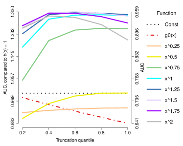
(a) $n=80$, $\ell_{2}$-nn domain

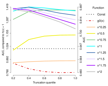
(b) $n=1000$, $\ell_{2}$-nn domain

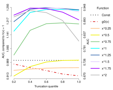
(c) $n=80$, $\ell_{2}^{\complement}$-nn domain

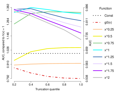
(d) $n=1000$, $\ell_{2}^{\complement}$-nn domain

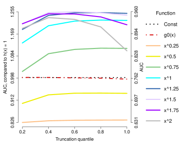
(e) $n=80$, unif-nn domain

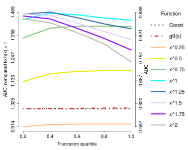
(f) $n=1000$, unif-nn domain

Figure 4: AUCs averaged over 50 trials for support recovery using generalized score matching for log models ($a=0$). Each curve represents either our extension to $g_{0}(\bm{x})$ from Liu and Kanamori (2019) or a choice of power function $h(x)=x^{c}$. The $x$ axes mark the probabilities $\pi$ that determine the truncation points $\bm{C}$ for the truncated component-wise distances. The colors are sorted by the power $c$.

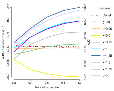
(a) $n=80$, $\ell_{2}$-nn domain

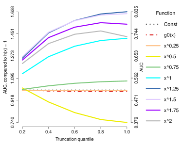
(b) $n=1000$, $\ell_{2}$-nn domain

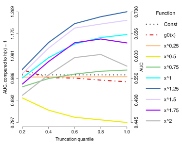
(c) $n=80$, $\ell_{2}^{\complement}$-nn domain

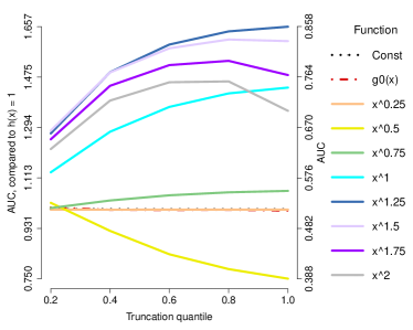
(d) $n=1000$, $\ell_{2}^{\complement}$-nn domain

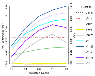
(e) $n=80$, unif-nn domain

(f) $n=1000$, unif-nn domain

Figure 5: AUCs averaged over 50 trials for support recovery using generalized score matching for exponential square-root models ($a=1/2$). Each curve represents either our extension to $g_{0}(\bm{x})$ from Liu and Kanamori (2019) or a choice of power function $h(x)=x^{c}$.

(a) $n=80$, $\ell_{2}$-nn domain

(b) $n=1000$, $\ell_{2}$-nn domain

(c) $n=80$, $\ell_{2}^{\complement}$-nn domain

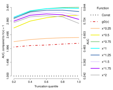
(d) $n=1000$, $\ell_{2}^{\complement}$-nn domain

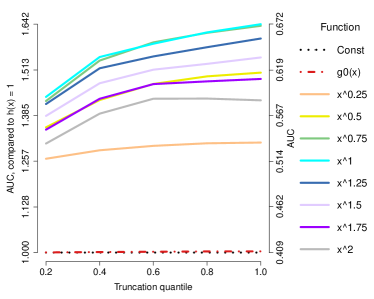
(e) $n=80$, unif-nn domain

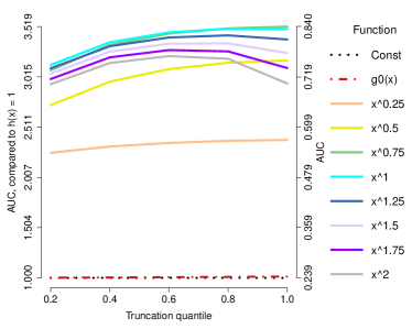
(f) $n=1000$, unif-nn domain

Figure 6: AUCs averaged over 50 trials for support recovery using generalized score matching for Gaussian models ($a=1$) on domains being subsets of $\mathbb{R}_{+}^{m}$. Each curve represents either our extension to $g_{0}(\bm{x})$ from Liu and Kanamori (2019) or a choice of power function $h(x)=x^{c}$.

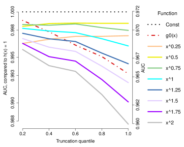
(a) $n=80$, $\ell_{2}$ domain

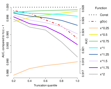
(b) $n=1000$, $\ell_{2}$ domain

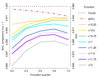
(c) $n=80$, $\ell_{2}^{\complement}$ domain

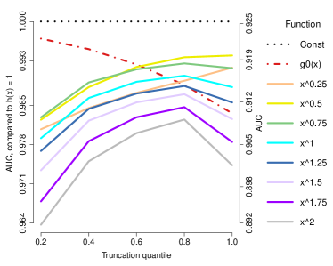
(d) $n=1000$, $\ell_{2}^{\complement}$ domain

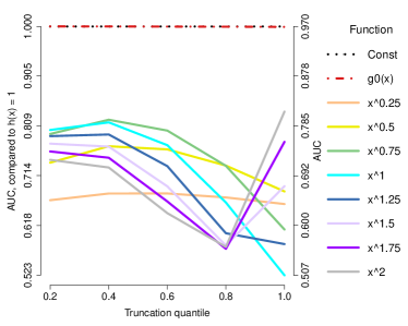
(e) $n=80$, unif domain

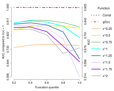
(f) $n=1000$, unif domain

Figure 7: AUCs averaged over 50 trials for support recovery using generalized score matching for Gaussian models ($a=1$) on domains being subsets of $\mathbb{R}^{m}$ (not restricted to $\mathbb{R}_{+}^{m}$). Each curve represents either our extension to $g_{0}(\bm{x})$ from Liu and Kanamori (2019) or a choice of power function $h(x)=x^{c}$.

7 DNA Methylation Networks

We illustrate the use of our generalized score matching for inference of conditional independence relations among DNA methylations based on data for $500$ patients. The dataset contains methylation levels of CpG islands associated with head and neck cancer from The Cancer Genome Atlas (TCGA) (Weinstein et al., 2013). Methylation levels are associated with epigenetic regulation of genes and, according to (Du et al., 2010), are commonly reported as Beta values, a value in $[0,1]$ given by the ratio of the methylated probe intensity and the sum of methylated and unmethylated probe intensities, or M values, defined as the base 2-logit of the Beta values. Supported on $\mathbb{R}$, M values can be analyzed using traditional methods, e.g., via Gaussian graphical models. In contrast, our new methodology allows direct analysis of Beta values using generalized score matching for the $a$-$b$ model framework.

We focus on a subset of CpG sites corresponding to genes known to belong to the pathway for Thyroid cancer according to the Kyoto Encyclopedia of Genes and Genomes (KEGG). Furthermore, we remove sites with clearly bimodal methylations, which we assess using the methods from the R package Mclust. This results in $n=500$ samples and $m=478$ sites belonging to 36 genes.

When considering M values, we estimate the graph encoding the support of the interaction matrix (and hence the conditional dependence structure) in a Gaussian model on $\mathbb{R}^{m}$, i.e., the $a$-$b$ model with $a=b=1$. In doing so, we use the profiled estimator in (24), and choose the upper-bound diagonal multiplier $2-(1+80\sqrt{\log m/n})^{-1}$ as suggested in Section 6.2 of Yu et al. (2019b). The support being all of $\mathbb{R}^{m}$ we simply use the original score matching with $(\bm{h}\circ\bm{\varphi})(\bm{x})=\mathbf{1}_{m}$. For Beta values, we assume a $\log$-$\log$ model ($a=b=0$) on $[0,1]^{m}$, and use the profiled estimator with the upper-bound diagonal multiplier $1+\sqrt{(\tau\log m+\log 4)/(2n)}$ as in (32) with the choice of $\tau=3$. Suggested by our theory, we use $\bm{h}(\bm{x})=\bm{x}^{2}$, and choose the truncation points in $\bm{\varphi}$ to be the 40th sample percentile, as suggested by the simulation results in Figure 4. For our illustration, the $\lambda$ parameter that defines the $\ell_{1}$ penalty on $\mathbf{K}$ is chosen so that the number of edges is equal to 478, the number of sites, following Lin et al. (2016) and Yu et al. (2019b).

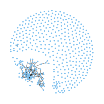
(b) Common edges

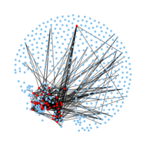
(c) M values

Figure 13: Graphs for CpG sites estimated by regularized generalized score matching estimator using Beta values (a) and M values (c), and their intersection graph (b). Isolated nodes are included and the layout is optimized for the graph for Beta values; red nodes have degree at least 10 (“hub nodes”).

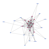
(a) Beta values

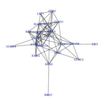
(b) Common edges

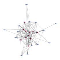
(c) M values

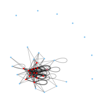
(d) Beta values

(e) Common edges

(f) M values

Figure 14: Graphs in Figure 8 (equivalently Figure 14) aggregated by the genes associated with the CpG sites, with Beta values (a, d) and M values (c, f), and their intersection graph (b, e). Red points indicate genes that are connected to at least 10 other genes in the case of Figure 14

The estimated graphs are presented in Figure 8, where panel (a) is for Beta values, (c) is for M values, and (b) shows their common edges, i.e., the intersection graph. The plots in (a), (b), and (c) exclude isolated nodes and the layout is optimized for each graph. Figure 14 in the appendix includes isolated nodes where the layout is optimized for the graph for Beta values. Figure 14 in the appendix shows the graphs in Figure 8 aggregated by the genes associated with the sites. In (a) and (c), red points indicate nodes with degree at least 10. Sites with the highest node degrees are listed in Table 1, where those shared by the two graphs are highlighted in bold.

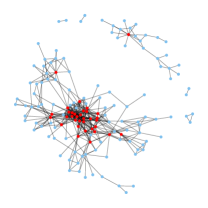
(a) Beta values

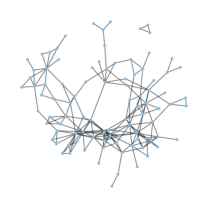
(b) Common edges

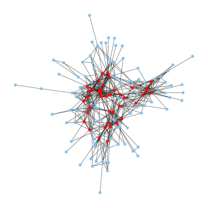
(c) M values

Figure 8: Graphs for CpG sites estimated by regularized generalized score matching estimator using Beta values (a) and M values (c), and their intersection graph (b).

Beta values	M values	Beta values	M values
CDH1—4 (28)	RXRB—24 (25)	LEF1—2 (20)	PAX8—9 (20)
TCF7L1—18 (22)	MAPK3—8 (22)	TCF7L1—13 (20)	TCF7—3 (18)
RXRA—19 (21)	PAX8—6 (21)	CDKN1A—10 (20)	TCF7L1—9 (18)
RXRA—22 (21)	CCND1—19 (20)	CDKN1A—6 (19)	TCF7L1—18 (18)
RET—22 (21)	RXRA—10 (20)	MAPK3—8 (17)	TCF7L2—63 (18)
RXRB—82 (21)	RXRA—19 (20)	PAX8—28 (17)	TPM3—12 (18)
NTRK1—40 (21)	RXRB—18 (20)	PAX8—29 (17)	PAX8—29 (17)

Table 1: List of sites with the highest node degrees in each estimated graph.

We quantify the similarity between the two site graphs (not aggregated) by their Hamming distance and their DeltaCon similarity score (Koutra et al., 2013). The Hamming distance counts the number of edge differences, and thus decreases as two graphs become more similar. Conversely, DeltaCon (Koutra et al., 2013) generates a similarity score in $[0,1]$, and the closer the score is to 1, the more similar the two graphs are.

The Hamming distance between the two graphs is 568, which is considerably smaller than 936, the minimal Hamming distance between the graph for Beta values and 10000 randomly generated graphs with the same number of edges, and 940, that value using the graph for M values. On the other hand, the DeltaCon similarity score between the two original graphs is 0.114, while the maximal score between the Beta graph and 10000 randomly generated graphs is only 0.0781, while that for the M graph is 0.0761. In Figure 9, we compare the distribution of node degrees for both graphs, with interlaced histogram on the left and Q-Q plot on the right. All these results suggest that the two estimated graphs are similar to each other, but that the two analyses also reveal complementary features.

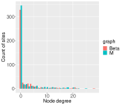
(a) Beta values

(b) Common edges

Figure 9: Interlaced histogram (left) and Q-Q plot (right) showing the node degree distributions for both site graphs.

8 Conclusion

Generalized score matching as proposed in Yu et al. (2019b) is an extension of the method of Hyvärinen (2007) that estimates densities supported on $\mathbb{R}_{+}^{m}$ using a loss, in which the log-gradient of the postulated density, $\nabla\log p(\bm{x})$, is multiplied component-wise with a function $\bm{h}(\bm{x})$. The resulting estimator avoids the often costly calculation of normalizing constants and has a closed-form solution in exponential family models.

In this paper, we further extend generalized score matching to be applicable to more general domains. Specifically, we allow for domains $\mathfrak{D}$ that are component-wise countable union of intervals $\mathfrak{D}$ (see Definition 1). We accomplish this by composing the function $\bm{h}$ with a distance function $\bm{\varphi}_{\bm{C}}=(\varphi_{C_{1},1},\ldots,\varphi_{C_{m},m}):\mathfrak{D}\to\mathbb{R}_{+}^{m}$, where $\varphi_{C_{j},j}(\bm{x})$ is a truncated distance of $x_{j}$ to the boundary of the relevant interval in the section of $\mathfrak{D}$ given by $\bm{x}_{-j}$. The resulting loss can again be approximated by an empirical loss, which is quadratic in the canonical parameters for exponential families.

In our applications we focus on $a$-$b$ pairwise interaction models supported on domains $\mathfrak{D}$ with positive Lebesgue measure. For these models we give a concrete choice of the function $\bm{h}$ and extend the consistency theory for support recovery in Yu et al. (2019b) to Gaussian models on domains that are finite disjoint unions of convex sets, and on bounded domains with positive Lebesgue measure, requiring the sample size to be $n=\Omega(\log m)$. For unbounded domains with $a>0$, we require an additional multiplicative factor that may weakly depend on $m$. Deriving a more explicit requirement on the sample size would be an interesting topic for future work. Finally, in our simulations we adaptively select the truncation points $\bm{C}$ of $\bm{\varphi}_{\bm{C}}$ using the sample quantiles of the untruncated distances. Developing a method to choose the best truncation points remains a topic for further research.

Appendix A Additional Plots

Below we present additional plots for our simulations in Sections 6 and 7.

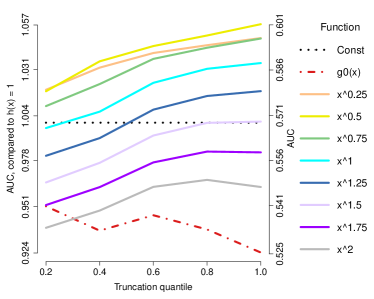
(a) $n=80$, $\ell_{2}$-nn domain

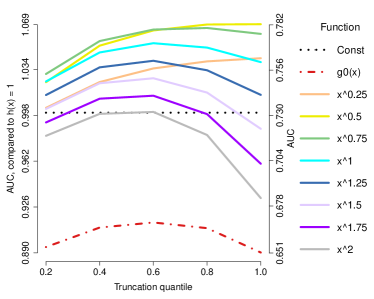
(b) $n=1000$, $\ell_{2}$-nn domain

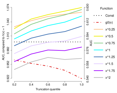
(c) $n=80$, $\ell_{2}^{\complement}$-nn domain

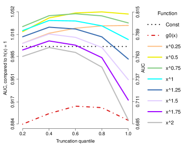
(d) $n=1000$, $\ell_{2}^{\complement}$-nn domain

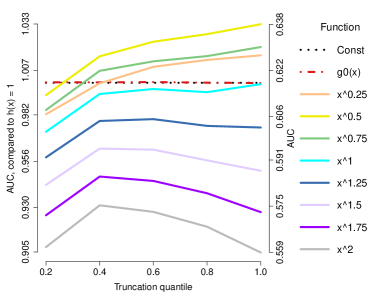
(e) $n=80$, unif-nn domain

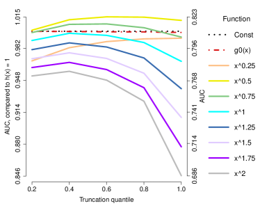
(f) $n=1000$, unif-nn domain

Figure 10: AUCs averaged over 50 trials for support recovery using generalized score matching for the $a=3/2$ models. Each curve represents either our extension to $g_{0}(\bm{x})$ from Liu and Kanamori (2019) or a choice of power function $h(x)=x^{c}$.

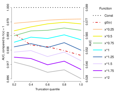
(a) $n=80$, $\ell_{2}$-nn domain

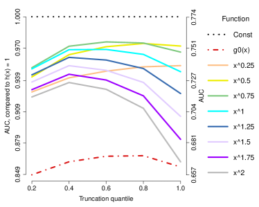
(b) $n=1000$, $\ell_{2}$-nn domain

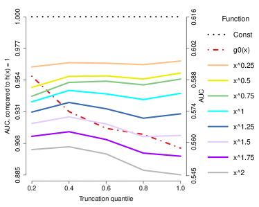
(c) $n=80$, $\ell_{2}^{\complement}$-nn domain

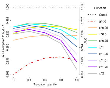
(d) $n=1000$, $\ell_{2}^{\complement}$-nn domain

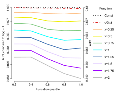
(e) $n=80$, unif-nn domain

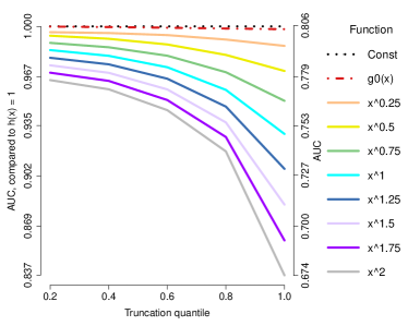
(f) $n=1000$, unif-nn domain

Figure 11: AUCs averaged over 50 trials for support recovery using generalized score matching for the $a=2$ models. Each curve represents either our extension to $g_{0}(\bm{x})$ from Liu and Kanamori (2019) or a choice of power function $h(x)=x^{c}$. The $x$ axes mark the probabilities $\pi$ that determine the truncation points $\bm{C}$ for the truncated component-wise distances. The colors are sorted by the power $c$.

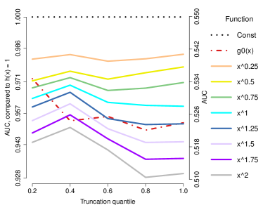
(a) $n=80$, $\ell_{2}$-nn domain

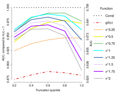
(b) $n=1000$, $\ell_{2}$-nn domain

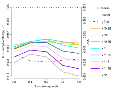
(c) $n=80$, $\ell_{2}^{\complement}$-nn domain

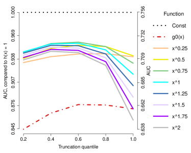
(d) $n=1000$, $\ell_{2}^{\complement}$-nn domain

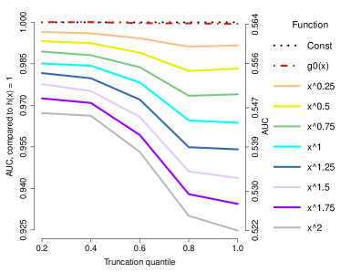
(e) $n=80$, unif-nn domain

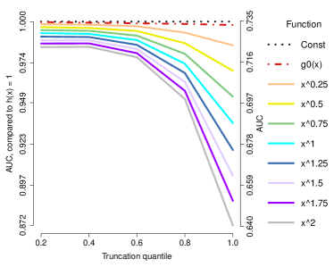
(f) $n=1000$, unif-nn domain

Figure 12: AUCs averaged over 50 trials for support recovery using generalized score matching for the $a=3$ models. Each curve represents either our extension to $g_{0}(\bm{x})$ from Liu and Kanamori (2019) or a choice of power function $h(x)=x^{c}$. The $x$ axes mark the probabilities $\pi$ that determine the truncation points $\bm{C}$ for the truncated component-wise distances. The colors are sorted by the power $c$.

(a) Beta values

Appendix B Proofs

Before proving Lemma 2 we first prove the following lemma.

Lemma 12.

Suppose $h_{1},\ldots,h_{m}$ are absolutely continuous in any bounded sub-interval of $\mathbb{R}_{+}$. Then for any $j=1,\ldots,m$ and any $\bm{x}_{-j}\in\mathfrak{S}_{-j,\mathfrak{D}}$, $(h_{j}\circ\varphi_{j})$ is absolutely continuous in $x_{j}$ in any bounded sub-interval of $\mathfrak{C}_{j,\mathfrak{D}}(\bm{x}_{-j})$.

Proof of Lemma 12.

In the proof we drop the dependency on $\bm{x}_{-j}$ in notation. By assumption, under Equation 7 any bounded sub-interval $[a,b]$ of $\mathfrak{C}_{j,\mathfrak{D}}(\bm{x}_{-j})$ must be a sub-interval of $[a_{k,j},b_{k,j}]$ for some $k$ (for simplicity we do not differentiate among $[a,b]$, $(a,b]$, $[a,b)$ and $(a,b)$ here).

1. If $a_{k,j}>-\infty$ and $b_{k,j}<+\infty$, denote $C_{0}\equiv\min\{C_{j},(b_{k,j}-a_{k,j})/2\}$ and rewrite

   $$\,(h_{j}\circ\varphi_{j})(\bm{x})$$

   $$= \,h_{j}\left(\min(C_{j},x_{j}-a_{k,j},b_{k,j}-x_{j})\right)$$

   $$= \,h_{j}(x_{j}-a_{k,j})\mathds{1}_{x_{j}\in[a_{k,j},a_{k,j}+C_{0}]}+h_{j}(C_{j})\mathds{1}_{x_{j}\in[a_{k,j}+C_{0},b_{k,j}-C_{0}]}+h_{j}(b_{k,j}-x_{j})\mathds{1}_{x_{j}\in[b_{k,j}-C_{0},b_{k,j}]}.$$

   Then by absolute continuity of $h_{j}$ in $[a_{k,j},b_{k,j}]$ it is apparent that $(h_{j}\circ\varphi_{j})$ is differentiable in $x_{j}$ a.e. with partial derivative

   $$h_{j}^{\prime}(x_{j}-a_{k,j})\mathds{1}_{x_{j}\in[a_{k,j},a_{k,j}+C_{0}]}-h_{j}^{\prime}(b_{k,j}-x_{j})\mathds{1}_{x_{j}\in[b_{k,j}-C_{0},b_{k,j}]}.$$

   Then by the absolute continuity of $h_{j}$ again, for $x_{j}\in[a_{k,j},b_{k,j}]$,

   $$\,\int_{a_{k,j}}^{x_{j}}\partial_{j}(h_{j}\circ\varphi_{j})(t_{j};\bm{x}_{-j})\mathop{}\!\mathrm{d}t_{j}$$

   $$= \,h_{j}(x_{j}-a_{k,j})\mathds{1}_{x_{j}\in[a_{k,j},a_{k,j}+C_{0}]}+h_{j}(C_{j})\mathds{1}_{x_{j}\in[a_{k,j}+C_{0},b_{k,j}-C_{0}]}+h_{j}(b_{k,j}-x_{j})\mathds{1}_{x_{j}\in[b_{k,j}-C_{0},b_{k,j}]}$$

   $$= \,(h_{j}\circ\varphi_{j})(\bm{x}),$$

   which proves that $(h_{j}\circ\varphi_{j})(\bm{x})$ is absolutely continuous in $x_{j}$ in $[a_{k,j},b_{k,j}]$, and hence in $[a,b]\subset[a_{k,j},b_{k,j}]$.

2. If $a_{k,j}>-\infty$ and $b_{k,j}=+\infty$, on $[a,b]$ $(h_{j}\circ\varphi_{j})(\bm{x})=h_{j}(\min(C_{j},x_{j}-a_{k,j}))$ is an absolutely continuous function in a linear function of $x_{j}$ truncated above by $C_{j}$, and is thus trivially absolutely continuous in $[a,b]$.

3. If $a_{k,j}=-\infty$ and $b_{k,j}<+\infty$, on $[a,b]$ $(h_{j}\circ\varphi_{j})(\bm{x})=h_{j}(\min(C_{j},b_{k,j}-x_{j}))$ is an absolutely continuous function in a linear function of $x_{j}$ truncated above by $C_{j}$, and is thus trivially absolutely continuous in $[a,b]$.

4. If $a_{k,j}=-\infty$ and $b_{k,j}=+\infty$, $(h_{j}\circ\varphi_{j})(\bm{x})=h_{j}(C_{j})$ is constant and hence trivially absolutely continuous in $[a,b]$.

∎

Proof of Lemma 2.

By simple manipulation

$$J_{\bm{h},\bm{C},\mathfrak{D}}(p) \equiv\frac{1}{2}\int_{\mathfrak{D}}p_{0}(\bm{x})\left\|\nabla\log p(\bm{x})\odot\left(\bm{h}\circ\bm{\varphi}\right)^{1/2}(\bm{x})-\nabla\log p_{0}(\bm{x})\odot\left(\bm{h}\circ\bm{\varphi}\right)^{1/2}(\bm{x})\right\|_{2}^{2}\mathop{}\!\mathrm{d}\bm{x}$$ (33)

$$=\frac{1}{2}\sum_{j=1}^{m}\int_{\mathfrak{D}}p_{0}(\bm{x})(h_{j}\circ\varphi_{j})(\bm{x})\left(\partial_{j}\log p_{0}(\bm{x})-\partial_{j}\log p(\bm{x})\right)^{2}\mathop{}\!\mathrm{d}\bm{x}$$

$$=\frac{1}{2}\sum_{j=1}^{m}\int_{\mathfrak{D}}p_{0}(\bm{x})(h_{j}\circ\varphi_{j})(\bm{x})\left(\partial_{j}\log p(\bm{x})\right)^{2}\mathop{}\!\mathrm{d}\bm{x}$$

$$-\sum_{j=1}^{m}\int_{\mathfrak{D}}p_{0}(\bm{x})(h_{j}\circ\varphi_{j})(\bm{x})\partial_{j}\log p_{0}(\bm{x})\partial_{j}\log p(\bm{x})\mathop{}\!\mathrm{d}\bm{x}+\mathrm{const}.$$ (34)

By (34) it suffices to prove for all $j=1,\dots,m$ that

$$\int_{\mathfrak{D}}p_{0}(\bm{x})(h_{j}\circ\varphi_{j})(\bm{x})\partial_{j}\log p_{0}(\bm{x})\partial_{j}\log p(\bm{x})\mathop{}\!\mathrm{d}\bm{x}=-\int_{\mathfrak{D}}p_{0}(\bm{x})\partial_{j}\left[(h_{j}\circ\varphi_{j})(\bm{x})\partial_{j}\log p(\bm{x})\right]\mathop{}\!\mathrm{d}\bm{x}.$$ (35)

Since $\int_{\mathfrak{D}}p_{0}(\bm{x})\left\|\nabla\log p(\bm{x})\odot(\bm{h}\circ\bm{\varphi})^{1/2}(\bm{x})\right\|_{2}^{2}\mathop{}\!\mathrm{d}\bm{x}$ and $\int_{\mathfrak{D}}p_{0}(\bm{x})\left\|\nabla\log p_{0}(\bm{x})\odot(\bm{h}\circ\bm{\varphi})^{1/2}(\bm{x})\right\|_{2}^{2}\mathop{}\!\mathrm{d}\bm{x}$ are both finite under assumption, by $|2ab|\leq a^{2}+b^{2}$ the integrand in the left-hand side of (35) is integrable. Then by Fubini-Tonelli

$$\,\int_{\mathfrak{D}}p_{0}(\bm{x})(h_{j}\circ\varphi_{j})(\bm{x})\partial_{j}\log p_{0}(\bm{x})\partial_{j}\log p(\bm{x})\mathop{}\!\mathrm{d}\bm{x}$$

$$= \,\int_{\mathfrak{S}_{-j}}\int_{\mathfrak{C}_{j}(\bm{x}_{-j})}\underbrace{(h_{j}\circ\varphi_{j})(\bm{x})\partial_{j}p_{0}(\bm{x})\partial_{j}\log p(\bm{x})}_{\equiv f(\bm{x})}\mathop{}\!\mathrm{d}x_{j}\mathop{}\!\mathrm{d}\bm{x}_{-j}$$

$$= \,\int_{\mathfrak{S}_{-j}}\int_{\mathbb{R}}\mathds{1}_{\mathfrak{C}_{j}(\bm{x}_{-j})}(x_{j})f(\bm{x})\mathop{}\!\mathrm{d}x_{j}\mathop{}\!\mathrm{d}\bm{x}_{-j}$$

$$= \,\int_{\mathfrak{S}_{-j}}\int_{\mathbb{R}}\left[\sum_{k=1}^{K_{j}(\bm{x}_{-j})}\mathds{1}_{[a_{k,j}(\bm{x}_{-j}),\,b_{k,j}(\bm{x}_{-j})]}(x_{j})\right]f(x_{j};\bm{x}_{-j})\mathop{}\!\mathrm{d}x_{j}\mathop{}\!\mathrm{d}\bm{x}_{-j}$$

$$= \,\int_{\mathfrak{S}_{-j}}\left[\sum_{k=1}^{K_{j}(\bm{x}_{-j})}\int_{a_{k,j}(\bm{x}_{-j})}^{b_{k,j}(\bm{x}_{-j})}f(x_{j};\bm{x}_{-j})\mathop{}\!\mathrm{d}x_{j}\right]\mathop{}\!\mathrm{d}\bm{x}_{-j}$$ (36)

where the interchangeability of integration and (potentially infinite) summation is justified by Fubini-Tonelli again. Then using the decomposition of the domain in (7) while omitting the dependency of $a_{k,j}$ and $b_{k,j}$ on $\bm{x}_{-j}$ in notation, for a.e. $\bm{x}_{-j}\in\mathfrak{S}_{-j}$ and any $k=1,\ldots,K_{j}(\bm{x}_{-j})$ we have

$$\,\int_{a_{k,j}}^{b_{k,j}}f(\bm{x})\mathop{}\!\mathrm{d}x_{j}$$

$$= \,\int_{a_{k,j}}^{b_{k,j}}(h_{j}\circ\varphi_{j})(\bm{x})\partial_{j}p_{0}(\bm{x})\partial_{j}\log p(\bm{x})\mathop{}\!\mathrm{d}x_{j}$$

$$= \,\lim_{x_{j}\nearrow b_{k_{j}}^{-}}(h_{j}\circ\varphi_{j})(\bm{x})p_{0}(\bm{x})\partial_{j}\log p(\bm{x})-\lim_{x_{j}\searrow a_{k_{j}}^{+}}(h_{j}\circ\varphi_{j})(\bm{x})p_{0}(\bm{x})\partial_{j}\log p(\bm{x})$$

$$-\int_{a_{k,j}}^{b_{k,j}}p_{0}(\bm{x})\partial_{j}\left[(h_{j}\circ\varphi_{j})(\bm{x})\partial_{j}\log p(\bm{x})\right]\mathop{}\!\mathrm{d}x_{j}$$

$$= \,-\int_{a_{k,j}}^{b_{k,j}}p_{0}(\bm{x})\partial_{j}\left[(h_{j}\circ\varphi_{j})(\bm{x})\partial_{j}\log p(\bm{x})\right]\mathop{}\!\mathrm{d}x_{j},$$

by integration by parts and by Assumption (A1) on the limits going to 0. The integration by parts is justified by the fundamental theorem of calculus for absolutely continuous functions (Lemma 12) as well as the product rule (cf. proof of Lemma 19 in Yu et al. (2019b)). Thus, by going backwards using Fubini-Tonelli twice again, (36) becomes

$$\,\int_{\mathfrak{S}_{-j}}\left\{-\sum_{k=1}^{K_{j}(\bm{x}_{-j})}\int_{a_{k,j}(\bm{x}_{-j})}^{b_{k,j}(\bm{x}_{-j})}p_{0}(\bm{x})\partial_{j}\left[(h_{j}\circ\varphi_{j})(\bm{x})\partial_{j}\log p(\bm{x})\right]\mathop{}\!\mathrm{d}x_{j}\right\}\mathop{}\!\mathrm{d}\bm{x}_{-j}$$

$$= \,-\int_{\mathfrak{S}_{-j}}\int_{\mathfrak{C}_{j}(\bm{x}_{-j})}p_{0}(\bm{x})\partial_{j}\left[(h_{j}\circ\varphi_{j})(\bm{x})\partial_{j}\log p(\bm{x})\right]\mathop{}\!\mathrm{d}x_{j}\mathop{}\!\mathrm{d}\bm{x}_{-j}$$

$$= \,-\int_{\mathfrak{D}}p_{0}(\bm{x})\partial_{j}\left[(h_{j}\circ\varphi_{j})(\bm{x})\partial_{j}\log p(\bm{x})\right]\mathop{}\!\mathrm{d}\bm{x},$$

proving (35). ∎

Proof of Theorem 5.

Note that the condition ${\bm{v}^{a}}^{\top}\mathbf{K}\bm{v}^{a}>0$ $\forall\bm{v}\in\mathfrak{D}\backslash\{\bm{0}\}$ implies that ${\bm{v}^{a}}^{\top}\mathbf{K}\bm{v}^{a}>0$ $\forall\bm{v}\in\mathfrak{D}_{+}\equiv\{\bm{v}/\|\bm{v}\|_{2}:\bm{v}\in\mathfrak{D}\backslash\{\bm{0}\}\}\subseteq\{\bm{v}\in\mathbb{R}^{m}:\|\bm{v}\|_{2}=1\}\equiv\mathbb{S}^{m-1}$ with $\mathbb{S}^{m-1}$ compact, so

$$N_{\mathbf{K}} \equiv\inf_{\bm{v}\in\mathfrak{D}\backslash\{\bm{0}\}}{\bm{v}^{a}}^{\top}\mathbf{K}\bm{v}^{a}/{\bm{v}^{a}}^{\top}\bm{v}^{a}=\inf_{\bm{v}\in\mathfrak{D}_{+}}{\bm{v}^{a}}^{\top}\mathbf{K}\bm{v}^{a}/{\bm{v}^{a}}^{\top}\bm{v}^{a}$$

$$\geq\inf_{\bm{v}\in\mathbb{S}^{m-1}}{\bm{v}^{a}}^{\top}\mathbf{K}\bm{v}^{a}/{\bm{v}^{a}}^{\top}\bm{v}^{a}>0.$$

(1) Case $a>0$ and $b>0$ (CC1, CC2): Since $p$ is bounded everywhere, it is integrable over a bounded $\mathfrak{D}$ (proving (CC1)). Otherwise, assume $\mathfrak{D}$ is unbounded. If either $a$ or $b$ is non-integer, then $\mathfrak{D}\subset\mathbb{R}_{+}^{m}$ and a sufficient condition is $\bm{v}^{a}\mathbf{K}\bm{v}^{a}>0$ $\forall\bm{v}\in\mathfrak{D}\backslash\{\bm{0}\}$, and either $\bm{\eta}^{\top}\bm{v}^{b}\leq 0$ $\forall\bm{v}\in\mathfrak{D}$ or $2a>b>0$, corresponding to (i) and (ii) in the Proof of Theorem 9 in Section A.3 of Yu et al. (2019b), respectively. If $a$ and $b$ are both integers, $\mathfrak{D}\subset\mathbb{R}^{m}$ and the same sufficient condition can be implied following the same proof in Yu et al. (2019b), with integration over $(-\infty,+\infty)$ instead of $(0,+\infty)$. This proves (CC2).

(2) Case $a>0$ and $b=0$ (CC3): By definition $\mathfrak{D}\subseteq\mathbb{R}_{+}^{m}$. If $\mathfrak{D}$ is bounded, $-\frac{1}{2a}{\bm{x}^{a}}^{\top}\mathbf{K}\bm{x}^{a}$ as a continuous function is bounded, and so it suffices to bound $\int_{\mathfrak{D}}\exp\left(\bm{\eta}^{\top}\log(\bm{x})\right)\mathop{}\!\mathrm{d}\bm{x}=\int_{\mathfrak{D}}\prod_{j=1}^{m}x_{j}^{\eta_{j}}\mathop{}\!\mathrm{d}\bm{x}\leq\prod_{j=1}^{m}\int_{\rho_{j}(\mathfrak{D})}x_{j}^{\eta_{j}}\mathop{}\!\mathrm{d}x_{j}<+\infty$ if $\eta_{j}>-1$ for all $j$ such that $0\in\rho_{j}(\mathfrak{D})$, where for the $\leq$ step we used the fact that $x_{j}>0$. This proves (CC3) (i).

If $\mathfrak{D}$ is unbounded and ${\bm{v}^{a}}^{\top}\mathbf{K}\bm{v}^{a}>0$ for all $\bm{v}\in\mathfrak{D}\backslash\{\bm{0}\}$, using the fact that $\exp(\cdots)>0$,

$$\int_{\mathfrak{D}}p_{\bm{\eta},\mathbf{K}}(\bm{x})\mathop{}\!\mathrm{d}\bm{x} =\int_{\mathfrak{D}}\exp\left(-{\bm{x}^{a}}^{\top}\mathbf{K}\bm{x}^{a}/(2a)+\bm{\eta}^{\top}\log(\bm{x})\right)\mathop{}\!\mathrm{d}\bm{x}$$

$$\leq\prod_{j=1}^{m}\int_{\rho_{j}(\mathfrak{D})}\exp\left(-N_{\mathbf{K}}x_{j}^{2a}/(2a)+\eta_{j}\log(x_{j})\right)\mathop{}\!\mathrm{d}x_{j}.$$

Note that the indefinite integral of the last display is

$$-\frac{1}{2a}x^{1+\eta_{j}}\left(\frac{N_{\mathbf{K}}}{2a}x^{2a}\right)^{-(1+\eta_{j})/(2a)}\Gamma\left[\frac{1+\eta_{j}}{2a},\frac{N_{\mathbf{K}}x^{2a}}{2a}\right]$$

so the definite integral is finite if and only if $\eta_{j}>-1$ for all $j$ s.t. $0\in\rho_{j}(\mathfrak{D})$. This proves (CC3) (ii).

If $\mathfrak{D}$ is unbounded and ${\bm{v}^{a}}^{\top}\mathbf{K}\bm{v}^{a}\geq 0$ for all $\bm{v}\in\mathfrak{D}$, then $\int_{\mathfrak{D}}p_{\bm{\eta},\mathbf{K}}(\bm{x})\mathop{}\!\mathrm{d}\bm{x}\leq\prod_{j=1}^{m}\int_{\rho_{j}(\mathfrak{D})}x_{j}^{\eta_{j}}\mathop{}\!\mathrm{d}x_{j}<\infty$ if $\eta_{j}>-1$ for all $j$ s.t. $0\in\rho_{j}(\mathfrak{D})$ and $\eta_{j}<-1$ for all $j$ s.t. $\rho_{j}(\mathfrak{D})$ is unbounded. This proves (CC3) (iii).

(3) Case $a=0$, $\mathfrak{D}$ is bounded and $0\not\in\rho_{j}(\mathfrak{D})$ for all $j$ (CC4): If $\mathfrak{D}$ is bounded and $0\not\in\rho_{j}(\mathfrak{D})$ for all $j$, then $\log(\mathfrak{D})$ is bounded, and since the integrand is continuous and bounded, the integral is finite without any further requirements.

(4) Case $a=0$ and $b=0$ (CC5): Assume $\log(\bm{x})^{\top}\mathbf{K}\log(\bm{x})>0$ for all $\bm{x}\in\mathfrak{D}$, then

$$\int_{\mathfrak{D}}p_{\bm{\eta},\mathbf{K}}(\bm{x})\mathop{}\!\mathrm{d}\bm{x}= \int_{\mathfrak{D}}\exp\left(-\frac{1}{2}{\log(\bm{x})}^{\top}\mathbf{K}\log(\bm{x})+\bm{\eta}^{\top}\log(\bm{x})\right)\mathop{}\!\mathrm{d}\bm{x}$$

$$= \int_{\log(\mathfrak{D})}\exp\left(-\frac{1}{2}{\bm{x}}^{\top}\mathbf{K}\bm{x}+(\bm{\eta}+\mathbf{1}_{m})^{\top}\bm{x}\right)\mathop{}\!\mathrm{d}\bm{x}$$

$$< \prod_{j=1}^{m}\int_{\log(\rho_{j}(\mathfrak{D}))}\exp\left(-N_{\mathbf{K}}x_{j}^{2}/2+(\eta_{j}+1)x_{j}\right)\mathop{}\!\mathrm{d}x_{j}$$

$$< \prod_{j=1}^{m}\int_{-\infty}^{\infty}\exp\left(-N_{\mathbf{K}}x_{j}^{2}/2+(\eta_{j}+1)x_{j}\right)\mathop{}\!\mathrm{d}x_{j}<+\infty$$

since the integrand is proportional to a univariate Gaussian density.

(5) Case $a=0$ and $b>0$ (CC6, CC7): Assume $\log(\bm{x})^{\top}\mathbf{K}\log(\bm{x})>0$ for all $\bm{x}\in\mathfrak{D}$ and $\eta_{j}\leq 0$ for all $j$ s.t. $\rho_{j}(\mathfrak{D})$ is unbounded (from above). Then

$$\int_{\mathfrak{D}}p_{\bm{\eta},\mathbf{K}}(\bm{x})\mathop{}\!\mathrm{d}\bm{x}= \int_{\mathfrak{D}}\exp\left(-\frac{1}{2}{\log(\bm{x})}^{\top}\mathbf{K}\log(\bm{x})+\bm{\eta}^{\top}\bm{x}^{b}\right)\mathop{}\!\mathrm{d}\bm{x}$$

$$= \int_{\log(\mathfrak{D})}\exp\left(-\frac{1}{2}\bm{x}^{\top}\mathbf{K}\bm{x}+\mathbf{1}_{m}^{\top}\bm{x}+\bm{\eta}^{\top}\exp(b\bm{x})\right)\mathop{}\!\mathrm{d}\bm{x}$$

$$< \prod_{j=1}^{m}\int_{\log(\rho_{j}(\mathfrak{D}))}\exp\left(-N_{\mathbf{K}}x_{j}^{2}/2+x_{j}+\eta_{j}\exp(bx_{j})\right)\mathop{}\!\mathrm{d}x_{j}$$

$$\leq \prod_{j=1}^{m}\int_{-\infty}^{\infty}c_{j}\exp\left(-N_{\mathbf{K}}x_{j}^{2}/2+x_{j}\right)\mathop{}\!\mathrm{d}x_{j}<+\infty,$$

where $c_{j}\equiv 1$ if $\eta_{j}\leq 0$ or $c_{j}\equiv\exp\left(\eta_{j}\left(\sup\rho_{j}(\mathfrak{D})\right)^{b}\right)>+\infty$ otherwise. This proves (CC6).

Finally, if $\log(\mathfrak{D})$ is unbounded and $\log(\bm{x})^{\top}\mathbf{K}\log(\bm{x})\geq 0$ for all $\bm{x}\in\mathfrak{D}$, the integral is bounded by

$$\prod_{j=1}^{m}\int_{\log(\rho_{j}(\mathfrak{D}))}\exp\left(x_{j}+\eta_{j}\exp(bx_{j})\right)\mathop{}\!\mathrm{d}x_{j}$$

which is finite if and only if $\eta_{j}<0$ for all $j$ s.t. $\rho_{j}(\mathfrak{D})$ is unbounded (from above). This proves (CC7).

∎

Proof of Theorem 7.

It suffices to consider the case $\mathfrak{D}=\mathbb{R}_{+}^{m}$ for general $a$ and $b$ as well as $\mathfrak{D}=\mathbb{R}^{m}$ for integer $a>0$ and $b>0$ (so that (20) is well defined on $\mathbb{R}^{m}$): For (A.1), the irregularities only occur at the boundary points, but with the composition $(h_{j}\circ\varphi_{j})(\bm{x})$ with $x_{j}$ approaching any finite boundary point behaves like $h_{j}(x_{j})$ with $x_{j}\searrow 0^{+}$ in $\mathfrak{D}=\mathbb{R}_{+}^{m}$, and $(h_{j}\circ\varphi_{j})(\bm{x})$ with $x_{j}\to\infty$ behaves like $h_{j}(x_{j})$ with $x_{j}\to\infty$ in $\mathfrak{D}=\mathbb{R}_{+}^{m}$ (or $\mathbb{R}^{m}$ if applicable). For (A.2), obviously integrability over $\mathfrak{D}$ follows from that over $\mathfrak{D}=\mathbb{R}_{+}^{m}$ or $\mathbb{R}^{m}$. (A.3) is trivially satisfied by a power function $h_{j}$.

As in the proof of Theorem 5, $N_{\mathbf{K}}\equiv\inf_{\bm{v}\in\mathfrak{D}}{\bm{v}^{a}}^{\top}\mathbf{K}\bm{v}^{a}/{\bm{v}^{a}}^{\top}\bm{v}^{a}>0$.

(1) The case for $a>0$ and $b\geq 0$ and $\mathfrak{D}=\mathbb{R}_{+}^{m}$ is covered in Yu et al. (2019b). The proof for the case for $a>0$ and $b>0$ and $\mathfrak{D}=\mathbb{R}^{m}$ is analogous and omitted.

(2) Case $a=0$ and $b=0$:

$$\,\left|p_{0}(\bm{x})\partial_{j}\log p(\bm{x})\right|$$

$$\propto \,\exp\left(-\frac{1}{2}\log(\bm{x})^{\top}\mathbf{K}_{0}\log(\bm{x})+\bm{\eta}_{0}^{\top}\log(\bm{x})\right)$$

$$\times\left|x_{j}^{-1}\left(\eta_{j}-\bm{\kappa}_{j,-j}^{\top}\log(\bm{x}_{-j})\right)-\kappa_{jj}x_{j}^{-1}\log x_{j}\right|$$

$$\leq \,\Big{|}\left(\eta_{j}-\bm{\kappa}_{j,-j}^{\top}\log\bm{x}_{-j}\right)\exp\left[-N_{\mathbf{K}_{0}}(\log x_{j})^{2}/2+(\eta_{j}-1)\log x_{j}\right]$$

$$-\kappa_{jj}\exp\left[-N_{\mathbf{K}_{0}}(\log x_{j})^{2}/2+(\eta_{j}-1)\log x_{j}\right]\log x_{j}\Big{|}$$

$$\times\prod_{k\neq m}\exp\left(-N_{\mathbf{K}_{0}}(\log x_{k})^{2}/2+\eta_{j}\log x_{k}\right)$$

$$\propto \,\mathcal{O}\left[\exp\left(-N_{\mathbf{K}_{0}}y_{j}^{2}/2+(\eta_{j}-1)y_{j}\right)\right]+\mathcal{O}\left[\exp\left(-N_{\mathbf{K}_{0}}y_{j}^{2}/2+(\eta_{j}-1)y_{j}\right)y_{j}\right]$$

which apparently vanishes as $x_{j}\searrow 0^{+}$ and $x_{j}\nearrow+\infty$ with $y_{j}\equiv\log(x_{j})$ since it is dominated by a constant times a Gaussian density in $y_{j}$. Thus, by Proposition 3, (A.1) is satisfied with any $\alpha_{j}\geq 0$. Likewise, for (A.2),

$$\,\int_{\mathbb{R}_{+}^{m}}p_{0}(\bm{x})\left\|\nabla\log p(\bm{x})\odot(\bm{h}\circ\bm{\varphi})^{1/2}(\bm{x})\right\|_{2}^{2}\mathop{}\!\mathrm{d}\bm{x}$$

$$\leq \,\mathrm{const}\cdot\sum_{j=1}^{m}\int_{\mathbb{R}_{+}^{m}}\prod_{k=1}^{m}\exp\left[-N_{\mathbf{K}_{0}}(\log x_{k})^{2}/2+\eta_{k}\log(x_{k})\right]\times$$

$$\quad\quad\quad\quad h_{j}(x_{j})\left[x_{j}^{-1}\left(\eta_{j}-\bm{\kappa}_{j,-j}^{\top}\log(\bm{x}_{-j})\right)-\kappa_{jj}x_{j}^{-1}\log x_{j}\right]^{2}\mathop{}\!\mathrm{d}\bm{x},$$

which can be decomposed into a sum of products of univariate integrals of the form

$$\mathrm{const}\cdot\exp\left(-N_{\mathbf{K}_{0}}(\log x_{j})^{2}/2+A\log(x_{j})\right)(\log x_{j})^{B}(h_{j}(x_{j}))^{C}$$

with $B=0,1,2$, $C=0,1$, and constants $A$. With $h_{j}(x_{j})=x_{j}^{\alpha_{j}}$ for any $\alpha_{j}\geq 0$ this is bounded by some Gaussian density in $\log x_{j}$, so $\int_{\mathbb{R}_{+}^{m}}p_{0}(\bm{x})\|\nabla\log p(\bm{x})\odot(\bm{h}\circ\bm{\varphi})^{1/2}(\bm{x})\|_{2}^{2}\mathop{}\!\mathrm{d}\bm{x}<+\infty$. Similarly, we have $\int_{\mathbb{R}_{+}^{m}}p_{0}(\bm{x})\|[\nabla\log p(\bm{x})\odot(\bm{h}\circ\bm{\varphi})(\bm{x})]^{\prime}\|_{1}\mathop{}\!\mathrm{d}\bm{x}<+\infty$ and the proof is omitted.

(3) Case $a=0$ and $b>0$: Recall $\rho_{j}(\mathfrak{D})\equiv\overline{\{x_{j}:\bm{x}\in\mathfrak{D}\}}$. Let $\rho_{j}^{*}(\mathfrak{D})\equiv\sup\rho_{j}(\mathfrak{D})$. Since we assume that $\eta_{j}\leq 0$ for any $j$ such that $\rho_{j}^{*}(\mathfrak{D})<+\infty$,

$$\,p_{0}(\bm{x})\partial_{j}\log p(\bm{x})$$

$$\propto \,\exp\left(-\frac{1}{2}\log(\bm{x})^{\top}\mathbf{K}_{0}\log(\bm{x})+\frac{1}{b}\bm{\eta}_{0}^{\top}\bm{x}^{b}\right)$$

$$\times\left[\eta_{j}x_{j}^{b-1}-x_{j}^{-1}\bm{\kappa}_{j,-j}^{\top}\log(\bm{x}_{-j})-\kappa_{jj}x_{j}^{-1}\log x_{j}\right]$$

$$\leq \,\exp\left(-\frac{1}{2}\log(\bm{x})^{\top}\mathbf{K}_{0}\log(\bm{x})+\frac{1}{b}\sum_{j:\rho_{j}^{*}(\mathfrak{D})<+\infty}\eta_{0j}(\rho_{j}^{*}(\mathfrak{D}))^{b}\right)$$

$$\times\left[-x_{j}^{-1}\bm{\kappa}_{j,-j}^{\top}\log(\bm{x}_{-j})-\kappa_{jj}x_{j}^{-1}\log x_{j}\right]$$

$$\propto \,\exp\left(-\frac{1}{2}\log(\bm{x})^{\top}\mathbf{K}_{0}\log(\bm{x})\right)\left[-x_{j}^{-1}\bm{\kappa}_{j,-j}^{\top}\log(\bm{x}_{-j})-\kappa_{jj}x_{j}^{-1}\log x_{j}\right]$$

is bounded by the corresponding quantity in the $a=b=0$ case with $\bm{\eta}=\bm{0}_{m}$, and (A.1) is thus satisfied. Similarly, the two quantities for (A.2) are bounded by a constant times those in the $a=b=0$ case with $\bm{\eta}=\bm{0}_{m}$ and (A.2) is thus also satisfied. ∎

Proof of Theorem 9.

It suffices to bound $\bm{\Gamma}$ and $\bm{g}$ using their forms in Section 4.3 and apply Theorem 1 in Lin et al. (2016). Thus, we first find the bounds of $(h_{j}\circ\varphi_{j})(\bm{x})x_{j}^{p_{j}}x_{k}^{p_{k}}x_{\ell}^{p_{\ell}}$ with $h_{j}(x)=x^{\alpha_{j}}$, $\alpha_{j}\geq 0$, $\alpha_{j}\geq-p_{j}$, $p_{j}\in\mathbb{R}$, $p_{k}\geq 0$, $p_{\ell}\geq 0$ and $x_{i}\in[u_{i},v_{i}]$ for $i=1,\ldots,m$. Suppose without loss of generality that $j$, $k$, $\ell$ are all different, as

$$\max_{x_{j}}f_{j,1}(x_{j})\max_{x_{j}}f_{j,2}(x_{j})\max_{x_{j}}f_{j,3}(x_{j})\geq\max_{x_{j}}\left(f_{j,1}(x_{j})f_{j,2}(x_{j})f_{j,3}(x_{j})\right)\geq 0$$

for any nonnegative functions $f_{j,1}$, $f_{j,2}$, $f_{j,3}$.

As $x_{j}$ approaches its boundary, $\varphi_{j}(\bm{x})\searrow 0^{+}$ and hence $(h_{j}\circ\varphi_{j})(\bm{x})x_{j}^{p_{j}}\searrow 0^{+}$ if $\alpha_{j}>-p_{j}$. The lower bound 0 for $(h_{j}\circ\varphi_{j})(\bm{x})x_{j}^{p_{j}}x_{k}^{p_{k}}x_{\ell}^{p_{\ell}}$ is thus tight enough.

As for the upper bound, the only way for the quantity to be unbounded from above is when $x_{j}\searrow 0^{+}$ and $p_{j}<0$, but as $x_{j}\searrow 0^{+}$, $(h_{j}\circ\varphi_{j})(\bm{x})=x_{j}^{\alpha_{j}}$ so this cannot happen with the choice of $\alpha_{j}\geq-p_{j}$. Noting that $h_{j}$ is monotonically increasing, we consider the following cases:

1. Suppose $x_{j}\geq(u_{j}+v_{j})/2$. Then

   $$(h_{j}\circ\varphi_{j})(\bm{x}) \leq h_{j}\left(\min\left\{C_{j},v_{j}-x_{j}\right\}\right)$$

   $$\leq h_{j}(\min\{C_{j},(v_{j}-u_{j})/2\})$$

   $$\leq\min\{C_{j}^{\alpha_{j}},(v_{j}-u_{j})^{\alpha_{j}}/2^{\alpha_{j}}\},$$

   and $x_{j}^{p_{j}}\leq(u_{j}+v_{j})^{p_{j}}/2^{p_{j}}$ if $p_{j}<0$ or $x_{j}^{p_{j}}\leq v_{j}^{p_{j}}$ if $p_{j}\geq 0$.

2. Suppose $x_{j}\leq(u_{j}+v_{j})/2$. Then

   $$(h_{j}\circ\varphi_{j})(\bm{x})x_{j}^{p_{j}} \leq h_{j}\left(\min\left\{C_{j},x_{j}-u_{j}\right\}\right)x_{j}^{p_{j}}$$

   $$=\min\{C_{j}^{\alpha_{j}},(x_{j}-u_{j})^{\alpha_{j}}\}x_{j}^{p_{j}}.$$

   Now let $f(x)=(\min\{C_{j},x-u_{j}\})^{\alpha_{j}}x^{p_{j}}$. Then $(\log f(x))^{\prime}=\alpha_{j}/(x-u_{j})\mathds{1}_{x<u_{j}+C_{j}}+p_{j}/x$. For $x\geq u_{j}+C_{j}$ this has the same sign as $p_{j}$, otherwise it is equal to $((\alpha_{j}+p_{j})x-u_{j}p_{j})/(x(x-u_{j}))\geq 0$ on $(u_{j},v_{j})$ since $x>u_{j}$, $\alpha_{j}\geq-p_{j}$ and $\alpha_{j}\geq 0$. This implies that if $p_{j}\geq 0$ or $v_{j}-u_{j}\leq 2C_{j}$, $f$ is increasing on $(u_{j},(u_{j}+v_{j})/2)$, and so $(h_{j}\circ\varphi_{j})(\bm{x})x_{j}^{p_{j}}\leq\min\left\{C_{j},(v_{j}-u_{j})/2\right\}^{\alpha_{j}}(u_{j}+v_{j})^{p_{j}}/2^{p_{j}}$; otherwise, $f$ is increasing on $(u_{j},u_{j}+C_{j})$ and decreasing on $(u_{j}+C_{j},(u_{j}+v_{j})/2)$, so $(h_{j}\circ\varphi_{j})(\bm{x})x_{j}^{p_{j}}\leq C_{j}^{\alpha_{j}}(u_{j}+C_{j})^{p_{j}}$.

Thus, defining

$$\,\zeta_{j}(\alpha_{j},p_{j})$$

$$\equiv \,\begin{cases}\min\left\{C_{j},(v_{j}-u_{j})/2\right\}^{\alpha_{j}}(u_{j}+v_{j})^{p_{j}}/2^{p_{j}},&p_{j}<0,v_{j}-u_{j}\leq 2C_{j},\\ \min\left\{C_{j},(v_{j}-u_{j})/2\right\}^{\alpha_{j}}(u_{j}+C_{j})^{p_{j}},&p_{j}<0,v_{j}-u_{j}>2C_{j},\\ \min\left\{C_{j},(v_{j}-u_{j})/2\right\}^{\alpha_{j}}v_{j}^{p_{j}},&p_{j}\geq 0,\end{cases}\$$

we have $0\leq(h_{j}\circ\varphi_{j})(\bm{x})x_{j}^{p_{j}}x_{k}^{p_{k}}x_{\ell}^{p_{\ell}}\leq\zeta_{j}(\alpha_{j},p_{j})v_{k}^{p_{k}}v_{\ell}^{p_{\ell}}$. Now assume additionally that $\alpha_{j}\geq\max\{1,1-p_{j}\}$, then by $h_{j}^{\prime}(x)=\alpha_{j}x_{j}^{\alpha_{j}-1}$, $0\leq\partial_{j}(h_{j}\circ\varphi_{j})(\bm{x})x_{j}^{p_{j}}x_{k}^{p_{k}}\leq\alpha_{j}\zeta_{j}(\alpha_{j}-1,p_{j})v_{k}^{p_{k}}$.

First assume $a>0$. Then assuming $\alpha_{1},\ldots,\alpha_{m}\geq\max\{1,2-2a,2-2b,1-a,2-a,2-b\}=\max\{1,2-a,2-b\}$, using the form of $\bm{\Gamma}$ and $\bm{g}$ in Section 4.3, for all $j,k,\ell$ we have

$$0 \leq\gamma_{j,k,\ell}(\mathbf{x})\leq\varsigma_{\bm{\Gamma}}\equiv\max\limits_{j,k=1,\ldots,m}\max\{\zeta_{j}(\alpha_{j},2a-2)v_{k}^{2a},\,\zeta_{j}(\alpha_{j},2b-2)\}$$

and

$$0 \leq g_{j,k}(\mathbf{x})$$

$$\leq\varsigma_{\bm{g}}\equiv\max\limits_{j,k=1,\ldots,m}\max\{\alpha_{j}\zeta_{j}(\alpha_{j}-1,a-1)v_{k}^{a}+|a-1|\zeta_{j}(\alpha_{j},a-2)v_{k}^{a}+a\zeta_{j}(\alpha_{j},2a-2),$$

$$\alpha_{j}\zeta_{j}(\alpha_{j}-1,b-1)+|b-1|\zeta_{j}(\alpha_{j},b-2)\}$$.

Then by Hoeffding’s inequality,

$$\mathbb{P}\left(\max_{j,k,\ell}\left|\gamma_{j,k,\ell}-\mathbb{E}_{0}\gamma_{j,k,\ell}\right|\geq\epsilon_{1}/2\right) \leq 2\exp\left(-n\epsilon_{1}^{2}/(2\varsigma_{\bm{\Gamma}}^{2})\right),$$ (37)

$$\mathbb{P}\left(\max_{j,k}\left|g_{j,k}-\mathbb{E}_{0}g_{j,k}\right|\geq\epsilon_{2}\right) \leq 2\exp\left(-2n\epsilon_{2}^{2}/\varsigma_{\bm{g}}^{2}\right).$$ (38)

Let $\epsilon_{1}\equiv\varsigma_{\bm{\Gamma}}\sqrt{2(\log m^{\tau}+\log 4)/n}$ and $\epsilon_{2}\equiv\varsigma_{\bm{g}}\sqrt{(\log m^{\tau}+\log 4)/(2n)}$. With the choice of $\delta\leq 1+\sqrt{(\log m^{\tau}+\log 4)/(2n)}$ and using the fact that $0\leq\max_{j,k,\ell}\gamma_{j,k,\ell}\leq\varsigma_{\bm{\Gamma}}=\epsilon_{1}/(2\delta-2)$, (37) and (38) imply that

$$\,\mathbb{P}\left(\max_{j,k,\ell}\left|\delta\gamma_{j,k,\ell}-\mathbb{E}_{0}\gamma_{j,k,\ell}\right|\geq\epsilon_{1}\right)$$ (39)

$$\leq \,\mathbb{P}\left(\max_{j,k,\ell}\left|\gamma_{j,k,\ell}-\mathbb{E}_{0}\gamma_{j,k,\ell}\right|+(\delta-1)\max_{j,k,\ell}\gamma_{j,k,\ell}\geq\epsilon_{1}\right)$$

$$\leq \,\mathbb{P}\left(\max_{j,k,\ell}\left|\gamma_{j,k,\ell}-\mathbb{E}_{0}\gamma_{j,k,\ell}\right|\geq\epsilon_{1}/2\right)\leq m^{-\tau}/2,$$ (40)

$$\mathbb{P}\left(\max_{j,k}\left|g_{j,k}-\mathbb{E}_{0}g_{j,k}\right|\geq\epsilon_{2}\right) \leq m^{-\tau}/2.$$ (41)

The results then follow by applying Theorem 1 in Lin et al. (2016).

In the case where $a=0$, and $u_{k}>0$ for all $k$,

$$|(h_{j}\circ\varphi_{j})(\bm{x})x_{j}^{p_{j}}\log(x_{k})\log(x_{\ell})|\leq\zeta_{j}(\alpha_{j},p_{j})\cdot\max\{|\log(u_{k})\log(u_{\ell})|,|\log(v_{k})\log(v_{\ell})|\}$$

and everything else follows similarly as for $a>0$. ∎

Proof of Lemma 10.

We show that $X_{j}^{2a}$ for $a>0$ or $\log X_{j}$ for $a=0$ is sub-exponential by showing its moment-generating function is finite. Then the sub-exponentiality follows from Theorem 2.13 of Wainwright (2019).

First consider the case where $a=0$. In Corollary 6, we only require $\mathbf{K}$ to be positive definite without any restrictions on $\bm{\eta}$, and thus for any $t\in\mathbb{R}$, $\mathbb{E}_{0}\exp(t\log X_{j})$ is the inverse normalizing constant for the model with parameters $\mathbf{K}_{0}$ and $\bm{\eta}_{0}+t\bm{e}_{j}$, where $\bm{e}_{j}$ is the vector with the $j$-th coordinate equal to $1$ and the rest equal to $0$, and is thus finite.

Next, consider $a>0$. Corollary 6 requires $\mathbf{K}_{0}$ to be positive definite, and in addition $\bm{\eta}_{0}\succ-\mathbf{1}_{m}$ if $b=0$. Then, again writing $\bm{x}^{0}/0=\log\bm{x}$ for the $b$ part,

$$p_{0}(\bm{x})\exp\left(tx_{j}^{2a}\right) \propto\exp\left(-\frac{1}{2a}{\bm{x}^{a}}^{\top}\mathbf{K}_{0}\bm{x}^{a}+\frac{1}{b}\bm{\eta}_{0}^{\top}\bm{x}^{b}+tx_{j}^{2a}\right)$$

$$\leq\exp\left(\sum_{k=1}^{m}\left(\left(-\lambda_{\min}\left(\mathbf{K}_{0}\right)+2at\mathds{1}_{k=j}\right)x_{k}^{2a}/(2a)+\eta_{0,k}x_{k}^{b}/b\right)\right),$$

a constant times the density for parameters $\mathrm{diag}\left(\lambda_{\min}\left(\mathbf{K}_{0}\right)\mathbf{1}_{m}-2at\bm{e}_{j}\right)$ and $\bm{\eta}_{0}$. Thus, for $t\in\left(-\infty,\lambda_{\min}\left(\mathbf{K}_{0}\right)/(2a)\right)\ni 0$, $\mathbb{E}_{0}\exp\left(tX_{j}^{2a}\right)$ is finite. ∎

Proof of Corollary 11.

Let the sub-exponential norm of $X_{j}^{2a}$ be $\left\|X_{j}^{2a}\right\|_{\psi_{1}}\equiv\sup_{q\geq 1}(\mathbb{E}_{0}|X_{j}|^{2aq})^{1/q}/q$, then by Lemma 21.6) of Yu et al. (2019b) or Corollary 5.17 of Vershynin (2012),

$$\mathbb{P}\left(\left|X_{j}^{2a}-\mathbb{E}_{0}X_{j}^{2a}\right|\geq\epsilon_{3,j}\right)\leq\exp\left(-\min\left(\frac{\epsilon_{3}^{2}}{8e^{2}\left\|X_{j}^{2a}\right\|_{\psi_{1}}^{2}},\frac{\epsilon_{3}}{4e\left\|X_{j}^{2a}\right\|_{\psi_{1}}}\right)\right).$$

Letting

$$\epsilon_{3,j}\equiv\max\Big{\{}2\sqrt{2}e\left\|X_{j}^{2a}\right\|_{\psi_{1}}\sqrt{\log 3+\log n+\tau\log m+\log\left(m-\left|\rho_{\mathfrak{D}}^{*}\right|\right)},\\ 4e\left\|X_{j}^{2a}\right\|_{\psi_{1}}\left(\log 3+\log n+\tau\log m+\log\left(m-\left|\rho_{\mathfrak{D}}^{*}\right|\right)\right)\Big{\}},$$

then $\max\left\{\mathbb{E}_{0}X_{j}^{2a}-\epsilon_{3,j},0\right\}^{1/(2a)}\leq{X_{j}^{(i)}}\leq\left(\mathbb{E}_{0}X_{j}^{2a}+\epsilon_{3,j}\right)^{1/(2a)}$ for all $j\not\in\rho_{\mathfrak{D}}^{*}$ and $i=1,\ldots,n$ with probability at least $1-1/(3m^{\tau})$. The rest follows as in the proof of Theorem 9. ∎

References

- Du et al. (2010) Pan Du, Xiao Zhang, Chiang-Ching Huang, Nadereh Jafari, Warren A Kibbe, Lifang Hou, and Simon M Lin. Comparison of beta-value and m-value methods for quantifying methylation levels by microarray analysis. BMC Bioinformatics, 11(1):587, 2010.
- Forbes and Lauritzen (2015) Peter G. M. Forbes and Steffen Lauritzen. Linear estimating equations for exponential families with application to Gaussian linear concentration models. Linear Algebra Appl., 473:261–283, 2015.
- Hyvärinen (2005) Aapo Hyvärinen. Estimation of non-normalized statistical models by score matching. J. Mach. Learn. Res., 6:695–709, 2005.
- Hyvärinen (2007) Aapo Hyvärinen. Some extensions of score matching. Comput. Statist. Data Anal., 51(5):2499–2512, 2007.
- Inouye et al. (2016) David Inouye, Pradeep Ravikumar, and Inderjit Dhillon. Square root graphical models: Multivariate generalizations of univariate exponential families that permit positive dependencies. In Proceedings of the 33rd International Conference on Machine Learning, volume 48 of Proceedings of Machine Learning Research, pages 2445–2453, 2016.
- Janofsky (2015) Eric Janofsky. Exponential series approaches for nonparametric graphical models. arXiv preprint arXiv:1506.03537, 2015.
- Janofsky (2018) Eric Janofsky. Learning high-dimensional graphical models with regularized quadratic scoring. arXiv preprint arXiv:1809.05638, 2018.
- Koutra et al. (2013) Danai Koutra, Joshua T Vogelstein, and Christos Faloutsos. Deltacon: A principled massive-graph similarity function. In Proceedings of the 2013 SIAM International Conference on Data Mining, pages 162–170. SIAM, 2013.
- Lin et al. (2016) Lina Lin, Mathias Drton, and Ali Shojaie. Estimation of high-dimensional graphical models using regularized score matching. Electron. J. Stat., 10(1):806–854, 2016.
- Liu and Kanamori (2019) Song Liu and Takafumi Kanamori. Estimating density models with complex truncation boundaries. arXiv preprint arXiv:1910.03834, 2019.
- Liu and Luo (2015) Weidong Liu and Xi Luo. Fast and adaptive sparse precision matrix estimation in high dimensions. J. Multivariate Anal., 135:153–162, 2015.
- Maathuis et al. (2019) Marloes Maathuis, Mathias Drton, Steffen Lauritzen, and Martin Wainwright, editors. Handbook of graphical models. Chapman & Hall/CRC Handbooks of Modern Statistical Methods. CRC Press, Boca Raton, FL, 2019.
- Sun et al. (2015) Siqi Sun, Mladen Kolar, and Jinbo Xu. Learning structured densities via infinite dimensional exponential families. In C. Cortes, N. D. Lawrence, D. D. Lee, M. Sugiyama, and R. Garnett, editors, Advances in Neural Information Processing Systems 28, pages 2287–2295. Curran Associates, Inc., 2015.
- Tan et al. (2019) Kean Ming Tan, Junwei Lu, Tong Zhang, and Han Liu. Layer-wise learning strategy for nonparametric tensor product smoothing spline regression and graphical models. Journal of Machine Learning Research, 20(119):1–38, 2019.
- Vershynin (2012) Roman Vershynin. Introduction to the non-asymptotic analysis of random matrices. In Compressed Sensing, pages 210–268. Cambridge Univ. Press, Cambridge, 2012.
- Wainwright (2019) Martin J Wainwright. High-dimensional statistics: A non-asymptotic viewpoint, volume 48. Cambridge University Press, 2019.
- Weinstein et al. (2013) John N Weinstein, Eric A Collisson, Gordon B Mills, Kenna R Mills Shaw, Brad A Ozenberger, Kyle Ellrott, Ilya Shmulevich, Chris Sander, Joshua M Stuart, Cancer Genome Atlas Research Network, et al. The cancer genome atlas pan-cancer analysis project. Nature genetics, 45(10):1113, 2013.
- Yu et al. (2016) Ming Yu, Mladen Kolar, and Varun Gupta. Statistical inference for pairwise graphical models using score matching. In D. D. Lee, M. Sugiyama, U. V. Luxburg, I. Guyon, and R. Garnett, editors, Advances in Neural Information Processing Systems 29, pages 2829–2837. Curran Associates, Inc., 2016.
- Yu et al. (2019a) Ming Yu, Varun Gupta, and Mladen Kolar. Simultaneous inference for pairwise graphical models with generalized score matching. arXiv preprint arXiv:1905.06261, 2019a.
- Yu et al. (2018) Shiqing Yu, Mathias Drton, and Ali Shojaie. Graphical models for non-negative data using generalized score matching. In International Conference on Artificial Intelligence and Statistics, pages 1781–1790, 2018.
- Yu et al. (2019b) Shiqing Yu, Mathias Drton, and Ali Shojaie. Generalized score matching for non-negative data. Journal of Machine Learning Research, 20(76):1–70, 2019b.
- Zhang and Zou (2014) Teng Zhang and Hui Zou. Sparse precision matrix estimation via lasso penalized D-trace loss. Biometrika, 101(1):103–120, 2014.