Insights on Evaluation of Camera Re-localization Using Relative Pose Regression

Abstract

We consider the problem of relative pose regression in visual relocalization. Recently, several promising approaches have emerged in this area. We claim that even though they demonstrate on the same datasets using the same split to train and test, a faithful comparison between them was not available since on currently used evaluation metric, some approaches might perform favorably, while in reality performing worse. We reveal a tradeoff between accuracy and the 3D volume of the regressed subspace. We believe that unlike other relocalization approaches, in the case of relative pose regression, the regressed subspace 3D volume is less dependent on the scene and more affect by the method used to score the overlap, which determined how closely sampled viewpoints are. We propose three new metrics to remedy the issue mentioned above. The proposed metrics incorporate statistics about the regression subspace volume. We also propose a new pose regression network that serves as a new baseline for this task. We compare the performance of our trained model on Microsoft 7-Scenes and Cambridge Landmarks datasets both with the standard metrics and the newly proposed metrics and adjust the overlap score to reveal the tradeoff between the subspace and performance. The results show that the proposed metrics are more robust to different overlap threshold than the conventional approaches. Finally, we show that our network generalizes well, specifically, training on a single scene leads to little loss of performance on the other scenes.

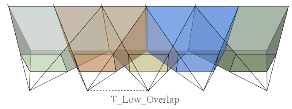
(a) Low overlap spacing

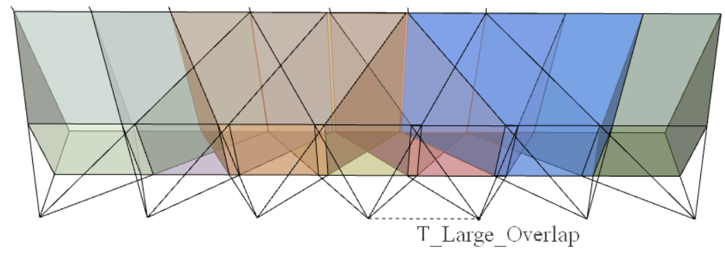
(b) High overlap spacing

Figure 1: The figure illustrates a 3D space occupied by low (a) and high (b) Overlap spacing. Low overlap creates sparse sampling, which leads to a ’hard’ relative-pose-regression problem. High overlap creates dense sampling, which leads to an ’easy’ relative-pose-regression problem. The complexity of a regression problem is affected by the regression subspace volume. In terms of absolute-pose-regression, both are equivalent since we use the same space.

1 Introduction

Visual Simultaneous Localization and Mapping (V-SLAM) is a widely used method in vision-based applications, including mobile robots, virtual reality (VR), augmented reality (AR) and navigation (from domestic environments to rockets and satellites), as well as in many more applications in multifarious fields. Although GPS is a robust and readily available solution for localization, for many applications it is not affordable. Due to its fundamental importance as a core technology for a wide range of applications, visual localization has been extensively studied with major progress evidenced over the past few years [25], [9], [10], [3], [31]. However, accurate and robust localization is still a challenging problem, alongside the growing demands for constructing better maps. If an agent needs to locate itself when a map is given in addition to visual clues, the task is called re-localization [1]. A few examples of re-localization are: loop closure for autonomous navigation, map loading for virtual and augmented reality, and the kidnap robot problem. Re-localization can be viewed as regressing the pose of the camera when prior knowledge is given as a map. In recent years, researchers have used the deep learning approach, and trained a deep neural network to regress the camera pose on a query (test) image, given a set of training images. One of the most effective known techniques is called relative-pose-regression with image retrieval; it is computationally efficient and able to generalize to new unseen scenes, as we will demonstrate herein. Other published works [20], [2], [29], [8] present different implementations and techniques to improve re-localization performance. Detailed evaluations of these and other works were done independently by [39], [32], [34]. However, to the best of our knowledge, our work is the first to take into account the elusive tradeoff that has been overlooked in the comparison criteria published to date. It transpires that choosing different parameters on the same model affects the accuracy of the model, when using the current metrics. In this work, we will demonstrate this tradeoff, both qualitatively and empirically. This paper introduces new metrics that take into account the subspace size. To evaluate our new metrics we used a relative-pose-regression framework for camera re-localization as a baseline for future works. Our Siamese network consists of two equivalent backbones with shared weights. Each learns to encode geometric information from an image into a feature vector. In the test stage, only one of these networks is used to estimate the camera pose. This method is able to generalize well, as we will show 5; we train it on one scene and show that the learned model is able to work well on the other scenes without retraining. We also present a new technique for estimating the amount of correlated information, given a pair of images, based on their location and some prior knowledge on the environment.

To summarize, we offer the following contributions:

• We raise a concern regarding erroneous conclusions drawn in published relative-pose-regression camera methods. We will show that due to neglect of the tradeoff we revealed, some approaches perform favorably in terms of current evaluation metrics, while, in reality, they perform badly.

• We propose to revise the metrics used for evaluating relative-pose-regression camera methods. We propose three metrics, which incorporate some statistics regarding the scene volume. Our new metrics depend on the 3D volume occupied and on how closely viewpoints are sampled.

• We introduce a new way to estimate the amount of correlated information between pairs of images by 3D frustum-overlap. This approach makes the perception of the neglected tradeoff more intuitive.

• We present a better way to use the overlap score, and we demonstrate the robustness and benefits of the relative-pose-regression method that produces competitive results on untrained environments.

The rest of the paper is organized as follows: Sec. 2 briefly reviews the related work in visual re-localization. The details of our approach, network structure, and overlap score function are detailed in Sec. 3. Sec. 4 is devoted to reviewing the comparison criteria. Evaluation results are provided in Sec. 5. In Sec. 6, we summarize the results and conclusions, and offer some suggestions for future work. Our source code will be publicly available soon.

2 Related Work

2.1 Re-localization approaches

The task of camera re-localization has a long history of research in various V-SLAM systems. Traditional approaches, as well as some leading algorithms [30], [3], [12], are built on multi-view geometry theory. Other methods, like appearance-based similarity, the Hough Transform [38], and random-forest based methods [23], [35], [14], have been investigated and shown good results on some benchmarks. Recently, deep learning approaches have become a popular end-to-end solution for re-localization problems [35], [13], [28], [18], instead of only being a replacement for parts of the re-localization pipeline [5]. The benefits of this approach are reduction of the inference time and of memory consumption, which is crucial for low computation and memory devices like drones, AR/VR and mobile devices. The major methods are now briefly summarized.

2.1.1 Features-Based

Methods are methods that use multi-view geometry features extractors and descriptors. This approach is the base for several leading solutions [3], [4], [19], [30], [33]. However, this family of methods has a major drawback: they are limited to a small working area since the computational costs grow significantly with working area size, even after optimization, such as is found in the case presented in [10] and others.

2.1.2 Fiducial Markers

One of the most popular approaches is based on the use of binary square fiducial markers. The main benefit of these markers is that a single marker provides enough correspondences to obtain the camera pose. Every marker is associated with a coordinate system, and poses are given relative to that coordinate system’s origin [40], [27], [11].

2.1.3 Absolute Pose-Regression

The method outlined in [17] suggested learning the re-localization pipeline in an end-to-end supervised manner. The idea of regressing the absolute pose by using machine learning offered several appealing advantages compared to traditional feature-based methods. Deep learning based on absolute pose-regression does not require the design of hand-crafted features. The trained model has a low memory footprint and constant runtime. However, any solution for absolute pose-regression suffers from over-fitting on the training data and will not generalize well - which is a desired property in practical cases. Recently, many learning-based algorithms have been developed [7], [36], [21], [24].

2.1.4 Relative-Pose-Regression with Image Retrieval

The key idea of relative-pose-regression is that once an anchor image has been determined, one can directly regress the relative camera pose between the anchor and test images, and thus obtain the absolute pose. The relative-pose-regression approach requires a definition of similarity. This definition has been proposed and studied recently in several works. The method enjoys many of the advantages of the previously described methods, attractive computational costs stemming from its maintaining a relatively small database, decoupling of the pose-regression process from the coordinate frame of the scene. In addition, it does not require scene-specific training, as we will demonstrate. [20], [23], [31], [37], [8], [22], [29].

2.1.5 Combination of Methods

The authors in [39] presented a multi-task training approach, leveraging relative-pose information during the training, and demonstrated impressive results. Alternatively, a variety of combinations are outlined in [6], where, for sequence localization they combine absolute pose-regression from the current frame to relative pose from the previous frame. In addition, a combination of the new approaches with traditional algorithms has improved the results, such as where the combination was done using visual odometry algorithms, which take as input IMU and GPS sensors. In the test stage, predictions were further refined with pose graph optimization.

2.2 Images Intersection Score

In relative-pose-regression a metric is used to estimate the correlated information between pairs of images, i.e. to determine whether a given pair of images contains enough overlapped information such that the algorithm can retrieve the relative pose between them. A few metrics have evolved during the last few years: the authors in [20] measured the overlap as the percentage of pixels projected onto a candidate image plane using the respective ground truth pose and depth maps; the method in [2] projects depth from one pose, and un-projects it from another, and then counts how many points are on the image plane; the authors in [8] suggested using ORB similarity for outdoor scenes with 2D image data-sets. Both overlap calculation methods use the geometric as well as the visual content of the images. In this work, we propose using pose information from the ground-truth, and do not assume depth information is available. Although each method has its advantages, we think that none provides adequate intuitive understanding of the sub-space that is spread by the span of all the relative pose. To this end we now introduce a new, and more intuitive, image intersection score we call frustum-overlap.

3 Methodology

The main novelty of this work is to revise the problem of re-localization assessment expressed with standard comparison criteria, and to propose a new comparison protocol. We therefore used the popular models and methods that are known to work on the problem, such as camera re-localization.

3.1 Frustum-Overlap - An Intuitive Images Intersection Score

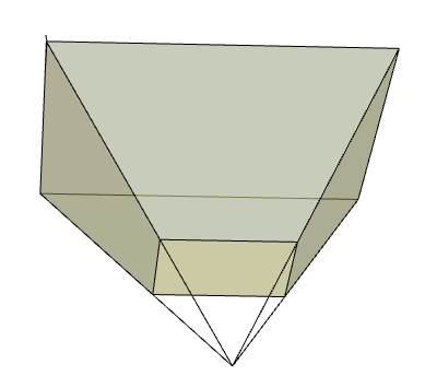
(a) Frustum Type a

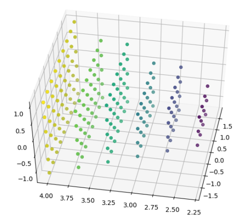
(b) Frustum Type b

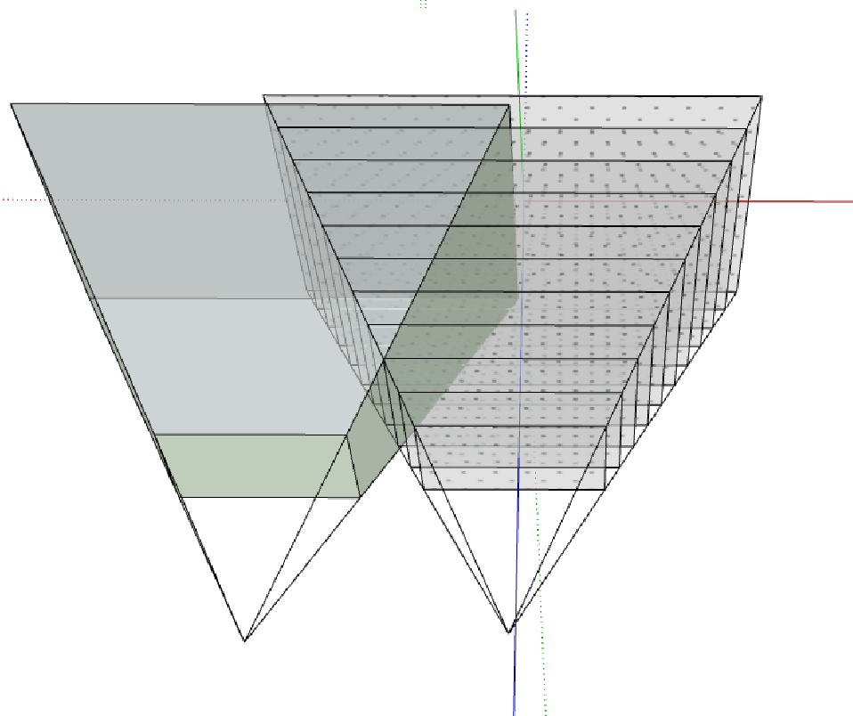
(c)

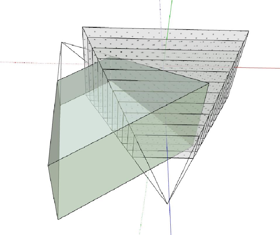
(d)

Figure 2: Frustum types

We introduce a novel definition for image overlap that does not rely on the content of the images. We borrowed the concept of the camera view frustum from computer graphics. A frustum is a truncated pyramid that starts at the focal plane of the camera, and extends up to the maximum viewable distance. We use two different ways to define a frustum:

• Type a is presented in Fig. 2(a) - A set of 6 3D planes, 2 parallel planes and 4 planes delimiting them to a pyramid.

• Type b is presented in Fig. 2(b) - A discrete set of 3D points on a grid, constructing a frustum shape.

To get an overlap score given a pair of two poses, we need to place a frustum of Type a in the first pose and a frustum of Type b in the other pose, and then extract the percentage of 3D points of the second frustum that are inside the first frustum. This is illustrated in Fig. 2(c). In Equation  1 we describe the counting formula we used, to give some informal intuition behind the calculation.

$$\begin{split}&overlap\_score=\sum_{p_{i}\in frustum\_a}\frac{a_{i}}{N_{b}}\\ &a_{i}=\begin{cases}1,&\text{if $p_{i}$ is in frustum\_b}\\ 0,&\text{otherwise}\\ \end{cases}\\ \end{split}$$ (1)

Our overlap scoring method. $N_{b}$ is the total number of points in frustum b.

This approach has a major drawback - it is possible to get a high overlap score for two images without any common visual content (see Fig. 2(d) for an illustration.) We overcome this drawback by limiting the relative rotation between two captures. It is important to emphasize that, in contrast to other methods, our method scores overlap in 3D space, and therefore has a tight relationship with the span subspace. A formal definition of the calculation of the score is given in the supplementary material.

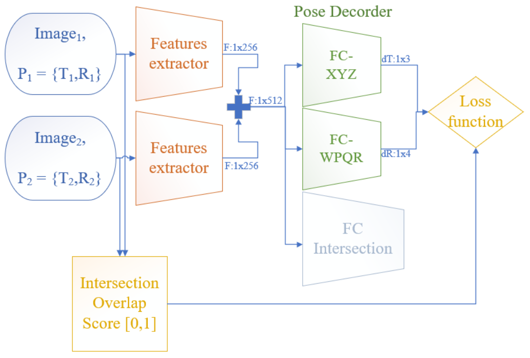
Figure 3: Diagram of the proposed training architecture: each Siamese branch uses a shared features extractor to get a representation of the image. The pose decoder predicts rotation, represented by a quaternion, and translation, using ${x,y,z}$ coordinates.

3.2 Training Procedure

Our training procedure is done in a straightforward way. Given the pre-defined pairs of images induced by the selection of the overlap computing method and overlap threshold, as well as their corresponding relative pose as a label, we leverage Siamese architecture to get the estimated relative pose for the network. A schematic of our training procedure is given in Figure 3.

3.3 Loss Function

Loss definition for supervised pose-regression tasks is challenging because it involves learning two distinct quantities - rotation and translation. Each has its own different units and different scales. The authors in [16] found that outdoor and indoor scenes are characterized by different weights, which motivates to dynamically learn the weights of the loss for each task instead of determining them in a hard-coded manner. We follow this notion and use learned $\alpha$ and $\beta$ to balance the losses and combine them, as described formally in [16]:

$$L_{q}(\hat{q_{rel}},q_{rel})=\left\lVert q_{rel}-\frac{\hat{q_{rel}}}{\left\lVert{\hat{q_{rel}}}\right\rVert_{2}}\right\rVert_{2}$$ (2a)

$$L_{t}(\hat{t_{rel}},t_{rel})=\left\lVert t_{rel}-{\hat{t_{rel}}}\right\rVert_{2}$$ (2b)

$$L(\hat{p_{rel}},p_{rel})=\alpha^{2}+\beta^{2}+e^{-\alpha^{2}}L_{t}(\hat{t_{rel}},t_{rel})+e^{-\beta^{2}}L_{q}(\hat{q_{rel}},q_{rel})$$ (2c)

where $t_{rel}$ and $q_{rel}$ are the relative translation and rotation of the $\hat{}$ superscript that denotes predicted values. This form of loss function makes it possible for us to learn the weighting between the translation and rotation objectives and to find optimal weighting for a specific data-set.

4 Comparison Criteria

4.1 Standard Comparison Criteria

To evaluate the performance of the proposed algorithm, we require a set of images and their corresponding ground truth poses. We estimate the image poses predicted by the algorithm and calculate the pose error for translation and rotation. The popular localization metrics are:

$$t_{err}(\hat{t}_{i},t_{i})=\|{t_{i}-\hat{t_{i}}}\|_{2}$$ (3a)

$$q_{err}(\hat{q}_{i},q_{i})=\frac{180}{\pi}2\cos^{-1}(<q_{i},\hat{q_{i}}>)$$ (3b)

After obtaining a set of translation and rotation errors, a statistical measure to convert them to a single scalar score is used. Common choices [6], [17], [2] are the mean and the median:

$$T_{err}=mean/median(\{t_{err}(\hat{t}_{i},t_{i})\}_{i\in N})$$ (4a)

$$Q_{err}=mean/median(\{q_{err}(\hat{q}_{i},q_{i})\}_{i\in N})$$ (4b)

4.2 The limitations of standard comparison criteria

In absolute-pose-regression, when one calculates the error using Equation 4 the scale (regression subspace volume) is implicitly involved in the computation. The error is limited by the scene dimensions, and can be manipulated by normalizing the scene. Moreover, the train and test sets are exactly the same, because there is no pre-defined overlap based selection. In relative-pose-regression, this is not the case; the selection of the overlap method and threshold implicitly determines the complexity of the problem, errors are limited by this selection and scene normalization will not solve it. Changing either the overlap calculation method or the threshold might significantly change the train and test data. An illustration of this key insight is depicted in Figure 1. Qualitatively, if one chooses ’high’ overlap, the regression subspace volume is smaller than if one choses ’low’ overlap. This, in turn, will lead at first sight to the conclusion that the algorithm that trained and tested on ’high’ overlap is better, but we argue that this is not necessarily so. We further argue that there is a strong correlation between the spanned 3D volume induced by the overlap selection and the performance of the selected algorithm, as we will show in section 5. We demonstrate this claim visually in Figure 4

(a)

model a
15 epochs of training
100 pairs of images
Minimum overlap of 0.4
Subspace size: $1\times 0.5\times 0.8=0.4[m^{3}$]
Mean translation : 0.11 [m]
Mean Rotation: 3.51 [degree]

(b)

model b
1 epoch of training
100 pairs of images
Minimum overlap of 0.95
Subspace sizes: $0.6\times 0.25\times 0.3=0.045[m^{3}$]
Mean translation : 0.10 [m]
Mean Rotation: 3.39 [degree]

Figure 4: The figures present the translations error of two models. Red and green points are ground truths and estimates, respectively. Considering only the numerical results the naive model (b) is better. However, after visual examination, it is clear that model (b) is worthless, while model (a) learned to predict the pose. The mistake stems from not taking the subspace volume into account.

	RelocNet [2]	NNnet[20]	Anchornet [29]	CamNet[8]	Ours
Scene	RPR	RPR	RPR	RPR	RPR
Chess	0.12m, 4.14∘	0.13m, 6.46∘	0.08m, 4.12∘	0.04m, 1.73∘	0.03m, 1.36∘
Fire	0.26m, 10.4∘	0.26m, 12.72∘	0.16m, 11.1∘	0.03m, 1.74∘	0.03m, 1.92∘
Heads	0.14m, 10.5∘	0.14m, 12.34∘	0.09m, 11.2∘	0.05m, 1.98∘	0.03m, 3.18∘
Office	0.18m, 5.32∘	0.21m, 7.35∘	0.11m, 5.38∘	0.04m, 1.62∘	0.03m, 1.75∘
Pumpkin	0.26m, 4.17∘	0.24m, 6.35∘	0.14m, 3.55∘	0.04m, 1.64∘	0.03m, 0.98∘
Kitchen	0.23m, 5.08∘	0.24m, 8.03∘	0.13m, 5.29∘	0.04m, 1.63∘	0.03m, 1.11∘
Stairs	0.28m, 7.53∘	0.27m, 11.80∘	0.21m, 11.9∘	0.04m, 1.51∘	0.03m, 1.27∘

Table 1: The table demonstrates the inadequacy of the existing criterion. We adjusted the overlap parameter to get results that seem better than those of the other methods. However, we emphasize that this is not sufficient to determine which method is preferable.

	Active search	DSAC++	Posenet	Posenet Geometric	MapNet	CamNet	Ours
	3D	3D	APR	APR	APR	RPR	RPR
Chess	0.04m,1.96∘	0.02m, 0.5∘	0.32m, 6.60∘	0.13m, 4.48∘	0.08m, 3.25∘	0.04m, 1.73∘	0.03m, 1.36∘
Fire	0.03m,1.53∘	0.02m, 0.9∘	0.47m, 14.0∘	0.27m, 11.3∘	0.27m, 11.69∘	0.03m, 1.74∘	0.03m, 1.92∘
Heads	0.02m,1.45∘	0.01m, 0.8∘	0.30m, 12.2∘	0.17m, 13.0∘	0.18m, 13.25∘	0.05m, 1.98∘	0.03m, 3.18∘
Office	0.09m,3.61∘	0.03m, 0.7∘	0.48m, 7.24∘	0.19m, 5.55∘	0.17m, 5.15∘	0.04m, 1.62∘	0.03m, 1.75∘
Pumpkin	0.08m,3.10∘	0.04m, 1.1∘	0.49m, 8.12∘	0.26m, 4.75∘	0.22m, 4.02∘	0.04m, 1.64∘	0.03m, 0.98∘
Kitchen	0.07m,3.37∘	0.04m, 1.1∘	0.58m, 8.34∘	0.23m, 5.35∘	0.23m, 4.93∘	0.04m, 1.63∘	0.03m, 1.11∘
Stairs	0.03m,2.22∘	0.09m, 2.6∘	0.48m, 13.1∘	0.35m, 12.4∘	0.30m, 12.08∘	0.04m, 1.51∘	0.03m, 1.27∘

Table 2: Misleading comparison to other methods (APR: absolute-pose-regression, RPR: relative-pose-regression, 3D-classical) using the standard median metric on 7-scenes data-set.

4.3 Proposed Metrics

As a direct sequitur to the previous sections, the results obtained using a naive implementation of Equation 4 is not enough to make a fair comparisons. As mentioned earlier, we claim that in regression methods comparison with Equation 4 is reliable only if their volume is similar. However, in the case where we do not know the subspace volume we need other information in order to get a reliable comparison. Hence, our first suggestion is to use a sub-space agnostic metric. As a minimal requirement for fair comparison, one should include the subspace volume or a statistical representation of it.

4.3.1 Statistical Criteria Inspired from Financial Analysis

• The mean absolute percentage error (MAPE), defined as:

  $$T_{MAPE}=\frac{1}{N}\sum_{i\in N}(\frac{|t_{i}-\hat{t_{i}}|_{1}}{|t_{i}|_{1}})$$ (5)

  The intuition behind this metric is: penalty decreases proportionally with the distance from the origin. Hence, it implies a larger penalty on errors in ’smaller’ scenes [26].
  

• The mean absolute scaled error (MASE) is another relative measure of the error. It is defined as the mean absolute error of the model divided by the mean absolute error of a naive random-walk-without-drift model (the mean absolute value of the first difference of the series) [15]. Thus, it measures the relative error compared to a naive model:

  $$T_{MASE\_error}=\frac{T_{MAE}}{T_{Naive}}=\frac{\sum_{i\in N}(|t_{i}-\hat{t_{i}}|)}{\sum_{i\in N}{|t_{i}-mean(\{|t|\}_{i\in N}|}}$$ (6)

• The mean absolute percentage scaled error (MAPSE) is a combination of the two measures mentioned above. The benefits of using this measure are better normalization and scale-less errors:

  $$T_{MAPSE\_error}=\frac{T_{MAPE}}{T_{Naive}}=\frac{\sum_{i\in N}(\frac{|t_{i}-\hat{t_{i}}|}{|t_{i}|})}{\sum_{i\in N}{|t_{i}-mean(\{|t|\}_{i\in N}|}}$$ (7)

We visually illustrate these measures in Figure 5

The claims are valid for both rotation and translation. Subspace volume is not intuitive in quaternions representation, but if we convert to Euler angles we can use the same formulas. The subspace of absolute orientation in most scenes is the full sphere, but for the rotation (relative orientation) it is also much smaller. The ”MAPE” formula is given by:

$$R_{MAPE}(EulerAngles)=\frac{1}{N}\sum_{i\in N}(\frac{|r_{i}-\hat{r_{i}}|}{|r_{i}|})$$ (8)

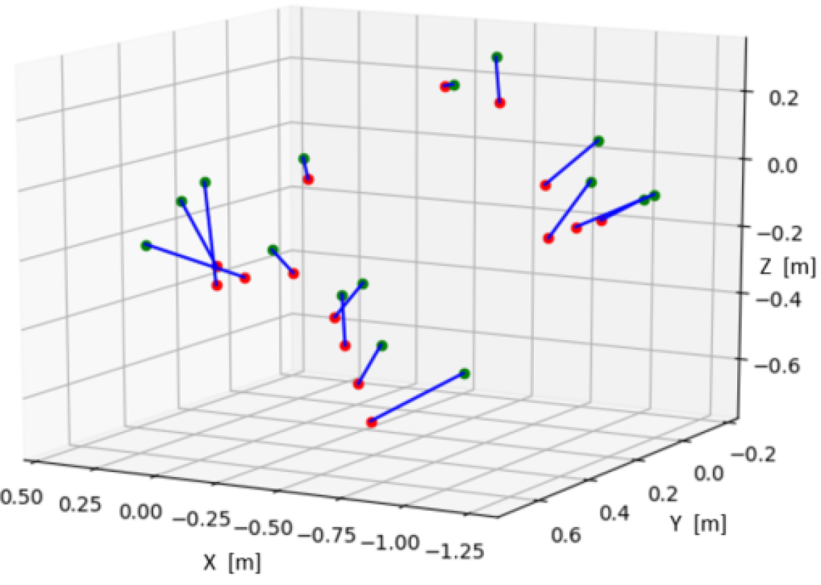
(a) Translation error vector

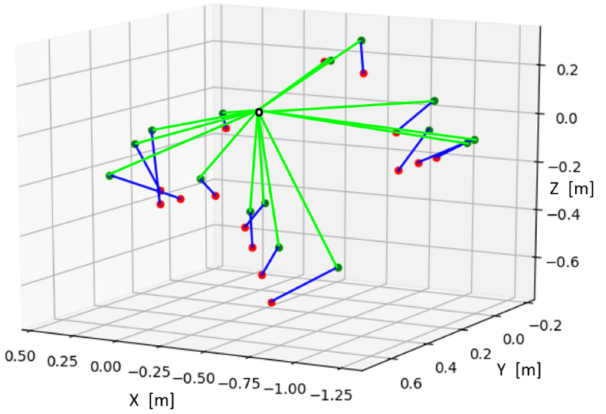
(b) Mean Absolute Percentage Error (MAPE)

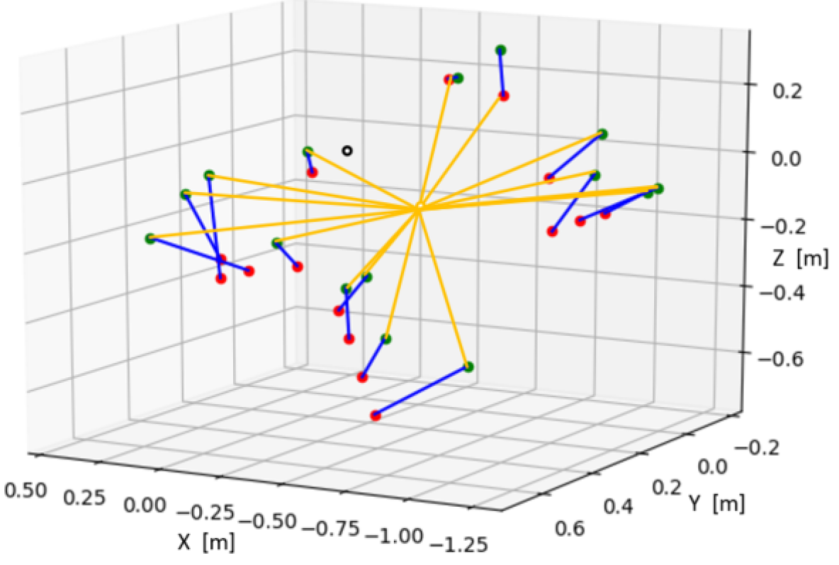
(c) Mean Absolute Scale Error (MASE)

Figure 5: An Illustration of the proposed metrics. Ground truth points are in green, estimation points in red, the blue line connected them is the translation error. Green and yellow lines represent the normalization factor of the error in MAPE and MASE, respectively. These types of normalization are necessary when subspace volume is taken into account.

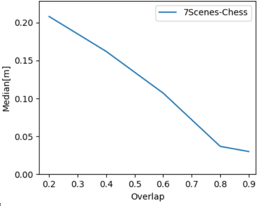
(a)

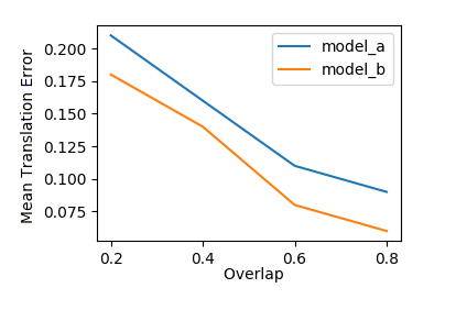
(b)

Figure 6: (a) Accuracy across different overlaps on 7-scenes data-set. We can see clearly the correlation, when overlap increase accuracy decrease. (b) Two trained models tested on the same data. We can see that Model b performs better than Model a since it valid for any overlap score. To evaluate and compare in cases there is no single model that is always better, we turned to the area under the curve (AUC) approach.

4.3.2 Area under curve for all overlap ranges

The accuracy of a model depends on how well it estimates the relative pose given a test pair of images. As mentioned earlier, the selection of the overlap method and threshold significantly determines the complexity of the problem. In order to achieve a non-overlap dependence on assessment, one way is to compute the area under the curve (AUC) across the overlaps. The model is better as the area decreases. Quantification of the difference between the two models could be obtained from the difference between their AUCs. This is illustrated in Fig LABEL:fig:AUC.

4.3.3 Minimal requirement for reliable comparison

As a relaxation of the previous method, it might be enough to consider the sub-space diameter. Intuitively, the subspace diameter quantifies the spanned 3D space induced by the relative pose targets (labels). The sub-space diameter can be defined as:

$$subspace\_diameter=mean(\{|t|\}_{i\in N})+2{std(\{|t|\}_{i\in N})}$$ (9)

	Overlap Threshold
	0.2	0.4	0.6	0.8	0.9
Chess	1.95	1.91	1.54	0.71	0.57
Fire	1.65	1.16	0.80	0.77	0.68
Heads	2.13	1.93	1.13	0.57	0.45
Office	2.79	2.65	2.28	0.92	0.42
Pumpkin	1.24	1.34	1.42	0.80	0.26
Kitchen	3.49	2.47	1.76	0.88	0.38
Stairs	0.91	0.75	0.60	0.50	0.37

(a) Demonstrated on 7-scenes[35] data-set.

	Overlap Threshold
	0.2	0.4	0.6	0.8	0.9
Kings Collage	6.82	4.87	3.51	2.50	1.26
Great Court	6.54	5.00	3.59	2.39	1.58
Old Hospital	8.08	6.71	5.16	2.73	0.89
St M. Church	8.43	7.21	5.61	2.40	0.69
Streets	6.48	4.78	3.56	2.45	1.14
Shop Facade	6.08	4.28	3.79	2.42	1.43

(b) Demonstrated on Cambridge[17] data-set.

Table 3: Relative poses regression subspace diameter in meters as a function of overlap. The subspace created by the span of all relative-poses with enough overlap. The diameters are correlated to overlap threshold, while the scene volume almost not matter.

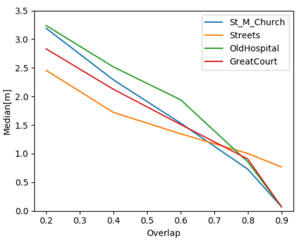
(a) Median accuracy across different overlaps on Cambridge data-set.

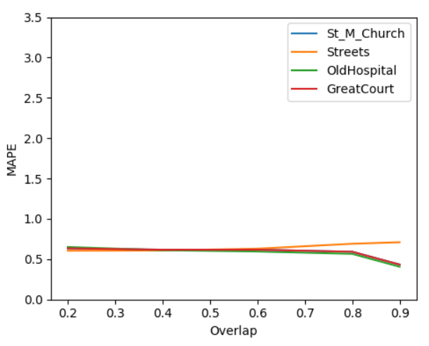
(b) MAPE across different overlaps on Cambridge data-set.

Figure 7: Translation error using median (a) and using MAPE (b) across different overlaps.

5 Experiments and Results

5.0.1 Comparison to other methods

: To demonstrate our key insights we conducted several experiments. We chose the 7-Scenes data-set [35] and trained our architecture (see section 3). As its name implies, this data-set consists of 7 different scenes taken using a Microsoft Kinnect camera. For each of these scenes, we compare our trained network using an appropriate overlap threshold to achieve satisfactory results. These experiments are summarized in Table 2. It is worth noting that our comparison is not complete. The train and test data are not the same, due to pairs selection induced by the overlap method. At first sight, our method yields the best results compared to other methods. However, one should note that we chose the overlap accordingly in order to achieve better results using the common criteria metrics. This complies with what was argued in 4.2.

5.0.2 Comparison to relative-pose methods

: We compare our method using the standard median to other relative-pose methods. Note that these comparisons are made without relating to the sub-space diameter, and are summarized in Table 1.

5.0.3 Correlation between sub-space diameter and accuracy

: To analyze the correlation with sub-space diameter as defined in Section 4, we measure the sub-space diameter for each scene over a range of different overlaps. We introduce here another data-set we used, called Cambridge [17]. Results are summarized in Table LABEL:table:overlap_diameter. To prove empirically our claim that there is a strong correlation between overlap and accuracy, we trained the Chess scene from the 7-scenes data-set with an overlap of 0.6 and tested it under various overlap ranges. Results are shown in Figure 6(a).

5.0.4 Volume agnostic methods

: We offer sub-space diameter agnostic metrics. By agnostic, we mean that the proposed measure should be stable under different overlap and threshold selection methods. We used our trained model on the Chess scene from the 7-scenes data-set. We evaluated the methods proposed in section 4.3 and showed that the metrics result is stable around the same values, even when we modified the overlap threshold. These results are summarized in Figure 8. We also changed the common definition of MAPE and MASE, and used $L2$ as a norm to examine the robustness of our method to norm selection. Results are summarized in Figure 9.

Figure 8: An illustration of using volume-agnostic metrics vs median metric under L1 norm. The blue line at each plot is the median, when the other line in each plot is one of the 3 proposed metrics. It can be clearly seen that the proposed method is robust to different overlaps.

Figure 9: Proposed metrics are agnostic to norm selection. Unlike Fig. 8 here we use $L2$. It can be seen that the proposed metrics are robust to norm selection.

	AnchorNet		Ours best		Ours chess model
	Accuracy	Subspace Diameter	Accuracy	Subspace Diameter	Accuracy	Subspace Diameter
chess	0.08m, 4.12∘	0.19	0.07m, 1.63∘	0.19	0.07m, 1.63∘	0.19
fire	0.16m, 11.1∘	0.14	0.02m, 1.45∘	0.14	0.16m, 6.25∘	0.14
Heads	0.09m, 11.2∘	0.05	0.02m, 1.73∘	0.05	0.07m, 3.43∘	0.05
Office	0.11m, 5.38∘	0.18	0.02m, 1.53∘	0.18	0.12m, 4.35∘	0.18
Pumpkin	0.14m, 3.55∘	0.11	0.02m, 1.09∘	0.11	0.09m, 3.96∘	0.11
Red Kitchen	0.13m, 5.29∘	0.22	0.02m, 1.14∘	0.22	0.10m, 4.06∘	0.22
Stairs	0.21m, 11.9∘	0.17	0.01m, 0.74∘	0.17	0.10m, 2.54∘	0.17

Table 4: Comparison to [29] given the subspace diameter. Note that in the third double-column we train only on one scene and yet are able to generalize to other scenes as well.

5.0.5 Comparison given sub-space diameter

: As we mentioned earlier, a minimal requirement for fair comparison is referred to as the subspace diameter, as reported in [29]. Hence, we compare our method to theirs, as summarized in Table LABEL:tab:compare_sub_space_diameter.

6 Conclusions

In this paper, we introduce a novel comparison criterion for relative-pose-regression. We demonstrate the insufficiency of the current standard metrics in terms of their capability to assess relative-pose-regression algorithms. We also show that our proposed metrics overcome many of the drawbacks of existing metrics, and believe that the proposed metrics should be adopted in the field. We believe that relative-pose-regression is crucial for solving the problem of camera re-localization. Generalization (training on one scene and achieving good results on another) is a key to the widely-adopted full solution of the problem; however, we leave its extensive investigation for future work.

In our opinion, due to the lack of generalization capabilities of the absolute pose-regression approach, relative-pose-regression is now the most promising research direction in data-driven visual re-localization.

References

- [1] Argamon, S., McDermott, D.: Error correction in mobile robot map learning. Proceedings 1992 IEEE International Conference on Robotics and Automation pp. 2555–2560 vol.3 (1992)
- [2] Balntas, V., Li, S., Prisacariu, V.: Relocnet: Continuous metric learning relocalisation using neural nets. In: The European Conference on Computer Vision (ECCV) (September 2018)
- [3] Brachmann, E., Krull, A., Nowozin, S., Shotton, J., Michel, F., Gumhold, S., Rother, C.: Dsac — differentiable ransac for camera localization. 2017 IEEE Conference on Computer Vision and Pattern Recognition (CVPR) pp. 2492–2500 (2016)
- [4] Brachmann, E., Rother, C.: Learning less is more - 6d camera localization via 3d surface regression. 2018 IEEE/CVF Conference on Computer Vision and Pattern Recognition pp. 4654–4662 (2017)
- [5] Brachmann, E., Rother, C.: Expert sample consensus applied to camera re-localization. 2019 IEEE/CVF International Conference on Computer Vision (ICCV) pp. 7524–7533 (2019)
- [6] Brahmbhatt, S., Gu, J., Kim, K., Hays, J., Kautz, J.: Geometry-aware learning of maps for camera localization. 2018 IEEE/CVF Conference on Computer Vision and Pattern Recognition pp. 2616–2625 (2017)
- [7] Cavallari, T., Golodetz, S., Lord, N.A., Valentin, J.P.C., di Stefano, L., Torr, P.H.S.: On-the-fly adaptation of regression forests for online camera relocalisation. 2017 IEEE Conference on Computer Vision and Pattern Recognition (CVPR) pp. 218–227 (2017)
- [8] Ding, M., Wang, Z., Sun, J., Shi, J., Luo, P.: Camnet: Coarse-to-fine retrieval for camera re-localization. In: The IEEE International Conference on Computer Vision (ICCV) (October 2019)
- [9] Engel, J., Koltun, V., Cremers, D.: Direct sparse odometry. IEEE Transactions on Pattern Analysis and Machine Intelligence 40, 611–625 (2016)
- [10] Engel, J., Schöps, T., Cremers, D.: Lsd-slam: Large-scale direct monocular slam. In: ECCV (2014)
- [11] Fiala, M.: Artag, a fiducial marker system using digital techniques. 2005 IEEE Computer Society Conference on Computer Vision and Pattern Recognition (CVPR’05) 2, 590–596 vol. 2 (2005)
- [12] Gálvez-López, D., Tardós, J.D.: Bags of binary words for fast place recognition in image sequences. IEEE Transactions on Robotics 28(5), 1188–1197 (October 2012). https://doi.org/10.1109/TRO.2012.2197158
- [13] Gordo, A., Almazán, J., Revaud, J., Larlus, D.: Deep image retrieval: Learning global representations for image search. In: European conference on computer vision. pp. 241–257. Springer (2016)
- [14] Guzmán-Rivera, A., Kohli, P., Glocker, B., Shotton, J., Sharp, T., Fitzgibbon, A.W., Izadi, S.: Multi-output learning for camera relocalization. 2014 IEEE Conference on Computer Vision and Pattern Recognition pp. 1114–1121 (2014)
- [15] Hyndman, R.J., Koehler, A.B.: Another look at measures of forecast accuracy. In: FORESIGHT (2006)
- [16] Kendall, A., Cipolla, R.: Geometric loss functions for camera pose regression with deep learning. 2017 IEEE Conference on Computer Vision and Pattern Recognition (CVPR) pp. 6555–6564 (2017)
- [17] Kendall, A., Grimes, M.K., Cipolla, R.: Posenet: A convolutional network for real-time 6-dof camera relocalization. 2015 IEEE International Conference on Computer Vision (ICCV) pp. 2938–2946 (2015)
- [18] Larsson, M., Stenborg, E., Toft, C., Hammarstrand, L., Sattler, T., Kahl, F.: Fine-grained segmentation networks: Self-supervised segmentation for improved long-term visual localization. In: The IEEE International Conference on Computer Vision (ICCV) (October 2019)
- [19] Laskar, Z., Huttunen, S., DanielHerrera, C., Rahtu, E., Kannala, J.: Robust loop closures for scene reconstruction by combining odometry and visual correspondences. 2016 IEEE International Conference on Image Processing (ICIP) pp. 2603–2607 (2016)
- [20] Laskar, Z., Melekhov, I., Kalia, S., Kannala, J.: Camera relocalization by computing pairwise relative poses using convolutional neural network. 2017 IEEE International Conference on Computer Vision Workshops (ICCVW) pp. 920–929 (2017)
- [21] Massiceti, D., Krull, A., Brachmann, E., Rother, C., Torr, P.H.S.: Random forests versus neural networks — what’s best for camera localization? 2017 IEEE International Conference on Robotics and Automation (ICRA) pp. 5118–5125 (2016)
- [22] Melekhov, I., Ylioinas, J., Kannala, J., Rahtu, E.: Relative camera pose estimation using convolutional neural networks. In: ACIVS (2017)
- [23] Meng, L., Chen, J., Tung, F., Little, J.J., Valentin, J., de Silva, C.W.: Backtracking regression forests for accurate camera relocalization. 2017 IEEE/RSJ International Conference on Intelligent Robots and Systems (IROS) pp. 6886–6893 (2017)
- [24] Meng, L., Tung, F., Little, J.J., Valentin, J., de Silva, C.W.: Exploiting points and lines in regression forests for rgb-d camera relocalization. 2018 IEEE/RSJ International Conference on Intelligent Robots and Systems (IROS) pp. 6827–6834 (2017)
- [25] Mur-Artal, Montiel, R., Juan, T.: Orb-slam: a versatile and accurate monocular slam system. IEEE Transactions on Robotics 31(5), 1147–1163 (2015)
- [26] Myttenaere, A.D., Golden, B., Grand, B.L., Rossi, F.: Mean absolute percentage error for regression models. Neurocomputing 192, 38–48 (2016)
- [27] Pfrommer, B., Daniilidis, K.: Tagslam: Robust slam with fiducial markers. ArXiv abs/1910.00679 (2019)
- [28] Radenović, F., Tolias, G., Chum, O.: Cnn image retrieval learns from bow: Unsupervised fine-tuning with hard examples. In: ECCV (2016)
- [29] Saha, S., Varma, G., Jawahar, C.V.: Improved visual relocalization by discovering anchor points. In: BMVC (2018)
- [30] Sattler, T., Leibe, B., Kobbelt, L.: Improving image-based localization by active correspondence search. In: ECCV (2012)
- [31] Sattler, T., Leibe, B., Kobbelt, L.: Efficient & effective prioritized matching for large-scale image-based localization. IEEE Transactions on Pattern Analysis and Machine Intelligence 39, 1744–1756 (2017)
- [32] Sattler, T., Zhou, Q., Pollefeys, M., Leal-Taixé, L.: Understanding the limitations of cnn-based absolute camera pose regression. ArXiv abs/1903.07504 (2019)
- [33] Schönberger, J.L., Pollefeys, M., Geiger, A., Sattler, T.: Semantic visual localization. 2018 IEEE/CVF Conference on Computer Vision and Pattern Recognition pp. 6896–6906 (2017)
- [34] Shavit, Y., Ferens, R.: Introduction to camera pose estimation with deep learning (2019)
- [35] Shotton, J., Glocker, B., Zach, C., Izadi, S., Criminisi, A., Fitzgibbon, A.W.: Scene coordinate regression forests for camera relocalization in rgb-d images. 2013 IEEE Conference on Computer Vision and Pattern Recognition pp. 2930–2937 (2013)
- [36] Svärm, L., Enqvist, O., Kahl, F., Oskarsson, M.: City-scale localization for cameras with known vertical direction. IEEE Transactions on Pattern Analysis and Machine Intelligence 39, 1455–1461 (2017)
- [37] Taira, H., Okutomi, M., Sattler, T., Cimpoi, M., Pollefeys, M., Sivic, J., Pajdla, T., Torii, A.: Inloc: Indoor visual localization with dense matching and view synthesis. 2018 IEEE/CVF Conference on Computer Vision and Pattern Recognition pp. 7199–7209 (2018)
- [38] Tejani, A., Tang, D., Kouskouridas, R., Kim, T.K.: Latent-class hough forests for 3d object detection and pose estimation. In: ECCV (2014)
- [39] Valada, A., Radwan, N., Burgard, W.: Deep auxiliary learning for visual localization and odometry. In: 2018 IEEE International Conference on Robotics and Automation (ICRA). pp. 6939–6946. IEEE (2018)
- [40] Wang, J., Olson, E.: Apriltag 2: Efficient and robust fiducial detection. 2016 IEEE/RSJ International Conference on Intelligent Robots and Systems (IROS) pp. 4193–4198 (2016)