Equilibrium Field Theory of Magnetic Monopoles in Degenerate Square Spin Ice: Correlations, Entropic Interactions, and Charge Screening Regimes

Abstract

We describe degenerate square spin as an ensemble of magnetic monopoles coupled via an emergent entropic field that subsumes the effect of the underlying spin vacuum. We compute their effective free energy, entropic interaction, correlations, screening, and structure factors that coincide with the experimental ones. Unlike in pyrochlore ices, a dimensional mismatch between real and entropic interactions leads to weak singularities at the pinch points and algebraic correlations at long distance. This algebraic screening can be, however, camouflaged by a pseudo-screening regime.

Introduction. Magnetic monopoles Ryzhkin (2005); Castelnovo et al. (2008) provide an emergent description of the low energy physics of rare earth spin ices Ramirez et al. (1999); den Hertog and Gingras (2000); Bramwell and Gingras (2001) and have raised considerable interest, in particular in regard to “magnetricity”  Morris et al. (2009); Giblin et al. (2011); blundell2012monopoles; Kirschner et al. (2018). Spin ices can be modeled den Hertog and Gingras (2000); Henley (2005); Isakov et al. (2004) as systems of Ising spins on a pyrochlore lattice, impinging on tetrahedra, such that their low energy state obeys the Bernal-Fowler ice rule Giauque and Stout (1936); Bernal and Fowler (1933); Pauling (1935): two spins point in, two out of each tetrahedron, realizing a degenerate manifold of constrained disorder Henley (2010); Castelnovo (2010) and residual entropy Pauling (1935); Ramirez et al. (1999). Then, violations of the ice rule can be interpreted as sinks or sources of the magnetization, i.e. charges, and the low energy physics of spin ice can be described in terms of mobile, deconfined, magnetic monopoles, interacting via a Coulomb law, in a disordered spin vacuum. Spin ice is thus a prominent platform in which monopole physics can be investigated.

While experimental probes of monopoles in crystal-grown spin ices are necessarily indirect and at low temperature, magnetic monopoles can now be characterized directly in real time, real space Ladak et al. (2011); Mengotti et al. (2010); Zhang et al. (2013); Farhan et al. (2019) at desired temperature and fields in artificial spin ices. Tanaka et al. (2006); Wang et al. (2006); Nisoli et al. (2013); Heyderman and Stamps (2013); Ortiz-Ambriz et al. (2019) These 2D arrays of magnetic, frustrated nanoislands are fabricated in a variety of geometries, often for exotic behaviors not found in natural magnets. Morrison et al. (2013); farhan2017nanoscale; Bhat et al. (2014); shi2018frustration; Nisoli (2018); Skjærvø et al. (2019); Gliga et al. (2019); sklenar2019field

Here we study the monopoles of degenerate artificial square ice, Möller and Moessner (2006); Schanilec et al. (2019) recently realized in nanopatterned magnets Perrin et al. (2016); Östman et al. (2018); Farhan et al. (2019) and in a quantum annealer King et al. (2020). Square ice provides a direct 2D analogue of 3D pyrochlore spin ice where monopole excitations can be directly characterized. Heuristic field theories of rare earth pyrochlores Henley (2005); Isakov et al. (2004); Henley (2010); Castelnovo (2010) have dealt only with the ice manifold, via a coarse grained, solenoidal field that describes the spin texture. We propose instead a framework where magnetic monopoles are the constitutive degrees of freedom, while the underlying spin ensemble is subsumed into entropic forces among these topological defects.

We show that, in absence of physical interaction King et al. (2020), monopoles interact entropically via a 2D-Coulomb, logarithmic law, leading to $(2+1)$ electromagnetism, Bessel correlations of finite screening length for $T>0$, and thus a conductive phase berezinskii1971destruction; Kosterlitz and Thouless (1973) where monopoles are unbound. The correlation length diverges exponentially as $T\downarrow 0$, signaling the criticality of the ice manifold. Then, inclusion of the monopole-monopole 3D-Coulomb interaction, leads, unlike in 3D spin ice, to algebraic correlations and weak singularities in the structure factor at $T\neq 0$. Its interplay with the entropic interaction drives screening regimes of effectively bound and unbound monopoles.

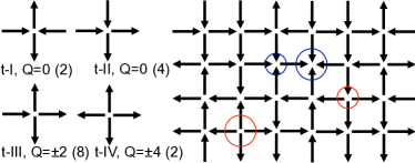
Figure 1: Left: the four vertex configurations, ice-rule ones at the top ($Q=0$) and monopole at the bottom (multiplicities in parenthesis). Right: portion of spin ice with monopoles of different charge circled.

1. Field Theory. Square ice is a set of $N_{e}$ classical, binary spins $\vec{S}_{e}$ aligned on the edges $e$ of a square lattice of unit vectors $\hat{e}_{1},\hat{e}_{2}$, of $N_{v}=N_{e}/2$ vertices labeled by $v$. The 16 spin configurations of a vertex are classified by 4 topologies Wang et al. (2006); Perrin et al. (2016) as t-I, …, t-IV (Fig. 1). Of each vertex, the charge $Q_{v}=2n-4$ is equal to the number $n$ of spins pointing in minus the $4-n$ pointing out. Then, $Q=0$ for ice-rule obeying vertices (t-I, t-II). The following

$${\cal H}[Q]=\frac{\epsilon}{2}\sum_{v}Q_{v}^{2}+\frac{\mu}{2}\sum_{v\neq v^{\prime}}Q_{v}V_{vv^{\prime}}Q_{v^{\prime}},$$ (1)

is a suitable Hamiltonian for a variety of square ice realizations: $\epsilon$ is the cost of monopoles and $V_{vv^{\prime}}=1/2\pi|v-v^{\prime}|$ is their 3D-Coulomb interaction; we take the lattice constant $a=1$ and thus $\mu$ is an energy. When $\mu/\epsilon<2\pi/M_{\square}\simeq 3.9$ (where $M_{\square}\simeq 1.6155$ is our Madelung constant Borwein et al. (1985)) the ground state is a disordered tessellation of the six ice rule vertices (Fig. 1) of known Pauling entropy Lieb (1967); Baxter (1982). Above that threshold, the ground state becomes unstable toward the formation of a monopole ionic crystal.

In magnetic realizations, Perrin et al. (2016); Östman et al. (2018); Farhan et al. (2019) Eq. (1) corresponds to the dumbbell model of ref Castelnovo et al. (2008) (then $\epsilon$ is the coupling of the dumbbell charges in the vertex) with the 3D-Coulomb interaction comes from the usual truncated multipole expansion, and therefore $\mu={\mu_{0}p^{2}}/{l_{d}^{2}}$, with $p$ the magnetic moment, $l_{d}<a$ the dumbbell length. Then, $\mu/\epsilon\simeq 1-l_{d}/a<1$. Equation (1) does not describe the standard, non-degenerate square ice Wang et al. (2006); Nisoli et al. (2010); Morgan et al. (2010); Zhang et al. (2013); Porro et al. (2013); Sendetskyi et al. (2019) in which monopoles are confined by the tension of magnetic Faraday lines.Mól et al. (2009); silva2012thermodynamics; silva2013nambu; Levis et al. (2013); Nisoli (2020); foini2013static Finally, even in realizations where ice-rule vertices are degenerate Möller and Moessner (2006); Perrin et al. (2016); Östman et al. (2018); Schanilec et al. (2019); King et al. (2020), the long ranged dipolar interaction favors antiferromagnetic ordering Perrin et al. (2016) at $T\ll\epsilon$, an effect that we consider here elsewhere.

The partition function is

$$Z\left[H\right]=\sum_{S}\exp{\!\left(-\beta{\cal H}+\beta\sum_{e}\vec{S}_{e}\cdot\vec{H}_{e}\right)},$$ (2)

($\beta=1/T$) such that $\langle\vec{S}_{e_{1}}\dots\vec{S}_{e_{n}}\rangle=\partial_{\beta\vec{H}_{e_{1}}\dots\beta\vec{H}_{e_{n}}}\!\!\ln Z$. To sum over the spins, we insert the tautology hubbard1959calculation $1=\prod_{v}\int dq_{v}d\phi_{v}\exp\left[i\phi_{v}\!\!\left(q_{v}-Q_{v}\right)\right]/(2\pi)^{N_{v}}$ obtaining

$$Z\left[H\right]=\int\left[dq\right]e^{-\beta{\cal H}[q]}\tilde{\Omega}[q]$$ (3)

where $\left[dq\right]=\prod_{v}dq_{v}/(2\pi)^{N_{v}}$, and the density of states

$$\tilde{\Omega}[q]=\int[d\phi]\Omega[\phi]e^{i\sum_{v}q_{v}\phi_{v}},$$ (4)

is the Fourier transform of the partition function for $\phi$

$$\Omega[\phi]=2^{N_{e}}{\prod_{{\langle vv^{\prime}\rangle}}}\cosh\left(-i\nabla_{vv^{\prime}}\phi+\beta H_{vv^{\prime}}\right)$$ (5)

(edges ${\langle vv^{\prime}\rangle}$ are counted once, $\nabla_{vv^{\prime}}\phi\vcentcolon=\phi_{v^{\prime}}-\phi_{v}$, $H_{vv^{\prime}}\vcentcolon=\vec{H}_{e}\cdot\hat{vv^{\prime}}$). By construction, $\langle Q_{v_{1}}\dots Q_{v_{n}}\rangle=\langle q_{v_{1}}\dots q_{v_{n}}\rangle$.

We have obtained a theory of continuous charges constrained by an “entropy” $S[q]=\ln\tilde{\Omega}[q]$ conveying the effect of the spin ensemble. Equivalently, monopoles are coupled to an entropic field Nisoli (2014) $V_{e}=iT\phi$, of “free energy”

$${\cal F}[\phi]=-T\ln\Omega[\phi].$$ (6)

From Eqs. (3-5) we have

$$\langle S_{vv^{\prime}}\rangle=\langle\tanh\left(\beta H_{vv^{\prime}}-i\nabla_{vv^{\prime}}\phi\right)\rangle,$$ (7)

implying that while $V_{e}=iT\phi$ correlates charges, $B_{e}=iT\nabla\phi$ correlates spins that would be trivially paramagnetic in its absence. Note that $\overline{V_{e}}_{v}\vcentcolon=\langle V_{e,v}\rangle=iT\langle\phi_{v}\rangle$ is real . In fact, standard Gaussian gymnastic SI shows

$$\begin{dcases}\overline{V_{e}}_{,v}=\epsilon\overline{q}_{v}+\frac{\mu}{2\pi}\sum_{v^{\prime}\neq v}\frac{\overline{q}_{v^{\prime}}}{|v-v^{\prime}|}\\ \overline{q}=\sum_{\alpha=x,y}\partial^{\alpha}\overline{\tanh\left(\beta\partial_{\alpha}{V_{e}}-\beta H_{\alpha}\right)},\end{dcases}$$ (8)

with the second equation following from the definition of $Q$ and from Eq. (7) in the continuum limit.

2. Approximations. Eqs. (8) allow to compute the charge under boundary conditions in various approximations. For $\mu=0$ their linearization returns screened-Poisson equations for $q,V_{e}$, of screening length

$$\xi_{0}=\sqrt{\epsilon/T}.$$ (9)

(A similar screening length had been found in different geometries via other methods Garanin and Canals (1999); Henley (2005), and, we show elsewhere, holds for a general graph nisoli2020concept.) This approximation corresponds to a high $T$ limit. From Eqs. (3,4), by integrating over $q_{v}$ one obtains $\langle\phi^{2}\rangle\simeq\epsilon/T$: as $T$ increases the system loses correlation and the entropic field decreases.

We can therefore legittimately expand ${\cal F}[\phi]$ in small $\phi$. Then, Fourier transforming on the Brillouin Zone (BZ) , we obtain the approximate partition function

$$Z_{\text{eff}}=\int[dqd\phi]\exp\left({\!-\int_{\text{BZ}}\beta{\cal F}_{\text{eff}}[q,\phi](k)\frac{d^{2}k}{(2\pi)^{2}}}\right),$$ (10)

of free energy functional at second order

$${\cal F}_{\text{eff}}[q,\phi] =\frac{\epsilon+\mu\tilde{V}}{2}\left|\tilde{q}\right|^{2}+\frac{T}{2}\gamma^{2}|\tilde{\phi}|^{2}-iT\tilde{q}^{*}\tilde{\phi}$$

$$-\tilde{\phi}^{*}\vec{\gamma}\cdot\vec{\tilde{H}}-\frac{\beta}{2}\left|\vec{\tilde{H}}\right|^{2},$$ (11)

where $\gamma_{\alpha}(\vec{k})\vcentcolon=2\sin(k_{\alpha}/2)$ and $\tilde{V}(\vec{k})$ is the Fourier transform of $V$ on the lattice. Integrating $Z_{\text{eff}}$ over $\tilde{\phi}$ returns the effective free energy for monopoles

$${\cal F}_{\text{eff}}[q]=\frac{1}{2}\left(\epsilon+\mu\tilde{V}+\frac{T}{\gamma^{2}}\right)|\tilde{q}|^{2}.$$ (12)

The last term implies an entropic interaction among charges that at large distances ($\gamma^{2}\simeq k^{2}$) is

$${V_{e}(\vec{r}_{1}-\vec{r}_{2})\simeq-T\frac{q_{1}q_{2}}{2\pi}\ln\left\lVert\vec{r}_{1}-\vec{r}_{2}\right\rVert},$$ (13)

i.e. 2D-Coulomb. Instead, in 3D, from Eq. (12) the entropic interaction would be 3D-Coulomb, or $\sim 1/r$, thus merely altering the coupling constant $\mu\to\mu+T$ of the real interaction, as indeed found numerically Castelnovo et al. (2011); Chern et al. (2014). A charge assignation changes the degeneracy of the spin configurations compatible with it and thus the entropy. That the change in entropy can be written as the sum of pairwise logarithmic interactions is not obvious.

Equation (12) implies the charge correlations in $k$ space

$$\langle|\tilde{q}(\vec{k})|^{2}\rangle=\gamma(\vec{k})^{2}\tilde{\chi}_{||}(\vec{k})$$ (14)

with $\tilde{\chi}_{||}(\vec{k})$ given by

$$\tilde{\chi}_{||}(\vec{k})^{-1} ={1+{\xi_{0}}^{2}\gamma(\vec{k})^{2}\left[1+\frac{\mu}{\epsilon}\tilde{V}(k)\right]}.$$ (15)

Note that $\langle|\tilde{q}(\vec{k})|^{2}\rangle$ peaks on the $K$ points of the BZ. These peaks diverges when $\mu\uparrow(2\pi/M_{\square})(\epsilon+T/8)$, signaling the aforementioned instability toward an ionic crystal of $\pm 4$ monopoles.  Note also that $\langle q^{2}\rangle=\int_{\text{BZ}}\langle|\tilde{q}(\vec{k})|^{2}\rangle{d^{2}k}/{(2\pi)^{2}}\uparrow 4$ as $T\uparrow\infty$, which is correct, as it can be verified by considering only vertex multiplicities ($2^{2}/2+4^{2}/8=4$).

By performing the integral in Eq. (10) we obtain

$$\ln Z_{\text{eff}}=\frac{1}{2}(\beta\vec{\tilde{H}}^{*})\cdot\left({\hat{\gamma}\hat{\gamma}}{\tilde{\chi}_{||}}+{{{}^{\perp}\!\hat{\gamma}}{{}^{\perp}\!\hat{\gamma}}}\right)\cdot(\beta\vec{\tilde{H}})$$ (16)

($\hat{\gamma}\vcentcolon=\vec{\gamma}/\gamma$, ${}^{\perp}\!\hat{\gamma}\vcentcolon=\hat{e}_{3}\wedge\hat{\gamma}$), showing that $\tilde{\chi}_{||}(\vec{k})$ is the longitudinal susceptibility (multiplied by $T$). Thus,

$$\langle\tilde{S}^{*}_{\alpha}(\vec{k})\tilde{S}_{\alpha^{\prime}}(\vec{k})\rangle=\hat{\gamma}_{\alpha}\hat{\gamma}_{\alpha^{\prime}}\tilde{\chi}_{||}+{{}^{\perp}\!\hat{\gamma}_{\alpha}}\!\!{{}^{\perp}\!\hat{\gamma}_{\alpha^{\prime}}},$$ (17)

are the spin correlations, whose structure factor $\Sigma_{m}(\vec{k})=^{\perp}\!\!\vec{k}\cdot\langle\vec{\tilde{S}}(\vec{k})\vec{\tilde{S}}(\vec{k})\rangle\cdot^{\perp}\!\!\vec{k}$ we plot in Fig. 2. In the limit $T\downarrow 0$ and thus $\xi_{0}\uparrow\infty$, correlations in Eq. (17) become purely transversal. When $T>0$, $\mu=0$, pinch points are smoothened by a Lorentzian of width $\xi_{0}$. Instead, for $\mu\neq 0$ the profile is sharper, with weak singularities controlled by the Bjerrum length $2l_{B}\vcentcolon=\mu/T$,

$$\Sigma_{m}(2\pi,k_{y})\simeq 1-2l_{b}|k_{y}|~{}~{}~{}\text{at}~{}~{}~{}k_{y}\simeq 0,$$ (18)

due to the aforementioned dimensional mismatch.

To gain insight on how to proceed at low $T$, one can perturbatively expand ${\cal F}[\phi]$. Instead, we make the reasonable ansatz that the effective theory has the same functional form as ${\cal F}_{\text{eff}}$ in Eq. (12) but with constants “dressed” by the interactions among fluctuations at low $T$. Note that $\xi_{0}\uparrow\infty$ as $T\downarrow 0$ and Eq. (14) implies

$$\xi_{0}\simeq 1/\sqrt{\langle q^{2}\rangle}~{}~{}~{}\text{for}~{}T\downarrow 0,$$ (19)

and therefore $\epsilon$ is dressed as $\epsilon\to\epsilon(T)\sim T/\langle q^{2}\rangle$. Then, if we approximate $\langle q^{2}\rangle$ by assuming uncorrelated vertices, we obtain $\xi_{0}\simeq~{}\!\exp\left({{\epsilon}/{T}}\right)$. This exponential divergence of the correlation length (consistent with experimental findings Fennell et al. (2009)) points to the topological nature of the critical ice manifold at $T=0$. Note that $\xi_{0}$ in Eq. (19) is exactly the Debye-Hückel Levin (2002) length for a Coulomb potential of coupling constant proportional to $T$, as is the case of the entropic potential. In Supp. Mat. SI, a Debye-Hückel  Castelnovo et al. (2011); Kaiser et al. (2018) approach inclusive of the entropic field Nisoli (2014) leads to the very Eq. (14) yet with $\xi_{0}$ given by Eq. (19), corroborating our ansatz.

When $\mu=0$, Eq. (12) reduces to a 2D Coulomb gas and from Eq. (14,15) the charge correlations at large distance are

$$\langle q_{\vec{r}_{1}}q_{\vec{r}_{2}}\rangle\simeq-\frac{1}{2\pi\xi_{0}^{4}}K_{0}\left(\left\lVert\vec{r}_{1}-\vec{r}_{2}\right\rVert/{\xi_{0}}\right),$$ (20)

as recently experimentally verified King et al. (2020), showing that $\xi_{0}$ is indeed the correlation length. $\xi_{0}$ is also the screening length: a charge $Q_{\mathrm{pin}}$ pinned in $v_{0}$ elicits a charge

$$\overline{q}_{v}=Q_{\mathrm{pin}}{\langle q_{v}q_{v_{0}}\rangle}/{\langle q^{2}\rangle}.$$ (21)

A finite screening length implies that the system is conductive. There is no BKT transition berezinskii1971destruction; Kosterlitz and Thouless (1973) to an insulating phase (i.e algebraic correlations, bound charges) because the interaction among charges is purely entropic, has coupling constant proportional to $T$, and thus no interplay between entropy and energy can drive a transition. The lack of such transition can be shown in general from the model, regardless of our formalism.  Yet, when $\mu>0$ the system is always insulating, as we show now.

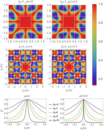
Figure 2: Plots of structure factor $\Sigma_{m}$ obtained from Eq. (17) for $\xi_{0}=0,3,\mu/\epsilon=0,0.3,0.5$ ($k_{x},k_{y}$ in units of $1/a$); $\mu>0$ leads to sharper pinch points even at high $T$. Bottom row: Structure factors cuts on the line $k_{x}=2\pi$ demonstrate discontinuity in the first derivative of the intensity when $\mu>0$.

3. Monopole Interactions and Algebraic Correlations. Consider now $\mu>0$. At small $k$, $\tilde{V}(k)\sim 1/k$ and Eq. (21) reads

$$\overline{\tilde{q}}(k)\simeq\frac{k^{2}}{1+2l_{B}k+\xi_{0}^{2}k^{2}}\frac{Q_{\text{pin}}}{\langle q^{2}\rangle},$$ (22)

which is not analytical at $k=0$, leading to the aforementioned weak singularities at the pinch points. In 3D it would be analytical, because $\tilde{V}(k)\sim~{}1/k^{2}$, the poles of $\overline{\tilde{q}}(k)$ would be purely imaginary [$k_{\pm}=\pm i/\xi_{\text{3D}}$ with $\xi_{\text{3D}}^{-2}=\xi_{0}^{-2}(1+\mu/T)$], and thus $\xi_{\text{3D}}$ would be a screening length. But in 2D the poles are $k_{\pm}=-\bar{k}\pm i/\xi_{\mu}$ with

$$\frac{\xi^{2}_{\mu}}{\xi_{0}^{2}}=\frac{\xi^{2}_{0}}{\xi^{2}_{0}-{l_{B}^{2}}}=\frac{T}{T-T_{\times}}$$ (23)

and they always have a real part $\bar{k}=l_{B}/\xi^{2}_{0}=\mu/2\epsilon$.

Above the crossover temperature $T_{\times}=\mu^{2}/4\epsilon$, $\xi_{0}>l_{B}$, $\xi_{\mu}$ is real, and poles have imaginary parts $i/\xi_{\mu}$. Thus, one could heuristically consider $\xi_{\mu}$ a screening length, and above $T_{\times}$ monopoles are unbound, and the phase is conducive. Below $T_{\times}$, $\xi_{\mu}$ is imaginary, and one could say that there is no screening length, and monopoles are bound by the strength of the magnetic interaction ($\xi_{0}<l_{B}$), in an insulating phase. However, things are more complicated than this naive picture.

In fact, mathematically speaking, there is never a finite screening length. To demonstrate it, consider a charge $Q_{\text{pin}}$ pinned in the origin. From Eqs. (12,13), $\overline{\tilde{V}_{e}}(k)=T\overline{\tilde{q}}(k)/k^{2}$, and thus we obtain

$$\beta\overline{\tilde{V}_{e}}(k)=\frac{\xi_{\mu}}{2i\xi_{0}^{2}}\left(\frac{1}{k-k_{+}}-\frac{1}{k-k_{-}}\right)Q_{\text{pin}}.$$ (24)

Using $2/c=\int_{-\infty}^{\infty}\!\exp(-|z|c)dz$ for $\Re(c)>0$ on each fraction in Eq. (24) and Fourier transforming, we have

$$\beta\overline{V_{e}}(r)=\frac{l_{B}}{2\pi\langle q^{2}\rangle}\int_{-\infty}^{+\infty}\!\!\!\frac{\lambda(z)}{(r^{2}+z^{2})^{3/2}}dz$$ (25)

where $\lambda(z)$ can be interpreted as a linear charge density

$$\lambda(z)=\frac{\xi_{\mu}}{2\xi_{0}^{2}l_{B}}|z|{\sin\left(|z|/\xi_{\mu}\right)}e^{-\bar{k}|z|}Q_{\text{pin}},$$ (26)

for which $\int\lambda(z)dz=Q_{\text{pin}}$. Therefore, the entropic potential can be represented as if generated by a image charge jackson2007classical, spread along a line (of coordinate $z$) perpendicular to the 2D system, and of total charge $Q_{\text{pin}}$.

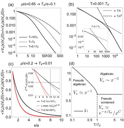
Figure 3: Screening behavior at different $T,\mu$. (a) Log-log plots of the screening entropic potential $\overline{V}_{e}(x)$ (numerically integrated) of Eq. (25) for different temperatures at relatively strong monopole interaction $\mu=0.65\epsilon$ leading to $l\simeq 3$ and $T_{\times}=0.1\epsilon$, where our approximation should still apply. Note the algebraic $~{}1/r^{3}$ decay. However, at high $T$ the potential drops by 99% before becoming algebraic. (b) For $\mu=0.65$ and $T/T_{\times}=10^{-3}$, $\overline{V}_{e}(x)$ shows a pseudo-algebraic decay $\sim 1/r$ for most of its measurable tail (in inset a higher T case, $T/T_{\times}=0.1$). (c) At low monopole interaction ($\mu=0.2\epsilon$) $T_{\times}/\epsilon=0.01$ is very low, most of the charge is screened before the algebraic regime ($l=10$). Effectively, the screening is exponential, and $V_{e}(x)\propto e^{-x/\xi_{\mu}}/x^{0.45}$ provides a good fit (in inset, log plot of $x^{0.45}V_{e}(x)$). (d) Plot of $\bar{k}l$ as a function of $T$ and schematics of the screening at different distances.

Crucially, $\lambda(z)$ is exponentially confined by a length $l$. When $T>T_{\times}$, $l=1/\bar{k}$. When $T<T_{\times}$, the sine in Eq. (26) becomes hyperbolic and $l=1/k_{+}$. For $r\gg l$ the charge is seen as point-like, the potential scales as

$$\overline{V}_{e}(r)\simeq\frac{l_{B}}{2\pi\langle q^{2}\rangle}\frac{Q_{\text{pin}}}{r^{3}},$$ (27)

and, by taking its Laplacian, $\overline{q}(r)$ scales as

$$\overline{q}(r)\simeq-\frac{9l_{B}}{2\pi\langle q^{2}\rangle}\frac{Q_{\text{pin}}}{r^{5}}.$$ (28)

Remarkably, long distance screening—and thus spin correlations—are algebraic at any $T$ (Fig 3a,b). In 3D spin ice, instead, spin correlations are algebraic only at $T=0$, even with monopole interaction. Algebraic screening from a 3D-Coulomb potential in the polarizability of quantum or classical 2D charge systems has been rediscovered multiple times Ando et al. (1982); Keldysh (1979); Jena and Konar (2007); Cudazzo et al. (2011). In fact, it is not merely a 2D feature, but can happen in any dimension for the same dimensional mismatch in the Coulomb interaction Nisoli2020Coulomb.

Figure 4: Heuristic regime diagram. The solid line is $T_{\times}(\mu)$. The dashed line corresponds to 99% of the charge being screened within the radius $l$. On the right of the dotted line, $l\leq 2$ and there is therefore algebraic screening, $\left[\langle q(r)q(0)\rangle\sim r^{-5}\right]$. On the left of the dashed line 99% of the charge is screened within $l$, and, because $T>T_{\times}(\mu)$, the regime is pseudo screened. In the pseudo screened, then algebraic regime the behavior is effectively screened for $x<l$ but more than 1% of the charge is algebraically screened at $x>l$. In the double algebraic region $\langle q(r)q(0)\rangle\sim r^{-3}$ for $x\ll l$ and $\langle q(r)q(0)\rangle\sim r^{-5}$ for $x\gg l$. Note that in nanomagnetic realizations the dumbbell model imposes $\mu/\epsilon<1$.

Importantly, unlike electrical charges, magnetic monopoles are emergent particles of a spin ensemble, and interact entropically. The interplay between the correlation length at zero interaction ($\xi_{0}$) and the Bjerrum length ($l_{B}$) leads to a crossover at $T_{\times}$ between effectively conductive and insulating regimes.

To see that, consider

$$Q_{\text{alg}}/Q_{\text{pin}}\simeq-3l_{B}/\langle q^{2}\rangle l^{3},$$ (29)

the fraction of the charge screened algebraically, obtained by integrating Eq. (28) for $x>l$. When it is very small, and $l$ is large, the algebraic nature of the screening might not be detectable.

When $T\gg T_{\times}$, $|Q_{\text{alg}}/Q_{\text{pin}}|\simeq 10^{-2}$ or less, and thus the algebraic screening might not be experimentally detectable. Moreover, as Fig 3c shows, the screening within $l$ is well fitted by an exponentially screened function. Above $T_{\times}$ there is a “pseudo screening length” $\xi_{\mu}>l_{B}$.

When $T\ll T_{\times}$ we can take $k_{+}\sim 0$ and from Eq. (24) $\overline{\tilde{V}_{e}}(k)\sim 1/k$, and thus $\overline{V}_{e}(r)\sim 1/r$ for $r\ll l=1/k_{+}$ (as confirmed by the numerical plot in Fig 3b). In this regime the insulating phase is easily detectable.

Considering $l$, $T_{\times}$, and $Q_{\text{alg}}$, we can sketch heuristic regime diagrams, which are necessarily somehow arbitrary as they depend on practical specifications. Clearly, when $l$ is smaller than, say, $2$ the behavior is completely algebraic. When $l$ is instead large, there might be pseudo-screening for $x<l$ if $T>T_{\times}$ and if most (we choose 99% in figure) of the charge is screened within a radius $l$ (left side of the dashed line in Fig. 4). If $l\gg 2$ and $Q_{\text{alg}}/Q_{\text{pin}}$ is not small, an initial exponential screening for $r<l$ is followed by algebraic screening for $r\gg l$. Finally, note that $\epsilon$ gets dressed at low temperature. At low $\mu/\epsilon$, the algebraic screening might be extremely hard to detect.

Conclusion. We have developed a field theory for monopoles in degenerate square ice. In absence of a real monopole interaction the system is a 2D-Coulomb gas where monopoles interact entropically, are always screened, and thus in an unbound, conductive phase. This case has been recently realized in quantum dots King et al. (2020). When the 3D-Coulomb interaction among monopoles is considered, reduced dimensionality prevents full screening, and a dimensional mismatch between Green functions of the Laplace operator drive different effective screening regimes.

Our results, obtained via approximations on a simplified mode, invite experimental tests which are however non-trivial: the algebraic behavior can be camouflaged by pseudo-screening if the monopole-monopole interaction is small, and detection might require large real-space characterization. Algebraic correlations might be experimentally detectable in weak singularities near the pinch points, from which the Bjerrum length can be extracted.

In the future, more precise expressions for various quantities can be computed by Feynman diagram expansion of ${\cal F}[\phi]$. The spirit of our approach can be applied also to 3D spin ice and to honeycomb/Kagome spin ice Qi et al. (2008); Zhang et al. (2013), and can be extended to include topological currents beside charges, thus underscoring the gauge-free duality of the square geometry.

References

- Ryzhkin (2005) I. Ryzhkin, Journal of Experimental and Theoretical Physics 101, 481 (2005).
- Castelnovo et al. (2008) C. Castelnovo, R. Moessner, and S. L. Sondhi, Nature 451, 42 (2008).
- Ramirez et al. (1999) A. P. Ramirez, A. Hayashi, R. J. Cava, R. Siddharthan, and B. S. Shastry, Nature 399, 333 (1999).
- den Hertog and Gingras (2000) B. C. den Hertog and M. J. Gingras, Physical review letters 84, 3430 (2000).
- Bramwell and Gingras (2001) S. T. Bramwell and M. J. Gingras, Science 294, 1495 (2001).
- Morris et al. (2009) D. J. P. Morris, D. Tennant, S. Grigera, B. Klemke, C. Castelnovo, R. Moessner, C. Czternasty, M. Meissner, K. Rule, J.-U. Hoffmann, et al., Science 326, 411 (2009).
- Giblin et al. (2011) S. R. Giblin, S. T. Bramwell, P. C. W. Holdsworth, D. Prabhakaran, and I. Terry, Nat. Phys. 7, 252 (2011).
- Kirschner et al. (2018) F. K. Kirschner, F. Flicker, A. Yacoby, N. Y. Yao, and S. J. Blundell, Physical Review B 97, 140402 (2018).
- Henley (2005) C. Henley, Physical Review B 71, 014424 (2005).
- Isakov et al. (2004) S. Isakov, K. Gregor, R. Moessner, and S. Sondhi, Physical Review Letters 93, 167204 (2004).
- Giauque and Stout (1936) W. Giauque and J. Stout, Journal of the American Chemical Society 58, 1144 (1936).
- Bernal and Fowler (1933) J. Bernal and R. Fowler, The Journal of Chemical Physics 1, 515 (1933).
- Pauling (1935) L. Pauling, Journal of the American Chemical Society 57, 2680 (1935).
- Henley (2010) C. L. Henley, Annu. Rev. Condens. Matter Phys. 1, 179 (2010).
- Castelnovo (2010) C. Castelnovo, ChemPhysChem 11, 557 (2010).
- Ladak et al. (2011) S. Ladak, D. Read, W. Branford, and L. Cohen, New Journal of Physics 13, 063032 (2011).
- Mengotti et al. (2010) E. Mengotti, L. J. Heyderman, A. F. Rodríguez, F. Nolting, R. V. Hügli, and H.-B. Braun, Nat. Phys. 7, 68 (2010).
- Zhang et al. (2013) S. Zhang, I. Gilbert, C. Nisoli, G.-W. Chern, M. J. Erickson, L. OB́rien, C. Leighton, P. E. Lammert, V. H. Crespi, and P. Schiffer, Nature 500, 553 (2013).
- Farhan et al. (2019) A. Farhan, M. Saccone, C. F. Petersen, S. Dhuey, R. V. Chopdekar, Y.-L. Huang, N. Kent, Z. Chen, M. J. Alava, T. Lippert, et al., Science advances 5, eaav6380 (2019).
- Tanaka et al. (2006) M. Tanaka, E. Saitoh, H. Miyajima, T. Yamaoka, and Y. Iye, Physical Review B 73, 052411 (2006).
- Wang et al. (2006) R. F. Wang, C. Nisoli, R. S. Freitas, J. Li, W. McConville, B. J. Cooley, M. S. Lund, N. Samarth, C. Leighton, V. H. Crespi, and P. Schiffer, Nature 439, 303 (2006).
- Nisoli et al. (2013) C. Nisoli, R. Moessner, and P. Schiffer, Reviews of Modern Physics 85, 1473 (2013).
- Heyderman and Stamps (2013) L. Heyderman and R. Stamps, Journal of Physics: Condensed Matter 25, 363201 (2013).
- Ortiz-Ambriz et al. (2019) A. Ortiz-Ambriz, C. Nisoli, C. Reichhardt, C. J. Reichhardt, and P. Tierno, Reviews of Modern Physics 91, 041003 (2019).
- Morrison et al. (2013) M. J. Morrison, T. R. Nelson, and C. Nisoli, New Journal of Physics 15, 045009 (2013).
- Bhat et al. (2014) V. Bhat, B. Farmer, N. Smith, E. Teipel, J. Woods, J. Sklenar, J. B. Ketterson, J. Hastings, and L. De Long, Physica C: Superconductivity and its Applications 503, 170 (2014).
- Nisoli (2018) C. Nisoli, in Frustrated Materials and Ferroic Glasses (Springer, 2018) pp. 57–99.
- Skjærvø et al. (2019) S. H. Skjærvø, C. H. Marrows, R. L. Stamps, and L. J. Heyderman, Nature Reviews Physics , 1 (2019).
- Gliga et al. (2019) S. Gliga, G. Seniutinas, A. Weber, and C. David, Materials Today 26, 100 (2019).
- Möller and Moessner (2006) G. Möller and R. Moessner, Phys. Rev. Lett. 96, 237202 (2006).
- Schanilec et al. (2019) V. Schanilec, Y. Perrin, S. L. Denmat, B. Canals, and N. Rougemaille, arXiv preprint arXiv:1902.00452 (2019).
- Perrin et al. (2016) Y. Perrin, B. Canals, and N. Rougemaille, Nature 540, 410 (2016).
- Östman et al. (2018) E. Östman, H. Stopfel, I.-A. Chioar, U. B. Arnalds, A. Stein, V. Kapaklis, and B. Hjörvarsson, Nature Physics 14, 375 (2018).
- King et al. (2020) A. D. King, C. Nisoli, E. D. Dahl, G. Poulin-Lamarre, and A. Lopez-Bezanilla, arXiv preprint arXiv:2007.10555 (2020).
- Kosterlitz and Thouless (1973) J. M. Kosterlitz and D. J. Thouless, Journal of Physics C: Solid State Physics 6, 1181 (1973).
- Borwein et al. (1985) D. Borwein, J. M. Borwein, and K. F. Taylor, Journal of mathematical physics 26, 2999 (1985).
- Lieb (1967) E. H. Lieb, Physical Review 162, 162 (1967).
- Baxter (1982) R. Baxter, Exactly solved models in statistical mechanics (Academic, New York, 1982).
- Nisoli et al. (2010) C. Nisoli, J. Li, X. Ke, D. Garand, P. Schiffer, and V. H. Crespi, Phys. Rev. Lett. 105, 047205 (2010).
- Morgan et al. (2010) J. P. Morgan, A. Stein, S. Langridge, and C. H. Marrows, Nat. Phys. 7, 75 (2010).
- Porro et al. (2013) J. Porro, A. Bedoya-Pinto, A. Berger, and P. Vavassori, New Journal of Physics 15, 055012 (2013).
- Sendetskyi et al. (2019) O. Sendetskyi, V. Scagnoli, N. Leo, L. Anghinolfi, A. Alberca, J. Lüning, U. Staub, P. M. Derlet, and L. J. Heyderman, Physical Review B 99, 214430 (2019).
- Mól et al. (2009) L. Mól, R. Silva, R. Silva, A. Pereira, W. Moura-Melo, and B. Costa, Journal of Applied Physics 106, 063913 (2009).
- Levis et al. (2013) D. Levis, L. F. Cugliandolo, L. Foini, and M. Tarzia, Physical review letters 110, 207206 (2013).
- Nisoli (2020) C. Nisoli, arXiv preprint arXiv:2004.02107 (2020).
- Nisoli (2014) C. Nisoli, New Journal of Physics 16, 113049 (2014).
- Note (1) We denote one-point functions with an overline.
- Garanin and Canals (1999) D. Garanin and B. Canals, Physical Review B 59, 443 (1999).
- Note (2) , with a general function, vertices or edges.
- Castelnovo et al. (2011) C. Castelnovo, R. Moessner, and S. Sondhi, Physical Review B 84, 144435 (2011).
- Chern et al. (2014) G.-W. Chern, C. Reichhardt, and C. Nisoli, Applied Physics Letters 104, 013101 (2014).
- Note (3) Such large values are unattainable in a dumbbell model, thus they are hard to realize in magnetic spin ice.
- Note (4) Low but “not too low”. At really low ordering can take place, as discussed, but also glassy kinetics and non-equilibration.
- Fennell et al. (2009) T. Fennell, P. Deen, A. Wildes, K. Schmalzl, D. Prabhakaran, A. Boothroyd, R. Aldus, D. McMorrow, and S. Bramwell, Science 326, 415 (2009).
- Levin (2002) Y. Levin, Reports on progress in physics 65, 1577 (2002).
- Kaiser et al. (2018) V. Kaiser, J. Bloxsom, L. Bovo, S. T. Bramwell, P. C. Holdsworth, and R. Moessner, Physical Review B 98, 144413 (2018).
- Note (5) Nonetheless, it is possible to show that the state at does belong to the critical portion of the KT transition, and indeed the correlation length is infinite.
- Ando et al. (1982) T. Ando, A. B. Fowler, and F. Stern, Reviews of Modern Physics 54, 437 (1982).
- Keldysh (1979) L. Keldysh, Soviet Journal of Experimental and Theoretical Physics Letters 29, 658 (1979).
- Jena and Konar (2007) D. Jena and A. Konar, Physical review letters 98, 136805 (2007).
- Cudazzo et al. (2011) P. Cudazzo, I. V. Tokatly, and A. Rubio, Physical Review B 84, 085406 (2011).
- Qi et al. (2008) Y. Qi, T. Brintlinger, and J. Cumings, Physical Review B 77, 094418 (2008).