The Dielectric Function of “Astrodust” and Predictions for Polarization in the 3.4$\micron$ and 10$\micron$ Features

Abstract

The dielectric function of interstellar dust material is modeled using observations of extinction and polarization in the infrared, together with estimates for the mass of interstellar dust. The “astrodust” material is assumed to be a mix of amorphous silicates and other materials, including hydrocarbons producing an absorption feature at $3.4\micron$. The detailed shape of the $10\micron$ polarization profile depends on the assumed porosity and grain shape, but the $10\micron$ spectropolarimetric data are not yet good enough to clearly favor one shape over another, nor to constrain the porosity. The expected $3.4\micron$ feature polarization is consistent with existing upper limits, provided the $3.4\micron$ absorption is preferentially located in grain surface layers; a separate population of non-aligned carbonaceous grains is not required. We predict the $3.4\micron$ polarization feature to be $(\Delta p)_{3.4\mu{\rm m}}/p(10\micron)\approx 0.016$, just below current upper limits. Polarization by the same grains at submm wavelengths is also calculated.

1 Introduction

Calculations of absorption, scattering, and emission by interstellar dust particles require assumptions concerning the shapes and sizes of the grains, as well as the dielectric function of the grain material. We have information on the amount of different elements in the grains, as well as observations of the extinction, emission, and polarization properties of the dust at many wavelengths (Hensley & Draine 2020c); these provide some spectroscopic clues to the composition, but at present the detailed composition of the dust remains uncertain.

Some models (e.g. Mathis et al. 1977; Draine & Lee 1984; Weingartner & Draine 2001; Clayton et al. 2003; Zubko et al. 2004; Draine & Fraisse 2009; Compiègne et al. 2011; Jones et al. 2013; Siebenmorgen et al. 2014; Köhler et al. 2015; Siebenmorgen et al. 2017; Fanciullo et al. 2017; Guillet et al. 2018) have idealized interstellar dust as consisting of two or more distinct populations, generally taken to be silicate-rich and carbon-rich materials.

The present paper considers a new model for dust in the diffuse interstellar medium (ISM): the material making up the bulk of the dust is idealized as a mixture of different constituents. For brevity, we refer to this mixed material as astrodust.

The interstellar dust population includes “stardust” particles that were condensed in stellar outflows with a variety of compositions, including silicates, graphite, SiC, Al₂O₃ and other condensates (Nittler & Ciesla 2016). However, in our view the bulk of the interstellar dust material was formed in the cold ISM, by accretion of atoms on grain surfaces in the presence of far-UV radiation; the resulting material is the product of UV photolysis (see, e.g., Draine 2009). The grain size distribution evolves as the result of coagulation in low speed grain-grain collisions, and fragmentation in higher speed collisions. In addition, violent events such as blast waves driven by supernovae occasionally create hostile conditions where much of the solid material may be returned to the gas phase by sputtering, or by vaporization in high velocity grain-grain collisions.

Because we envision the bulk of the grain material as having been grown in the ISM, with large grains having been assembled by coagulation, we idealize grains larger than $\sim$0.02$\micron$ (i.e., the bulk of the interstellar dust mass) as having a mixed composition that is independent of grain size. In addition to these “astrodust” particles, we envision the dust population as also including one or more populations of nanoparticles that individually have distinct composition, such as polycyclic aromatic hydrocarbon (PAH) particles, or nanosilicate particles. Such single-composition nanoparticles may be the result of fragmentation of larger grains in grain-grain collisions.

We estimate below that silicates make up about half of the grain mass. Astrodust is the silicate-bearing grain material, but it includes other compounds, including hydrocarbon material with an absorption feature at 3.4$\micron$. Astrodust material (including voids, if present) will be characterized by an effective dielectric function $\epsilon_{\rm Ad}$. We will estimate $\epsilon_{\rm Ad}$ by requiring that material with this dielectric function reproduce astronomical observations. We consider different assumptions concerning the grain shape and porosity.

There have been previous efforts to characterize the shapes of the silicate-bearing grains. Starlight polarization at optical wavelengths requires that some of the grains be both appreciably nonspherical and substantially aligned (e.g. Kim & Martin 1995). Because polarization is often observed in the $10\micron$ feature (Smith et al. 2000; Whittet 2011), it is clear that the silicate-bearing grains must be significantly nonspherical and aligned. Draine & Lee (1984) and Lee & Draine (1985) argued that the polarization profile of the 10$\micron$ feature towards the Becklin-Neugebauer (BN) object favored oblate grain shapes, and Aitken et al. (1989) reached the same conclusion. However, the grains in the diffuse ISM may differ from those obscuring the BN object. Some recent studies focusing on submm polarization (e.g., Siebenmorgen et al. 2017; Guillet et al. 2018) favored prolate shapes for the grains in the diffuse ISM, but did not address the 10$\micron$ silicate feature.

Figure 1: Approach used to determine the shape and dielectric function $\epsilon_{\rm Ad}$ of the silicate-bearing “astrodust” grains. ${\cal P}$ is the porosity of the astrodust grains (see text).

The present paper uses the most accurate available observations of infrared absorption and polarization by dust, summarized in §3, to try to constrain the shape, porosity, and dielectric function $\epsilon_{\rm Ad}$ of the silicate-bearing grains in the diffuse ISM. Our approach (outlined in Figure 1) consists of testing different hypotheses for shape and porosity by using the observed interstellar absorption (§3) and estimates of the volume of astrodust material (see §4) to solve for a self-consistent effective dielectric function $\epsilon_{\rm Ad}(\lambda)$ (see §5). Having found $\epsilon_{\rm Ad}(\lambda)$, we then calculate the 10$\micron$ polarization; comparison of the model polarization to published spectropolarimetry of the 10$\micron$ silicate feature (§6) favors some shapes over others. Predicted polarization at other wavelengths ($3.4\micron$ feature; far-infrared and submm) is discussed in §7.

Our results are discussed in §8, and summarized in §9. Various technical points are examined in Appendices A – C.

2 Motivation for a One-Component Model

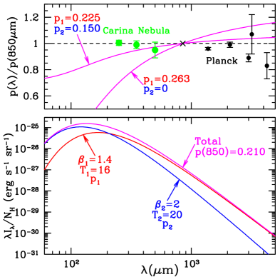
Figure 2: Upper panel: Symbols: polarization, relative to $p(850\micron)$, measured by Planck (Planck Collaboration et al. 2015b) for the general ISM, and BLASTPol (Shariff et al. 2019) for the Carina Nebula. Curves: two-component toy model (see text), with two different choices for the component polarizations $p_{1}$ and $p_{2}$. Even with $p_{1}/p_{2}=1.5$, the wavelength-dependence of $p(\lambda)$ appears to be inconsistent with observations. Lower panel: emission spectra for the two-component toy model (see text). The toy model emission spectrum peaks near $140\micron$, and is broadly consistent with $\lambda\geq 60\micron$ observations of the diffuse ISM.

Many models of interstellar dust have postulated the existence of two major components: silicate dust and carbonaceous dust, with the two grain types having similar size distributions, and similar total volumes of material (e.g., Mathis et al. 1977). Such models appeared to be compatible with observations of wavelength-dependent extinction and starlight polarization, and seemed to be favored because of nondetection of polarization in the $3.4\micron$ CH feature on sightlines where the $10\micron$ silicate feature is appreciably polarized (Chiar et al. 2006), which could be explained if for some reason the carbonaceous grains are not aligned.

At far-infrared and submm wavelengths, the fractional polarization $p$ of the thermal emission from a single grain is expected to be nearly independent of wavelength. Because the two dust components are likely to be heated to different temperatures by starlight, to have different wavelength-dependences for their far-infrared (FIR) and submm opacities, and to have different shapes and degrees of alignment, two-component models naturally predict that the fractional polarization of the FIR and submm emission will vary with wavelength (Draine & Fraisse 2009). To illustrate this, Figure 2 shows the polarization fraction $p(\lambda)$ at $\lambda>60\micron$ for a simple two-component toy model, where the two components have slightly different temperatures, opacities $\propto\nu^{\beta}$ with different values of $\beta$, and polarization fractions $p_{1}$ and $p_{2}$. The toy model shown has $T_{1}=16\,{\rm K}$ and $T_{2}=20\,{\rm K}$, and $\beta_{1}=1.4$ and $\beta_{2}=2$. If the two components contribute approximately equally at $200\micron$, the overall emission for this model approximates the observed spectral energy distribution (SED) of the diffuse ISM (see, e.g., Hensley & Draine 2020c). However, unless the two components each have identical fractional polarizations (i.e., $p_{1}=p_{2}$), the overall polarization fraction will be frequency dependent. The extreme case where only component 1 is polarized is illustrated in Figure 2, resulting in a total polarization fraction that varies by a factor of $\sim$$1.7$ from $250\micron$ to $3\,{\rm mm}$. We also show an example with $p_{1}/p_{2}=1.5$. For this example, $p(\lambda)$ varies by a factor of $\sim$$1.13$ from $250\micron$ to $3\,{\rm mm}$.

Planck found the fractional polarization to be essentially constant for $\lambda\geq 850\micron$ (Planck Collaboration et al. 2015b). BLASTPol (Ashton et al. 2018; Shariff et al. 2019) measured the polarization fraction to be nearly constant for $250\micron\leq\lambda\leq 850\micron$ in selected brighter areas (see Figure 2). The toy model examples shown in Figure 2 are inconsistent with these observations. In order to make a two-component model work, one requires that either (1) the two components have very similar SEDs, or (2) the two components have nearly identical fractional polarizations. If the two grain types are actually quite dissimilar (e.g, silicate grains and carbon grains), one would expect the two components to have different SEDs, and different polarized fractions.

If, however, a single grain type dominates the FIR-submm emission, then it is natural for the polarization fraction to be nearly frequency-independent at long wavelengths. This is the type of model considered here.

3 Infrared Absorption by Interstellar Dust

The observed extinction produced by dust in the ISM is discussed by Hensley & Draine (2020c). At wavelengths $\lambda\lesssim 30\micron$ the extinction is obtained from the observed attenuation on sightlines to stars. In the near-IR ($1-8\micron$) numerous sightlines have been studied, using observations from the ground and space, including the IRAC camera on Spitzer Space Telescope and WISE (e.g., Indebetouw et al. 2005; Schlafly et al. 2016). At longer wavelengths, sightlines with very large dust columns are required to accurately measure the extinction. The 8–30$\micron$ extinction curve that we use here is based on a reanalysis of archival Spitzer IRS data for the star Cyg OB2-12 (Hensley & Draine 2020b).

At wavelengths $\lambda\gtrsim 50\micron$, the attenuation is very weak and has not been measured directly, but the absorption produced by interstellar dust can be inferred from the observed thermal emission. The resulting extinction cross section per H for astrodust in the general diffuse ISM at intermediate to high galactic latitudes, $\tau_{\rm ext}/N_{\rm H}$, is shown in Figure 3 for $\lambda>1\micron$ (Hensley & Draine 2020b, c).

PAH nanoparticles are expected to contribute infrared extinction features at 3.3, 6.2, and 7.7$\micron$; absorption features at these wavelengths are observed (Schutte et al. 1998; Chiar et al. 2000; Hensley & Draine 2020b) and have been subtracted from the observed extinction to obtain the astrodust-only extinction shown in Figure 3. In addition to the prominent silicate features at 9.7$\micron$ and 18$\micron$, the astrodust extinction includes absorption features at $3.4\micron$ and $6.85\micron$ due to aliphatic hydrocarbons; these are shown in Fig. 4. The interstellar $3.4\micron$ CH absorption feature is composed of subfeatures contributed by aromatic, aliphatic, and diamond-like hydrocarbons (Chiar et al. 2013; Hensley & Draine 2020b). PAH nanoparticles are expected to contribute to the “aromatic CH” absorption component at $3.29\micron$, and may well be responsible for the bulk of the $3.29\micron$ absorption feature. Because we don’t know what fraction of the $3.29\micron$ extinction feature to attribute to aromatic material in the astrodust component, we obtain a lower bound on the astrodust absorption by subtracting the entire $3.29\micron$ aromatic component from the observed extinction, leaving only the contributions from aliphatic or diamondlike hydrocarbons in the profile shown in Fig. 4a.

In this work we seek to estimate the complex dielectric function for interstellar dust. When particles are small compared to the wavelength (i.e., in the Rayleigh limit), extinction is dominated by absorption; the absorption cross section per grain volume $C_{\rm abs}/V$ is then directly related to the complex dielectric function $\epsilon_{\rm Ad}(\lambda)$, and is independent of the grain size $a$.

According to models that reproduce the observed reddening in diffuse regions (e.g., Mathis et al. 1977; Weingartner & Draine 2001) the extinction at wavelengths $\lambda\gtrsim 3\micron$ in the diffuse ISM is dominated by absorption: scattering makes only a minor contribution. For example, the $R_{V}=3.1$ grain model of Weingartner & Draine (2001) has albedo $<0.05$ at $\lambda>7\micron$. At wavelengths $\lambda\geq 8\micron$ where scattering is minimal, it may be safely assumed that interstellar grains are in the Rayleigh limit $a\ll\lambda$. At shorter wavelengths, we take the “Rayleigh limit” absorption per H to be a wavelength-dependent fraction of the extinction. Figure 3 shows our estimate for the dust absorption per H nucleon in the Rayleigh limit.

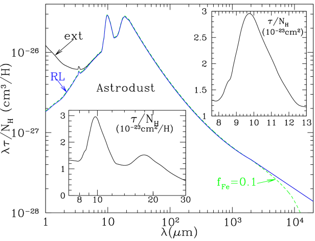
Figure 3: Solid black curve: $\lambda\tau_{\rm ext}/N_{\rm H}$ for $\lambda>1\micron$, where $\tau_{\rm ext}/N_{\rm H}$ is the observed extinction cross section per H nucleon at intermediate and high galactic latitudes at wavelength $\lambda$ (from Hensley & Draine 2020b). Extinction in the PAH features is not included. The blue curve (RL) shows our estimate for $\lambda\tau_{\rm abs}/N_{\rm H}$ if the grains were all in the Rayleigh limit. The green broken curve shows the reduced level of electric dipole absorption required if there is magnetic dipole absorption provided by a fraction $f_{\rm Fe}=0.1$ of the Fe in metallic inclusions. Insets show details of the 9.7 and 18$\micron$ silicate features.

Figure 4: Astrodust hydrocarbon absorption features (see text) at 3.4$\micron$ and $6.85\micron$ based on sightline to Cyg OB2-12 (Hensley & Draine 2020b). The $3.29\micron$ aromatic absorption feature has been removed.

The complex dielectric function $\epsilon_{\rm Ad}(\omega)$ characterizes the response of the grain material to applied electric fields, and therefore does not include any magnetic absorption. If a fraction $f_{\rm Fe}$ of the iron is present in the form of metallic Fe inclusions, these will provide strong magnetic absorption at frequencies $\nu<100\,{\rm GHz}$, or wavelengths $\lambda>3\,{\rm mm}$ (Draine & Hensley 2013), and will contribute to the thermal emission at these frequencies. If the metallic Fe fraction $f_{\rm Fe}>0$, we estimate the magnetic absorption as described in Appendix A. The magnetic dipole contribution to the absorption is then subtracted from the observed opacity to yield the electric contribution to the absorption. Figure 3 shows our estimate for the electric dipole absorption at long wavelengths for $f_{\rm Fe}=0$ and 0.1. For $f_{\rm Fe}\lesssim 0.2$, the magnetic contribution to absorption is significant only at very long wavelengths ($\lambda\gtrsim 5\,{\rm mm}$, $\nu\lesssim 60\,{\rm GHz}$).

4 Abundance of Materials in Interstellar Grains

In diffuse regions that have been probed by ultraviolet spectroscopy, we can estimate the total grain mass by summing up the atoms and ions observed in the gas phase and subtracting this sum from our best estimate for the total elemental abundances in the diffuse ISM. With reasonable assumptions for the mass densities of the materials containing the missing atoms, we can then estimate the volume of solid material.

Jenkins (2009) studied variations in gas-phase abundances, finding that the gas-phase abundances in a single cloud can be predicted using a single “depletion parameter” $F_{\star}$ that characterizes the overall level of depletion (sequestration of elements into solid grains) in that cloud. In Jenkins’s sample, the median sightline had $F_{\star}\approx 0.5$, which we take to be representative of diffuse H I.

Table 1: Elemental Abundances in Gas and Dust (ppm) (Hensley & Draine 2020c)

$X$	$(X/{\rm H})_{\rm ISM}$	$(X/{\rm H})_{\rm gas}$	$(X/{\rm H})_{\rm dust}$
C	324	198	126
O	682	434	248
Mg	52.9	7.1	46
Al	3.48	0.07	3.4
Si	44.6	6.6	38.0
S	17.2	9.6	7.6
Ca	3.25	0.07	3.2
Fe	43.7	0.9	43
Ni	2.09	0.04	2.1

Table 2: Nominal Composition of astrodust Grains

$f_{\rm Fe}=$	0	0.10
species	(ppm relative to H)
Mg1.3(Fe,Ni)0.3SiO3.6 ($\rho=3.41\,{\rm g}\,{\rm cm}^{-3}$)	35.4	35.4
(Fe,Ni) metal ($\rho=7.9\,{\rm g}\,{\rm cm}^{-3}$)	0	4.5
(Fe,Ni)3O4 ($\rho=5.15\,{\rm g}\,{\rm cm}^{-3}$)	8.9	7.4
(Fe,Ni)S ($\rho=4.84\,{\rm g}\,{\rm cm}^{-3}$)	7.6	7.6
CaCO3 ($\rho=2.71\,{\rm g}\,{\rm cm}^{-3}$)	3.2	3.2
Al2O3 ($\rho=4.02\,{\rm g}\,{\rm cm}^{-3}$)	1.7	1.7
SiO2 ($\rho=2.20\,{\rm g}\,{\rm cm}^{-3}$)	2.8	2.8
C (in hydrocarbons, $\rho\approx 2\,{\rm g}\,{\rm cm}^{-3}$)	83.	83.
C in PAH nanoparticles	40.	40.
O unaccounted for	66.	70.
volume estimates
$V_{\rm sil}[10^{-27}\,{\rm cm}^{3}{\rm H}^{-1}]$	2.31	2.31
$V_{\rm mix}[10^{-27}\,{\rm cm}^{3}{\rm H}^{-1}$	1.29	1.18
$V_{\rm car}[10^{-27}\,{\rm cm}^{3}{\rm H}^{-1}]$	0.86	0.86
$V_{\rm Fe}[10^{-27}\,{\rm cm}^{3}{\rm H}^{-1}]$	0.	0.053
$V_{\rm Ad}(1-{\cal P})\,\,[10^{-27}\,{\rm cm}^{3}{\rm H}^{-1}]$	4.46	4.40
$\rho_{\rm Ad}/(1-{\cal P})\,\,[\,{\rm g}\,{\rm cm}^{-3}]$	3.42	3.43
mass estimates
Astrodust:
silicate mass/H mass	0.0047	0.0047
(Fe,Fe3O4,FeS)/H mass	0.0027	0.0026
carbon mass/H mass	0.0010	0.0010
(Al2O3,CaCO3,SiO2)/H mass	0.0007	0.0007
total astrodust mass/H mass	0.0092	0.0091
PAH mass/H mass	0.0005	0.0005
Total grain mass/H mass	0.0097	0.0096

Estimates for the gas-phase abundances $(X/{\rm H})_{\rm gas}$ are given in Table 1 for $X=$ C, O, Mg, Si, S, Al, Ca, Fe, and Ni in diffuse regions with $F_{\star}=0.5$. Table 1 also lists interstellar abundances $(X/{\rm H})_{\rm ISM}$ recommended by Hensley & Draine (2020c); using these values we obtain $(X/{\rm H})_{\rm dust}=(X/{\rm H})_{\rm ISM}-(X/{\rm H})_{\rm gas}$ recommended by Hensley & Draine (2020c), shown again in Table 1.

We model the interstellar dust population as separate populations of (1) astrodust grains, containing the bulk of the dust mass; and (2) $a\lesssim 0.01\micron$ nanoparticles, including PAHs. We assume the astrodust material to be a mixture of different components: (1) silicates, (2) a mixture of other compounds of Fe, Si, S, Al, Ca, etc., (3) carbonaceous material, and, possibly, (4) metallic Fe-Ni inclusions.

Let $V_{\rm Ad}$ be the astrodust volume/H. If astrodust grains include a volume fraction ${\cal P}$ of vacuum, then

$$(1-{\cal P})V_{\rm Ad}=V_{\rm sil}+V_{\rm mix}+V_{\rm car}+V_{\rm Fe\,inc}~{},$$ (1)

where $V_{\rm sil}$, $V_{\rm mix}$, $V_{\rm car}$, and $V_{\rm Fe\,inc}$, are, respectively, the solid volume per H of the silicate material, other non-silicate materials, carbonaceous material, and the metallic Fe-Ni inclusions.

4.1 Mg and Si

The elemental composition of the interstellar silicate material remains uncertain, but evidence points to a Mg-rich composition intermediate between pyroxenes and olivines. Based on the profile of the $10\micron$ silicate feature, Min et al. (2007) favored a model with overall silicate composition Mg_1.32Fe_0.10SiO_3.45. Studies of the extinction profiles of the 10 and 18$\micron$ features toward $\zeta$Oph led Poteet et al. (2015) to favor a silicate mixture with overall composition Mg_1.48Fe_0.32SiO_3.79. Fogerty et al. (2016) fit the silicate profile toward Cyg OB2-12 with a silicate mixture having overall composition Mg_1.37Fe_0.18Ca_0.002SiO_3.55. We adopt a nominal silicate composition Mg_1.3(Fe,Ni)_0.3SiO_3.6, for which we estimate a density $\rho=3.41\,{\rm g}\,{\rm cm}^{-3}$.

For the adopted nominal composition Mg_1.3(Fe,Ni)_0.3SiO_3.6 and the abundances $(X/{\rm H})_{\rm dust}$ in Table 1, Mg is the limiting constituent. The interstellar $9.7\micron$ silicate absorption feature is strong; we will assume 100% of the Mg in grains to be in silicates. We estimate the amorphous silicate volume to be

$$V_{\rm sil} = 2.32{\!\,\times\!\,}10^{-27}\,{\rm cm}^{3}{\rm H}^{-1}~{}.$$ (2)

4.2 Fe

The fraction $f_{\rm Fe}$ of the solid-phase Fe that is in metallic form is difficult to constrain directly, because metallic Fe lacks spectral features in the IR. However, metallic Fe is ferromagnetic, and would generate thermal magnetic dipole emission with unusual spectral and polarization characteristics (Draine & Hensley 2013). We treat $f_{\rm Fe}$ as an unknown parameter, but we consider it likely to be small in the local ISM, $f_{\rm Fe}\lesssim 0.1$.

For the assumed silicate composition Mg_1.3(Fe,Ni)_0.3SiO_3.6, $\sim$25% of the (Fe,Ni) is in the silicate material; thus $f_{\rm Fe}\lesssim 0.75$. The volume contributed by Fe-Ni metallic inclusions (density $\rho=7.9\,{\rm g}\,{\rm cm}^{-3}$) is

$$V_{\rm Fe\,inc}=5.3f_{\rm Fe}{\!\,\times\!\,}10^{-28}\,{\rm cm}^{3}{\rm H}^{-1}~{}~{}.$$ (3)

Candidate materials for the remaining Fe include oxides (FeO, Fe₃O₄, Fe₂O₃, …), carbides (Fe₃C, …), and sulfur compounds (FeS, FeS₂, FeSO₄, …). Nondetection of absorption features at 22$\micron$ and 16$\micron$ imposes upper limits on the abundances of FeO and Fe₃O₄ toward $\zeta$Oph (Poteet et al. 2015) and Cyg OB2-12 (Hensley & Draine 2020b) but still allows a significant fraction of the Fe to be in each of these species. At this time the chemical form of $\sim$75% of the Fe is unknown.

4.3 Carbon

About 126 ppm of C is missing from gas with $F_{\star}=0.5$ (see Table 1). We estimate that $\sim$40 ppm of C is contained in PAH nanoparticles that account for the observed PAH emission features, as well as the prominent 2175Å extinction feature. We assume the remainder of the solid-phase carbon to be in the astrodust, with 3 ppm in CaCO₃ and the remainder in hydrocarbons . Assuming the hydrocarbon material to have C:H $\sim$ 2:1, and C mass density $\rho_{\rm C}=2\,{\rm g}\,{\rm cm}^{-3}$, the hydrocarbon volume in the silicate-bearing grains is

$$V_{\rm hc} \,=\, 8.3\times 10^{-28}\,{\rm cm}^{3}{\rm H}^{-1}~{}~{}.$$ (4)

4.4 Other

As noted above, there may be a significant amount of Fe that is not in silicates and not metallic Fe. S, Al, and Ca are also present in the grains, although with abundances small compared to Mg, Si, and Fe (see Table 1). To estimate the volume $V_{\rm mix}$ of non-silicate, non-carbonaceous, material (not including metallic Fe), we suppose that the small fraction ($\sim$10%) of the Si that is not in silicates is in SiO₂ ($\rho=2.2\,{\rm g}\,{\rm cm}^{-3}$), the Ca is in CaCO₃ ($\rho=2.71\,{\rm g}\,{\rm cm}^{-3}$), the Al is in Al₂O₃ ($\rho=4.0\,{\rm g}\,{\rm cm}^{-3}$), the S is in (Fe,Ni)S ($\rho=4.8\,{\rm g}\,{\rm cm}^{-3}$) and the remaining (Fe,Ni) atoms are in a mixture of oxides (Fe₂O₃, Fe₃O₄, FeO) with overall ratio O:(Fe,Ni)::4:3 and density as for magnetite Fe₃O₄ ($\rho=5.2\,{\rm g}\,{\rm cm}^{-3}$) . This mixture contributes a volume per H

$$V_{\rm mix} \,=\, 1.29(1-0.78f_{\rm Fe}){\!\,\times\!\,}10^{-27}\,{\rm cm}^{3}{\rm H}^{-1}~{}.$$ (5)

The astrodust volume is

$$V_{\rm Ad} \,=\, \frac{4.46{\!\,\times\!\,}10^{-27}\,{\rm cm}^{3}{\rm H}^{-1}}{(1-{\cal P})}\times\left(1-0.22f_{\rm Fe}\right)~{}.$$ (6)

The fraction of the solid volume contributed by the metallic Fe nanoparticles is

$$f_{\rm sv,Fe}\equiv\frac{V_{\rm Fe\,inc}}{(1-{\cal P})V_{\rm Ad}}\approx\frac{0.12f_{\rm Fe}}{1-0.22f_{\rm Fe}}~{}.$$ (7)

For $f_{\rm Fe}\lesssim 0.1$, the volume fraction of metallic Fe is small, $f_{\rm sv,Fe}\lesssim 0.01$. The fraction of the solid volume contributed by the silicate material itself is

$$\frac{V_{\rm sil}}{V_{\rm sil}+V_{\rm mix}+V_{\rm car}+V_{\rm Fe\,inc}}\approx\frac{0.52}{1-0.22f_{\rm Fe}}~{}.$$ (8)

4.5 The Oxygen Problem

Jenkins (2009) pointed out that in diffuse regions with average depletions, there does not appear to be a plausible candidate material to incorporate the oxygen that is missing from the gas (Whittet 2010). In diffuse regions, H₂O ice is not detected, and cannot account for the missing oxygen. The adopted astrodust composition accounts for only

$$\left(\frac{\rm O}{\rm H}\right)_{\rm dust} \,\approx\, (183-54f_{\rm Fe}){\rm ppm}~{},$$ (9)

Comparing to Table 1, we see that $\sim$66 ppm of oxygen – 10% of the total – appears to be unaccounted for in regions where $F_{\star}=0.5$. Upper limits on the $3.1\micron$ feature imply that the missing oxygen cannot be attributed to H₂O ice in submicron grains (Poteet et al. 2015). The “missing oxygen” remains unexplained.

4.6 Dust Volume per H

Table 2 lists the contributions of each of the materials to the grain volume. The density of the astrodust mixture is $\rho_{\rm Ad}=3.42(1-{\cal P})\,{\rm g}\,{\rm cm}^{-3}$ (for $f_{\rm Fe}=0$). With the abundances in Table 1, the dust/H mass ratio is $0.0097$.

4.7 Elemental Abundances in the Diffuse ISM

Many discussions of dust abundances in the ISM implicitly assume that the local ISM is vertically well-mixed, with the same overall elemental abundances both near the midplane as well as in the more diffuse ISM above and below the plane. Because elements such as Mg, Si, and Fe are heavily depleted even in diffuse regions characterized by depletion parameter $F_{\star}\approx 0.5$ (see Table 1), this would lead to the expectation that the dust/gas ratio would be nearly the same in all diffuse H I and H₂ clouds, because the additional depletion taking place in dense regions adds very little Mg, Si, and Fe to the dust.

Using H Lyman $\alpha$ and ${\rm H}_{2}$ Lyman and Werner band lines to measure $N_{\rm H}=N({\rm H})+2N({\rm H}_{2})$ on sightlines to O and B stars, Bohlin et al. (1978) found $\langle E(B-V)/N_{\rm H}\rangle=1.7\times 10^{-22}\,{\rm cm}^{2}{\rm H}^{-1}$ and Diplas & Savage (1994) obtained $\langle E(B-V))/N_{\rm H}\rangle=(2.03\pm 0.12)\times 10^{-22}\,{\rm cm}^{2}{\rm H}^{-1}$. For many years these were taken to be canonical values for the local ISM.

However, more recent studies of high latitude H I gas have found significantly less reddening per H: $\langle E(B-V)/N_{\rm H}\rangle\approx(1.12\pm 0.1)\times 10^{-22}\,{\rm cm}^{2}{\rm H}^{-1}$ (Lenz et al. 2017) and $(1.1\pm 0.2)\times 10^{-22}\,{\rm cm}^{2}{\rm H}^{-1}$ (Nguyen et al. 2018). We take this to indicate that the abundances relative to H of the dust-forming elements vary, with enhanced abundances near the midplane. Because gravity causes dust grains to drift systematically toward the midplane, an enhancement in the abundances of the dust-forming elements is anticipated, although the expected magnitude of the enhancement is highly uncertain, depending on the competition between gravitationally-driven settling versus mixing by vertical motions, including turbulence.

Our knowledge of the abundances of the dust-forming elements derives from measurements of elemental abundances in stellar atmospheres, which reflect the abundances of dust and gas in the gas cloud where the star formed. Because star formation occurs preferentially in dense regions near the midplane, the abundances in a stellar atmospheres are, effectively, the mid-plane abundances in the ISM at the time the star formed. The dust solid volume per H $V_{\rm Ad}(1-{\cal P})=4.46\times 10^{-27}\,{\rm cm}^{3}{\rm H}^{-1}$ in Table 2 is based on measured abundances in stars, and therefore should give the dust volume per H in midplane regions.

Our estimate of the far-infrared opacity per H is based on observations of H I-correlated FIR and submm emission at intermediate and high galactic latitudes. As discussed above, the dust-to-gas ratio in this gas is expected to be lower than in the mid-plane regions.

Let $V_{\rm Ad,hgl}$ be the volume of astrodust grains per H nucleon in diffuse H I at intermediate or high galactic latitudes (i.e., away from the midplane). With $E(B-V)/N_{\rm H}\approx 1.1\times 10^{-22}\,{\rm cm}^{2}{\rm H}^{-1}$ in high-latitude gas only $\sim$$2/3$ of $E(B-V)/N_{\rm H}\approx 1.9\times 10^{-22}\,{\rm cm}^{2}{\rm H}^{-1}$ near the mid-plane, we adopt

$$V_{{\rm Ad,hgl}}=\frac{3.0{\!\,\times\!\,}10^{-27}}{(1-{\cal P})}\left(1-0.22f_{\rm Fe}\right)\,{\rm cm}^{3}\,{\rm H}^{-1}~{}~{},$$ (10)

i.e., about $2/3$ of the value given in Table 2.

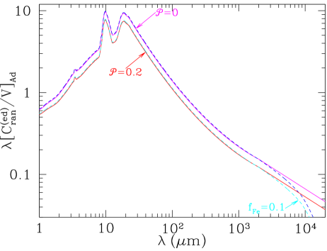
Figure 5: Assumed $\lambda[C_{\rm ran}^{\rm(ed)}/V]_{\rm Ad}$, where $[C_{\rm ran}^{\rm(ed)}/V]_{\rm Ad}$ is the absorption cross section per unit grain volume for randomly-oriented astrodust grains in the electric dipole limit, for porosity ${\cal P}=0$, and 0.2 and $f_{\rm Fe}=0$ and 0.1 .

4.8 Astrodust Absorption Per Unit Grain Volume vs. $\lambda$

Except for a small contribution to the mid-IR extinction from PAH nanoparticles, we require that astrodust grains reproduce the entire observed interstellar extinction for $\lambda>1\micron$. Because the porosity of astrodust is not known, we consider a range of porosities $0\leq{\cal P}\leq 0.9$.

The astrodust cross section per unit volume

$$(C/V)_{\rm Ad}=\frac{(\tau/N_{\rm H})_{\rm hgl}}{V_{\rm Ad,hgl}}~{}~{}.$$ (11)

Figure 5 shows our estimate for $[C_{\rm abs}^{\rm(ed)}/V]_{\rm Ad}$, the absorption per volume in the electric dipole limit, at $\lambda\geq 1\micron$, for two values of ${\cal P}$ and two values of $f_{\rm Fe}$. Note that varying $f_{\rm Fe}$ from 0 to 0.1 only changes $C_{\rm abs}^{\rm(ed)}/V$ noticeably for $\lambda\gtrsim 5\,{\rm mm}$ ($\nu\lesssim 60\,{\rm GHz}$).

5 Effective Dielectric Function

We seek a self-consistent effective complex dielectric function $\epsilon_{\rm Ad}(\lambda)$ for astrodust that satisfies the observational constraints. This effective dielectric function $\epsilon_{\rm Ad}(\lambda)$ characterizes the overall response of the grain interior, including the silicate material, vacuum, and other materials present within an assumed spheroidal or ellipsoidal surface. The derived $\epsilon_{\rm Ad}(\lambda)$ depends on three separate assumptions:

1. The grain shape (we consider either spheroids with specified axis ratio $b/a$, or certain continuous distributions of ellipsoids);

2. ${\cal P}=$ fraction of the astrodust grain volume that is occupied by vacuum;

3. $f_{\rm Fe}=$ fraction of the interstellar Fe that is in the form of metallic Fe inclusions.

The derived $\epsilon_{\rm Ad}(\lambda)$ is intended to describe the material in the astrodust grains at wavelengths from microwaves to X-rays. We separate the dielectric function into two components:

$$\epsilon_{\rm Ad}-1=(\epsilon_{\rm Ad}^{\rm ox}-1)+(\epsilon_{\rm Ad}^{\rm ir}-1)~{}~{},$$ (12)

where the “optical through X-ray” component ${\rm Im}(\epsilon_{\rm Ad}^{\rm ox})$ accounts for absorption at $\lambda<1\micron$, and ${\rm Im}(\epsilon_{\rm Ad}^{\rm ir})$ describes absorption at $\lambda\geq 1\micron$. We “solve” for $\epsilon_{\rm Ad}^{\rm ir}$ by adjusting it to comply with observational constraints on absorption at wavelengths $\lambda>1\micron$.

The procedure for obtaining ${\rm Im}\left(\epsilon_{\rm Ad}^{\rm ox}\right)$ is described in Appendix B. In brief, we obtain the “optical through X-ray” dielectric function $\epsilon_{\rm mat}^{\rm ox}$ for the astrodust material, with no voids and no Fe inclusions, using general considerations for how absorptive astrodust material is thought to be at wavelengths $\lambda<1\micron$. This dielectric function provides a level of absorption at optical wavelengths that appears to be consistent with the observed absorption of starlight by interstellar dust, and includes a rapid rise in the absorption shortward of $\sim$$0.15\micron$ due to the onset of interband absorption. The adopted ${\rm Im}\left(\epsilon_{\rm Ad}^{\rm ox}\right)$ is consistent with oscillator strength sum rules for the assumed dust elemental composition. For each adopted ${\cal P}$ and $f_{\rm Fe}$, we then use effective medium theory to obtain $\epsilon_{\rm Ad}^{\rm ox}$ from $\epsilon_{\rm mat}^{\rm ox}$.

To model the infrared absorption, we take

$$\epsilon_{\rm Ad}^{\rm ir}(\omega)-1=\sum_{k=1}^{N}\frac{S_{k}}{\left[1-\left(\omega/\omega_{k}\right)^{2}-i\gamma_{k}\left(\omega/\omega_{k}\right)\right]}~{}~{}~{},$$ (13)

using $N=3000$ damped Lorentz oscillators, with resonant frequencies $\omega_{k}$ distributed between $\omega_{1}=2\pi c/1\micron$ and $\omega_{N}=2\pi c/5\,{\rm cm}$, and suitably chosen fractional widths $\gamma_{k}$ (see Draine & Hensley 2017). The $\omega_{k}$ are uniformly-distributed in $\ln(\omega)$ between $\lambda_{1}=1\micron$ and $\lambda_{2000}=100\micron$, with a smooth transition to wider spacing in $\ln(\omega)$ at longer wavelengths. The broadening parameters are taken to be

$$\gamma_{k} = C\left(\frac{\omega_{j-1}}{\omega_{j}}-1\right)~{}~{}~{},~{}~{}~{}j=\max(2,k)~{}~{}~{}.$$ (14)

For $C=10$ the overlap between resonances yields a dielectric function that is sufficiently smooth for our purposes, with individual oscillators having sufficiently narrow resonances to be able to represent a dielectric function that varies relatively rapidly in the vicinity of the $9.7\micron$ Si-O profile.

With the frequencies and widths of the resonances specified, the strengths $S_{k}$ remain to be determined. Individual $S_{k}$ are allowed to be negative – it is only necessary that ${\rm Im}(\epsilon_{\rm Ad})>0$ after summing over the contributions from all of the oscillators plus ${\rm Im}(\epsilon^{\rm ox})$. The $S_{k}$ are obtained by requiring that the resulting dielectric function $\epsilon_{\rm Ad}$ reproduce the $[C_{\rm ran}^{\rm(ed)}/V]_{\rm Ad}$ consistent with the observed extinction and emission – see Figure 5.

We consider spheroidal grains with a wide range of possible axis ratios, from prolate shapes with $b/a$ as small as $1/3$, to oblate shapes with $b/a=3$. We also consider ellipsoidal grains with two different continuous distributions of ellipsoidal shapes:

1. The shape distribution proposed by Ossenkopf et al. (1992), referred to as “CDE2” by Fabian et al. (2001).

2. The “externally-restricted CDE” (ERCDE) distribution (Zubko et al. 1996) with $L_{\rm min}=0.05$, i.e., restricted to shape factors $0.05\leq L\leq 0.9$.

Properties of these two shape distributions are discussed in Draine & Hensley (2017). Although the continuous distribution of ellipsoids (CDE) discussed by Bohren & Huffman (1983) is often used (e.g., Rouleau & Martin 1991; Alexander & Ferguson 1994; Min et al. 2003, 2008) we do not employ it here, because we do not consider it to be realistic. The Bohren-Huffman CDE distribution includes a large fraction of extremely elongated or flattened shapes – fully 10% of Bohren-Huffman CDE ellipsoids have axis ratios $a_{3}/a_{1}>20$, and 1% have $a_{3}/a_{1}>100$ (Draine & Hensley 2017). Such extreme elongations seem to us to be unlikely, therefore the present study considers only the ERCDE and CDE2 shape distributions.

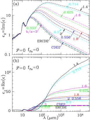
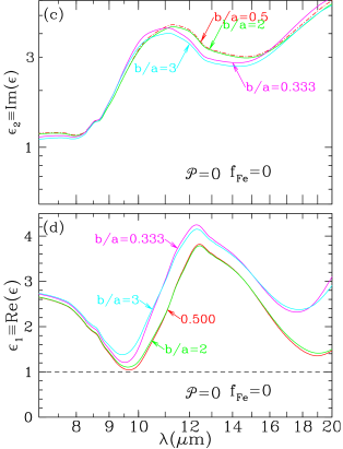
Figure 6: (a,b): ${\rm Im}(\epsilon)$ and ${\rm Re}(\epsilon)$. (c,d): expanded view of 7–20$\micron$ region. Results are shown for ${\cal P}=0$ spheroids with selected axis ratios $b/a$, for the ERCDE shape distribution with $L_{\rm min}=0.05$, and for the CDE2 shape distribution. Results shown here assume no Fe nanoparticles ($f_{\rm Fe}=0$).

Let $\hat{\bf a}_{j}$ be the principal axes of the moment of inertia tensor, with $\hat{\bf a}_{1}$ corresponding to the largest moment of inertia. The cross sections depend on the orientation of the grain relative to the electric field ${\bf E}$ of the incident wave. In the Rayleigh limit, the absorption cross section for randomly-oriented grains is

$$C_{\rm ran}^{\rm(ed)}(\lambda) = \frac{1}{3}\left[C_{\rm abs}^{\rm(ed)}({\bf E}\parallel\hat{\bf a}_{1})+C_{\rm abs}^{\rm(ed)}({\bf E}\parallel\hat{\bf a}_{2})+C_{\rm abs}^{\rm(ed)}({\bf E}\parallel\hat{\bf a}_{3})\right]~{}~{}~{}.$$ (15)

Eq. (15) is exact for $a/\lambda\rightarrow 0$, and is an excellent approximation for the submicron grain sizes and wavelengths $\lambda\gtrsim 8\micron$ of interest in this study. For spheroids with symmetry axis $\hat{\bf a}$, this becomes

$$C_{\rm ran}^{\rm(ed)}(\lambda) = \frac{1}{3}\left[C_{\rm abs}^{\rm(ed)}({\bf E}\parallel\hat{\bf a})+2C_{\rm abs}^{\rm(ed)}({\bf E}\perp\hat{\bf a})\right]~{}~{}~{}.$$ (16)

For a given spheroidal or ellipsoidal shape, the $C_{\rm abs}^{\rm(ed)}({\bf E}\parallel\hat{\bf a}_{j},\lambda)$ are computed using the well-known solutions to Maxwell’s equations in the limit $a/\lambda\ll 1$ (see, e.g., Bohren & Huffman 1983; Draine & Lee 1984). For shape distributions we use analytic averages $\langle C_{\rm ran}^{\rm(ed)}/V\rangle$ over the shape distribution obtained by Fabian et al. (2001) for the CDE2 and by Zubko et al. (1996) for the ERCDE (see Equations 27 and 28 of Draine & Hensley 2017).

As illustrated in Fig. 1 for each trial shape or shape distribution, each trial porosity ${\cal P}$, and each trial value of $f_{\rm Fe}$, we follow the procedure outlined by Draine & Hensley (2017) and solve iteratively for the $N=3000$ unknown oscillator strengths $S_{k}$ such that the model $[C_{\rm ran}^{\rm(ed)}(\lambda)/V]$ accurately reproduces the “observed” $[C_{\rm ran}^{\rm(ed)}(\lambda)/V]_{\rm Ad}$ (see Fig. 5) at $\lambda>1\micron$. We use the Fortran implementation of the Levenberg-Marquardt algorithm in the minpack library (Garbow et al. 1980).

Each choice of ${\cal P}$, and grain shape (or shape distribution) gives a different $\epsilon(\lambda)$. Figure 6 shows how $\epsilon(\lambda)$ depends upon the assumed grain shape, for the case of ${\cal P}=0$.

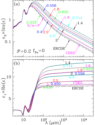
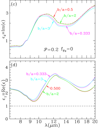
Figure 7: Same as Fig. 6 but for ${\cal P}=0.2$. Compared to the ${\cal P}=0$ case, $\epsilon_{2}$ is generally lower, and $\epsilon_{1}$ at long wavelengths is reduced.

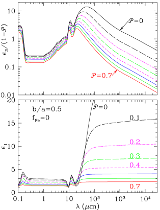
Figure 8: ${\rm Im}(\epsilon)$ and ${\rm Re}(\epsilon)$ for $b/a=0.5$, for various porosities ${\cal P}$.

Because astrodust grains must provide a substantial opacity at far-infrared wavelengths, $\epsilon_{2}$ must be relatively large in the far-infrared – for example, for ${\cal P}=0$ and $b/a=1.8$, we find $\epsilon_{2}(100\micron)\approx 20$, and low frequency dielectric constant $\epsilon_{1}(\omega\rightarrow 0)\approx 40$.

What values of $\epsilon$ are physically plausible? Consider some examples of strong dielectrics. Crystalline alumina (Al₂O₃) has $\epsilon_{1}(\omega\!\rightarrow\!0)=11.5$ along the crystal axis, magnetite (Fe₃O₄) has $\epsilon_{1}(\omega\!\rightarrow\!0)\approx 20$, and barium oxide (BaO) has $\epsilon_{1}(\omega\!\rightarrow\!0)\approx 34$ (Young & Frederikse 1973): large values do occur for some minerals. For ${\cal P}=0$ and $0.6\lesssim b/a<1.8$, the values found here for astrodust are outside this range; while not physically impossible, such models seem unrealistic.

Porosity, by increasing the grain volume, allows the required absorption to be provided by a more moderate dielectric function. Figure 7 shows $\epsilon$ if the porosity is taken to be ${\cal P}=0.2$. For $b/a=2$, we now find $\epsilon_{2}(100\micron)\approx 1$ and $\epsilon_{1}(\omega\rightarrow 0)\approx 8$. Figure 8 shows results for $b/a=0.5$ and porosities ${\cal P}$ from 0 to 0.7 .

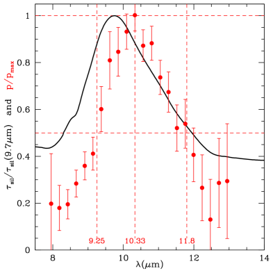
Figure 9: Points: Normalized polarization $p(\lambda)/p_{\rm max}$ toward WR48A and WR112=AFGL2014 (Wright et al. 2002). Curve: Extinction toward Cyg OB2-12 (Hensley & Draine 2020b).

6 Polarization Near the Silicate Resonances

6.1 Polarization Cross Section in the Electric Dipole Limit

By construction, the above dielectric functions all give the same $\lambda>1\micron$ opacity as a function of wavelength. However, they differ in polarization cross sections. The polarization cross section in the Rayleigh limit ($a\ll\lambda$) is:

$$C_{\rm pol}^{\rm(ed)}(\lambda) \equiv \frac{1}{4}\left[C_{\rm abs}^{\rm(ed)}({\bf E}\parallel\hat{\bf a}_{2})+C_{\rm abs}^{\rm(ed)}({\bf E}\parallel\hat{\bf a}_{3})\right]-\frac{1}{2}C_{\rm abs}^{\rm(ed)}({\bf E}\parallel\hat{\bf a}_{1})~{}~{}~{}{\rm for~{}ellipsoids,}$$ (17)

$$= \frac{1}{2}\left[C_{\rm abs}^{\rm(ed)}({\bf E}\perp\hat{\bf a})-C_{\rm abs}^{\rm(ed)}({\bf E}\parallel\hat{\bf a})\right]~{}~{}~{}{\rm for~{}oblate~{}spheroids,}$$ (18)

$$= \frac{1}{4}\left[C_{\rm abs}^{\rm(ed)}({\bf E}\parallel\hat{\bf a})-C_{\rm abs}^{\rm(ed)}({\bf E}\perp\hat{\bf a})\right]~{}~{}~{}{\rm for~{}prolate~{}spheroids,}$$ (19)

where we assume each grain to be spinning around the principal axis of largest moment of inertia $\hat{\bf a}_{1}$ (i.e., $\hat{\bf a}_{1}\parallel{\bf J}$, where ${\bf J}$ is the angular momentum). For spheroids with specified axis ratio $b/a$, we calculate $C_{\rm pol}$ using standard formulae (e.g., Bohren & Huffman 1983; Draine & Lee 1984). For the ERCDE and CDE2 shape distributions, we calculate $C_{\rm pol}^{\rm(ed)}(\lambda)$ using Eq. (31) and (33) from Draine & Hensley (2017). Each choice of grain shape and ${\cal P}$ leads to different predictions for $C_{\rm pol}^{\rm(ed)}(\lambda)$. By comparing the predicted $C_{\rm pol}^{\rm(ed)}(\lambda)$ to the observed polarization profile, we hope to narrow the domain of allowed values of ${\cal P}$ and grain shape.

Figure 9 shows the observed 8–13$\micron$ polarization profile in the ISM (Wright et al. 2002). There is a significant offset between the polarization profile (peaking near $\sim$$10.3\micron$) and the extinction profile (peaking near $9.75\micron$). Such an offset is theoretically expected, because $C_{\rm ran}^{\rm(ed)}(\lambda)$ and $C_{\rm pol}^{\rm(ed)}(\lambda)$ depend differently on $\epsilon(\lambda)$.

Figure 10 shows the theoretical $[C_{\rm pol}^{\rm(ed)}/(1-{\cal P})V]_{\rm Ad}$ from 7–40$\micron$, for spheroids with porosity ${\cal P}=0.2$, and various axis ratios $b/a$, as well as for the ERCDE and CDE2 shape distributions. By construction, these models have identical absorption profiles $C_{\rm ran}^{\rm(ed)}(\lambda)/(1-{\cal P})V_{\rm Ad}$. As expected, spheroids with more extreme axis ratios have larger $[C_{\rm pol}^{\rm(ed)}/V]_{\rm Ad}$. The CDE2 and ERCDE shape distributions have $[C_{\rm pol}^{\rm(ed)}(\lambda)/V]_{\rm Ad}$ that are similar to oblate spheroids with $b/a\approx 3$.

6.2 Grain Shape

In addition to affecting the overall magnitude of $C_{\rm pol}^{\rm(ed)}/V$, the grain shape also affects the shape of the polarization profile. Figures 10b and 10d show normalized polarization profiles. Varying the grain shape from oblate to prolate systematically shifts the $10\micron$ and $18\micron$ polarization profiles to longer wavelengths. Figure 10d shows that the short-wavelength side of the $10\micron$ profile shifts by $\sim$$0.19\micron$ as $b/a$ varies from 3 to $1/3$. Observations of the $10\micron$ polarization profile therefore provide a way to constrain the grain shape.

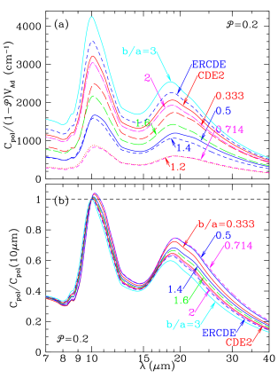
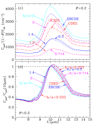
Figure 10: (a) $C_{\rm pol}^{\rm(ed)}/(1-{\cal P})V_{\rm Ad}$ and (b) normalized profile $C_{\rm pol}^{\rm(ed)}/C_{\rm pol}^{\rm(ed)}(10\micron)$ for spheroids with different axis ratios $b/a$, for the ERCDE distribution with $L_{\rm min}=0.05$, and for the CDE2 distribution, for dielectric functions that reproduce $C_{\rm abs}(\lambda)$ with ${\cal P}=0.2$. The polarization profile in (b) and (d) is seen to be sensitive to the assumed grain shape. Polarization for the CDE2 and ERCDE shape distributions is similar to oblate spheroids with $b/a\approx 3$.

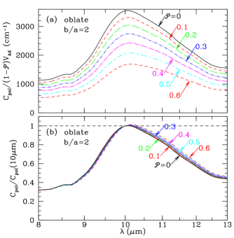
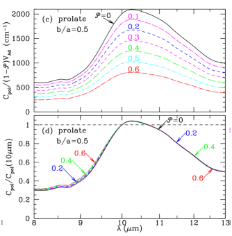
Figure 11: Polarization cross section in the 8–13$\micron$ region for $b/a=3$ (oblate) and $b/a=0.333$ (prolate) spheroids for selected porosity ${\cal P}$. The shape of the polarization profile depends only weakly on ${\cal P}$.

Figure 10b also shows that the strength of the 20$\micron$ polarization relative to the $10\micron$ polarization is sensitive to grain shape: the ratio $C_{\rm pol}(19\micron)/C_{\rm pol}(10\micron)$ changes from $0.57$ to $0.70$ as $b/a$ varies from 3 to $1/3$.

Lee & Draine (1985) argued that the polarized 10$\micron$ feature toward the BN object was best fit by oblate spheroids. However, their analysis was not self-consistent, because it adopted a single dielectric function that had been “derived” from the extinction assuming the grains to be spherical; this dielectric function was then used to calculate extinction vs. $\lambda$ for nonspherical grains. We now treat the problem self-consistently.

For each choice of grain shape and ${\cal P}$ we have a different dielectric function $\epsilon(\lambda;b/a,{\cal P})$, constrained to reproduce the observed absorption, but giving a distinct polarization profile. By comparing the models with spectropolarimetric observations, we hope to narrow the range of grain shapes consistent with observations. Figure 12 shows a goodness-of-fit metric

$$\chi^{2}\equiv\sum_{j=1}^{N_{\rm dat}}\frac{1}{\sigma_{j}^{2}}\left[\frac{p_{\rm obs}(\lambda_{j})}{p_{\rm max}}-A\frac{C_{\rm pol}^{\rm(ed)}(\lambda_{j})}{C_{\rm pol}^{\rm(ed)}(10\micron)}\right]^{2}~{}~{}~{},$$ (20)

for different axis ratios and selected ${\cal P}$, where the $N_{\rm dat}=22$ measurements $p_{\rm obs}(\lambda_{j})$ and uncertainties $\sigma_{j}$ (shown in Figure 9) are from Wright et al. (2002), and the scale factor $A$ is adjusted to minimize $\chi^{2}$ for each model. Figure 12 also shows $\chi^{2}$ for selected ${\cal P}$ for the CDE2 and ERCDE continuous distributions of ellipsoidal shapes.

We have 3 adjustable parameters: $b/a$, ${\cal P}$, and the factor $A$ in Eq. (20). We have no a priori constraint on axis ratio $b/a$, other than that it be large enough to be able to reproduce the observed polarization of starlight; allowed values of $b/a$ are delineated by Draine & Hensley (2020) for different ${\cal P}$. We have no a priori constraint on porosity, other than $0\leq{\cal P}<1$. If the measurement uncertainties $\sigma_{j}$ are independent and correctly estimated, we would expect to have a minimum $\chi^{2}\gtrsim 22-3=19$ (the dashed line in Figures 12a-d). Recognizing that the errors may have been under- or over-estimated, we are not concerned if the minimum of $\chi^{2}$ differs somewhat from 19.

It is evident from Figure 12 that oblate and prolate spheroids can both provide acceptable fits, depending on ${\cal P}$. The best fit is found for $a/b=3$ and ${\cal P}=0$.

We favor modest axis ratios, e.g., $a/b\approx 2$, or $b/a\approx 1.6$, for several reasons:

1. The distribution of grain sizes and shapes may be due in part to fragmentation. Fragmentation produces fragments with typical axis ratios $\sim 1\!:\!\sqrt{2}\!:\!2$, at least for larger (cm-sized) bodies (Fujiwara et al. 1978).

2. For extreme axis ratios, the observed polarization of starlight would require only a small fractional alignment of the $a\gtrsim 0.1\micron$ grains (see discussion in Draine & Hensley 2020). Although the physics of grain alignment remains uncertain, some analyses suggest that $a\gtrsim 0.15\micron$ grains will be rotating suprathermally (Purcell 1979; Draine & Weingartner 1996) and may be expected to have high alignment fractions. If so, the axis ratios should be more modest, perhaps $b/a\approx 1.4-1.8$, or $a/b\approx 1.6-2.5$.

3. The observed ratio of polarized submm emission to starlight polarization is sensitive to grain shape. For the present model (with both starlight extinction and FIR-submm emission dominated by a single grain type – astrodust) we favor modest axis ratios $b/a\approx 0.5$ (Draine & Hensley 2020; Hensley & Draine 2020a).

It should be kept in mind that $\chi^{2}$ in Fig. 12 is based on difficult observations of linear polarization (Fig. 9) made on only 2 stars.

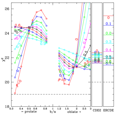
Figure 12: Figure-of-merit $\chi^{2}$ (see Eq. 20) for spheroids as a function of axis ratio $b/a$, for selected values of ${\cal P}$. The dashed line shows the expected value of $\chi^{2}\approx 19$ if the model were perfect, and errors are random and correctly estimated. The panels on the right show $\chi^{2}$ for the CDE2 and ERCDE shape distributions; with 2 degrees of freedom, we would expect $\chi^{2}=20$ (dashed line). The best fit is found for prolate spheroids with $a/b=3$ and ${\cal P}=0$.

6.3 Porosity

Figure 11 shows an expanded view of the 10$\micron$ polarization profile, for different values of ${\cal P}$. We see that for fixed shape $b/a=2$, varying ${\cal P}$ has less of an effect on the polarization profile than does varying the grain shape (compare Figures 10d and 11d).

Figure 12 shows $\chi^{2}$ vs. $b/a$ for spheroids with selected porosities ${\cal P}$, and $\chi^{2}$ for ellipsoids with the CDE2 or ERCDE shape distributions and different porosities. While the best fits to the observed polarization profiles are found for the more extreme prolate spheroids ($a/b=3$) and ${\cal P}=0$, the fits appear acceptable for all of the prolate cases, and for many of the oblate spheroids as well. Only strongly oblate shapes ($b/a>2$) with low porosities (${\cal P}<0.5$) are strongly disfavored. For the CDE2 and ERCDE shape distributions, the best fits are found for the highest porosities.

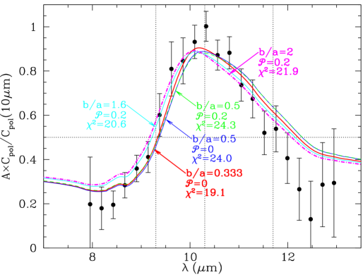
Figure 13: Data points: average polarization profile $p_{\rm obs}(\lambda)/p_{\rm max}$ measured for WR48A and WR112, two sightlines through the diffuse ISM (Wright et al. 2002). Curves: $A\times C_{\rm pol}/C_{\rm pol}(10\micron)$ for selected models, with the factor $A$ adjusted to minimize $\chi^{2}$ [see Eq. (20)]. The best fit shown (red) is for $b/a=0.333$ prolate spheroids with ${\cal P}=0$. Other examples of good fits are $b/a=0.5$ prolate spheroids with ${\cal P}=0$ and $0.2$, and $b/a=1.6$ and $2$ oblate spheroids with ${\cal P}=0.2$.

6.4 Polarization Profile: Examples

Figure 13 shows the polarization measured toward WR48A and WR112 (Wright et al. 2002) together with selected models that are in good agreement with the observations. The best-fitting model uses prolate spheroids with porosity ${\cal P}=0$, and axis ratio $a/b=3$, but fits that are almost as good are provided by $a/b=2$ and ${\cal P}=0$ or ${\cal P}=0.2$. Also shown are oblate models with $b/a=1.6$ and porosities ${\cal P}=0$ and $0.4$.

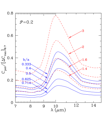
Figure 14: $C_{\rm pol}/[\Delta C_{\rm ran}]_{9.7\mu{\rm m}}$ for oblate (red) and prolate (blue) spheroids with varying axis ratio $b/a$, for porosity ${\cal P}=0.2$.

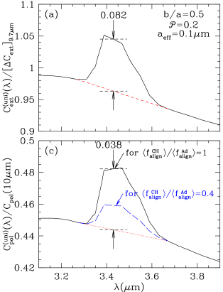
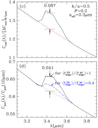
Figure 15: CH feature in extinction and polarization, calculated for prolate astrodust grains with $a/b=2$, porosity ${\cal P}=0$. (a) and (c): Extinction relative to extinction in the $9.7\micron$ silicate feature, for $a_{\rm eff}=0.1\micron$ and $0.3\micron$. For $a_{\rm eff}=0.3\micron$, scattering increases the extinction by $\sim$40%. (b) and (d): Polarization relative to polarization at $10\micron$, for $a_{\rm eff}=0.1\micron$ and $0.3\micron$. Solid black curve: assuming the CH absorber is uniformly mixed with the silicate material in astrodust. Dashed curve: estimated polarization for $\langle f_{\rm align}^{\rm CH}\rangle/\langle f_{\rm align}^{\rm Ad}\rangle=0.4$ (see text), which could correspond to the CH absorber being concentrated in a surface layer with thickness $\Delta\approx 0.01\micron$ (see Fig. 16).

7 Infrared and Submm Polarization

The objective of this section is to relate the polarization in the $10\micron$ feature to polarization at other wavelengths, as a model prediction. Of particular interest are (1) polarization in the far-infrared and submm thermal continuum, and (2) polarization in the $3.4\micron$ extinction feature produced by CH stretching modes in aliphatic hydrocarbons.

Consider a population of grains, each assumed to be spinning around its principal axis $\hat{\bf a}_{1}$. Let $a$ be the spherical-volume-equivalent grain radius. The fractional alignment of grains of size $a$ with the local magnetic field ${\bf B}_{0}$ is

$$f_{\rm align}(a)\equiv\frac{3}{2}\left[\langle(\hat{\bf a}_{1}\cdot\hat{\bf B}_{0})^{2}\rangle-\frac{1}{3}\right]~{}~{}~{},$$ (21)

with $f_{\rm align}=0$ for random orientations, and $f_{\rm align}=1$ for perfect alignment of $\hat{\bf a}_{1}$ with ${\bf B}_{0}$. The mass-weighted alignment of the astrodust material is

$$\langle f_{\rm align}^{\rm Ad}\rangle\equiv\frac{\int_{a_{\rm min}}^{a_{\rm max}}daf_{\rm align}(a)a^{3}(dn/da)}{\int_{a_{\rm min}}^{a_{\rm max}}da\,a^{3}(dn/da)}~{},$$ (22)

where $n(a)$ is the number of grains smaller than $a$.

Let $\gamma$ be the angle between the magnetic field ${\bf B}_{0}$ and the line of sight $\hat{\bf z}$. Let $\hat{\bf x}$ and $\hat{\bf y}$ be $\perp$ and $\parallel$ to the projection of ${\bf B}_{0}$ on the plane of the sky, and let $\tau_{x}$, $\tau_{y}$ be the optical depths for ${\bf E}\parallel\hat{\bf x}$, ${\bf E}\parallel\hat{\bf y}$. Provided the grains are in the Rayleigh limit, with $C_{\rm pol}\propto V$, the fractional polarization $p$ per unit $10\micron$ feature depth $\Delta\tau_{9.7\mu{\rm m}}$ is just

$$\frac{p_{\rm ext}(\lambda)}{\Delta\tau_{9.7\mu{\rm m}}}=\frac{1}{\Delta\tau_{9.7\mu{\rm m}}}\left[\frac{e^{-\tau_{y}}-e^{-\tau_{x}}}{e^{-\tau_{x}}+e^{-\tau_{y}}}\right]\approx\frac{\tau_{x}-\tau_{y}}{2\Delta\tau_{9.7\mu{\rm m}}}\approx\frac{C_{\rm pol}(\lambda)}{[\Delta C_{\rm ran}]_{9.7\mu{\rm m}}}\langle f_{\rm align}^{\rm Ad}\rangle\sin^{2}\gamma~{}~{}~{}.$$ (23)

The polarizing ability of astrodust grains, relative to extinction in the 9.7$\micron$ feature, is shown in Figure 14 for ${\cal P}=0.2$ and selected shapes. For $b/a=0.5$ and ${\cal P}=0.2$ we have

$$\frac{C_{\rm pol}^{\rm(ed)}(10\micron)}{[\Delta C_{\rm ran}^{\rm(ed)}]_{9.7\mu{\rm m}}}\approx 0.29~{}.$$ (24)

7.1 3.4$\mu$m Feature Polarization

CH absorption will produce a polarization feature at $3.4\micron$. We define an effective alignment fraction for the CH:

$$\langle f_{\rm align}^{\rm CH}\rangle\equiv\frac{\int daf_{\rm align}(a)f_{\rm CH}(a)a^{3}(dn/da)}{\int daf_{\rm CH}(a)a^{3}(dn/da)}$$ (25)

where $f_{\rm CH}(a)$ is the fraction of the volume of grains of radius $a$ occupied by the $3.4\micron$ absorber. If the CH absorber is uniformly distributed through the astrodust, then $f_{\rm CH}(a)$ is independent of $a$, and $\langle f_{\rm align}^{\rm CH}\rangle=\langle f_{\rm align}^{\rm Ad}\rangle$.

At 3.4$\micron$, $a\gtrsim 0.1\micron$ grains are large enough that scattering begins to be important, and the extinction and polarization cross sections no longer vary linearly with grain mass. Let $C_{\rm ext}^{\rm(uni)}(\lambda)$ and polarization $C_{\rm pol}^{\rm(uni)}(\lambda)$ (see Figure 15) be extinction and polarization cross sections calculated for the case of uniformly-distributed CH absorption (i.e., $f_{\rm CH}$ independent of $a$).

For $0.1<a<0.3\micron$ grains, the 3.4$\micron$ feature would have polarization, relative to $10\micron$ polarization,

$$\frac{[\Delta p]_{3.4\mu{\rm m}}}{p(10\micron)}=\frac{\Delta C_{\rm pol}^{\rm(uni)}(3.41\micron)}{C_{\rm pol}(10\micron)}\frac{\langle f_{\rm align}^{\rm CH}\rangle}{\langle f_{\rm align}^{\rm Ad}\rangle}\approx 0.040\frac{\langle f_{\rm align}^{\rm CH}\rangle}{\langle f_{\rm align}^{\rm Ad}\rangle}~{},$$ (26)

where the value $0.040$ is intermediate between $0.038$ for $a_{\rm eff}=0.1\micron$ and $0.041$ for $0.3\micron$ (see Figures 15c,d). The Quintuplet sources near the Galactic Center have (Chiar et al. 2006)

$$\frac{[\Delta p]_{3.4\micron}}{p(10\micron)} = \frac{(0.0006\pm 0.0013)}{(0.090\pm 0.003)}\approx 0.007\pm 0.015~{}~{}~{}{\rm for~{}GCS3-II}$$ (27)

$$= \frac{(0.0015\pm 0031)}{(0.102\pm 0.015)}~{}~{}~{}\approx 0.015\pm 0.030~{}~{}~{}{\rm for~{}GCS3-IV}~{};$$ (28)

the error bars are claimed to be 99% confidence intervals. If the CH and the silicate are in the same aligned grains, with $\langle f_{\rm align}^{\rm CH}\rangle/\langle f_{\rm align}^{\rm Ad}\rangle=1$, the predicted value (26) exceeds the observed values by a factor $\sim$3. Therefore, the CH absorber and the silicate absorber cannot be identically distributed. How can the astrodust hypothesis accomodate this?

We are postulating that astrodust contains both silicate and carbonaceous material, in approximately constant ratios. However, it may be that only a fraction of the carbonaceous material produces $3.4\micron$ absorption. Mennella et al. (1999, 2002) argue that the $3.4\micron$ CH absorption feature is the result of exposure of carbonaceous material to H atoms. If so, the CH absorption may be concentrated in “activated” surface layers on the grains, where hydrogenation by inward-diffusing H atoms has produced the CH bonds responsible for the absorption feature.

The observed wavelength-dependence of starlight polarization requires that grains smaller than $\sim$$0.1\micron$ be minimally aligned (Kim & Martin 1995; Draine & Fraisse 2009). For grain size distributions consistent with the observed interstellar reddening, most of the grain surface area is provided by small grains.

Previous studies have considered the possibility that the $3.4\micron$ absorption arises in hydrocarbon mantles with silicate cores, concluding that the 3.4$\micron$ polarization, relative to silicate feature polarization, is fairly insensitive to whether the 3.4$\micron$ absorber is in a mantle or mixed through the grain (Li & Greenberg 2002; Li et al. 2014). This is true for grains for which the ratio of $3.4\micron$ absorption to silicate absorption is constant. However, if the $3.4\micron$ absorption were concentrated in a thin surface layer with thickness independent of grain size, then small grains would make a greater contribution to $3.4\micron$ absorption (relative to silicate absorption) than would larger grains. Since small grains are relatively unaligned, and account for most of the total grain surface area, the $3.4\micron$ absorption would be skewed toward the unaligned grain population, resulting in smaller values of $[\Delta p]_{3.4\micron}/p(10\micron)$ than would otherwise be expected.

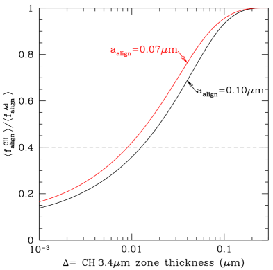
Figure 16: Fractional alignment of CH $3.4\micron$ absorbers relative to fractional alignment of the silicate absorbers as a function of the thickness $\Delta$ of the CH $3.4\micron$ absorption layer (see text). Upper limits on CH $3.4\micron$ polarization appear to require $\langle f_{\rm align}^{\rm CH}\rangle/\langle f_{\rm align}^{\rm Ad}\rangle\lesssim 0.4$, or $\Delta\lesssim 0.01\micron$ if the IR opacity is dominated by a single grain type.

If the CH $3.4\micron$ absorber is in a surface layer of thickness $\Delta$, then the aligned fraction for CH $3.4\micron$ absorbers is

$$\langle f_{\rm align}^{\rm CH}\rangle\approx\frac{\int daf_{\rm align}(a)\left[a^{3}-({\rm max}(a-\Delta,0))^{3}\right](dn/da)}{\int da\left[a^{3}-({\rm max}(a-\Delta,0))^{3}\right](dn/da)}~{}~{}.$$ (29)

Figure 16 shows the ratio $\langle f_{\rm align}^{\rm CH}\rangle/\langle f_{\rm align}^{\rm Ad}\rangle$ for a MRN size distribution ($dn/da\propto a^{-3.5}$, $0.001\micron<a<0.30\micron$) and a step-function alignment fraction ($f_{\rm align}=0$ for $a<a_{\rm align}$, $f_{\rm align}=const$ for $a>a_{\rm align}$). If $a_{\rm align}\approx 0.1\micron$ and $\Delta=0.01\micron$, the polarization in the CH $3.4\micron$ feature would be suppressed by a factor $\sim$0.4 relative to the value if the CH $3.4\micron$ absorbers were uniformly distributed in the astrodust material, and astrodust would have

$$\frac{[\Delta p]_{3.4\mu{\rm m}}}{p(10\micron)}\approx 0.040\times 0.4\approx 0.016~{}~{}.$$ (30)

This predicted $3.4\micron$ polarization relative to 10$\micron$ polarization is marginally consistent with Eqs. (27,28), currently the best upper limits on $[\Delta p]_{3.4}/p(10\micron)$.

Further improvements in mid-IR spectropolarimetry should be able to detect the predicted polarization (30) associated with the $3.4\micron$ feature if it originates near the surfaces of astrodust grains. If the silicate and carbonaceous material are distributed in the same grains, as in our astrodust model, this would allow determination of the thickness $\Delta$ of the CH “activated” surface layers.

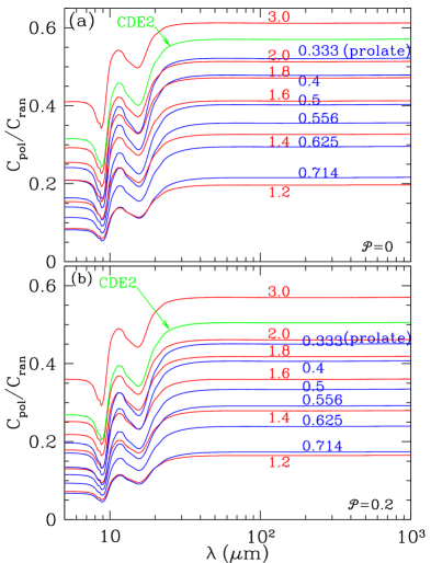
Figure 17: (a) $C_{\rm pol}/C_{\rm ran}$ for oblate (red) and prolate (blue) spheroids with varying axis ratio $b/a$, for dielectric functions with porosity ${\cal P}=0$ and $f_{\rm Fe}=0$. (b) Same as (a), but for ${\cal P}=0.2$. For modest axis ratios (e.g., $0.5\lesssim b/a\lesssim 1.6$), changing the porosity from ${\cal P}=0$ to $0.2$ reduces $C_{\rm pol}/C_{\rm ran}$ by $\sim$$20\%$.

7.2 Far-Infrared and Submm Polarization

Optically-thin thermal emission from astrodust grains has polarization fraction (Draine & Hensley 2017)

$$p_{{\rm em},\lambda}^{\rm Ad} = \left[\frac{C_{x}-C_{y}}{C_{x}+C_{y}}\right]_{\lambda}^{\rm Ad}=\left[\frac{C_{\rm pol}}{C_{\rm ran}}\right]_{\lambda}^{\rm Ad}\times\frac{\langle f_{\rm align}^{\rm Ad}\rangle\sin^{2}\gamma}{1-\left[C_{\rm pol}/C_{\rm ran}\right]_{\lambda}^{\rm Ad}\langle f_{\rm align}^{\rm Ad}\rangle\left(\sin^{2}\gamma-\frac{2}{3}\right)}$$ (31)

$$\approx \left[\frac{C_{\rm pol}}{C_{\rm ran}}\right]_{\lambda}^{\rm Ad}\times\langle f_{\rm align}^{\rm Ad}\rangle\sin^{2}\gamma~{}~{}~{}.$$ (32)

At long wavelengths ($\lambda>50\micron$), the large values of $\epsilon_{1}$ (see Figs. 6, 7) result in relatively large values of $[C_{\rm pol}/C_{\rm ran}]_{\lambda}^{\rm Ad}$. Fig. 17 shows $[C_{\rm pol}/C_{\rm ran}]_{\lambda}^{\rm Ad}$ from $\lambda=5\micron$ out to $1\,{\rm mm}$ for different values of $b/a$, for ${\cal P}=0$ and $0.2$. We have seen above that the silicate polarization profile can be fit well by prolate spheroids with $b/a\lesssim 0.5$. For $b/a=0.5$, Fig. 17 shows that such silicate-bearing grains have $[C_{\rm pol}/C_{\rm ran}]_{\lambda}^{\rm Ad}\approx 0.30$ at submm wavelengths (for ${\cal P}=0.2$).

Planck has measured the polarization of the $850\micron$ emission from the diffuse ISM. The highest fractional polarization observed (the 99.9th percentile) is estimated to be $0.220_{-.014}^{+0.035}$ (Planck Collaboration et al. 2018). For optimal viewing geometry ($\sin^{2}\gamma=1$). such high polarizations could be produced by $b/a=0.5$ prolate spheroids with high degrees of alignment ($\langle f_{\rm align}^{\rm Ad}\rangle\approx 0.7$).

8 Discussion

8.1 Shape of the Silicate-Bearing Grains

When this study was initiated, it was hoped that the shape of the silicate polarization profile would strongly favor certain grain shapes and porosities. However, we find that, for self-consistent dielectric functions, the shape of the polarization profile depends only weakly on shape and porosity. Existing observations of only the extinction and polarization of the 10$\micron$ silicate feature appear to allow both prolate and oblate shapes. According to Figure 12, the best-fitting shape for ${\cal P}=0$ is an extreme prolate shape, $b/a=3$, but we find that oblate shapes with $b/a\approx 1.4$ or $1.6$ provide fits that are almost as good. Other polarization data – the strength of starlight polarization at optical wavelengths, and of polarized thermal emission at submm wavelengths – provide additional constraints on grain shape and porosity.

The CDE2 and ERCDE shape distributions also give $10\micron$ polarization profiles that are in good agreement with the observed profile. However, these shape distributions are not practical for modeling interstellar grains, because to model the polarization of starlight we require extinction cross sections at wavelengths comparable to the grain size. Such calculations for ellipsoids are time-consuming, and even for a single grain mass and wavelength one would need to sample many different ellipsoidal shapes in order to represent a continuous distribution of ellipsoidal shapes such as CDE2 or ERCDE.

8.2 Porosity

As seen above (Fig. 12), the porosity is only minimally constrained by the shape of the $10\micron$ polarization profile. Draine & Hensley (2020) show that the strongest constraint on porosity is from the strength of the polarization (both polarization of starlight, and polarization of submm emission), which limit the porosity to a maximum value that depends on grain shape. Extreme porosities are ruled out.

8.3 The Silicate Absorption Profile

The present investigation was based upon the best available observational determinations of the absorption by interstellar dust over a wavelength range covering the 9.7$\micron$ and $18\micron$ silicate features. The best data are from the Spitzer IRS instrument, observing Cyg OB2-12 (Ardila et al. 2010; Fogerty et al. 2016; Hensley & Draine 2020b). A weak broad absorption feature at $11.1\pm 0.10\micron$ is seen in the spectra of a number of heavily obscured objects (Wright et al. 2016; Duy et al. 2020), which is interpreted as an Mg-rich olivine, possibly the end-member forsterite Mg₂SiO₄. Our determination of the silicate profile toward Cyg OB2-12 does not include any obvious feature near $11.1\micron$, but this may be the result of uncertainties in estimation of the underlying emission from Cyg OB2-12.

With the termination of the cold Spitzer mission, spectrophotometry in this wavelength range must be done through the 8–14$\micron$ atmospheric window until the advent of the Mid Infrared Instrument (MIRI) on the James Webb Space Telescope (JWST), which should provide $\lambda/\Delta\lambda=5000$ spectroscopy over the 5–28$\micron$ range.

Spectrophotometry with MIRI is expected to significantly improve our knowledge of the silicate absorption in the 5–28$\micron$ range. If spectrophotometry with MIRI confirms the “wiggles” in the Spitzer IRS spectra and shows them to be due to the interstellar extinction (rather than the stellar atmospheres), these features will provide clues to the composition and structure of the interstellar amorphous silicate material, which laboratory synthesis could attempt to replicate.

8.4 Polarization in the Silicate Features

For grain shapes ($a/b\approx 0.5$) and likely degree of alignment ($\langle f_{\rm align}^{\rm Ad}\rangle\approx 0.7$) that appear to be consistent with (1) the silicate polarization profile (2) the optical-UV polarization of starlight, and (3) typical levels of submm polarization observed by Planck, we expect the silicate feature, observed in extinction, to produce polarization. For $b/a=0.5$ and ${\cal P}=0.2$ we have

$$\frac{p(10\micron)}{\Delta\tau_{9.7}}\approx 0.29\langle f_{\rm align}^{\rm Ad}\rangle\sin^{2}\gamma$$ (33)

[see eq. (23,24)]. If $\langle f_{\rm align}^{\rm Ad}\rangle\approx 0.7$, we would expect to find values of $p(10\micron)/\Delta\tau_{9.7}$ as large as $\sim 0.20$ for the most favorable geometries ($\sin^{2}\gamma\rightarrow 1$).

Smith et al. (2000) present the results of 10$\micron$ spectroscopy and polarimetry of 55 infrared sources. In their sample, the highest observed values of $p(10\micron)/\Delta\tau_{9.7\mu{\rm m}}$ are $0.038$ (the BN object in OMC1) and $0.035$ (Galactic Center source GCS IV at $(\ell,b)=(0.16^{\circ},-0.06^{\circ})$). Why have higher values of $p(10\micron)/\Delta\tau_{9.7}$ not been seen?

Most of the 55 sources in the Smith et al. (2000) atlas are infrared sources embedded in star-forming molecular clouds (e.g., the BN object) – for which our diffuse ISM-based estimates of $b/a$ and $\langle f_{\rm align}^{\rm Ad}\rangle$ may not apply. The polarizing efficiency of grains in dark clouds is observed to be reduced (Whittet et al. 2008). The grain alignment in dark clouds may not achieve values of $\langle f_{\rm align}^{\rm Ad}\rangle$ as high as observed in the diffuse ISM; in addition, the grain shapes within these clouds might conceivably be less elongated than in the diffuse ISM. Furthermore, the magnetic fields in these turbulent clouds may have an appreciable disordered component, which would lower the degree of polarization.

The Galactic Center source GCS IV is located in an area of the sky where Planck found a relatively low fractional polarization at $850\micron$ (Planck Collaboration et al. 2015a) – the $850\micron$ polarization appears to be only $\sim$$2\%$, small compared to the highest values ($\gtrsim$20%: Planck Collaboration et al. 2018) observed by Planck, presumably indicating some combination of low degrees of alignment and disordered and/or unfavorable magnetic field geometry in the dust-containing regions (i.e., low effective values of $\langle f_{\rm align}^{\rm Ad}\rangle\sin^{2}\gamma$). Given the low fractional ($\sim$$2\%$) polarization of the diffuse 850$\micron$ emission in this field, we would expect a relatively low value of $p(10\micron)/\Delta\tau_{9.7}$ on the sightline to GCS IV, as observed.

It would be of great value to have measurements of $p(10\micron)/\Delta\tau_{9.7}$ in regions where Planck finds high values of $p(850\micron)$, ideally using sources where the bulk of the extinction arises from the diffuse ISM (rather than being local to the source). For Cyg OB2-12 we predict $p(10\micron)\approx(2.2\pm 0.3)$% (Draine & Hensley 2020), which should be measurable.

This paper has stressed the value of mid-infrared spectropolarimetry to constrain grain geometry and the dielectric function of the silicate material. The atlas of polarized spectra published by Smith et al. (2000) remains the “state-of-the-art”, but it is sobering to note in 2020 that all of the observations reported in that paper were taken prior to February 1993. It is regrettable that polarimetric capabilites were not included in either the Spitzer or JWST instrument suites, and disappointing that most large telescopes that have come into operation over the past three decades have not been equipped with IR spectropolarimetric instruments. The silicate polarization profile does depend on grain shape, but the best available spectropolarimetry (toward WR-48a and WR-112=AFGL2104) has estimated observational uncertainties that permit both oblate and prolate shapes. Spectropolarimetry with factor of $\sim 2$ higher signal/noise could remove this ambiguity, and reject the prolate or oblate shapes (or perhaps both!). The Canaricam instrument on the Gran Telescopio Canarias (Packham et al. 2005) appears to be the most capable instrument currently available for mid-infrared spectropolarimetry, and this instrument may be able to provide improved measurements of the wavelength-dependence of the silicate polarization.

It would also be of great value to have spectropolarimety extending shortward and longward of the atmospheric windows. Given the absence of polarimetry on JWST, a mid-IR spectropolarimeter on a high altitude balloon or on SOFIA (Packham et al. 2008) could provide valuable and unique constraints on models for the silicate-bearing interstellar grain population.

9 Summary

The principal findings of this study are as follows:

1. Observations of the far-infrared polarization fraction from $250\micron$ to $3\,{\rm mm}$ favor a model for interstellar dust where the opacity is dominated by a single grain material, which we term “astrodust.”

2. We use the observed 5–35$\micron$ extinction toward Cyg OB2-12 (Hensley & Draine 2020b), the opacity inferred from the observed far-infrared and submm emission (Hensley & Draine 2020c), plus other constraints (including depletion-based estimates of grain mass and volume), to derive the effective dielectric function $\epsilon(\lambda)$ for astrodust in the diffuse ISM. Astrodust material is $\sim$50% amorphous silicate, but also incorporates $\sim$$25\%$ of the carbon in diffuse clouds (an additional $\sim$$12\%$ of the carbon is in a population of PAH nanoparticles). The hydrocarbon material in the astrodust grains is assumed to be responsible for the $3.4\micron$ absorption feature in the diffuse ISM. The PAHs are assumed to be randomly-oriented; all of the polarized extinction and emission from the diffuse ISM is attributed to the astrodust grains.

   The derived $\epsilon(\lambda)$ depends on assumptions including the shape and porosity of the astrodust grains. The “astrodust” dielectric functions obtained here will be made available in computer-readable form at the time of publication.

3. For different grain shape and ${\cal P}$, we calculate the polarization cross section, and predict the wavelength dependence of polarization from the near-IR (3.4$\micron$) to mm wavelengths.

4. Comparing the predicted $C_{\rm pol}(\lambda)/V$ with the $8$–$13\micron$ polarization observed toward two WR stars (Wright et al. 2002), we conclude that:

   • The silicate-bearing grains can be approximated by either oblate or prolate spheroids: the existing polarimetric data do not definitively discriminate between oblate or prolate shapes.

   • With existing spectropolarimetry, the shape of the polarization profile is consistent with a wide range of porosities. Limits on porosity must come from considerations of the strength of the polarization, both the starlight polarization and the degree of polarization of the submm emission (Draine & Hensley 2020).

   • Future spectropolarimetry with improved signal/noise ratio has the potential to narrow the range of allowed shapes and porosities.

5. CH absorption in the aligned astrodust grains will produce a polarized extinction feature at 3.4$\micron$ [see Eq. (26)]:

   $$\frac{[\Delta p]_{3.4\mu{\rm m}}}{p(10\micron)}\approx 0.040\times\frac{\langle f_{\rm align}^{\rm CH}\rangle}{\langle f_{\rm align}^{\rm Ad}\rangle}~{}~{},$$ (34)

   where $\langle f_{\rm align}^{\rm Ad}\rangle$ is the mass-averaged alignment of the astrodust grains, and $\langle f_{\rm align}^{\rm CH}\rangle$ is the 3.4$\micron$ absorption feature-weighted fractional alignment. If the $3.4\micron$ absorbers are preferentially located near the grain surfaces, then the fact that small grains are minimally aligned implies $\langle f_{\rm align}^{\rm CH}\rangle/\langle f_{\rm align}^{\rm Ad}\rangle<1$, with the actual ratio dependent on the degree to which the $3.4\micron$ absorption is concentrated near grain surfaces. For $\langle f_{\rm align}^{\rm CH}\rangle/\langle f_{\rm align}^{\rm Ad}\rangle\lesssim 0.4$, the predicted $3.4\micron$ feature polarization is consistent with the observed upper limits on $3.4\micron$ feature polarization (Chiar et al. 2006). Such values would be consistent with the $3.4\micron$ absorption arising in surface zones of thickness $\Delta\lesssim 0.01\micron$. More sensitive 3.4$\micron$ polarimetry should be able to detect the predicted polarization in the 3.4$\micron$ feature.

Appendix A Magnetic Dipole Absorption by Metallic Fe inclusions

We assume that silicate-bearing grains contain ferromagnetic metallic Fe inclusions, randomly-distributed throughout the volume, with volume filling factor [see Eq. (7)]

$$f_{\rm fill}\approx\left(1-{\cal P}\right)\frac{0.12f_{\rm Fe}}{1-0.22f_{\rm Fe}}~{}~{}~{}.$$ (A1)

where $f_{\rm Fe}$ is the fraction of the iron in metallic inclusions. For a spheroidal grain with principal axes $\hat{\bf a}_{j}$, the magnetic-dipole contribution to the absorption is, for ${\bf H}\parallel\hat{\bf a}_{j}$,

$$C_{{\rm abs},j}^{\rm mag}=\frac{\omega V}{c}{\rm Im}\left[\frac{\mu_{\rm eff}-1}{1+L_{j}(\mu_{\rm eff}-1)}\right]~{},$$ (A2)

where $\mu_{\rm eff}$, the effective-medium estimate for the magnetic permeability of the grain material, is given by

$$\mu_{\rm eff}=1+4\pi\frac{f_{\rm fill}(\chi_{+}+\chi_{-})/3}{1-D_{b}f_{\rm fill}(\chi_{+}+\chi_{-})/3}~{},$$ (A3)

where

$$\chi_{\pm}=\frac{\omega_{\rm M}}{\omega_{0}-i\alpha_{G}\omega\mp\omega}~{},$$ (A4)

(Draine & Hensley 2013). $D_{b}$ in Eq. (A3) is the demagnetization factor perpendicular to the long axis of a prolate inclusion; for 2:1 prolate inclusions, $D_{b}=5.193$. $\alpha_{G}\approx 0.2$ is the Gilbert damping parameter, and $\omega_{\rm M}/2\pi=4.91\,{\rm GHz}$ for Fe (Draine & Hensley 2013). The parameter $\omega_{0}$ depends on the shape of the ferromagnetic inclusions, varying from $\omega_{0}/2\pi=1.53\,{\rm GHz}$ for spherical inclusions, to $\omega_{0}/2\pi=16.3\,{\rm GHz}$ for 2:1 prolate inclusions (see Table 2 of Draine & Hensley 2013).

Appendix B Dielectric Function for Astrodust Material from Optical to X-ray Wavelengths

We seek a provisional dielectric function $\epsilon_{\rm mat}^{\rm ox}(\lambda)$ for astrodust material at wavelengths $\lambda<\lambda_{0}\equiv 1\micron$ ($\hbar\omega>\hbar\omega_{0}\equiv 1.24\,{\rm eV}$). Let $\epsilon^{\rm ox}(\lambda)$ be the dielectric function for solid astrodust material with no voids and no Fe inclusions. We proceed as follows:

1. Because we expect the silicate-bearing grains to account for most of the far-infrared emission, these grains should be absorptive at the energies $0.5\lesssim 5\,{\rm eV}$ where the interstellar starlight energy density $u_{\nu}$ peaks [the Mathis et al. (1983) estimate for the radiation field has $\nu u_{\nu}$ peaking at $h\nu=1.32\,{\rm eV}$]. We assume

   $${\rm Im}(\epsilon_{\rm mat}^{\rm ox})\approx 0.20.~{}~{}~{}{\rm for}~{}~{}1\lesssim E\lesssim 5\,{\rm eV}~{}.$$ (B1)

   This is about twice as large as was assumed for astrosilicate by Draine & Lee (1984); Li & Draine (2001); Draine (2003); Draine & Li (2007). Adoption of a larger value of ${\rm Im}(\epsilon)$ at optical wavelengths is motivated by the finding (Planck Collaboration et al. 2016) that the far-infrared power per unit starlight extinction is about twice as large as had been estimated for the Draine & Li (2007) dust model and the MMP83 estimate for the starlight intensity.

2. For computational convenience in obtaining ${\rm Re}(\epsilon_{\rm mat}^{\rm ox})$ using the Kramers-Kronig relations, we extend $\epsilon_{\rm mat}^{\rm ox}$ into the IR:

   $${\rm Im}(\epsilon_{\rm mat}^{\rm ox})=0.20(1\micron/\lambda)^{2}~{}~{}~{}{\rm for}~{}\lambda>1\micron~{}.$$ (B2)

   The assumed form of Eq. (B2) for $\lambda>1\micron$ does not affect our final result, as we subsequently use $\epsilon_{\rm mat}^{\rm ir}$ to add to (or subtract from) $\epsilon_{\rm mat}^{\rm ox}$ at $\lambda>1\micron$ to comply with observational constraints [see Eq. (13)].

   

   

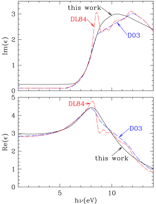
   Figure 18: Solid curves: real and imaginary part of $\epsilon$ for astrodust with ${{\cal P}}=0$. Dashed curves (D03): silicate dielectric function from Draine (2003). X-ray absorption edges are seen at 528 eV(O K), 700 eV(Fe L), … Dot-dashed curves (DL84): astrosilicate dielectric function from Draine & Lee (1984).

3. For $h\nu\gtrsim 8\,{\rm eV}$, we adopt a dielectric function similar to the “astrosilicate” dielectric function of (Draine & Lee 1984; Draine 2003), with a rapid increase in absorption when the photon energy is large enough to excite valence-band electrons to the (empty) conduction band.

4. Let $\alpha_{\rm mat}$ be the attenuation coefficient for radiation propagating through the matrix material. The attenuation coefficient is directly related to the imaginary part of the refractive index $m$:

   $$\alpha_{\rm mat}=\frac{4\pi}{\lambda}{\rm Im}(m)~{}~{}~{},$$ (B3)

   where $\lambda$ is the wavelength in vacuo. Because ${\rm Im}(\epsilon)={\rm Im}(m^{2})=2{\rm Re}(m){\rm Im}(m)$, we have

   $${\rm Im}(\epsilon_{\rm mat}^{\rm ox})=\frac{\lambda}{2\pi}{\rm Re}(m)\alpha_{\rm mat}~{}~{}~{}.$$ (B4)

   At high energies we expect ${\rm Re}(m)\approx 1$, and the absorption per atom is expected to be well-approximated by the mean photoelectric absorption cross sections $\sigma_{{\rm pe},j}$ of isolated atoms of element $j$,

   $$\alpha_{\rm mat}^{\rm ox}\approx\sum_{j}n_{j}\sigma_{{\rm pe},j}(h\nu)~{}~{}~{},$$ (B5)

   where $n_{j}$ is the number density of atoms $j$. Therefore, at high energies ($E>22\,{\rm eV}$) we take

   $${\rm Im}(\epsilon_{\rm mat}^{\rm ox})\approx\frac{\lambda}{2\pi}\sum_{j}n_{j}\sigma_{{\rm pe},j}~{}.$$ (B6)

   We approximate the photoelectric absorption cross sections $\sigma_{{\rm pe},j}(h\nu)$ by the photoionization fitting functions estimated for inner shell electrons by Verner & Yakovlev (1995) and for outer-shell electrons by Verner et al. (1996), implemented in the fortran code phfit2.f written by D.A. Verner.

   For $15<E<22\,{\rm eV}$, we adopt ${\rm Im}(\epsilon^{\rm ox})$ that connects our adopted $E<15\,{\rm eV}$ absorption (see Figure 18) to the absorption (B5) for $E>22\,{\rm eV}$.

5. The real part of the dielectric function is obtained using the Kramers-Kronig relations:

   $${\rm Re}\left(\epsilon_{\rm mat}^{\rm ox}(\omega)\right)=1+\frac{2}{\pi}\int_{0}^{\infty}\frac{{\rm Im}\left(\epsilon_{\rm mat}^{\rm ox}(x)\right)}{x^{2}-\omega^{2}}~{}xdx~{}.$$ (B7)

6. For nonzero porosity ${\cal P}$ and/or material with metallic Fe inclusions, we apply Bruggeman effective medium theory, and take the effective dielectric function $\epsilon_{\rm eff}$ to satisfy

   $$0=(1-{\cal P}-f_{\rm sv,Fe})\left(\frac{\epsilon_{\rm mat}-\epsilon_{\rm eff}}{\epsilon_{\rm mat}+2\epsilon_{\rm eff}}\right)+{\cal P}\left(\frac{1-\epsilon_{\rm eff}}{1+2\epsilon_{\rm eff}}\right)+f_{\rm sv,Fe}\left(\frac{\epsilon_{\rm Fe}-\epsilon_{\rm eff}}{\epsilon_{\rm Fe}+2\epsilon_{\rm eff}}\right)~{},~{}~{}~{}$$ (B8)

   where $f_{\rm sv,Fe}$ is the fraction of the solid volume contribued by Fe inclusions [see Eq. (7)]. The Fe inclusions and vacuum pores are both taken to be spherical (Bohren & Huffman 1983).

7. By construction, $\epsilon^{\rm ox}(\lambda)$ satisfies the Kramers-Kronig relations. In addition, we verify that our final $\epsilon$ satisfies the “f-sum rules” (Altarelli et al. 1972)

   $$\frac{m_{e}}{2\pi^{2}e^{2}}\int_{0}^{\infty}\omega{\rm Im}(\epsilon)d\omega=\sum_{j}n_{j}$$ (B9)

   $$\frac{m_{e}}{\pi^{2}e^{2}}\int_{0}^{\infty}\omega{\rm Im}(\sqrt{\epsilon})d\omega=\sum_{j}n_{j}~{}~{}~{},$$ (B10)

   where $n_{j}$ is the number density of electrons in atomic shell $j$. Figure 19 shows

   $$n_{\rm eff}(E)\equiv\frac{m_{e}}{2\pi^{2}e^{2}}\int_{0}^{E/\hbar}\omega{\rm Im}(\epsilon)d\omega$$ (B11)

   and

   $$n_{\rm eff}(E)\equiv\frac{m_{e}}{\pi^{2}e^{2}}\int_{0}^{E/\hbar}\omega{\rm Im}(\sqrt{\epsilon})d\omega~{}~{}~{}.$$ (B12)

Figure 19: $n_{\rm eff}(E)$ evaluated using Eq. (B11) and (B12) using the astrodust dielectric function for ${\cal P}=0$. The expected asymptotic limit $n_{\rm eff}=1.03\times 10^{24}\,{\rm cm}^{-3}$ for the $F_{\star}=0.5$ composition in Table 2 is shown as a dashed line.

Appendix C Dielectric Function for Grains with Ferromagnetic Inclusions

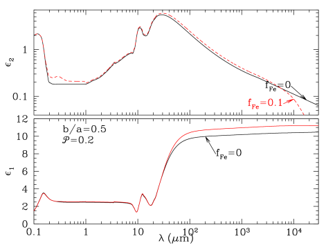
Figure 20: Dielectric function $\epsilon$ for $b/a=0.5$ prolate spheroids, for ${\cal P}=0.2$, and $f_{\rm Fe}=0$ and $0.1$, where $f_{\rm Fe}$ is the fraction of the Fe in metallic iron inclusions. The dielectric functions are essentially unchanged for $1\lesssim\lambda\lesssim 50\micron$, with only small changes for $50\lesssim\lambda\lesssim 500\micron$.

The dielectric functions discussed above were calculated assuming that any magnetic dipole absorption from ferromagnetic inclusions in the silicate grains is negligible. Figure 20 show how the dielectric function would need to be modified if, in fact, some fraction of the submm emission from silicate grains is magnetic dipole radiation from ferromagnetic inclusions. Fe inclusions increase the dust opacity in the visible-UV. The magnetic effects become appreciable only at very long wavelengths, $\lambda\gtrsim 5\,{\rm mm}$ ($\nu<60\,{\rm GHz}$).

References

- Aitken et al. (1989) Aitken, D. K., Smith, C. H., & Roche, P. F. 1989, MNRAS, 236, 919
- Alexander & Ferguson (1994) Alexander, D. B., & Ferguson, J. W. 1994, in Lecture Notes in Physics, Berlin Springer Verlag, Vol. 428, IAU Colloq. 146: Molecules in the Stellar Environment, ed. U. G. Jorgensen, 149
- Altarelli et al. (1972) Altarelli, M., Dexter, D. L., Nussenzveig, H. M., & Smith, D. Y. 1972, Phys. Rev. B, 6, 4502
- Ardila et al. (2010) Ardila, D. R., Van Dyk, S. D., Makowiecki, W., et al. 2010, ApJS, 191, 301
- Ashton et al. (2018) Ashton, P. C., Ade, P. A. R., Angilè, F. E., et al. 2018, ApJ, 857, 10
- Bohlin et al. (1978) Bohlin, R. C., Savage, B. D., & Drake, J. F. 1978, ApJ, 224, 132
- Bohren & Huffman (1983) Bohren, C. F., & Huffman, D. R. 1983, Absorption and Scattering of Light by Small Particles (New York: Wiley)
- Chiar & Tielens (2006) Chiar, J. E., & Tielens, A. G. G. M. 2006, ApJ, 637, 774
- Chiar et al. (2013) Chiar, J. E., Tielens, A. G. G. M., Adamson, A. J., & Ricca, A. 2013, ApJ, 770, 78
- Chiar et al. (2000) Chiar, J. E., Tielens, A. G. G. M., Whittet, D. C. B., et al. 2000, ApJ, 537, 749
- Chiar et al. (2006) Chiar, J. E., Adamson, A. J., Whittet, D. C. B., et al. 2006, ApJ, 651, 268
- Clayton et al. (2003) Clayton, G. C., Wolff, M. J., Sofia, U. J., Gordon, K. D., & Misselt, K. A. 2003, ApJ, 588, 871
- Compiègne et al. (2011) Compiègne, M., Verstraete, L., Jones, A., et al. 2011, A&A, 525, A103
- Diplas & Savage (1994) Diplas, A., & Savage, B. D. 1994, ApJ, 427, 274
- Draine (1989) Draine, B. T. 1989, in IAU Symp. 135: Interstellar Dust, ed. L. Allamandola & A. Tielens (Dordrecht: Kluwer), 313–327
- Draine (2003) Draine, B. T. 2003, ApJ, 598, 1026
- Draine (2009) Draine, B. T. 2009, in Astr. Soc. Pac. Conf. Ser. 414, Cosmic Dust – Near and Far, ed. T. Henning, E. Grün, & J. Steinacker, 453–472
- Draine & Fraisse (2009) Draine, B. T., & Fraisse, A. A. 2009, ApJ, 696, 1
- Draine & Hensley (2013) Draine, B. T., & Hensley, B. 2013, ApJ, 765, 159
- Draine & Hensley (2017) Draine, B. T., & Hensley, B. S. 2017, ArXiv:1710.08968
- Draine & Hensley (2020) —. 2020, Using the Starlight Polarization Efficiency Integral to Constrain Shapes and Porosities of Interstellar Grains (in preparation)
- Draine & Lee (1984) Draine, B. T., & Lee, H. M. 1984, ApJ, 285, 89
- Draine & Li (2007) Draine, B. T., & Li, A. 2007, ApJ, 657, 810
- Draine & Weingartner (1996) Draine, B. T., & Weingartner, J. C. 1996, ApJ, 470, 551
- Duy et al. (2020) Duy, T. D., Wright, C. M., Fujiyoshi, T., et al. 2020, MNRAS, doi:10.1093/mnras/staa396
- Fabian et al. (2001) Fabian, D., Henning, T., Jäger, C., et al. 2001, A&A, 378, 228
- Fanciullo et al. (2017) Fanciullo, L., Guillet, V., Boulanger, F., & Jones, A. P. 2017, A&A, 602, A7
- Fitzpatrick & Massa (1986) Fitzpatrick, E. L., & Massa, D. 1986, ApJ, 307, 286
- Fogerty et al. (2016) Fogerty, S., Forrest, W., Watson, D. M., Sargent, B. A., & Koch, I. 2016, ApJ, 830, 71
- Fujiwara et al. (1978) Fujiwara, A., Kamimoto, G., & Tsukamoto, A. 1978, Nature, 272, 602
- Garbow et al. (1980) Garbow, B. S., Hillstrom, K. E., & Moré, J. J. 1980, minpack project, Argonne National Laboratory, http://www.netlib.org/minpack
- Guillet et al. (2018) Guillet, V., Fanciullo, L., Verstraete, L., et al. 2018, A&A, 610, A16
- Hensley & Draine (2020a) Hensley, B. S., & Draine, B. T. 2020a, “Unified Model of the Emission, Extinction, and Polarization by Dust in the Diffuse ISM” (in preparation)
- Hensley & Draine (2020b) —. 2020b, ApJ, 895, 38
- Hensley & Draine (2020c) —. 2020c, ArXiv:2009.00018
- Indebetouw et al. (2005) Indebetouw, R., Mathis, J. S., Babler, B. L., et al. 2005, ApJ, 619, 931
- Jenkins (2009) Jenkins, E. B. 2009, ApJ, 700, 1299
- Jones et al. (2013) Jones, A. P., Fanciullo, L., Köhler, M., et al. 2013, A&A, 558, A62
- Kim & Martin (1995) Kim, S.-H., & Martin, P. G. 1995, ApJ, 444, 293
- Köhler et al. (2015) Köhler, M., Ysard, N., & Jones, A. P. 2015, A&A, 579, A15
- Lee & Draine (1985) Lee, H. M., & Draine, B. T. 1985, ApJ, 290, 211
- Lenz et al. (2017) Lenz, D., Hensley, B. S., & Doré, O. 2017, ApJ, 846, 38
- Li & Draine (2001) Li, A., & Draine, B. T. 2001, ApJ, 554, 778
- Li & Greenberg (2002) Li, A., & Greenberg, J. M. 2002, ApJ, 577, 789
- Li et al. (2014) Li, Q., Liang, S. L., & Li, A. 2014, MNRAS, 440, L56
- Mathis et al. (1983) Mathis, J. S., Mezger, P. G., & Panagia, N. 1983, A&A, 128, 212
- Mathis et al. (1977) Mathis, J. S., Rumpl, W., & Nordsieck, K. H. 1977, ApJ, 217, 425
- Mennella et al. (1999) Mennella, V., Brucato, J. R., Colangeli, L., & Palumbo, P. 1999, ApJ, 524, L71
- Mennella et al. (2002) —. 2002, ApJ, 569, 531
- Min et al. (2003) Min, M., Hovenier, J. W., & de Koter, A. 2003, A&A, 404, 35
- Min et al. (2008) Min, M., Hovenier, J. W., Waters, L. B. F. M., & de Koter, A. 2008, A&A, 489, 135
- Min et al. (2007) Min, M., Waters, L. B. F. M., de Koter, A., et al. 2007, A&A, 462, 667
- Nguyen et al. (2018) Nguyen, H., Dawson, J. R., Miville-Deschênes, M. A., et al. 2018, ApJ, 862, 49
- Nittler & Ciesla (2016) Nittler, L. R., & Ciesla, F. 2016, ARA&A, 54, 53
- Ossenkopf et al. (1992) Ossenkopf, V., Henning, T., & Mathis, J. S. 1992, A&A, 261, 567
- Packham et al. (2005) Packham, C., Hough, J. H., & Telesco, C. M. 2005, in Astronomical Society of the Pacific Conference Series, Vol. 343, Astronomical Polarimetry: Current Status and Future Directions, ed. A. Adamson, C. Aspin, C. Davis, & T. Fujiyoshi, 38
- Packham et al. (2008) Packham, C., Escuti, M., Boreman, G., et al. 2008, in Proc. SPIE, Vol. 7014, Ground-based and Airborne Instrumentation for Astronomy II, 70142H
- Planck Collaboration et al. (2015a) Planck Collaboration, Ade, P. A. R., Aghanim, N., et al. 2015a, A&A, 576, A104
- Planck Collaboration et al. (2015b) Planck Collaboration, Ade, P. A. R., Alves, M. I. R., et al. 2015b, A&A, 576, A107
- Planck Collaboration et al. (2016) Planck Collaboration, Ade, P. A. R., Aghanim, N., et al. 2016, A&A, 586, A132
- Planck Collaboration et al. (2018) Planck Collaboration, Aghanim, N., Akrami, Y., et al. 2018, ArXiv:1807.06212
- Poteet et al. (2015) Poteet, C. A., Whittet, D. C. B., & Draine, B. T. 2015, ApJ, 801, 110
- Purcell (1979) Purcell, E. M. 1979, ApJ, 231, 404
- Rouleau & Martin (1991) Rouleau, F., & Martin, P. G. 1991, ApJ, 377, 526
- Schlafly et al. (2016) Schlafly, E. F., Meisner, A. M., Stutz, A. M., et al. 2016, ApJ, 821, 78
- Schutte et al. (1998) Schutte, W. A., van der Hucht, K. A., Whittet, D. C. B., et al. 1998, A&A, 337, 261
- Shariff et al. (2019) Shariff, J. A., Ade, P. A. R., Angilè, F. E., et al. 2019, ApJ, 872, 197
- Siebenmorgen et al. (2014) Siebenmorgen, R., Voshchinnikov, N. V., & Bagnulo, S. 2014, A&A, 561, A82
- Siebenmorgen et al. (2017) Siebenmorgen, R., Voshchinnikov, N. V., Bagnulo, S., & Cox, N. L. 2017, Planet. Space Sci., 149, 64
- Smith et al. (2000) Smith, C. H., Wright, C. M., Aitken, D. K., Roche, P. F., & Hough, J. H. 2000, MNRAS, 312, 327
- Steinacker et al. (2015) Steinacker, J., Andersen, M., Thi, W.-F., et al. 2015, A&A, 582, A70
- Verner et al. (1996) Verner, D. A., Ferland, G. J., Korista, K. T., & Yakovlev, D. G. 1996, ApJ, 465, 487
- Verner & Yakovlev (1995) Verner, D. A., & Yakovlev, D. G. 1995, A&AS, 109, 125
- Weingartner & Draine (2001) Weingartner, J. C., & Draine, B. T. 2001, ApJ, 548, 296
- Welty et al. (1999) Welty, D. E., Hobbs, L. M., Lauroesch, J. T., et al. 1999, ApJS, 124, 465
- Whittet (2010) Whittet, D. C. B. 2010, ApJ, 710, 1009
- Whittet (2011) Whittet, D. C. B. 2011, in Astr. Soc. Pac. Conf. Ser., Vol. 449, Science from Small to Large Telescopes, ed. P. Bastien, N. Manset, D. P. Clemens, & N. St-Louis, 93
- Whittet et al. (2008) Whittet, D. C. B., Hough, J. H., Lazarian, A., & Hoang, T. 2008, ApJ, 674, 304
- Wright et al. (2002) Wright, C. M., Aitken, D. K., Smith, C. H., Roche, P. F., & Laureijs, R. J. 2002, in The Origin of Stars and Planets: The VLT View, ed. J. F. Alves & M. J. McCaughrean, 85
- Wright et al. (2016) Wright, C. M., Duy, T. D., & Lawson, W. 2016, MNRAS, 457, 1593
- Young & Frederikse (1973) Young, K. F., & Frederikse, H. P. R. 1973, J. Phys. Chem. Ref. Data, 2, 313
- Zubko et al. (2004) Zubko, V., Dwek, E., & Arendt, R. G. 2004, ApJS, 152, 211
- Zubko et al. (1996) Zubko, V. G., Mennella, V., Colangeli, L., & Bussoletti, E. 1996, MNRAS, 282, 1321