Scale and isolation sensitivity of diphoton distributions at the LHC

Abstract

Precision measurements of diphoton distributions at the LHC display some tension with theory predictions, obtained at next-to-next-to-leading order (NNLO) in QCD. We revisit the theoretical uncertainties arising from the approximation of the experimental photon isolation by smooth-cone isolation, and from the choice of functional form for the renormalisation and factorisation scales. We find that the resulting variations are substantial overall, and enhanced in certain regions. We discuss the infrared sensitivity at the cone boundaries in cone-based isolation in related distributions. Finally, we compare predictions made with alternative choices of dynamical scale and isolation prescriptions to experimental data from ATLAS at 8 TeV, observing improved agreement. This contrasts with previous results, highlighting that scale choice and isolation prescription are potential sources of theoretical uncertainty that were previously underestimated.

1 Introduction

The production of pairs of isolated photons at hadron colliders is important as a test of perturbative QCD, as a clean background against which to measure the properties of the Higgs boson Aaboud:2018xdt ; Sirunyan:2020xwk , and as a possible channel for the detection of new physics Aaboud:2017yyg ; Sirunyan:2018wnk .

These alternatives reflect the different ways pairs of final-state photons can be produced at hadron colliders: directly in the partonic hard scattering (‘prompt’ photons), or as decay products. Hadrons which may decay to photon pairs (e.g. $\eta$ or $\pi^{0}$ mesons) are produced in huge numbers in the collider environment. Each such decay produces a highly-collimated photon pair, which is typically identified as a single photon accompanied by hadronic radiation. For photonic final-states, such ‘non-prompt’ photons are produced in sufficient abundance to overwhelm the prompt photon signal to which they form the background.

To test our understanding of prompt photon production, it is therefore necessary to impose isolation cuts to suppress this overwhelming background. Schematically, a photon is considered isolated if it is accompanied by relatively low levels of hadronic energy. The standard (‘fixed-cone’) implementation of this idea is to veto events in which the total hadronic transverse energy deposited in a cone of fixed radius about the photon exceeds some threshold. In practice, many additional sophisticated corrections are applied to correct for detector pileup and the fake rate from jets misidentified as photons. These detector effects are unfolded in the experimental analysis to give parton-level fiducial cuts, which are then used for the corresponding theory predictions, obtained using numerical Monte Carlo calculations.

This difference between the experimental isolation cuts on the transverse energy detected in calorimeter cells, and the corresponding theoretical isolation cuts on the transverse energy of simulated partons, is compounded by the theoretical difficulty of computing the fragmentation contribution to the process. Final-state collinear singularities occur wherever a hard parton produced in the short-distance hard scattering undergoes a series of splittings, ending with a quark-photon splitting. These are factorised to all orders into a fragmentation function $D_{a}^{\gamma}(z;\mu_{f})$, encoding the probability that a photon is found in parton $a$ with momentum fraction $z$ (at fragmentation scale $\mu_{f}$). Analogously to parton distribution functions, these obey evolution equations in $\mu_{f}$, with boundary conditions that must be extracted from fits to experimental data. Uncertainties in the data and in the fit propagate to uncertainties in the functions, and hence to predictions made with them.

The fragmentation contribution could be eliminated entirely by setting the threshold for the isolation criterion to zero, but this restriction of the phase space of soft gluon emissions would spoil the necessary cancellation of real and virtual divergences in the direct contribution. Instead, in fixed-order calculations theorists typically eliminate it formally, using ‘smooth-cone’, or ‘Frixione’ isolation Frixione:1998jh , in which the energy threshold for permitted partonic radiation is promoted to a function $\chi(r)$ of the angular separation between the photon and the parton. This function may be chosen freely, subject to the requirement that its limit vanishes towards the centre of the cone, with the dependence of the prediction on the unphysical profile function $\chi$ entering as a new source of theoretical uncertainty.

The finite granularity of the angular resolution of calorimeters makes this condition impossible to implement exactly at detectors, though a discretised version has been applied at the level of reconstructed particles at OPAL Abbiendi:2003kf and investigated for the LHC Binoth:2010nha . Other isolation procedures that can be implemented both theoretically and experimentally have recently been proposed, such as ‘soft-drop isolation’ Hall:2018jub , based on jet substructure techniques and related both to ‘democratic isolation’ Glover:1993xc and to smooth-cone isolation in specific limits. These however have not yet been commonly adopted. As a result, all experimental measurements of final-states containing isolated photons so far performed at the LHC use fixed-cone isolation, whilst the majority of next-to-next-to-leading-order (NNLO) QCD predictions Catani:2011qz ; Campbell:2016yrh ; Chawdhry:2019bji use smooth-cone isolation.

In Siegert:2016bre a compromise was introduced, called ‘hybrid-cone’ isolation. Formally a subset of smooth-cone isolation, it restricts the profile function $\chi(r)$ to be constant above some inner radius $R_{d}$, resulting in an annulus on which fixed-cone isolation is applied. If this constant is chosen to match an experimental fixed-cone isolation cut, the artificial suppression of the cross-section resulting from the use of smooth-cone rather than fixed-cone isolation should be reduced. Imposing continuity of the profile function at the boundary $R_{d}$ leads to ‘matched-hybrid’ isolation, which was used in the photon-isolation study of Amoroso:2020lgh .

Here we apply matched-hybrid isolation to a new NNLO QCD calculation of the production of pairs of isolated prompt photons. The calculation of the NNLO corrections uses antenna subtraction, making this the first such calculation with a local subtraction scheme, and avoiding the possible influence of isolation cuts on the power-corrections of $q_{\mathrm{T}}$- and $N$-jettiness subtraction Ebert:2019zkb used in prior NNLO calculations Catani:2011qz ; Campbell:2016yrh ; Catani:2018krb .

We find that relative to the standard smooth-cone parameters used in previous calculations Catani:2011qz ; Campbell:2016yrh ; Catani:2018krb , matched-hybrid isolation gives a substantially larger cross-section, though still without signs of violating perturbative unitarity at NLO. The localised effect of the suppression of smooth-cone isolation on differential cross-sections is explored and found to be connected kinematically to a similar, but opposing effect, resulting from the conventional scale choice $\mu_{\mathrm{R}}=\mu_{\mathrm{F}}=M_{\gamma\gamma}$. We explore the effect of making an alternative choice, focusing on the average $p_{\mathrm{T}}$ of the identified photons $\left\langle p_{\mathrm{T}}^{\gamma}\right\rangle$, and find that the resulting prediction accurately describes the 8 TeV ATLAS data Aaboud:2017vol .

2 Photon isolation

As outlined above, within fixed-cone isolation a photon is considered isolated if the total hadronic transverse energy deposited within a fixed cone of radius $R$ around photon $i$ in the $(\eta,\phi)$-plane, $E_{\mathrm{T}}^{\text{had}}(R)$, is smaller than some threshold:

$$E_{\mathrm{T}}^{\text{had}}(R)\leqslant E_{\mathrm{T}}^{\text{iso}}(\gamma_{i}),$$ (1)

where we allow the threshold to vary between photons and events, typically as an affine function of the transverse energy of the photon $E_{\mathrm{T}}^{{\gamma_{i}}}$,

$$E_{\mathrm{T}}^{\text{iso}}(\gamma_{i})\coloneqq E_{\mathrm{T}}^{{\text{thr.}}}+\varepsilon_{\gamma}E_{\mathrm{T}}^{{\gamma_{i}}}.$$ (2)

This threshold is set by experiment on a case-by-case basis, differing between studies of different processes. The experimental cut applied to calorimeter cells is unfolded using detector simulations to an approximately equivalent fiducial cut on simulated partons. Motivated by experimental studies of diphoton production, we will consider $\varepsilon_{\gamma}=0$.

Smooth-cone isolation Frixione:1998jh tightens this requirement. Rather than imposing a fixed threshold on the total hadronic transverse energy deposited within the cone, it imposes a threshold function on the radial profile of hadronic transverse energy deposited within the cone, requiring that

$$E_{\mathrm{T}}^{\text{had}}(r) \leqslant E_{\mathrm{T}}^{\text{iso}}(\gamma_{i})\;\chi(r;R) \forall r\leqslant R.$$ (3)

The function $\chi(r)$ may be chosen freely subject to the requirement that it vetoes exactly-collinear radiation, however soft, so that

$$\lim_{r\to 0}\chi(r;R)=0.$$ (4)

It is typically additionally required to be continuous, monotonic, and such that $\chi(R;R)=1$ on the boundary of the cone. We use the original choice introduced in Frixione:1998jh ,

$$\chi(r;R)=\left(\frac{1-\cos r}{1-\cos R}\right)^{n}\equiv\left(\frac{\sin\frac{1}{2}r}{\sin\frac{1}{2}R}\right)^{2n}.$$ (5)

For $R\leqslant\frac{\pi}{2}$, this is approximately equal to the other profile function common in the literature,

$$\chi(r;R)=\left(\frac{r}{R}\right)^{2n}.$$ (6)

Fixed-cone isolation corresponds to the constant profile function $\chi(r)\equiv 1$, which does not satisfy eq. 4, and so is not a legitimate smooth-cone choice of $\chi$. By permitting some amount of collinear radiation, fixed-cone isolation leads to a non-zero contribution from the fragmentation process, in contrast to smooth-cone profile functions which exclude it.

For any two isolation schemes with matching $E_{\mathrm{T}}^{\text{iso}}$ and $R$ and profile functions $\chi_{1}(r)$ and $\chi_{2}(r)$, if

$$\chi_{1}(0) =\chi_{2}(0) \chi_{1}(r) \leqslant\chi_{2}(r)\quad\forall r\leqslant R,$$ and (7)

it follows that the permitted phase-space for the former is a subset of that for the latter, and so on physical grounds we expect that

$$\mathrm{d}\sigma_{1}\leqslant\mathrm{d}\sigma_{2}.$$ (8)

Hybrid isolation Siegert:2016bre describes a family of profile functions which interpolate between smooth-cone isolation with a given profile function, and fixed-cone isolation. It can be formulated as smooth-cone isolation with the profile function

$$\chi^{\text{hyb}}(r;R_{d},R)=\begin{cases}E_{1}\;\chi(r;R_{d})&r\in[0,R_{d}]\\ E_{2}&r\in(R_{d},R].\end{cases}$$ (9)

As in eq. 2, $E_{1}$ and $E_{2}$ are, in general, affine functions of the photon transverse momenta. For $E_{1}\leqslant E_{2}$, this is equivalent to applying fixed-cone isolation on the cone $r\leqslant R$ in addition to smooth-cone isolation on an inner cone $r\leqslant R_{d}$. For $E_{1}>E_{2}$, these two formulations differ on the inner annulus $r\in\left(R_{\text{eff}},R_{d}\right]$ on which $\chi(r;R_{d})>E_{2}/E_{1}$. The latter formulation is then equivalent to a variant of the former, eq. 9, with a smaller effective radius $R_{\text{eff}}<R_{d}$. In the limit $R_{d}\to R$, hybrid isolation reduces to smooth-cone isolation with the profile function $\chi$, whilst the pointwise limit as $R_{d}\to 0$ corresponds to the fixed-cone profile function, except at $r=0$, where the former is 0 and the latter 1.

This point is where photonic and partonic radiation are exactly collinear. Fragmentation in QCD is a strictly collinear phenomenon, so these different values of the profile function at $r=0$ correspond to the formal exclusion or inclusion of the fragmentation contribution respectively. The quark-to-photon fragmentation function $D_{q}^{\gamma}(z,\mu_{f})$ contains a divergent and negative NLO mass-factorisation term, which compensates for the divergence that would otherwise arise from probing the quark-photon collinear limit, and so yields a finite cross-section for fixed-cone isolation upon integration.

From eqs. 8 and 9 we can deduce that the hybrid isolation cross-section grows as $R_{d}$ decreases. This is in accordance with the intuition that additional radiation is permitted within the isolation cone. Because the fragmentation contribution is vetoed by the value of the profile function at $r=0$, the $R_{d}$ parameter acts as the sole regulator of the collinear quark-photon singularity, and we should expect the resulting dependence on $R_{d}$ to be logarithmic. It follows that there is some value of the parameter $R_{d}$ for which the hybrid cross-section and the fixed-cone cross-section must coincide, and the divergent cross-section of vetoed radiation in the inner-cone numerically matches that of the missing fragmentation counterterm.

2.1 Matched-hybrid isolation

Throughout we chiefly consider matched-hybrid isolation, where we impose continuity at the boundary between the inner-cone and the outer annulus: $E_{1}=E_{2}$. Other choices are discontinuous at $r=R_{d}$, which is expected to lead to instabilities. In this scheme, when making experimental predictions, once the inner-cone profile function $\chi$ is chosen, the parameters $E_{\mathrm{T}}^{\text{iso}}$ and $R$ are fixed by the fiducial cuts of the experiment. The only remaining unphysical parameter is then $R_{d}$, the radius of the inner cone.

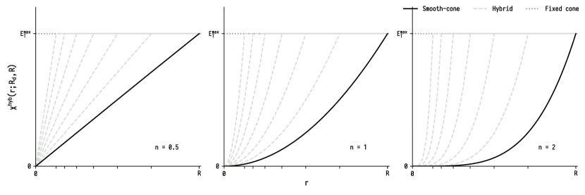
Figure 1: The matched-hybrid isolation profile function $\chi^{\text{hyb}}$ for $n\in\left\{\frac{1}{2},1,2\right\}$ and several choices of the inner cone radius, $R_{d}$ (dashed). As $R_{d}\to 0$ (dotted), the smooth-cone (solid) suppression of the collinear singularity is retained, but the numerical deviation from the constant profile function of fixed-cone isolation is diminished. For all values of $R_{d}$, exactly-collinear radiation is vetoed.

Since we are concerned with the physical criterion in eq. 8, we consider the hybrid-isolation cross-section relative to the corresponding smooth-cone prediction,

$$\Delta\sigma\left(R_{d}\right)=\sigma_{\text{hybrid}}-\sigma_{\text{smooth}},$$ (10)

using the profile function of eq. 5. We can consider $\Delta\sigma\left(R_{d}\right)$ as the physical cross-section resulting from the presence of the generalised isolation measurement function

$$\Theta\left[\chi^{\text{hyb}}\left(\left\{p_{i}\right\};\,R_{d}\right)-E_{\mathrm{T}}^{\text{had}}(R)\right]-\Theta\left[\chi^{\text{smooth}}\left(\left\{p_{i}\right\}\right)-E_{\mathrm{T}}^{\text{had}}(R)\right].$$ (11)

in the integrand. This is zero for, and hence vetoes, events that are treated commonly by the two isolation criteria, and, since $\chi^{\text{hyb}}(r;R_{d},R)\geqslant\chi^{\text{smooth}}(r;R)$ selects those that are vetoed under smooth-cone isolation but permitted under hybrid isolation. The Heaviside step functions implementing the isolation criteria induce discontinuities in the resulting distributions, which will be discussed further in section 2.2.

We begin by summarising the $R_{d}$-dependence of $\Delta\sigma\left(R_{d}\right)$, where other parameters are fixed, so $R$ and $E_{\mathrm{T}}^{{\text{thr.}}}$ are common to both profile functions. Where a gluon is emitted inside the cone,

$$\Delta\sigma\left(R_{d}\right)\sim n(R^{2}-R_{d}^{2})$$ (12)

in accordance with the intuition that the additional cross-section allowed is proportional to the area over which the gluon can additionally be emitted, which is the difference in areas between the outer and the inner cone. Where a quark is emitted, the collinear behaviour of the splitting function gives

$$\Delta\sigma\left(R_{d}\right)\sim\log\frac{R}{R_{d}}.$$ (13)

This behaviour is verified at NLO in fig. 2. The dependence of the inner-smooth-cone cross-section on its remaining isolation parameters is unchanged from the detailed description in Catani:2018krb , whilst the $R$-dependence of the outer cone is that of fixed-cone isolation as described in Catani:2013oma .

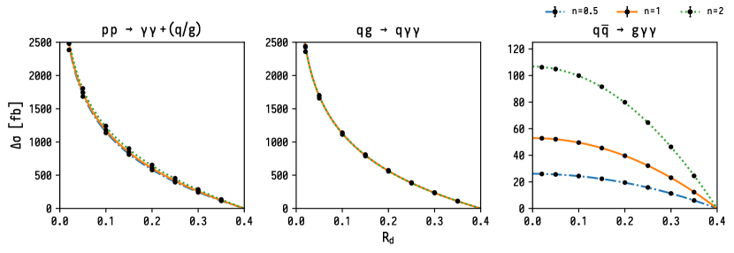
Figure 2: The variation $\Delta\sigma\left(R_{d}\right)=\sigma_{\text{hybrid}}-\sigma_{\text{smooth}}$ at NLO as a function of the inner-cone radius $R_{d}$, for $R=0.4$. All other parameters are kept constant. As expected, the gluon splitting gives rise to a quadratic dependence, whilst the quark splitting gives rise to a logarithmic divergence arising from the integrated collinear singularity.

The $\log{R}/{R_{d}}$ scaling of eq. 13 indicates that the cross-section diverges in the small-inner-cone limit, as can be seen in fig. 2, and as expected from the above discussion. This is a known feature of narrow-cones in both smooth- and fixed-cone isolation Catani:2002ny . It arises because the partition of phase-space into a cone of radius $R$ and its complement induces $\log R$ contributions in both, which cancel in their sum. Any isolation procedure applied only inside the photon cone changes the former but not the latter, leading to a miscancellation of logarithms, the remainder of which will become large in the small-$R$ limit.

We must therefore be careful to choose a value of $R_{d}$ that is large enough to regulate the collinear singularity, but small enough to approximate the fixed-cone result better than the smooth-cone value $R_{d}=R$. Ideally, this would be approximately equal to that at which the compensation that was discussed above occurs, to reproduce the cross-section given by fixed-cone isolation.

To determine the value of $R_{d}$ at which this compensation occurs, in Amoroso:2020lgh we compared NLO cross-sections and differential distributions obtained at fixed order with hybrid isolation to those obtained using Diphox with fixed-cone isolation. Diphox Binoth:1999qq is a Monte Carlo event generator implementing the NLO QCD corrections to diphoton production, together with the single- and double-fragmentation contributions. We found that for the ATLAS-motivated cuts $E_{\mathrm{T}}^{{\text{thr.}}}=11~{}\mathrm{GeV}$, $R=0.4$ and $R_{d}=0.1$ the hybrid isolation result was almost fully contained within the Diphox uncertainty band, except where the fragmentation contribution populated regions of phase-space that first enter the fixed-order calculation at the subsequent order of perturbation theory.

At NLO the underlying kinematics restrict the relevance of photon isolation to a relatively minor region of phase-space. The only part of the fixed-order NLO calculation sensitive to the isolation parameters is the real emission, and within the real contribution, the final state parton $p_{1}$ may only enter the isolation cone of the second-hardest photon, as they must together balance $\mathbf{p}_{\mathrm{T}}^{\gamma_{1}}$. The collinear invariant being regulated by the isolation criterion is therefore

$$s_{\gamma_{2}p_{1}} \approx E_{\mathrm{T}}^{{\gamma_{2}}}\,E_{\mathrm{T}}^{{1}}\;\Delta R_{\gamma_{2}p_{1}}^{2}=E_{\mathrm{T}}^{{\gamma_{2}}}\,p_{\mathrm{T}}^{\gamma\gamma}\;\Delta R_{\gamma_{2}p_{1}}^{2},$$ (14)

where

$$p_{\mathrm{T}}^{\gamma\gamma}=\left\|\mathbf{p}_{\mathrm{T}}^{\gamma_{1}}+\mathbf{p}_{\mathrm{T}}^{\gamma_{2}}\right\|$$ (15)

is the transverse momentum of the diphoton system, and the last equality is valid only for three-particle final-states.

For any monotonic profile function $\chi$, it follows from eq. 8 that the resulting isolation criterion is at least as restrictive as fixed-cone isolation with the same boundary condition, so the effect of isolation will be confined to $p_{\mathrm{T}}^{\gamma\gamma}=E_{\mathrm{T}}^{{1}}\leqslant E_{\mathrm{T}}^{\text{iso}}(\gamma_{2})$ purely from kinematic constraints. This implies that any differences between two isolation schemes are only resolved at this order on the strip

$$p_{\mathrm{T}}^{\gamma_{2}}\in\left[\max\left\{p_{\mathrm{T}}^{\gamma_{2,\mathrm{cut}}},\frac{p_{\mathrm{T}}^{\gamma_{1}}-E_{\mathrm{T}}^{{\text{thr.}}}}{1+\varepsilon_{\gamma}}\right\},\;p_{\mathrm{T}}^{\gamma_{1}}\right].$$ (16)

For asymmetric photon cuts with a $p_{\mathrm{T}}^{\mathrm{cut}}$-gap greater than $E_{\mathrm{T}}^{{\text{thr.}}}$, this would exclude events close to the threshold of the photon cuts from isolation dependence entirely, at this order. For the more conventional case, the dependence of the NLO cross-section on the parameters is dominated by events on the threshold of the cuts.

In figs. 3 and 4 we show a selection of differential cross-sections $\mathrm{d}\Delta\sigma(R_{d})/\mathrm{d}X$ for a range of values for $R_{d}$ to illustrate the distributional counterparts to fig. 2. As in fig. 2, the cuts are chosen to match those used in the 8 TeV ATLAS study, whilst the theory parameter $R_{d}$ is varied.

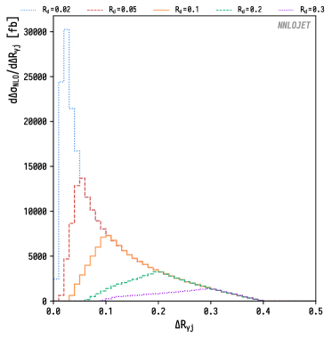
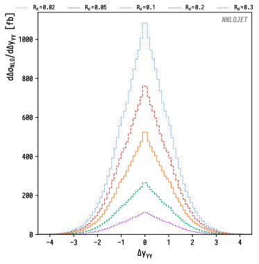
Figure 3: Isolation cone effects at NLO, showing the difference between matched-hybrid and smooth-cone isolation $\Delta\sigma$. The $\mathrm{d}\Delta\sigma/\mathrm{d}\Delta R_{\gamma j}$ distribution has regions of highly-local sensitivity to $R_{d}$, whilst the $\mathrm{d}\Delta\sigma/\mathrm{d}\Delta y_{\gamma\gamma}$ distribution is sensitive only through a small global normalisation. In the first plot the jet cut is 1 GeV; at this order all jets comprise a single parton. Higher values of the jet cut increase the minimal value of $\Delta R_{\gamma j}$ at which partons of that $p_{\mathrm{T}}$ can be emitted and not vetoed, with the minimum approximately $R\sqrt{p_{\mathrm{T}}^{j}/E_{\mathrm{T}}^{\text{iso}}}$, leading to steeper slopes to the left of the peak.

As can be seen in the first plot of fig. 3, the characteristic kinematic configuration of the events additionally allowed by hybrid isolation is very sensitive to the choice of $R_{d}$. The peak at $R_{d}$ arises because the difference between the smooth-cone and hybrid profile functions is maximised at $R_{d}$. This leads to a localised sensitivity to the $R_{d}$ parameter in certain distributions. This exposure of the collinear singularity shown in fig. 3 with decreasing $R_{d}$ illustrates the kinematics underlying the logarithmic behaviour of eq. 13, and shows a gradual bias within the photon-cone towards increasingly collinear events as the inner-cone is reduced in size. In other distributions such as $\mathrm{d}\Delta\sigma/\mathrm{d}\Delta y_{\gamma\gamma}$, also shown in fig. 3, the logarithmic behaviour manifests itself only as a global normalisation.

Further distributions in which the effect is localised are shown in fig. 4 alongside the corresponding smooth-cone distributions. These illustrate interesting features of the isolated differential cross-sections at NLO. In the first figure, the $\mathrm{d}\Delta\sigma/\mathrm{d}p_{\mathrm{T}}^{\gamma\gamma}$ distribution shows a discontinuity at $p_{\mathrm{T}}^{\gamma\gamma}=E_{\mathrm{T}}^{\text{iso}}$. The shape of this distribution is sensitive to the parameters of hybrid isolation and the offset between asymmetric photon cuts. Here, the peak occurs at the offset whilst the discontinuity occurs at $E_{2}$, in the notation of eq. 9 (including for non-matched isolation). If $E_{2}$ were allowed to depend on $p_{\mathrm{T}}^{\gamma_{2}}$ this discontinuity would be smoothed over an interval in $p_{\mathrm{T}}^{\gamma\gamma}$, but would reappear in another distribution. This arises directly from the boundary of the fixed-cone criterion in phase-space and will be discussed further, including its consequences for higher-orders, in section 2.2.

The $\mathrm{d}\Delta\sigma/\mathrm{d}p_{\mathrm{T}}^{\gamma_{2}}$ distribution, and as a direct consequence, the $\mathrm{d}\Delta\sigma/\mathrm{d}M_{\gamma\gamma}$ distribution, show discontinuities, in the differential cross-section and its derivative respectively, at the boundaries of the Born phase-space. The latter was analysed in Catani:2018krb . The former arises because real soft QCD radiation is kinematically restricted to arise only close to the back-to-back configuration $p_{\mathrm{T}}^{\gamma_{2}}\lesssim p_{\mathrm{T}}^{\gamma_{1}}$, which is permitted by the isolation criteria by design, and cannot cancel as anticipated against virtual poles outside the Born kinematics.

These (unphysical) features arise commonly in both smooth-cone and fixed-cone isolation. They are a direct consequence of the requirement that soft gluon radiation be permitted, to allow the general cancellation of real and virtual singularities. Where the virtual singularities are kinematically prohibited, but real soft singularities are not, a miscancellation arises.

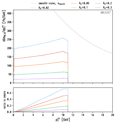
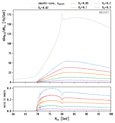
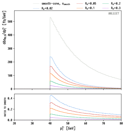
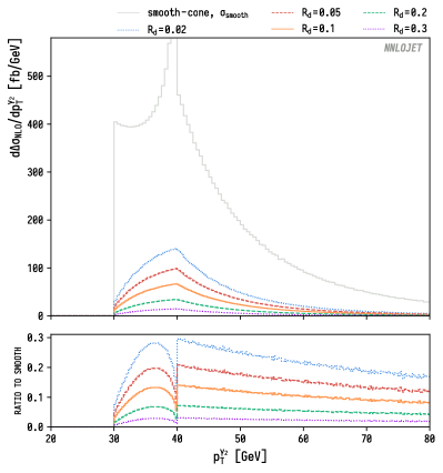
Figure 4: Detailed isolation cone effects at NLO, showing the difference between matched-hybrid and smooth-cone isolation $\Delta\sigma$. The absolute predictions for smooth-cone isolation are shown for reference. At this order, isolation criteria only apply at all in the limited region of phase-space defined by $p_{\mathrm{T}}^{\gamma\gamma}\leqslant E_{\mathrm{T}}^{\text{iso}}$. Here, as for the ATLAS 8 TeV data considered throughout, $E_{\mathrm{T}}^{\text{iso}}=11~{}\mathrm{GeV}$.

Figure 5: The variation $\Delta\sigma\left(R_{d}\right)=\sigma_{\text{hybrid}}-\sigma_{\text{smooth}}$ at NNLO as a function of the inner-cone radius $R_{d}$, for $R=0.4$. All other parameters are kept constant. The two channels not shown, ${q}{\bar{q}}$ and ${g}{g}$, have comparable shape (but smaller magnitude) to ${q}{g}$ and ${q}{q}$ respectively.

Since the behaviour of the isolated cross-section at NLO is highly sensitive to the unphysical behaviour in these regions, it is a priori unclear to what extent the variation of isolation parameters based on NLO behaviour will lead to conclusions that hold at higher orders. Running enough calculations at NNLO with sufficient resolution to investigate the $R_{d}$-dependence of distributions in the regions of non-analyticity shown in fig. 4 would be prohibitively computationally expensive. In section 2.3 we therefore compare smooth-cone isolation to matched-hybrid isolation with fixed $R_{d}=0.1$.

To illustrate the overall dependence of the NNLO cross-section on $R_{d}$, in fig. 5 we show the NNLO counterpart to fig. 2. The dependence on $R_{d}$ is again dominated by the ${q}{g}$ channel. Overall, the magnitude of the effect is similar to that at NLO despite the contribution from events outside the strip of eq. 16, whilst the shape is no longer logarithmic. Channels in which a parton is permitted to enter the photon cone for the first time at NNLO have the same $R_{d}$-dependence shown in fig. 2. This suggests that the procedure used to justify the choice $R_{d}=0.1$ above, by comparison to the fragmentation calculation, should remain valid at NNLO.

The $R_{d}$-dependence illustrated in figs. 2 and 5 can be used to estimate the uncertainty resulting from the choice of $R_{d}=0.1$. This uncertainty does not arise directly from hybrid isolation, but rather from the inherent uncertainty in the freedom to choose a profile function within generalised smooth-cone isolation. The hybrid-isolation profile function parametrises the local regulation of the collinear singularity directly, allowing this uncertainty to emerge from parameter variation, unconstrained by the properties of the profile function far from the collinear point $r=0$. Twofold variation in $R_{d}$ about $R_{d}=0.1$ gives an uncertainty band of approximately 1000–1500$\mathrm{fb}$ for both NLO and NNLO, smaller than that induced by scale variation at the corresponding order and so of comparable magnitude to the general theory uncertainty we assign to the calculation.

The natural comparison of these isolation uncertainties is with the fragmentation uncertainty that would arise within a fragmentation-inclusive calculation in which the collinear singularity is absorbed via a mass factorisation counterterm. This will eliminate the $R_{d}$-dependence of the hybrid-isolation predictions, but at the expense of introducing a sensitivity to photon fragmentation functions, which are only loosely constrained by current experimental data. Such a comparison cannot yet be made at NNLO, and must be postponed until such a calculation has been completed. As at NLO, we expect that the NNLO calculation using hybrid isolation should coincide with the fragmentation-inclusive calculation at the same order for some finite positive value of $R_{d}$, and its associated uncertainty can be assessed by a variation around this value.

In practice we limit the exposure of the hybrid-isolation cross-section to the $R_{d}\to 0$ limit through the ‘perturbative unitarity’ heuristic argument outlined above, using the constraints imposed by fragmentation at NLO. Since the $R_{d}$-dependence at NNLO seems to be dominated by the NLO real-radiation effects, we can reasonably expect this heuristic argument to limit the possible size of deviation between fragmentation-inclusive and hybrid-cone isolated cross-sections just as it does at NLO, and to approximate the uncertainty inherent to the limited knowledge on the fragmentation process.

2.2 Infrared sensitivity

In general, any parton-level cone-based isolation criterion of the generic form eq. 3 amounts to a veto implemented through a measurement function containing factors of the form

$$\prod_{\gamma}\prod_{i=1}^{n}\;\mathcal{I}_{\gamma i},$$ (17)

where the index $i$ ranges over final-state partons, and

$$\mathcal{I}_{\gamma i}=\Theta\left[E_{\mathrm{T}}^{\text{iso}}(\gamma)\;\chi\left(\min\left(\Delta R_{\gamma i},R\right);R\right)-\sum_{j=1}^{n}E_{\mathrm{T}}^{{j}}\;\Theta\left[\min\left(\Delta R_{\gamma i},R\right)-\Delta R_{\gamma j}\right]\right]$$ (18)

(using the $\Theta(0)=1$ convention). This is zero, and hence vetoes events, in which the accumulated partonic energy in the cone exceeds the profile function.

It can readily be seen from this formalism that the Heaviside step function implies a discontinuity in the integrand at the bounding surface on which the isolation criteria inequalities are exactly saturated. This is an intrinsic property of veto-based isolation techniques. At NLO, where there is a single parton that can only enter the photon cone of the softer photon, the consequences of this become clearer:

$$\mathcal{I}_{\gamma 1}=\Theta\left[E_{\mathrm{T}}^{\text{iso}}(\gamma)\;\chi\left(\min\left(\Delta R_{\gamma 1},R\right);R\right)-E_{\mathrm{T}}^{{1}}\;\Theta\left[\min\left(\Delta R_{\gamma 1},R\right)-\Delta R_{\gamma 1}\right]\right]$$ (19)

That is, we expect to have introduced a step-like discontinuity inside the physical region at

$$p_{\mathrm{T}}^{\gamma\gamma}\equiv E_{\mathrm{T}}^{{1}}=E_{\mathrm{T}}^{\text{iso}}(\gamma)\;\chi\left(\Delta R_{\gamma 1};R\right)\qquad\forall\Delta R_{\gamma 1}\leqslant R$$ (20)

where the integrand is zero for $p_{\mathrm{T}}^{\gamma\gamma}>E_{\mathrm{T}}^{\text{iso}}(\gamma)\;\chi\left(\Delta R_{\gamma 1};R\right)$ and non-zero below it, through the formulation of the isolation criterion. This is precisely the source of the discontinuity visible in fig. 4. For the complementary region $\Delta R_{\gamma 1}>R$ where the parton is outside the cone, there is no discontinuity in the integrand: the measurement function eq. 19 is never zero, and so the isolated and unisolated integrands are identical everywhere. Conversely, examining instead the region defined by $p_{\mathrm{T}}^{\gamma\gamma}\geqslant E_{\mathrm{T}}^{\text{iso}}(\gamma)$ we see the same step-like discontinuity arising at $\Delta R_{\gamma 1}=R$, the boundary of the isolation cone.

Such discontinuities within the physical region were first described in general in Catani:1997xc . For diphoton production they first arise in the NLO-plus-fragmentation calculation and were remarked upon in Binoth:1999qq , but have not previously been identified in the NNLO direct production calculation. They represent a localised breakdown of perturbation theory in which a step-like discontinuity leads at higher orders to infrared Sudakov singularities. These arise from the disruption of the expected cancellation between soft real gluons and the corresponding virtual corrections, since isolation vetoes a subset of the former without affecting the latter. Resummation of the generated logarithms is then expected to restore continuity of the distribution, resulting in a characteristic ‘Sudakov shoulder’. Following the logic outlined in Catani:1997xc , the step-like isolation behaviour shown in fig. 4 leads to a double-logarithmic divergence in the region $p_{\mathrm{T}}^{\gamma\gamma}<E_{\mathrm{T}}^{{\text{thr.}}}$,

$$\Delta^{\pm}_{p_{\mathrm{T}}^{\gamma\gamma}=E_{\mathrm{T}}^{{\text{thr.}}}}\sim-\ln^{2}\left[1-\left(\frac{p_{\mathrm{T}}^{\gamma\gamma}}{E_{\mathrm{T}}^{{\text{thr.}}}}\right)^{2}\right].$$ (21)

This behaviour does indeed arise in the NNLO $\mathrm{d}\sigma/\mathrm{d}p_{\mathrm{T}}^{\gamma\gamma}$ distribution as expected. It is shown alongside the corresponding NLO discontinuity in fig. 6, together with the corresponding (continuous) smooth-cone distribution. The distinctive double-singularity shape of the hybrid-isolation distribution is as anticipated in Catani:1997xc , and represents a clear deviation from the expected behaviour of the hybrid-isolation distribution on physical grounds from eq. 8.

There is an additional Sudakov critical point arising from the boundary of the Born kinematic region at $p_{\mathrm{T}}^{\gamma\gamma}=0$ which would also be expected to require resummation to generate reliable predictions. The practical effect of this additional singularity at small $p_{\mathrm{T}}^{\gamma\gamma}$ is therefore to revise upwards the lower boundary of the region of the $p_{\mathrm{T}}^{\gamma\gamma}$-distribution at which we might expect NNLO calculations to accurately describe the data. For current experimental binnings, this effect is negligible. The singularities are integrable, and the positive and negative logarithmic contributions typically cancel against each other in a single bin that contains the critical point. However, as the target precision of both experimental data and theoretical predictions increases, these effects may not remain negligible, especially if a bin-edge coincides with the Sudakov critical point.

We briefly remark on the second discontinuity implied by eq. 19, in the $\Delta R_{\gamma j}$ distribution. The NLO isolation function eq. 19 implies a discontinuity in $\Delta R_{\gamma 1}$ at the boundary of the isolation cone. At NLO, where each identified jet comprises a single parton, this would lead to a discontinuity in a $\Delta R_{\gamma_{2}j_{1}}$ distribution, were the jet definition set small enough to allow partons to be simultaneously soft enough to be permitted inside the cone by isolation, and hard enough to be identified as a jet. The obvious tension between these two conditions makes this a theoretical, rather than a phenomenological concern. At NNLO, however, the possibility arises for partons soft enough to be permitted inside the cone by the isolation criteria to be combined with harder partons outside the cone, resulting in a jet with $\Delta R_{\gamma j}>R$. The underlying discontinuity at one order and the resulting Sudakov singularities at the next order would then be displaced relative to one another, and would resemble a new phenomenon of unclear origin. These boundary effects can be expected to lead to unphysical results in any fixed-order prediction of photon-jet separation.

At NLO, the nature of the isolation-induced discontinuity shown in fig. 4 is specific to hybrid- and fixed-cone isolation with $\varepsilon_{\gamma}=0$. The surface defined in eq. 19 is a surface of constant $p_{\mathrm{T}}^{\gamma\gamma}$, and hence the discontinuity introduced into the integrand remains in the $\mathrm{d}\sigma/\mathrm{d}p_{\mathrm{T}}^{\gamma\gamma}$ distribution, and at higher orders gives rise to a Sudakov critical point. More generally, for $\varepsilon_{\gamma}=0$ a discontinuity in the $p_{\mathrm{T}}^{\gamma\gamma}$-distribution arises from any interval on which $\chi(r;R)$ is constant.

The discontinuity is fully regulated in smooth-cone isolation in NLO kinematics, since the boundary in $p_{\mathrm{T}}^{\gamma\gamma}$ at which the discontinuity would arise is no longer a constant $E_{\mathrm{T}}^{{\text{thr.}}}$, but a monotonic function of $r$, and the threshold of permitted events is spread evenly across $p_{\mathrm{T}}^{\gamma\gamma}$ rather than discretely at a boundary. This masks the IR critical point and gives a smooth $p_{\mathrm{T}}^{\gamma\gamma}$ distribution. However, it instead introduces one into the $p_{\mathrm{T}}^{\gamma\gamma}/\chi(r)$ distribution.

Within hybrid isolation, continuity can be restored to the $p_{\mathrm{T}}^{\gamma\gamma}$-distribution by, for example, introducing a small non-zero $\varepsilon_{\gamma}$. This amounts to a rotation of the boundary surface, and moves the discontinuity from the $p_{\mathrm{T}}^{\gamma\gamma}$-distribution into the $(p_{\mathrm{T}}^{\gamma\gamma}-\varepsilon_{\gamma}p_{\mathrm{T}}^{\gamma_{2}})$ distribution. The resulting Sudakov singularities in the latter distribution then manifest themselves in the $p_{\mathrm{T}}^{\gamma\gamma}$ distribution as an unphysical bump resulting from the remainder of the cancellation of positive and negative Sudakov logarithms in each bin.

These discontinuities, and the resulting singularities, are therefore a necessary consequence of cone-based isolation, and can only be moved between distributions, rather than avoided entirely. The effect of the logarithms is not confined to the distribution that is discontinuous at a lower order, but can leak into correlated distributions, where it may be harder to identify.

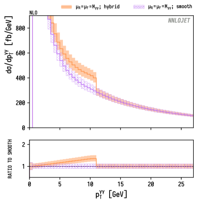
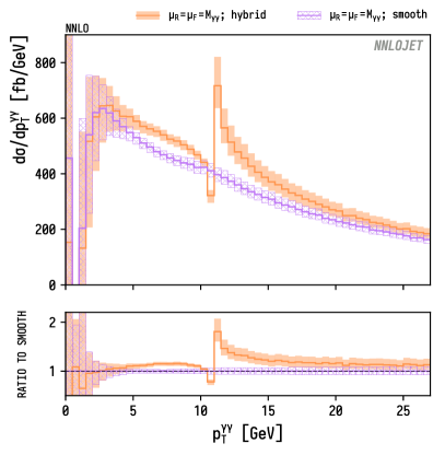
Figure 6: Discontinuity in the $\mathrm{d}\sigma/\mathrm{d}p_{\mathrm{T}}^{\gamma\gamma}$ distribution arising from hybrid isolation at NLO with $E_{\mathrm{T}}^{{\text{thr.}}}=11\mathrm{GeV}$, and the resulting Sudakov singularity at NNLO.

In general, any observable whose definition is constructed to align with the axis of the step-function will exhibit this threshold behaviour. Where this coincides at a lower order with an observable of physical interest, it is likely to lead to infrared sensitivity. For sufficiently wide histogram bins (including those used for the ATLAS 8 TeV data), the integrable singularities are masked, whilst binnings that combine both critical points, at $p_{\mathrm{T}}^{\gamma\gamma}=0$ and $p_{\mathrm{T}}^{\gamma\gamma}=E_{\mathrm{T}}^{{\text{thr.}}}$ into a single bin disguise both Sudakov critical points entirely, as in fig. 13 of Catani:2018krb .

Given this, it appears that the phenomenological significance of these singularities is limited, provided that deviations from fixed-order predictions in these regions are not misunderstood to have physical significance. This is easier to recognise in distributions such as $p_{\mathrm{T}}^{\gamma\gamma}$ that are directly constrained by photon isolation than it might be where the analogous observable is not of direct physical interest. This is the case, for example, for the photon-plus-jet process, where different experimental cuts and attention to different observables change the relevance of the expected non-analytic behaviour of $p_{\mathrm{T}}^{\gamma j}$.

However, for colourless final-states including the diphoton final state, the differential cross section with respect to the transverse momentum of the identified final state has particular significance, as it is relied upon by alternative subtraction schemes such as $q_{\mathrm{T}}$- or $N$-jettiness subtraction. It is clear from fig. 6 that the $p_{\mathrm{T}}^{\gamma\gamma}$-dependence of the cross-section at small $p_{\mathrm{T}}^{\gamma\gamma}$ is sensitive to the details of the isolation used and not universal, which would explain the absence of a plateau in the $r_{\mathrm{cut}}$-dependence plots for diphoton production using $q_{\mathrm{T}}$-subtraction with Matrix in Grazzini:2017mhc . These power corrections have been explored analytically in Ebert:2019zkb , where it was found that for smooth-cone isolation, they grow in magnitude as $\left({Q}/{E_{\mathrm{T}}^{\text{iso}}}\right)^{{1}/{n}}$, with a proposal for how they could be accounted for. As a result, the phenomenological significance of these power corrections should grow as we move to higher centre-of-mass energies. It remains to be seen whether they will pose a meaningful problem for these alternative subtraction schemes.

2.3 Comparison of hybrid and smooth-cone distributions

We now outline the key differences of phenomenological significance between hybrid and smooth-cone isolation, as applied to a selection of differential cross-sections. We use a setup corresponding to the ATLAS 8 TeV data Aaboud:2017vol , which we will return to in section 4.1, and plot data for those distributions where it exists for later reference. The relevant fiducial cuts are:

$$p_{\mathrm{T}}^{\gamma_{1}} >40\;\mathrm{GeV}\,, p_{\mathrm{T}}^{\gamma_{2}} >30\;\mathrm{GeV}\,,$$ (22a)

$$\Delta R_{\gamma\gamma} >0.4\,, \left|y^{\gamma}\right| \in\left[0,1.37\right)\cup\left(1.56,2.37\right),$$ (22b)

$$E_{\mathrm{T}}^{\text{iso,part}} <11\;\mathrm{GeV} \text{within cone}\enspace\Delta R \leqslant 0.4.$$ (22c)

We choose $R_{d}=0.1$ for hybrid isolation, as outlined in section 2.1, and smooth-cone isolation parameters $n=1$ and $E_{\mathrm{T}}^{\text{iso}}=11~{}\mathrm{GeV}$ for both $\chi$ and $\chi^{\text{hyb}}$. Here and throughout we use the NNPDF 3.1 parton distribution functions Ball:2017nwa . The QED coupling constant $\alpha$ is set at $\alpha_{\mathrm{em}}(0)=1/137$.

We first explore the effect of moving from smooth-cone to hybrid isolation on differential cross-sections chosen to illustrate the underlying features.

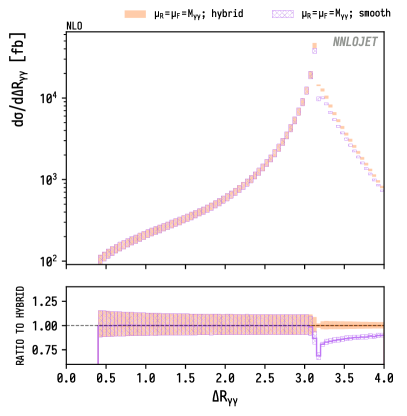
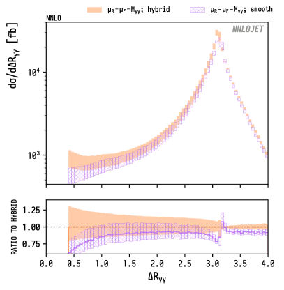
(a) $\Delta R_{\gamma\gamma}$ at NLO and NNLO using matched-hybrid and smooth-cone isolation.

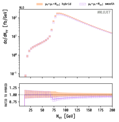
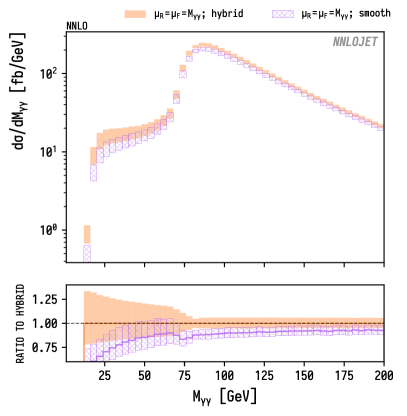
(b) The induced effects at low $\Delta R_{\gamma\gamma}$ on $M_{\gamma\gamma}$.

Figure 7: $\mathrm{d}\sigma/\Delta R_{\gamma\gamma}$ and $\mathrm{d}\sigma/M_{\gamma\gamma}$ at NLO and NNLO using matched-hybrid and smooth-cone isolation. The deviations for small $M_{\gamma\gamma}$ and $\Delta R_{\gamma\gamma}$ are related, as events with small $M_{\gamma\gamma}$ can only both pass the photon cuts if they have sufficiently small $\Delta R_{\gamma\gamma}$. For example, for these cuts, $M_{\gamma\gamma}\leqslant 27~{}\mathrm{GeV}$ requires $\Delta R_{\gamma\gamma}\leqslant 0.8$.

In fig. 7 we show $\mathrm{d}\sigma/\mathrm{d}\Delta R_{\gamma\gamma}$ and $\mathrm{d}\sigma/\mathrm{d}M_{\gamma\gamma}$. The relative enhancement is greatest at low $M_{\gamma\gamma}$, whilst the absolute enhancement $\mathrm{d}\Delta\sigma/\mathrm{d}M_{\gamma\gamma}$ follows the shape of the underlying distribution, with the difference largest at the Born threshold of $M_{\gamma\gamma}=80~{}\mathrm{GeV}$. Broadly these reflect the two dominant configurations in which soft partonic emissions can enter into isolation cones: either the photons are balanced against each other (Born-like), or the diphoton system is relatively collimated and balanced against a jet. Accordingly, configurations with the explicit requirement of an extra jet see a further peak in $\mathrm{d}\Delta\sigma/\mathrm{d}M_{\gamma\gamma}$ at $M_{\gamma\gamma}\approx p_{\mathrm{T}}^{j_{\mathrm{cut}}}$ corresponding to $\Delta R_{\gamma\gamma}\approx\Delta R_{\gamma\gamma}^{\mathrm{cut}}$, as shown in fig. 8. In the $p_{\mathrm{T}}^{j_{\mathrm{cut}}}\to 0$ limit, this is effectively truncated by the cuts on $\Delta R_{\gamma\gamma}$, which is the configuration corresponding to the small $\Delta R_{\gamma\gamma}$ effects seen in fig. 7. As the jet cut increases this peak will become dominant.

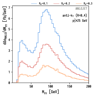
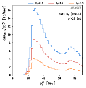
Figure 8: The absolute difference between the hybrid- and smooth-cone isolation differential cross-sections $\mathrm{d}\sigma/\mathrm{d}M_{\gamma\gamma}$ and $\mathrm{d}\sigma/\mathrm{d}p_{\mathrm{T}}^{\gamma\gamma}$ for $R_{d}=0.1,0.2,0.3$, for diphoton production in association with an anti-$k_{\mathrm{T}}$ jet of $p_{\mathrm{T}}{}\geqslant 25\;\mathrm{GeV}$, with $R=0.4$.

The requirement of a jet imposes a lower bound on $p_{\mathrm{T}}^{\gamma\gamma}$ and so removes the Sudakov instabilities of the inclusive distribution that were discussed in section 2.2. The two peaks in the two plots correspond to the same physics in the opposite order, with the peak at $p_{\mathrm{T}}^{\gamma\gamma}\approx p_{\mathrm{T}}^{j_{\mathrm{cut}}}$ corresponding to the configuration in which the photons and jet are balanced, and the second peak at $p_{\mathrm{T}}^{\gamma\gamma}\approx 75\,\mathrm{GeV}$ corresponding to the threshold at 70 GeV, the smallest value that can be generated within the cuts for every value of $\Delta\phi_{\gamma\gamma}$. As discussed in Binoth:2000zt ; Catani:2018krb , below this threshold the photon cuts imply an implicit minimum for $\Delta\phi_{\gamma\gamma}$, restricting the available phase-space. Contributions from this peak give rise to a distinctive cusp in both the experimental and the NNLO distributions which, corresponding to the small-$\Delta R_{\gamma\gamma}$ region, is especially sensitive to isolation. Smooth-cone isolation suppresses the kinematic peak in this region, which is restored by the less restrictive hybrid isolation profile function.

Finally, for completeness, in fig. 9 we consider four further differential cross-sections of interest. The $p_{\mathrm{T}}^{\gamma_{1}}$ and $p_{\mathrm{T}}^{\gamma_{2}}$ distributions are affected most substantially at the boundary of the photon cuts, as expected from fig. 4, but are elsewhere mostly unchanged by modifications of the cuts. These regions dominate the cross-section, and explain the large $R_{d}$-sensitivity of fig. 5. Whether the correction here is purely physical or, particularly for the $p_{\mathrm{T}}^{\gamma_{2}}$ distribution, arises from unphysical behaviour at the boundary of the Born phase-space, is unclear. As at NLO, for the rapidity separation $\Delta y_{\gamma\gamma}$ the additional events permitted by hybrid isolation amount to an overall constant factor in $\mathrm{d}\Delta\sigma/\mathrm{d}\Delta y_{\gamma\gamma}$.

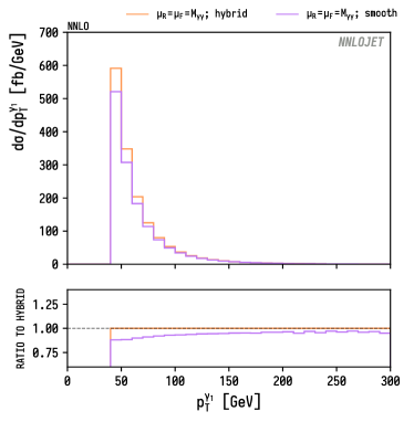
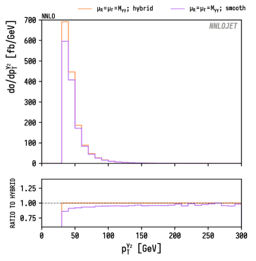
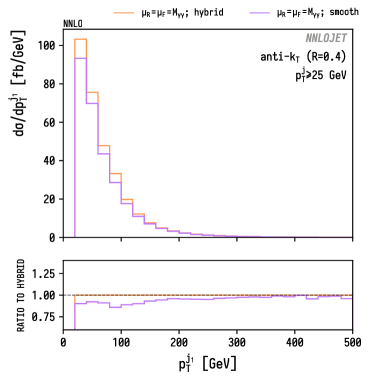
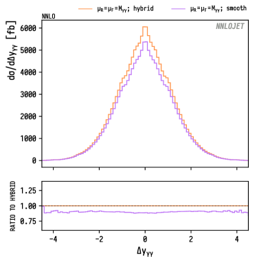
Figure 9: The NNLO distributions $\mathrm{d}\sigma/\mathrm{d}p_{\mathrm{T}}^{\gamma_{1}}$, $\mathrm{d}\sigma/\mathrm{d}p_{\mathrm{T}}^{\gamma_{2}}$, $\mathrm{d}\sigma/\mathrm{d}p_{\mathrm{T}}^{j_{1}}$ and $\mathrm{d}\sigma/\mathrm{d}\Delta y_{\gamma\gamma}$ for hybrid-cone and smooth-cone isolation respectively, and the ratio between the smooth-cone and the hybrid distributions. The defining jet requirement for the third plot is of an anti-$k_{\mathrm{T}}$ jet with $p_{\mathrm{T}}^{j}\geqslant 25\mathrm{GeV}$ and $R=0.4$.

In this section we have compared smooth-cone to hybrid isolation at NNLO for a range of differential cross-sections of phenomenological significance. The effect of interchanging them, which indicates the uncertainty associated to the theoretical implementation of the isolation criteria, is substantial and leads to effects of approximately 10% in uncorrelated distributions, and localised effects of up to 40% in distributions highly sensitive to the specifics of the isolation criteria. Uncertainties of this magnitude are compatible with the size of the scale-uncertainty band, and therefore represent a substantial theory uncertainty that should be accounted for.

We will return to consider isolation effects in tandem with scale choice in section 4.

3 Scale choice

A further uncertainty in the theoretical calculation arises from the choice of functional form $\mu_{0}$ for the renormalisation and factorisation scales. The conventional choice is $\mu_{0}=M_{\gamma\gamma}$, the invariant mass of the diphoton system, with the magnitude of missing higher-order-uncertainties (MHOUs) estimated through the envelope of the variation $\mu_{\mathrm{R},\mathrm{F}}=\xi_{\mathrm{R},\mathrm{F}}\cdot\mu_{0}$ for $\xi_{\mathrm{R}},\xi_{\mathrm{F}}\in\left\{\frac{1}{2},1,2\right\}$.

Where two a priori reasonable choices of $\mu_{0}$ themselves differ by a factor greater than 2, either locally or globally, this procedure fails to span the uncertainty of the calculation even at the known orders. Any estimate of MHOUs is therefore potentially unreliable.

We begin by briefly reviewing the common scale choices for related processes. In sections 3.2 and 3.3 we then look at the effects of moving between two choices motivated by these, $\mu_{0}=M_{\gamma\gamma}$ and $\mu_{0}=\left\langle p_{\mathrm{T}}^{\gamma}\right\rangle$, the arithmetic mean of the photon transverse momenta of the two required photons. Finally, in section 3.4 we generalise to a wider class of possible scale choices.

3.1 Scale choice for photon processes

We briefly summarise the scale choices used in the literature for this and related processes. In Binoth:1999qq , the first NLO study of diphoton production with fragmentation (Diphox), the authors used $\mu_{0}=\frac{11}{20}\left\langle p_{\mathrm{T}}^{\gamma}\right\rangle$ for fixed-target data, and $\mu_{0}=M_{\gamma\gamma}$ as the central scale for LHC predictions. This scale is also used for NNLO calculations making predictions for or comparisons with data in Catani:2011qz ; Campbell:2016yrh ; Catani:2018krb and the experimental papers applying them to measurements at the Tevatron Aaltonen:2012jd ; Abazov:2013pua and the LHC Chatrchyan:2014fsa ; Aad:2012tba ; Aaboud:2017vol . In Catani:2018krb the scale $\mu_{0}=M_{\mathrm{T}}^{\gamma\gamma}=\sqrt{M_{\gamma\gamma}^{2}+(p_{\mathrm{T}}^{\gamma\gamma})^{2}}$ is additionally considered, finding that the results differ from those for $M_{\gamma\gamma}$ only in regions of distributions that correspond to the presence of a hard, high-$p_{\mathrm{T}}$ jet.

For an inclusive single photon and a single photon in association with a jet, $p_{\mathrm{T}}^{\gamma}$ is used in the NNLO calculations of Campbell:2016lzl ; Chen:2019zmr . In the context of PDF fits, it was found in Campbell:2018wfu that direct photon production data with the former NNLO calculation and scale $p_{\mathrm{T}}^{\gamma}$ could be incorporated into the NNPDF 3.1 global fit without exhibiting tensions with other data.

For triphoton production, $M_{\gamma\gamma\gamma}$ is used for the MCFM NLO calculation in Campbell:2014yka , and $\frac{1}{4}H_{\mathrm{T}}=\frac{3}{4}\left\langle p_{\mathrm{T}}^{\gamma}\right\rangle$ and $\frac{1}{2}H_{\mathrm{T}}=\frac{3}{2}\left\langle p_{\mathrm{T}}^{\gamma}\right\rangle$ are both found to be in agreement with data in the NNLO calculation of Chawdhry:2019bji .

Finally, we note that the closest kinematically-related process whose measurements were used in the NNPDF 3.1 fit is that of single-inclusive jets, for which the jet $p_{\mathrm{T}}$ was used as the central scale. A more recent study of the scale-choice for single-inclusive jet cross-sections AbdulKhalek:2020jut used the central choice $\hat{H}_{\mathrm{T}}$, the scalar sum of the transverse momenta of all partons in the event.

This illustrates that the conventional choice for diphoton production of $\mu_{0}=M_{\gamma\gamma}$ is somewhat atypical among related processes. Its main advantage is for Higgs processes or through the analogy with dilepton final states arising from heavy-boson decay. For such processes the invariant mass of the conditioned-upon two-particle final-state particles gives the imputed invariant mass of the virtual boson. For QCD photon production, however, there is no particle to which this invariant mass is expected to correspond, and no QCD vertex with which it can be associated. To explore the significance of this convention we therefore choose to compare $\mu_{0}=M_{\gamma\gamma}$ against alternatives below, focusing on $\mu_{0}=\left\langle p_{\mathrm{T}}^{\gamma}\right\rangle$.

3.2 Perturbative convergence

We first consider the perturbative convergence of the cross-section. In fig. 10 we show the cross-section and $K$-factors at NLO and NNLO for a number of choices of dynamic scale, as well as the scale evolution calculated from the renormalisation group equations.

The NLO $K$-factors are consistently large due to the opening of the ${q}{g}$ channel, and vary according to its considerable dependence on the scale choice. The $K$-factor for the ${q}{\bar{q}}$ channel alone is approximately 1.5. The cross-sections for dynamic scale choices are largely consistent with the fixed-scale calculation corresponding to their mean value, suggesting the reweighting of phase-space by the dynamism of the dynamic central scales has a limited effect on the total cross-section. At NNLO, the $K$-factor is still considerable (approximately 1.4), due to sizeable NLO corrections in the ${q}{g}$ channel ($K$-factor ~1.3), NNLO corrections in the ${q}{\bar{q}}$ channel (~1.2), and the opening of the ${g}{g}$ and ${q}{q}^{\prime}$ channels, but is stable for all the choices of scales considered.

Overall, as expected from the running of $\alpha_{\mathrm{s}}$, dynamic scales which range over smaller values lead to larger predictions than those with larger values. Purely in terms of the distribution of their magnitude, the scales $\left\langle p_{\mathrm{T}}^{\gamma}\right\rangle$ and $M_{\gamma\gamma}$ represent the two extremes between which other reasonable dynamic scales are likely to fall.

Despite the stability of the NNLO-to-NLO $K$-factor across these choices of scales, it is clear from the gradient of the grey band that the scale-dependence remains significant. The use of a dynamic rather than a fixed scale can be seen to bring the scales into closer agreement than would be expected from their central values alone.

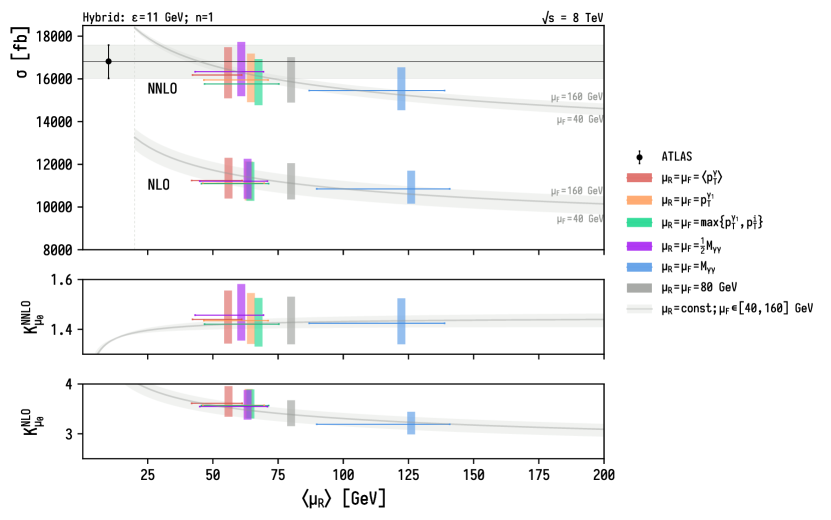
Figure 10: Scale dependence of the cross-section. Each cross-section associated with a dynamical scale $\mu_{0}$ is plotted against its mean, $\langle\mu_{0}\rangle$. The $x$-error bars indicate the lower- and upper-quartiles of the scale-variable distribution, calculated from the binned data. The scale bands are the scale uncertainties associated with the usual 7-point scale variation around the central scale. The grey bands give the cross-section for the fixed scales $\mu_{\mathrm{R}},\mu_{\mathrm{F}}$ specified, calculated from the renormalisation group equations.

3.3 Kinematic effects

We now consider the kinematics of the two scales $M_{\gamma\gamma}$ and $\left\langle p_{\mathrm{T}}^{\gamma}\right\rangle$, focusing on regions of phase-space in which we expect the ratio ${M_{\gamma\gamma}}/{\left\langle p_{\mathrm{T}}^{\gamma}\right\rangle}$ to become large (or small) and potentially lead to discrepancies arising from large logarithms of ratios of the scales. Although we focus on the diphoton context, including the ATLAS cuts, the underlying kinematic properties are universal.

In the Born kinematics, $\left\langle p_{\mathrm{T}}^{\gamma}\right\rangle=p_{\mathrm{T}}^{\gamma_{1}}=p_{\mathrm{T}}^{\gamma_{2}}$ and

$$M_{\gamma\gamma}=2\left\langle p_{\mathrm{T}}^{\gamma}\right\rangle\cosh\left(\frac{1}{2}\Delta y_{\gamma\gamma}\right)\geqslant 2\left\langle p_{\mathrm{T}}^{\gamma}\right\rangle.$$ (23)

The fiducial cuts on rapidity separation restrict $\left|\Delta y_{\gamma\gamma}\right|\leqslant 4.74$ and hence in the Born kinematics,

$$2\left\langle p_{\mathrm{T}}^{\gamma}\right\rangle\leqslant M_{\gamma\gamma}\leqslant 10.8\left\langle p_{\mathrm{T}}^{\gamma}\right\rangle.$$ (24)

Thus already at leading order, the two scales differ by at least the factor of 2 used in the conventional renormalisation and factorisation scale variation. We can therefore anticipate there to be regions of differential distributions in which the scale uncertainty bands around the two choices of $\mu_{0}$ do not overlap.

The exponential behaviour of the scale $M_{\gamma\gamma}$ at high rapidity separations persists to all orders, with the general expression

$$M_{\gamma\gamma}=\sqrt{2p_{\mathrm{T}}^{\gamma_{1}}p_{\mathrm{T}}^{\gamma_{2}}\left(\cosh\Delta y_{\gamma\gamma}-\cos\Delta\phi_{\gamma\gamma}\right)}.$$ (25)

At higher orders, $M_{\gamma\gamma}\leqslant\left\langle p_{\mathrm{T}}^{\gamma}\right\rangle$ becomes possible. $M_{\gamma\gamma}$ is bounded below only as a result of the photon separation cut $\Delta R_{\gamma\gamma}\geqslant 0.4$, which restricts

$$M_{\gamma\gamma}\geqslant 2\sqrt{p_{\mathrm{T}}^{\gamma_{1}}p_{\mathrm{T}}^{\gamma_{2}}}\sin\left(\frac{1}{2}\Delta R_{\gamma\gamma}^{\mathrm{cut}}\right)>13.76\;\mathrm{GeV}$$ (26)

for the ATLAS cuts described in eq. 22. Without this cut, which is set to be equal to the isolation cone radius by experiment specifically to exclude each photon from the isolation cone of the other, $M_{\gamma\gamma}$ would in principle be permitted within the calculation to get arbitrarily small. Thus for fixed $p_{\mathrm{T}}^{\gamma_{1}}$ and $p_{\mathrm{T}}^{\gamma_{2}}$ (and hence fixed $\left\langle p_{\mathrm{T}}^{\gamma}\right\rangle$), $M_{\gamma\gamma}$ can vary over a factor of approximately 25:

$$0.397\leqslant\frac{M_{\gamma\gamma}}{\sqrt{p_{\mathrm{T}}^{\gamma_{1}}p_{\mathrm{T}}^{\gamma_{2}}}}\leqslant 10.8,$$ (27)

with the size of this factor entirely dependent on cuts chosen for primarily experimental reasons. Were the photon-separation cut allowed to become smaller (e.g. to $\Delta R_{\gamma\gamma}\geqslant 0.2$), or the maximum rapidity separation allowed to grow (e.g. from 4.74 to 6), this ratio would span two orders of magnitude.

To illustrate the range of values taken by the ratio ${M_{\gamma\gamma}}/{\left\langle p_{\mathrm{T}}^{\gamma}\right\rangle}$ we show the corresponding normalised distribution at LO, NLO and NNLO in fig. 11. We see that the modal value for the ratio is 2, and that the regions where the logarithm of the ratio will be large are suppressed in their contribution to the cross-section, and predominantly arise from the NNLO contribution as additional partonic radiation allows the kinematic configuration to depart further from the Born.

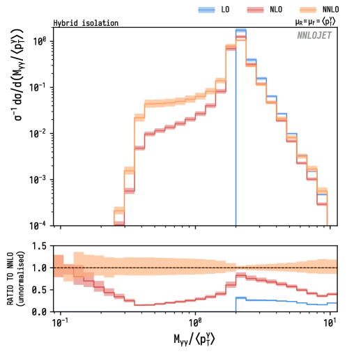
Figure 11: Ratio of scale variables. As phase-space constraints are lifted by the emission of additional partons, large ratios of scales become possible.

The distortive effect of the scale choice on differential cross-sections depends substantially on the order of the strong coupling $\alpha_{\mathrm{s}}$, through the renormalisation group equations. This is illustrated in fig. 12. The ${\mathrm{d}\sigma}/{\mathrm{d}\Delta y_{\gamma\gamma}}$ distribution exposes the exponential behaviour remarked upon in eq. 25. At leading-order $\alpha_{\mathrm{s}}^{0}$, the calculation is independent of $\mu_{\mathrm{R}}$, and so the dependence is only on $\mu_{\mathrm{F}}$ through the PDFs. The dependence is mild: the results for the scale choice $\mu_{0}=M_{\gamma\gamma}$ are modestly larger than those for $\mu_{0}=\left\langle p_{\mathrm{T}}^{\gamma}\right\rangle$, with the deviation largest for $\Delta y_{\gamma\gamma}=0$ where $M_{\gamma\gamma}=2\left\langle p_{\mathrm{T}}^{\gamma}\right\rangle$ exactly, due to eq. 23, and as can be seen through the coincidence of the scale bands of one scale with the central scale of the other.

Additional powers of the coupling constant $\alpha_{\mathrm{s}}$ reverse that hierarchy, due to the monotonicity of the running of the coupling that ensures $\alpha_{\mathrm{s}}(\mu_{1})\geqslant\alpha_{\mathrm{s}}(\mu_{2})$ for $\mu_{1}\leqslant\mu_{2}$. Thus in the regions of large rapidity-separation, the $\mu_{0}=M_{\gamma\gamma}$ predictions are suppressed relative to those for $\mu_{0}=\left\langle p_{\mathrm{T}}^{\gamma}\right\rangle$ by up to 30%.

In the extremes of the distribution, this is driven by the constructive interference of factorisation- and renormalisation-scale variation, in the sense that larger $\mu_{\mathrm{F}}$ and larger $\mu_{\mathrm{R}}$ both act to suppress the result. The substantial correlation between $\Delta y_{\gamma\gamma}$ and $M_{\gamma\gamma}$ in these bins leads to an implicit cut on $M_{\gamma\gamma}$ in each bin, which leads to artificially small scale-uncertainty bands for the $\mu_{0}=M_{\gamma\gamma}$ result compared to variation over an inclusive dynamical scale variable. This might lead to the conclusion that the $\mu_{0}=M_{\gamma\gamma}$ distributions display improved perturbative convergence due to the narrower scale bands, when it is in fact an artefact of correlation of the scale with the binned observable, leading to a restricted domain for the scale variation procedure.

The behaviour of the $\mathrm{d}\sigma/\mathrm{d}\Delta R_{\gamma\gamma}$ distribution at low $\Delta R_{\gamma\gamma}$ shows exactly the inverse behaviour: small values of the ratio ${M_{\gamma\gamma}}/{\left\langle p_{\mathrm{T}}^{\gamma}\right\rangle}$ lead to an enhanced distribution. As discussed in section 2.3, the low-$M_{\gamma\gamma}$ distribution corresponds exactly to small values of $\Delta R_{\gamma\gamma}$, as a result of the cuts on photon transverse momenta. This accounts for the common behaviour between the bottom two plots. For an event in the lowest $M_{\gamma\gamma}$-bin, the NNLO contributions to the cross-section with the scale $\mu_{0}=M_{\gamma\gamma}$ are weighted relative to the $\mu_{0}=\left\langle p_{\mathrm{T}}^{\gamma}\right\rangle$ contribution with a factor proportional to the ratio of $\alpha_{\mathrm{s}}^{2}$ evaluated at the two scales, which is imperfectly compensated by the corresponding dependence in the real-virtual matrix elements. This gives rise to the extreme ~30% deviations between the scale choices in this region; the factorisation-scale dependence is negligible. Since the lower bound on $M_{\gamma\gamma}$ is set by the experimental $\Delta R_{\gamma\gamma}$ and $p_{\mathrm{T}}^{\gamma}$ cuts rather than any theory considerations, smaller values of these cuts would lead to still greater distortions between the scale choices. Note that this is in contrast to the problem of scale choices for the dijet process, in which scale choices $M_{jj}$ and $\langle p_{\mathrm{T}}^{j}\rangle$ differ substantially at NLO but less so at NNLO AbdulKhalek:2020jut .

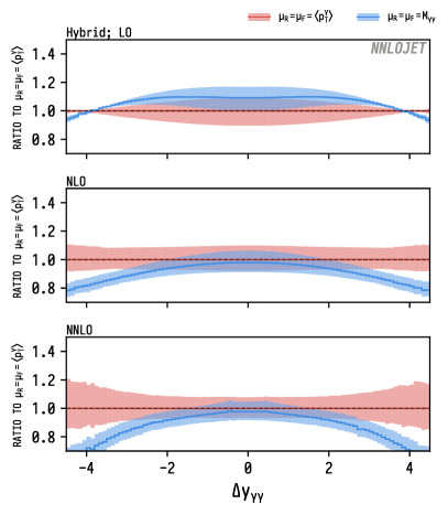
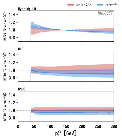
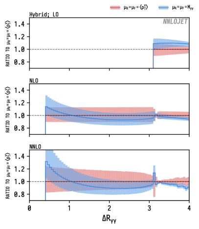
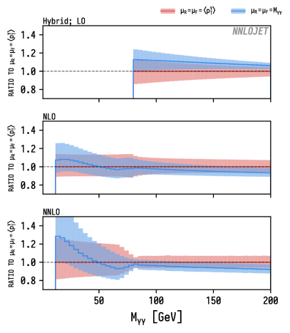
Figure 12: Order-by-order comparison of the difference between the scale choice $\mu_{0}=M_{\gamma\gamma}$ and $\mu_{0}=\left\langle p_{\mathrm{T}}^{\gamma}\right\rangle$. Leading order here means $\alpha_{\mathrm{s}}^{0}$, so the counterbalancing effects of the PDFs and the running of $\alpha_{\mathrm{s}}$ can be deduced.

3.4 Alternative scale functional forms

We remark on the elements of the above discussion which carry over to scale choices with functional forms other than $\mu_{0}=M_{\gamma\gamma}$ and $\mu_{0}=\left\langle p_{\mathrm{T}}^{\gamma}\right\rangle$. Popular candidates commonly found in studies of other processes typically involve a weighted average, mixing four-momentum-invariant-type observables with transverse-plane observables, schematically of the form

$$\mu_{0}=\left(\alpha M_{\gamma\gamma}^{r}+\beta f\left(\left\{\mathbf{p}_{\mathrm{T},{i}}\right\}\right)^{r}\right)^{\frac{1}{r}}$$ (28)

where common choices for $f$ include $p_{\mathrm{T}}^{\gamma\gamma}$, the transverse momentum of the diphoton system, or the total transverse momentum of all partons, all jets, or both photons. A variety of functional forms of this type were considered in Badger:2013ava for the production of a photon pair in association with up to three identified jets.

Functional forms containing $M_{\gamma\gamma}$, i.e. with $\alpha\neq 0$, are dominated by the exponential function of rapidity separation in the (sufficiently) large rapidity-separation region discussed above, and so behave like $M_{\gamma\gamma}$ there. The results in this region therefore lie within the envelope bounded by the scale variation $\mu\in\left\{\frac{1}{2}M_{\gamma\gamma},2M_{\gamma\gamma}\right\}$. Of particular importance is the choice

$$\mu_{0}=M_{\mathrm{T},\gamma\gamma} =\sqrt{M_{\gamma\gamma}^{2}+\left(p_{\mathrm{T}}^{\gamma\gamma}\right)^{2}}$$

$$=\sqrt{\left(p_{\mathrm{T}}^{\gamma_{1}}\right)^{2}+\left(p_{\mathrm{T}}^{\gamma_{2}}\right)^{2}+2p_{\mathrm{T}}^{\gamma_{1}}p_{\mathrm{T}}^{\gamma_{2}}\cosh\Delta y_{\gamma\gamma}}$$ (29)

which was considered in Catani:2018krb and shows identical behaviour in this limit. In addition, the scales $H^{\prime}_{\mathrm{T}},\hat{H}^{\prime}_{\mathrm{T}},\sqrt{\Sigma^{2}}$ and $\sqrt{\hat{\Sigma}^{2}}$ that were investigated for diphoton production in association with up to three jets in Badger:2013ava all have similar behaviour, as a consequence of their dependence on $M_{\gamma\gamma}$.

From a physical perspective, the behaviour in this limit represents the scale ambiguity between transverse-plane and four-momentum observables. For central final-states, both classes of observable are of the same order of magnitude and induce a similar ordering of events by scale. For events with large rapidity separation, the projection onto the transverse plane dramatically changes the apparent energy scale of the event. In the extremes of rapidity separation we enter the two-large-scales regime, in which resummation or other approaches may become relevant to correct for large logarithms of the form $\ln\left(\hat{s}/{E_{\mathrm{T}}^{{2}}}\right)$. It is possible that compensating behaviour partially accounting for these logarithms would arise in the parton distribution functions if one or the other type of scale was used consistently in fits.

The second region discussed above, of small $\Delta R_{\gamma\gamma}$, arises as a direct consequence of the specific form of the angular factor $\left(\cosh\Delta y_{\gamma\gamma}-\cos\Delta\phi_{\gamma\gamma}\right)$ in $M_{\gamma\gamma}$, which reduces to $\Delta R_{\gamma\gamma}$ in this limit. As a result, modifying $M_{\gamma\gamma}$ by any offset function $f$ with a non-zero limit as $\Delta R_{\gamma\gamma}\to 0$ rectifies the problematic behaviour. This is the case for $M_{\mathrm{T},\gamma\gamma}$ in section 3.4 above, and all other scales considered with non-zero $\beta$. Whilst candidates for $f$ with similar asymptotic behaviour to $M_{\gamma\gamma}$ do exist (e.g. $f=p_{\mathrm{T}}^{\gamma_{1}}p_{\mathrm{T}}^{\gamma_{2}}\Delta R_{\gamma\gamma}$), they do not arise naturally from a consideration of the scale of the process. From a physical perspective, problematic behaviour in this region can be explained as the failure of the scale $M_{\gamma\gamma}$ to capture the natural scale of the underlying process, in which the collimated diphoton pair recoils against a hard jet. The scale variable vanishes as the two photons become collinear, restricted only by the experimental cut, even as the event maps onto a photon-plus-jet event of characteristic scale $p_{\mathrm{T}}^{\gamma}\sim p_{\mathrm{T}}^{j}$. This leads to exaggerated contributions from $\alpha_{\mathrm{s}}$ which are not compensated by the real-virtual matrix elements.

We can understand this substantial exposure as follows. The diphoton final-state is a two-particle final-state, so the Born-level kinematics are highly restricted; it is colourless, so only the ${q}{\bar{q}}$-channel is fully NNLO, and there is no resonant propagator, so the cross-section is not dominated by a single modal value of the final-state invariant mass. It might therefore be expected that other final-states are unlikely to yield similar sensitivities. Nevertheless, with the same cuts, the same ratios of scales would arise for, e.g., the $Z\to 2\ell$ process, and it may be worth investigating their impact further.

4 Combined effect of isolation and scale variation

Finally we illustrate the combined effect of the simultaneous variation of scale and isolation choice on the distributions. We have previously seen in fig. 7 that the region of phase-space most affected by the difference between smooth-cone and hybrid isolation is that in which $\Delta R_{\gamma\gamma}$ is small, and that the same region is highly sensitive to the scale choice, growing starkly with the running coupling relative to a prediction using a scale independent of $\Delta R_{\gamma\gamma}$.

We therefore examine the relative size of these competing effects in fig. 13. In the top panel, suppression of the cross-section for smooth-cone isolation as $\Delta R_{\gamma\gamma}\to 0$ competes with the enhancement from the scale $M_{\gamma\gamma}$ to leave the ratio almost flat. As a result, for this specific combination of isolation procedure and scale choice, the competing effects of each choice shown in the lower two panels are disguised, leaving distributions that differ by an overall normalisation.

Away from this region, which is the region not populated by the Born kinematics, the ratio is stable.

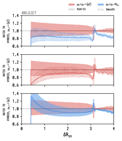
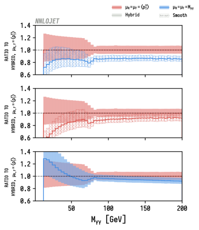
Figure 13: Combined ratio plots for four-way scales and isolation comparison, at NNLO (ratio to $\mu_{\mathrm{F}}=\mu_{\mathrm{R}}=\left\langle p_{\mathrm{T}}^{\gamma}\right\rangle$ with hybrid isolation).

4.1 Comparison to ATLAS data: four-way comparison

In this section we compare the four combinations of choices for isolation and scale to ATLAS 8 TeV data Aaboud:2017vol , with the cuts of eq. 22. As elsewhere, for both smooth-cone and (matched) hybrid isolation we use a cone of radius $0.4$ and a threshold $E_{\mathrm{T}}^{{\text{thr.}}}=11~{}\mathrm{GeV}$, whilst for matched-hybrid isolation we use inner-cone radius $R_{d}=0.1$.

We begin in fig. 14 with the two fully-NNLO distributions $\mathrm{d}\sigma/\mathrm{d}M_{\gamma\gamma}$ and $\mathrm{d}\sigma/\mathrm{d}\left|\cos{{\theta_{\eta}^{\ast}}}\right|$. The features highlighted above can now be seen to dramatically improve the overall agreement of the prediction with the data.

We consider first the $M_{\gamma\gamma}$ distribution. The first panel shows that the overall prediction for the conventional scale choice and isolation procedure, $\mu_{0}=M_{\gamma\gamma}$ with smooth-cone isolation, consistently underestimates the data by about 20%, except in the largest $M_{\gamma\gamma}$ bins. Agreement within the scale uncertainty band of the NNLO prediction occurs only at the extremes of the distribution, in the lowest and highest $M_{\gamma\gamma}$ bins.

The second panel shows that, in the low-$M_{\gamma\gamma}$ region, the agreement observed in the first panel is a direct consequence of the low-$M_{\gamma\gamma}$ enhancement for $\mu_{0}=M_{\gamma\gamma}$ outlined previously. Without it, the suppression resulting from smooth-cone isolation prevents agreement in this region. Conversely, the third panel shows that without the additional suppressive behaviour of smooth-cone isolation on the low-$M_{\gamma\gamma}$ prediction, it grows substantially relative to the data, which does not follow the same low-$M_{\gamma\gamma}$ behaviour.

Comparing the first and third panels, we see that with $\mu_{0}=M_{\gamma\gamma}$, moving from smooth-cone to hybrid isolation leads to a prediction in better agreement with the data, though still not consistently within the scale uncertainties of the theory calculation. We also see that with the scale choice $M_{\gamma\gamma}$, and without the suppression due to smooth-cone isolation, the low-$M_{\gamma\gamma}$ behaviour arising from the scale choice is untamed, and leads to a growing deviation between theory and data as $M_{\gamma\gamma}$ decreases.

The last panel shows that without either the enhancement due to $\mu_{0}=M_{\gamma\gamma}$ for small $M_{\gamma\gamma}$, or the suppression in the same region due to smooth-cone isolation for small $\Delta R_{\gamma\gamma}$, we see agreement in this region between the theory prediction and the data. The combined effects on the overall normalisation of more permissive isolation and of the alternative scale choice $\mu_{0}=\left\langle p_{\mathrm{T}}^{\gamma}\right\rangle$ correct the 20% suppression throughout the distribution, resulting in theory predictions and experimental measurements largely agreeing within the scale uncertainty bands throughout the distribution, except in the highest $M_{\gamma\gamma}$ bin where we might expect missing electroweak contributions to become significant.

We now turn to the $\left|\cos{{\theta_{\eta}^{\ast}}}\right|$ distribution, defined by

$$\left|\cos{{\theta_{\eta}^{\ast}}}\right|=\tanh{\left(\frac{1}{2}\left|\Delta\eta_{\gamma\gamma}\right|\right)}$$ (30)

which is plotted for reference in fig. 15. In the first panel in fig. 14 we see that the prediction with the scale choice $\mu_{0}=M_{\gamma\gamma}$ and smooth-cone isolation substantially undershoots the data, by 15% at small rapidity-separations and 40% at high rapidity-separations. This is absent for the scale choice $\mu_{0}=\left\langle p_{\mathrm{T}}^{\gamma}\right\rangle$ in panels 2 and 4, and is therefore an artefact arising directly from the scale $M_{\gamma\gamma}$ and its approximately-exponential growth with rapidity separation as discussed in section 3.3. Any other scale that is independent of $\Delta y_{\gamma\gamma}$ (or, in the notation of section 3.4, with $\alpha=0$) would be expected to show a similarly flat ratio to the data. Clearly, for fixed-order predictions made with $\mu_{0}=M_{\gamma\gamma}$ to exhibit such a ratio, the PDFs would need to grow to counterbalance the suppression of the cross-section. It is not clear that this would be possible in such a way as to allow simultaneous agreement with data with both categories of scales.

As expected, between panels 1 and 3, and 2 and 4, the change in isolation between smooth-cone and hybrid-isolation yields an flat upwards normalisation, resulting in very good agreement across the rapidity range for the combination $\mu_{0}=\left\langle p_{\mathrm{T}}^{\gamma}\right\rangle$ and hybrid isolation.

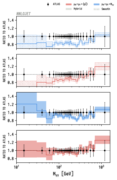
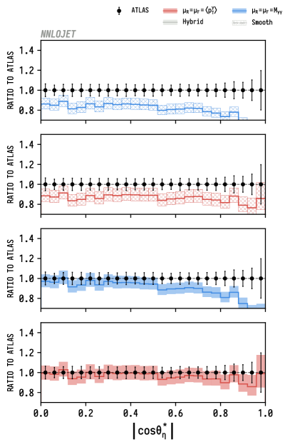
Figure 14: Combined ratio plots for the four-way scales and isolation comparison, at NNLO (ratio to data).

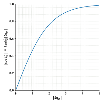
Figure 15: Relationship between $\left|\cos{{\theta_{\eta}^{\ast}}}\right|$ and $\Delta\eta_{\gamma\gamma}$. The dashed grey lines indicate the relationship between ATLAS bins for $\left|\cos{{\theta_{\eta}^{\ast}}}\right|$ and the corresponding intervals for $\Delta\eta_{\gamma\gamma}$. At ATLAS, the experimental cuts $\left|y^{\gamma}\right|<2.37$ restrict the rapidity separation to $\left|\Delta\eta_{\gamma\gamma}\right|<4.74$. This cut only affects the result the in final bin, which otherwise extends to infinite rapidity separations.

4.2 Comparison to ATLAS data: two-way comparison

We have up to now separately investigated the effect of altering scale and isolation independently. Here we examine the combined effect on the agreement with ATLAS data of the simultaneous transition between the combinations corresponding to panels 1 and 4 of the plots in fig. 14, namely

• $\mu_{0}=M_{\gamma\gamma}$ with smooth-cone isolation, and

• $\mu_{0}=\left\langle p_{\mathrm{T}}^{\gamma}\right\rangle$ with hybrid isolation.

These are plotted for the six observables which ATLAS measured in fig. 16, with axis limits and layout set to enable easy comparison with the corresponding figure (fig. 5) in the ATLAS experimental paper Aaboud:2017vol .

Across all six distributions, combination (b) gives better agreement with data almost everywhere. The regions where agreement is notably worse are those in the neighbourhood of the Sudakov singularities described in section 2.2, and hence where poor agreement is expected in the absence of resummation. In these effectively-NLO distributions we continue to see an incomplete description of the data. We can infer from the Sherpa results of Aaboud:2017vol that the missing radiative corrections that would feature in an NNLO diphoton-plus-jets calculation are required to adequately describe the data in these distributions.

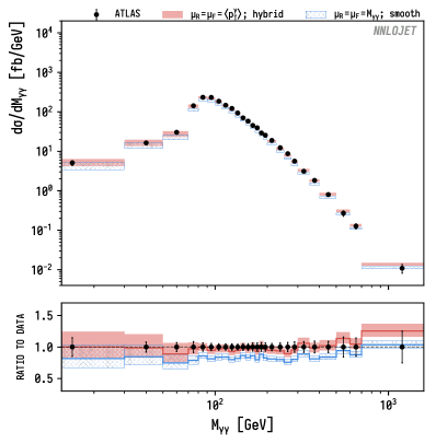
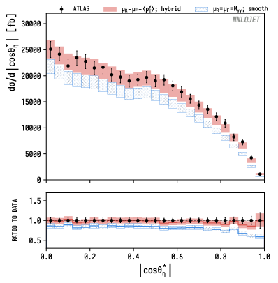
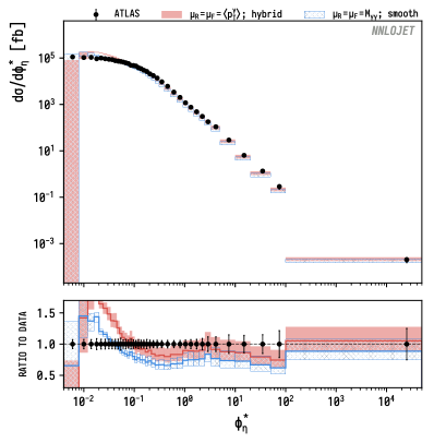
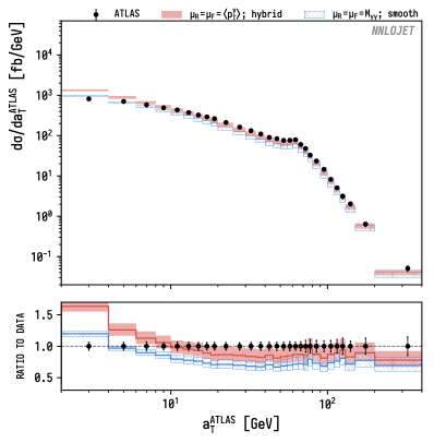
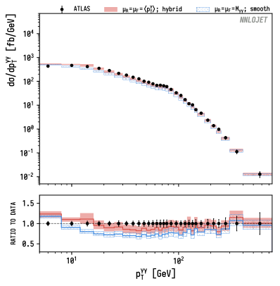
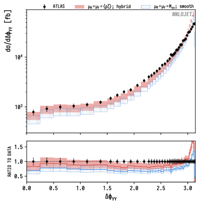
Figure 16: Re-evaluation of Figure 5 from Aaboud:2017vol showing the effects of the modified scale choice and isolation criteria on the prediction.

For completeness, in fig. 17 we show the order-by-order breakdown of the NNLO calculation for choice (b) of scale and isolation criterion, showing the relative magnitude of the NNLO corrections with these parameters.

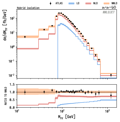
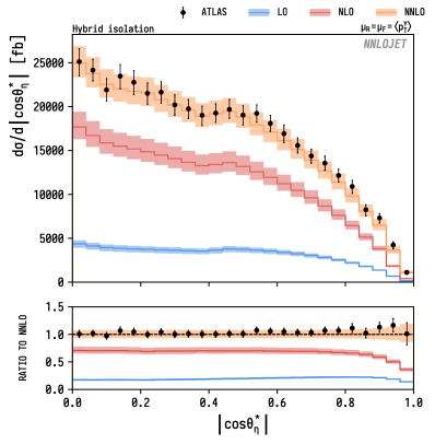
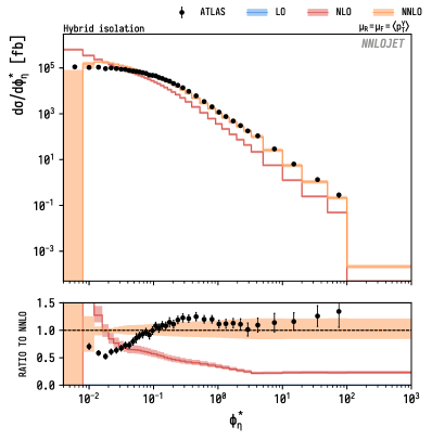
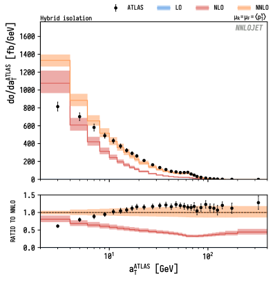
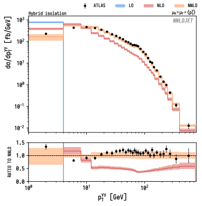
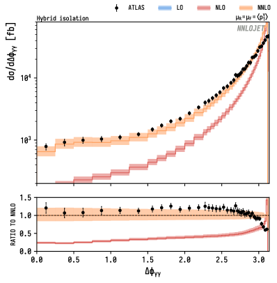
Figure 17: Illustration of the perturbative convergence of the fixed-order predictions, for the six measured ATLAS distributions.

5 Conclusions

Photon isolation is a substantial source of uncertainty in precision calculations, whose subtleties have not yet been fully explored. These uncertainties will only become more significant for phenomenology as the target precision of experiment and theory narrows. Whilst they can be mitigated through the careful choice of alternative isolation parameters, such as smaller isolation cones, it is important to understand the full effect of approximations made in the theoretical modelling of experimental isolation.

We have shown that better approximating the fiducial region defined by the experimental isolation criterion, using so-called hybrid isolation, leads to substantially improved agreement with data than the presently-favoured smooth-cone isolation. Comparing the two, smooth-cone isolation results in a suppression of the cross-section that is consistently of the order of 10%, and in regions of some distributions up to 50%.

This has re-exposed the issue of the infrared sensitivity of isolated photon differential cross-sections to fixed-cone isolation cuts. Although this was first discussed in the context of fragmentation cross-sections at NLO Binoth:1999qq , it has been absent from more recent discussions of fixed-cone and hybrid isolation. We have found that, as might be expected from the step-function formulation of all cone-based isolation criteria, discontinuities and resulting Sudakov singularities arise in all of them, but are most significant for the $\mathrm{d}\sigma/\mathrm{d}p_{\mathrm{T}}^{\gamma\gamma}$ distribution for fixed-cone isolation with a constant threshold. These pathological regions are not currently of direct phenomenological significance, but may become so in future. Indirectly, they are likely to have implications for phenomenology by hindering cut-based subtraction procedures for higher-order perturbative calculations.

We have likewise studied the uncertainty resulting from the choice of functional form for the dynamic renormalisation and factorisation scales. As for the profile-function-induced uncertainty, we have found that the envelope of predictions spanned by different reasonable choices of functional form is not adequately described by the usual scale variation procedure of varying a central scale up and down by combinations of factors of 2 in each direction. We have identified the regions of phase-space in which two reasonable choices are most likely to give very different results, and verified that the sensitivity in these regions is indeed substantial.

We have identified competing effects arising from the conventional choices of the two theoretical functions described above, each of which disguises the effect of the other on the result. We have shown that these choices, of smooth-cone isolation and $\mu_{0}=M_{\gamma\gamma}$, are interdependent, in that unphysical behaviour introduced by the choice of smooth-cone isolation is only absent from the result with the scale choice $\mu_{0}=M_{\gamma\gamma}$, and vice versa.

Comparing the above findings to ATLAS 8 TeV data, we conclude that these two effects account both for the deviation of the central NNLO predictions from the experimental data, and for the underestimation of the theoretical uncertainty that places the experimental result outside of the theoretical uncertainty bands. Without properly accounting for this uncertainty, the natural conclusion is that the experimental measurements disagree with the theoretical predictions at NNLO. In fact, reasonable choices for scale setting and isolation procedures give excellent agreement. Further measurements of other genuine NNLO distributions will be required to test whether this agreement persists at higher centre-of-mass energies and in other NNLO distributions.

References

- (1) ATLAS collaboration, Measurements of Higgs boson properties in the diphoton decay channel with 36 fb-1 of collision data at TeV with the ATLAS detector, Phys. Rev. D 98 (2018) 052005 [1802.04146].
- (2) CMS collaboration, A measurement of the Higgs boson mass in the diphoton decay channel, Phys. Lett. B 805 (2020) 135425 [2002.06398].
- (3) ATLAS collaboration, Search for new phenomena in high-mass diphoton final states using 37 fb-1 of proton–proton collisions collected at TeV with the ATLAS detector, Phys. Lett. B 775 (2017) 105 [1707.04147].
- (4) CMS collaboration, Search for physics beyond the standard model in high-mass diphoton events from proton-proton collisions at 13 TeV, Phys. Rev. D 98 (2018) 092001 [1809.00327].
- (5) S. Frixione, Isolated photons in perturbative QCD, Phys. Lett. B 429 (1998) 369 [hep-ph/9801442].
- (6) OPAL collaboration, Measurement of isolated prompt photon production in photon photon collisions at GeV, Eur. Phys. J. C 31 (2003) 491 [hep-ex/0305075].
- (7) SM, NLO Multileg Working Group collaboration, The SM and NLO Multileg Working Group: Summary report, in 6th Les Houches Workshop on Physics at TeV Colliders, pp. 21–189, Mar., 2010 [1003.1241].
- (8) Z. Hall and J. Thaler, Photon isolation and jet substructure, JHEP 09 (2018) 164 [1805.11622].
- (9) E.W.N. Glover and A. Morgan, Measuring the photon fragmentation function at LEP, Z. Phys. C 62 (1994) 311.
- (10) S. Catani, L. Cieri, D. de Florian, G. Ferrera and M. Grazzini, Diphoton production at hadron colliders: a fully-differential QCD calculation at NNLO, Phys. Rev. Lett. 108 (2012) 072001 [1110.2375].
- (11) J.M. Campbell, R. Ellis, Y. Li and C. Williams, Predictions for diphoton production at the LHC through NNLO in QCD, JHEP 07 (2016) 148 [1603.02663].
- (12) H.A. Chawdhry, M.L. Czakon, A. Mitov and R. Poncelet, NNLO QCD corrections to three-photon production at the LHC, JHEP 02 (2020) 057 [1911.00479].
- (13) F. Siegert, A practical guide to event generation for prompt photon production with Sherpa, J. Phys. G 44 (2017) 044007 [1611.07226].
- (14) S. Amoroso et al., Les Houches 2019: Physics at TeV Colliders: Standard Model Working Group Report, in 11th Les Houches Workshop on Physics at TeV Colliders: PhysTeV Les Houches, Mar., 2020 [2003.01700].
- (15) M.A. Ebert and F.J. Tackmann, Impact of isolation and fiducial cuts on qT and N-jettiness subtractions, JHEP 03 (2020) 158 [1911.08486].
- (16) S. Catani, L. Cieri, D. de Florian, G. Ferrera and M. Grazzini, Diphoton production at the LHC: a QCD study up to NNLO, JHEP 04 (2018) 142 [1802.02095].
- (17) ATLAS collaboration, Measurements of integrated and differential cross sections for isolated photon pair production in collisions at TeV with the ATLAS detector, Phys. Rev. D 95 (2017) 112005 [1704.03839].
- (18) S. Catani, M. Fontannaz, J. Guillet and E. Pilon, Isolating Prompt Photons with Narrow Cones, JHEP 09 (2013) 007 [1306.6498].
- (19) S. Catani, M. Fontannaz, J. Guillet and E. Pilon, Cross-section of isolated prompt photons in hadron hadron collisions, JHEP 05 (2002) 028 [hep-ph/0204023].
- (20) T. Binoth, J. Guillet, E. Pilon and M. Werlen, A Full next-to-leading order study of direct photon pair production in hadronic collisions, Eur. Phys. J. C 16 (2000) 311 [hep-ph/9911340].
- (21) S. Frixione and G. Ridolfi, Jet photoproduction at HERA, Nucl. Phys. B 507 (1997) 315 [hep-ph/9707345].
- (22) S. Catani and B. Webber, Infrared safe but infinite: Soft gluon divergences inside the physical region, JHEP 10 (1997) 005 [hep-ph/9710333].
- (23) M. Grazzini, S. Kallweit and M. Wiesemann, Fully differential NNLO computations with MATRIX, Eur. Phys. J. C 78 (2018) 537 [1711.06631].
- (24) NNPDF collaboration, Parton distributions from high-precision collider data, Eur. Phys. J. C 77 (2017) 663 [1706.00428].
- (25) T. Binoth, J. Guillet, E. Pilon and M. Werlen, Beyond leading order effects in photon pair production at the Tevatron, Phys. Rev. D 63 (2001) 114016 [hep-ph/0012191].
- (26) CDF collaboration, Measurement of the Cross Section for Prompt Isolated Diphoton Production Using the Full CDF Run II Data Sample, Phys. Rev. Lett. 110 (2013) 101801 [1212.4204].
- (27) D0 collaboration, Measurement of the differential cross sections for isolated direct photon pair production in collisions at TeV, Phys. Lett. B 725 (2013) 6 [1301.4536].
- (28) CMS collaboration, Measurement of differential cross sections for the production of a pair of isolated photons in pp collisions at , Eur. Phys. J. C 74 (2014) 3129 [1405.7225].
- (29) ATLAS collaboration, Measurement of isolated-photon pair production in collisions at TeV with the ATLAS detector, JHEP 01 (2013) 086 [1211.1913].
- (30) J.M. Campbell, R.K. Ellis and C. Williams, Direct Photon Production at Next-to–Next-to-Leading Order, Phys. Rev. Lett. 118 (2017) 222001 [1612.04333].
- (31) X. Chen, T. Gehrmann, E.W.N. Glover, M. Höfer and A. Huss, Isolated photon and photon+jet production at NNLO QCD accuracy, JHEP 04 (2020) 166 [1904.01044].
- (32) J.M. Campbell, J. Rojo, E. Slade and C. Williams, Direct photon production and PDF fits reloaded, Eur. Phys. J. C 78 (2018) 470 [1802.03021].
- (33) J.M. Campbell and C. Williams, Triphoton production at hadron colliders, Phys. Rev. D 89 (2014) 113001 [1403.2641].
- (34) R. Abdul Khalek et al., Phenomenology of NNLO jet production at the LHC and its impact on parton distributions, Eur. Phys. J. C 80 (2020) 797 [2005.11327].
- (35) S. Badger, A. Guffanti and V. Yundin, Next-to-leading order QCD corrections to di-photon production in association with up to three jets at the Large Hadron Collider, JHEP 03 (2014) 122 [1312.5927].