The Ecological Impact of High-performance Computing in Astrophysics

Abstract

The importance of computing in astronomy continues to increase, and so is its impact on the environment. When analyzing data or performing simulations, most researchers raise concerns about the time to reach a solution rather than its impact on the environment. Luckily, a reduced time-to-solution due to faster hardware or optimizations in the software generally also leads to a smaller carbon footprint. This is not the case when the reduced wall-clock time is achieved by overclocking the processor, or when using supercomputers.

The increase in the popularity of interpreted scripting languages, and the general availability of high-performance workstations form a considerable threat to the environment. A similar concern can be raised about the trend of running single-core instead of adopting efficient many-core programming paradigms.

In astronomy, computing is among the top producers of green-house gasses, surpassing telescope operations. Here I hope to raise the awareness of the environmental impact of running non-optimized code on overpowered computer hardware.

Leiden Observatory, Leiden University, PO Box 9513, 2300 RA, Leiden, The Netherlands

1 Carbon footprint of computing

The fourth pillar of science, simulation and modeling, already had a solid foothold in 4th-century astronomy [1, 2], but this discipline flourished with the introduction of digital computers. One of its challenges is the carbon emission caused by this increased popularity. Unrecognized as of yet by UNESCO [EOLSS2020] the carbon footprint of computing in astrophysics should be emphasized. One purpose of this document is to raise this awareness.

In figure 1, we compare the average Human production of CO₂ (red lines) with other activities, such as telescope operation, the emission of an average astronomer [3] and finishing a (four year) PhD [4].

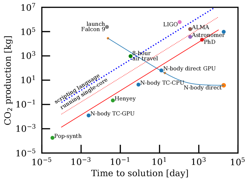
Figure 1: CO² emission (in kg) as a function of the time to solution (in days) for a variety of popular computational techniques employed in astrophysics, and other activities common among astronomers [4, 3]. The solid red curve gives the current individual world-average production, whereas the dotted curves give the maximum country average. The LIGO carbon production is taken over its first 106-day run (using $\sim 180$ kW) [5], and for ALMA a 1-year average [6]. A Falcon 9 launch lasts about 32 minutes during which $\sim 110\,000$ liters of highly refined kerosene is burned. The tree-code running on GPU is performed using $N=2^{20}$ particles. The direct N-body code on CPU (right-most blue bullet) was run with $N=2^{13}$ [7], and the other codes with $N=2^{16}$. All performance results were scaled to $N=2^{20}$ particles. The calculations were performed for 10 N-body time units [8]. The energy consumption was computed using the scaling relations of [9] and a conversion of KWh to Co₂ of $0.283$ kWh/kg. The blue dotted curve shows the estimated carbon emission when these calculations would have been implemented in Python running on a single core. The solid blue curve to the right, starting with the orange bullet shows how the performance and carbon production changes while increasing the number of compute cores from 1 to $10^{6}$ (out of a total of $7\,299\,072$, left-most orange point) using the performance model by [10].

While large observing facilities cut down on carbon footprint by offering remote operation, the increased speed of computing resources can hardly be compensated by their increased efficiency. This also is demonstrated in figure 1, where we compare measurements for several popular computing activities. These measurements are generated using the Astrophysical Multiuser Software Environment [11], in which the vast majority of the work is done in optimized and compiled code.

We include simulations of the Sun’s evolution from birth to the asymptotic giant branch using a Henyey solver [12] and parametrized population-synthesis [13] (green bullets).

We also present timings for simulating the evolution of a self-gravitating system of a million equal-mass point-particles in a virialized Plummer sphere for 10 dynamical time-scales. These calculations are performed by direct integration (with the 4th-order Hermite algorithm) and using a hierarchical tree-code (with leapfrog algorithm). Both calculations are performed on CPU as well as with graphics processing unit (GPU). Not surprisingly, the tree-code running single GPU is about a million times faster than the direct-force calculations on CPU; One factor $1000$ originates from the many-cores of the GPU [14], and the other from the favorite scaling of the tree algorithm [15]. The trend in carbon production is also not surprising; shorter runtime leads to less carbon. The emission of carbon while running a workstation is comparable to the world’s per-capita average.

Now consider single-core versus multi-core performance of the direct $N$-body code in figure 1. The blue bullet to the right gives the single-core workstation performance, but the large orange bullet below it shows the single-core performance on today’s largest supercomputer [16]. The blue curve gives the multi-core scaling up to $10^{6}$ cores (left-most orange point). The relation between the time-to-solution and the carbon footprint of the calculations is not linear. When running a single core, the supercomputer produces less carbon than a workstation (we assumed the supercomputer to be used to capacity by other users). Adopting more cores result in better performance, at the cost of producing more carbon. Similar performance as a single GPU is reached when running $1000$ cores, but when the number of cores is further increased, the performance continues to grow at an enormous cost in carbon production. When running a million cores, the emission of running a supercomputer by far exceeds air travel and approaches the carbon footprint of launching a rocket into space.

2 Concurrency for lower emission

When parallelism is optimally utilized, the highest performance is reached for the maximum core count, but the optimal combination of performance and carbon emission is reached for $\sim 1000$ cores, after which the supercomputer starts to produce more carbon than a workstation. The improved energy characteristics for parallel operation and its eventual decline is further illustrated in the Z-plot presented in figure 2, showing energy consumption as a function of the performance of 96 cores (192 hyperthreaded) workstation.

Running single core on a workstation is inefficiently slow and produces more carbon than running multi-core. Performance continues to increase with core count, but optimal energy consumption is reached when running 64 and 96 physical cores (green star in figure 2). Running more cores will continue to reduce the time-to-solution, but at higher emission. Note that the carbon emission of the parallel calculation (blue curve in figure 1) does not drop, because we assumed that the supercomputer is optimally shared, whereas we assumed that the workstation used in the Z-plot figure was private.

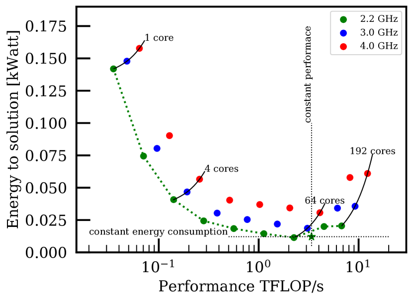
Figure 2: Energy to solution as a function of code performance. The Z-plot gives for a number of processor (and processor frequencies) and the energy consumed (in kWatt) as a function of performance (in TFLOP/s) [9]. The runs (green dots) were performed using a quad CPU 24-core (48 hyperthreaded) Intel Xeon E7-8890 v4 at 2.20 GHz calculated with 1, 2, 4, …, 192 cores. Curves of constant core-count are indicated for 1, 4, 64 and 192 cores (solid curves). The other colored points (blue and red) give the relation for overclocking the processor to 3 and 4 GHz, scaled from the measured points using over-clocking emission relations [17]. Dotted curves give constant energy-requirement-to-solution (horizontal) and sustained processor performance (vertical). The star at the cross of these two curves is measured using 96 cores. The calculations are performed Bulirsch-Stoer algorithm with a Leofrog integration [18] at a tolerance of $\log(dE/E)=-8$ using a wordlength of 64 bits.

When scaling our measurements of the compute performance and energy consumption with the clock frequency of the processor (blue and red points for each core-count) reduces wall-clock time, but costs considerably more energy (see also [19]). Although not shown here, reducing clock-speed slows down the computer while increasing the energy requirement.

If the climate is a concern, prevent occupying a supercomputer to capacity. The wish for more environmentally friendly supercomputers triggered the contest for the greenest supercomputers [20]. Since the inauguration of the green500, the performance per Watt has increased from 0.23 Tflop/kW by a Blue Gene/L in 2007 [20] to more than 20 Tflop/kW by the MN-3 core-server today [16]. This enormous increase in performance per Watt is mediated by the further development of low-power many-core architectures, such as the GPU. The efficiency of modern workstations, however, has been lagging. A single core of the Intel Xeon E7-8890, for example runs at $\sim 4$ TFLOP/kWatt, and the popular Intel core-i7 920 tops only 0.43 TFLOP/kWatt. Workstation processors have not kept up with the improved carbon characteristics of GPUs and supercomputers.

For optimal operation, run few ($\sim 1000$) cores on a supercomputer or a GPU-equipped workstation. When running a workstation, use as many physical cores as possible, but leave the virtual cores alone. Over-clocking reduces wall-clock time but at a greater environmental impact.

3 The role of language on the ecology

So far, we assumed that astrophysicists invest in full code optimization that uses the hardware optimally. However, in practice, most effort is generally invested in developing the research question, after which designing, writing, and running the code is not the primary concern. This holds so long as the code-writing and execution are sufficiently fast. As a consequence, relatively inefficient interpreted scripting languages, such as Python, rapidly grow in popularity.

According to the Astronomical Source Code Library (ASCL [21]), $\sim 43$% of the code is written in Python, and 7 % Java, IDL and Mathematica. Only 18%, 17% and 16% of codes are written in Fortran, C and C++ respectively. Python is popular because it is interactive, strongly and dynamically typed, modular, object-oriented, and portable. But most of all, Python is easy to learn and it gets the job done without much effort, whereas writing in C++ or Fortran can be rather elaborate. The expressiveness of Python considerably outranks the Fortran and C families of programming languages.

The main disadvantage of Python, however, is its relatively slow speed compared to compiled languages. In figure 3, we present an estimate of the amount of CO₂ produced when performing a direct N-body calculation of $2^{14}$ equal-mass particles in a virialized Plummer sphere. Each calculation was performed for the same amount of time and scaled to 1 day for the implementation in C++.

Python (and to a lesser extend Java) take considerably more time to run and produce more CO₂ than C++ or Fortran. Python and Java are also less efficient in terms of energy per operation than compiled languages [22], which explains the offset away from the dotted curve.

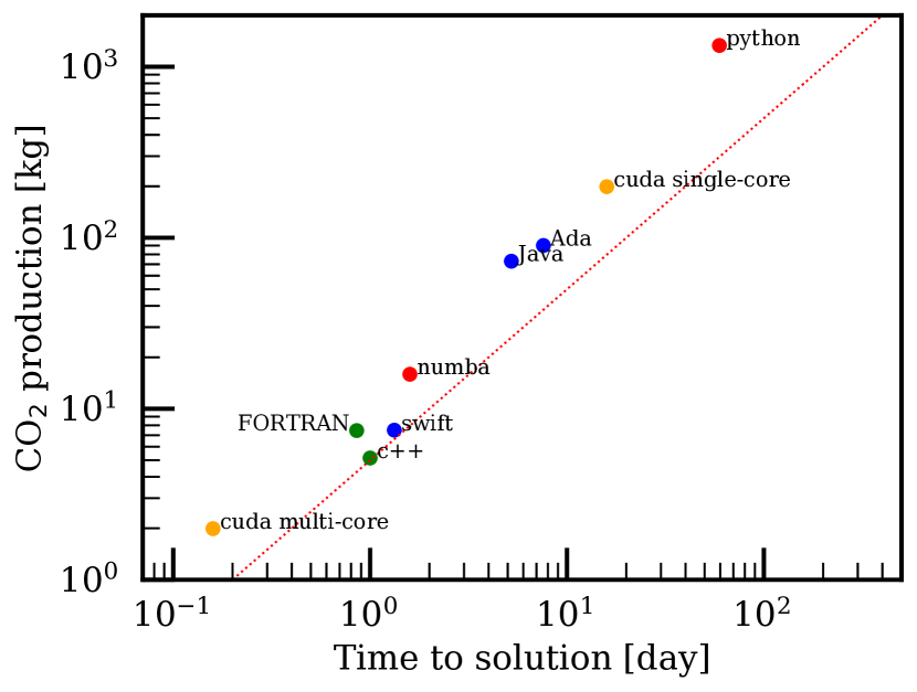
Figure 3: Here we used the direct $N$-body code from [23] to measure execution speed and the relative energy efficiency for each programming language from table 3  of [22]. The dotted red curve gives a linear relation between the time-to-solution and carbon footprint ($\sim 5$ kg CO₂/day). The calculations were performed on a 2.7GHz Intel Xeon E-2176M CPU and NVIDIA Tesla P100 GPU.

The growing popularity of Python is disquieting. Among 27 tested languages, only Perl and Lua are slower [22]. The runtime performance of Python can be improved in a myriad of ways. Most popular are the numba or NumPy libraries, which offer pre-compiled code for common operations. In principle, numba and NumPy can lead to an enormous increase in speed and reduced carbon emission. However, these libraries are rarely adopted for reducing carbon emission or runtime with more than an order of magnitude [21]. NumPy, for example, is mostly used for its advanced array handling and support functions. Using these will reduce runtime and, therefore, also carbon emission, but optimization is generally stopped as soon as the calculation runs within an unconsciously determined reasonable amount of time, such as the coffee-refill time-scale or a holiday weekend.

In figure 1 we presented an estimate of the carbon emission as a function of runtime for Python implementations (see blue dotted curve) of popular applications (green and blue bullets). The continuing popularity of Python should be confronted with the ecological consequences. We even teach Python to students, but also researchers accept the performance punch without realizing the ecological impact. Using C++ and Fortran instead of Python would save enormously in terms of runtime and CO₂ production. Implementing in CUDA and run on a GPU would even be better for the environment, but the authors know from first-hand experience that this poses other challenges, and that it takes years of research [7], before a tuned instrument is production-ready [24].

4 Conclusions

The popularity of computing in research is proliferating. This impacts the environment by increased carbon emission.

The availability of powerful workstations and running Python scripts on single cores is about the worst one can do for the environment. Still, this mode of operation seems to be most popular among astronomers. This trend is stimulated by the educational system and mediated by Python’s rapid prototyping-abilities and the ready availability of desktop workstations. This trend leads to an unnecessarily large carbon footprint for computationally-oriented astrophysical research. The importance of rapid prototyping appears to outweigh the ecological impact of inefficient code.

The carbon footprint of computational astrophysics can be reduced substantially by running on GPUs. The development time of such code, however, requires major investments in time and requires considerable expertise. As an alternative, one could run concurrently using multiple the cores, rather than a single thread. It is even better to port the code to a supercomputer and share the resources. Best however, for the environment is to abandon Python for a more environmentally friendly (compiled) programming language. This would improve runtime and reduces CO₂ emission.

There are several excellent alternatives to Python. The first choice is to utilize high-performance libraries, such as NumPy and Numba. But there are other interesting strongly-typed languages with characteristics similar to Python, such as Alice, Julia, Rust, and Swift. These languages offer the flexibility of Python but with the performance of compiled C++. Educators may want to reconsider teaching Python to University students. There are plenty environmentally friendly alternatives.

While being aware of the ecological impact of high-performance computing, maybe we should be more reluctant in performing specific calculations, and consider the environmental consequences before performing a simulation. What responsibility do scientists have in assuring that their computing environment is mostly harmless to the environment?

Acknoweldgments

It is a pleasure to thank Alice Allen discussions.

We used the Python [25], matplotlib [26], numpy [27], and AMUSE [11] open source packages. Calculations ware performed using the LGM-II (NWO grant # 621.016.701), TITAN (LANL), and ALICE (Leiden University).

References

- [1] M. Ossendrijver, “Ancient Babylonian astronomers calculated Jupiter’s position from the area under a time-velocity graph,” Science, vol. 351, pp. 482–484, Jan. 2016.
- [2] T. Freeth, Y. Bitsakis, X. Moussas, J. H. Seiradakis, A. Tselikas, H. Mangou, M. Zafeiropoulou, R. Hadland, D. Bate, A. Ramsey, M. Allen, A. Crawley, P. Hockley, T. Malzbender, D. Gelb, W. Ambrisco, and M. G. Edmunds, “Decoding the ancient Greek astronomical calculator known as the Antikythera Mechanism,” Nat , vol. 444, no. 7119, pp. 587–591, Nov. 2006.
- [3] A. R. H. Stevens, S. Bellstedt, P. J. Elahi, and M. T. Murphy, “The imperative to reduce carbon emissions in astronomy,” arXiv e-prints, p. arXiv:1912.05834, Dec. 2019.
- [4] W. M. Achten, J. Almeida, and B. Muys, “Carbon footprint of science: More than flying,” Ecological Indicators, vol. 34, pp. 352 – 355, 2013. [Online]. Available: http://www.sciencedirect.com/science/article/pii/S1470160X13002306
- [5] L. S. Collaboration, “Advanced ligo reference document: Ligo m060056-v2,” 22 March 2011. [Online]. Available: https://dcc.ligo.org/public/0001/M060056/002/
- [6] L. D’Addario, “Digital Signal Processing for Large Radio Telescopes: The Challenge of Power Consumption and How To Solve It,” in Exascale Radio Astronomy, vol. 2, Apr. 2014, p. 30201.
- [7] S. F. Portegies Zwart, R. G. Belleman, and P. M. Geldof, “High-performance direct gravitational N-body simulations on graphics processing units,” New Astronomy, vol. 12, pp. 641–650, Nov. 2007.
- [8] D. C. Heggie and R. D. Mathieu, “Standardised Units and Time Scales,” in The Use of Supercomputers in Stellar Dynamics, ser. Lecture Notes in Physics, Berlin Springer Verlag, P. Hut and S. L. W. McMillan, Eds., vol. 267, 1986, p. 233.
- [9] M. Wittmann, G. Hager, T. Zeiser, and G. Wellein, “An analysis of energy-optimized lattice-boltzmann CFD simulations from the chip to the highly parallel level,” CoRR, vol. abs/1304.7664, 2013. [Online]. Available: http://arxiv.org/abs/1304.7664
- [10] F. C. Heinrich, T. Cornebize, A. Degomme, A. Legrand, A. Carpen-Amarie, S. Hunold, A.-C. Orgerie, and M. Quinson, “Predicting the Energy Consumption of MPI Applications at Scale Using a Single Node,” in Cluster 2017. Hawaii, United States: IEEE, Sep. 2017. [Online]. Available: https://hal.inria.fr/hal-01523608
- [11] S. Portegies Zwart and S. McMillan, Astrophysical Recipes; The art of AMUSE, 2018.
- [12] B. Paxton, L. Bildsten, A. Dotter, F. Herwig, P. Lesaffre, and F. Timmes, “Modules for Experiments in Stellar Astrophysics (MESA),” ApJS , vol. 192, p. 3, Jan. 2011.
- [13] S. F. Portegies Zwart and F. Verbunt, “Population synthesis of high-mass binaries.” A&A , vol. 309, pp. 179–196, May 1996.
- [14] E. Gaburov, J. Bédorf, and S. Portegies Zwart, “Gravitational tree-code on graphics processing units: implementation in CUDA,” Procedia Computer Science, volume 1, p. 1119-1127, vol. 1, pp. 1119–1127, May 2010.
- [15] J. Barnes and P. Hut, “A Hierarchical O(NlogN) Force-Calculation Algorithm,” Nat , vol. 324, pp. 446–449, Dec. 1986.
- [16] Green500-list, “Green500-list,” 2013.
- [17] I. Cutress, “The intel xeon w-3175x review: 28 unlocked cores,” ”January 30, 2019”. [Online]. Available: https://www.anandtech.com/show/13748/the-intel-xeon-w-3175x-review-28-unlocked-cores-2999-usd
- [18] S. Portegies Zwart and T. Boekholt, “On the minimal accuracy required for simulating self-gravitating systems by means of direct n-body methods,” The Astrophysical Journal Letters, vol. 785, no. 1, pp. L3–7, 2014. [Online]. Available: http://stacks.iop.org/2041-8205/785/i=1/a=L3
- [19] J. Hofmann, G. Hager, and D. Fey, “On the accuracy and usefulness of analytic energy models for contemporary multicore processors,” CoRR, vol. abs/1803.01618, 2018. [Online]. Available: http://arxiv.org/abs/1803.01618
- [20] W. Feng and K. Cameron, “The green500 list: Encouraging sustainable supercomputing,” Computer, vol. 40, no. 12, pp. 50–55, 2007.
- [21] A. Allen, “Astronomical source code librady,” Oct. 2018. [Online]. Available: https://ascl.net/1906.011
- [22] R. Pereira, M. Couto, F. Ribeiro, R. Rua, J. Cunha, J. a. P. Fernandes, and J. a. Saraiva, “Energy efficiency across programming languages: How do energy, time, and memory relate?” in Proceedings of the 10th ACM SIGPLAN International Conference on Software Language Engineering, ser. SLE 2017. New York, NY, USA: Association for Computing Machinery, 2017, p. 256–267. [Online]. Available: https://doi.org/10.1145/3136014.3136031
- [23] S. Portegies Zwart and J. Bédorf, “Nbabel,” 2020. [Online]. Available: https://www.NBabel.org/
- [24] J. Bédorf, E. Gaburov, M. S. Fujii, K. Nitadori, T. Ishiyama, and S. Portegies Zwart, “24.77 pflops on a gravitational tree-code to simulate the milky way galaxy with 18600 gpus,” in Proceedings of the International Conference for High Performance Computing, Networking, Storage and Analysis, ser. SC ’14. Piscataway, NJ, USA: IEEE Press, 2014, pp. 54–65. [Online]. Available: http://dx.doi.org/10.1109/SC.2014.10
- [25] G. van Rossum, “Extending and embedding the Python interpreter,” Report CS-R9527, Apr. 1995.
- [26] J. D. Hunter, “Matplotlib: A 2D Graphics Environment,” Computing in Science and Engineering, vol. 9, pp. 90–95, May 2007.
- [27] T. E. Oliphant, A guide to NumPy. Trelgol Publishing USA, 2006, vol. 1.