Biorthogonal quantum criticality in non-Hermitian many-body systems

Abstract

We develop the perturbation theory of the fidelity susceptibility in biorthogonal bases for arbitrary interacting non-Hermitian many-body systems with real eigenvalues. The quantum criticality in the non-Hermitian transverse field Ising chain is investigated by the second derivative of ground-state energy and the ground-state fidelity susceptibility. We show that the system undergoes a second-order phase transition with the Ising universal class by numerically computing the critical points and the critical exponents from the finite-size scaling theory. Interestingly, our results indicate that the biorthogonal quantum phase transitions are described by the biorthogonal fidelity susceptibility instead of the conventional fidelity susceptibility.

I Introduction

The study of quantum matters and quantum phase transitions is one of the central parts in condensed matter physics Sachdev (1999). For conventional Hermitian many-body systems, a quantum phase transition is usually characterized by a qualitative change in the ground-state eigenfunction and the non-analyticity of the ground-state energy at the critical point in thermodynamic limit Sachdev (1999). The corresponding quantum state of matter can be distinguished by the order parameters or the topological quantities Levin and Wen (2006). Moreover, the nature of phase transitions (or the critical exponents) can be described and obtained by the finite-size scaling theory Fisher and Barber (1972); Fisher (1974).

Non-Hermitian systems that can be realized by a gain and loss process or by a nonreciprocal hopping exhibit many intriguing unique phenomena beyond Hermitian systems Bergholtz et al. (2021); Ashida et al. (2020), for example, the breakdown of the bulk-boundary correspondence and the non-Hermitian skin effect Lee (2016); Yao and Wang (2018); Kunst et al. (2018); Xiong (2018); Gong et al. (2018); Martinez Alvarez et al. (2018); Yokomizo and Murakami (2019); Okuma et al. (2020); Zhang et al. (2020a); Yang et al. (2020a); Wang et al. (2020); Jiang et al. (2020); Weidemann et al. (2020); Xiao et al. (2020); Borgnia et al. (2020), exceptional points and bulk Fermi arcs Heiss (2012); Kozii and Fu (2017); Hodaei et al. (2017); Zhou et al. (2018); Miri and Alu (2019); Park et al. (2019); Yang and Hu (2019); Özdemir et al. (2019); Dóra et al. (2019); Zhang et al. (2019); Jin et al. (2020); Xiao et al. (2021), phase transitions without gap closing Matsumoto et al. (2020); Yang et al. (2020b), etc. New theories or concepts, i. e. non-Bloch band theory Yao and Wang (2018); Yokomizo and Murakami (2019); Zhang et al. (2020a), usually are in demand to understand such non-Hermitian phenomena. Recently, non-Hermitian many-body physics were explored to consider the interplay of the interaction and the non-Hermiticity Jin and Song (2013); Matsumoto et al. (2020); Yang et al. (2020b); Ashida et al. (2017); Herviou et al. (2019); Chang et al. (2020); Mu et al. (2020); Lee et al. (2020); Pan et al. (2020a, b); Xu and Chen (2020); Zhang et al. (2020b); Lee (2020); Shackleton and Scheurer (2020); Liu et al. (2020); Yang et al. (2021); Hanai et al. (2019); Hamazaki et al. (2019); Xi et al. (2021); Yamamoto et al. (2019); Hanai and Littlewood (2020). One central issue is to understand the phase transition and the quantum criticality Yao and Wang (2018); Ashida et al. (2017); Dóra et al. (2019); Hanai et al. (2019); Hamazaki et al. (2019); Xi et al. (2021); Yamamoto et al. (2019); Hanai and Littlewood (2020); Arouca et al. (2020). However, the study of non-Hermitian many-body systems is extremely difficult because of the complexity of many-body systems and the demand of the high numerical accuracy (i. e. the quadruple precision is required even for single-particle computations Yao and Wang (2018)).

Fidelity (or fidelity susceptibility (FS)), a simple concept from quantum information, is widely used to detect quantum phase transitions in Hermitian many-body systems Zanardi and Paunković (2006); Campos Venuti and Zanardi (2007); You et al. (2007); Albuquerque et al. (2010); Gu (2010); Sun (2017); Zhu et al. (2018); Wei and Lv (2018); Wei (2019); Chen et al. (2008); Gu et al. (2008); Yang et al. (2008); Kwok et al. (2008); Gong and Tong (2008); Yu et al. (2009); Schwandt et al. (2009); Luo et al. (2018); Rams and Damski (2011); Li et al. (2012); Mukherjee et al. (2012); Damski (2013); Carrasquilla et al. (2013); Łącki et al. (2014); Sun and Vekua (2016); Yang (2007); Fjærestad (2008); Langari and Rezakhani (2012); Sun et al. (2015); Cincio et al. (2019); Sun et al. (2019). Recently, fidelity susceptibility has been generalized to the non-Hermitian systems to characterize non-Hermitian phase transitions Jiang et al. (2018); Matsumoto et al. (2020); Yang et al. (2020b); Wang et al. (2019); Guo et al. (2020); Nishiyama (2020a, b); Tzeng et al. (2021); Solnyshkov et al. (2021). Because there exist two sets of eigenstates (left and right eigenstates) Brody (2013), one can define two types of fidelities depending on the usage of left and right eigenstates Herviou et al. (2019). For non-Hermitian systems, it has been shown that the critical point determined by the fidelity can be different from that obtained by using the second derivative of the ground-state energy Jiang et al. (2018). Consequently, whether both of fidelities can describe the non-Hermitian quantum phase transitions is so far unclear.

In this paper, we clarify the puzzling problem on correct usages of the fidelity susceptibility in non-Hermitian many-body systems. We show that the biorthogonal fidelity susceptibility instead of the self-normal fidelity susceptibility describes biorthogonal phase transitions that are associated with the gap closing. Most importantly, we develop the perturbation theory for the fidelity susceptibility in biorthogonal bases for arbitrary interacting non-Hermitian many-body systems with real eigenvalues. The validity of the expression is indicated with the numerical study.

This paper is organized as follows. In Sec.II, we revisit the perturbation theory of the non-Hermitian systems. In Sec.III, we derive the perturbative form of the biorthogonal fidelity susceptibility. In Sec.IV, we study the finite-size scaling of the non-Hermitian transverse field Ising chain. In Sec.V, we summarize the results.

II Perturbation theory

For a non-Hermitian Hamiltonian $H(\lambda)=H_{0}+\lambda H^{\prime}$, where the $H(\lambda)\neq H^{\dagger}(\lambda)$, the eigenvalue equations of $H(\lambda)$ and $H^{\dagger}(\lambda)$ are given by Brody (2013); Sternheim and Walker (1972),

$$H(\lambda)|\psi_{i}^{R}(\lambda)\rangle=E_{i}(\lambda)|\psi_{i}^{R}(\lambda)\rangle$$ (1)

$$H^{\dagger}(\lambda)|\psi_{i}^{L}(\lambda)\rangle=E_{i}^{\ast}(\lambda)|\psi_{i}^{L}(\lambda)\rangle$$ (2)

Where $E_{i}(\lambda)$ are $i$th eigenvalue, and the $|\psi_{i}^{L}(\lambda)\rangle$ and $|\psi_{i}^{R}(\lambda)\rangle$ are left and right eigenvectors of the Hamiltonian $H(\lambda)$ that satisfies the bi-orthonormal relation Brody (2013); Sternheim and Walker (1972),

$$\langle\psi_{i}^{L}(\lambda)|\psi_{j}^{R}(\lambda)\rangle=\delta_{ij}$$ (3)

and completeness relation,

$$\sum_{i}|\psi_{i}^{R}(\lambda)\rangle\langle\psi_{i}^{L}(\lambda)|=1$$ (4)

In order to define a ground-state or excited states as Hermitian systems Mostafazadeh (2002a, b, c); Fu et al. (2019); Zhao (2020); Chen et al. (2021), we assume all the eigenvalues are real, $E_{i}(\lambda)=E_{i}^{\ast}(\lambda)$, which is possible when the system has a special symmetry. For instance, in parity-time (PT) symmetric non-Hermitian systems, the energy spectra are real in the PT symmetry unbroken regime Mostafazadeh (2002a, b, c); Fu et al. (2019); Zhao (2020); Chen et al. (2021). It is well known that the Hamiltonian $H(\lambda)$ can be diagonalized as,

$$H(\lambda)=\sum_{i}E_{i}(\lambda)|\psi_{i}^{R}(\lambda)\rangle\langle\psi_{i}^{L}(\lambda)|,$$ (5)

in biorthogonal bases. Assuming the eigenvalues $E_{i}(\lambda)$ and the eigenvectors $|\psi_{i}^{L}(\lambda)\rangle$ and $|\psi_{i}^{R}(\lambda)\rangle$ of the Hamiltonian $H(\lambda)$ are known, the eigenvalues $E_{i}(\lambda+\delta\lambda)$ of the Hamiltonian $H(\lambda+\delta\lambda$) can be expanded in powers of $\delta\lambda$ as Sternheim and Walker (1972),

$$E_{i}(\lambda+\delta\lambda)=E_{i}(\lambda)+\delta\lambda E_{i}^{(1)}+(\delta\lambda)^{2}E_{i}^{(2)}+\cdots,$$ (6)

where $\delta\lambda\rightarrow 0$. Under the perturbation theory, the expanding coefficients $E_{i}^{(1)}$ and $E_{i}^{(2)}$ can be derived as Sternheim and Walker (1972),

$$E_{i}^{(1)}= {}\langle\psi_{i}^{L}(\lambda)|H^{\prime}|\psi_{i}^{R}(\lambda)\rangle,$$ (7)

$$E_{i}^{(2)}= {}\sum_{n\neq i}\frac{\langle\psi_{i}^{L}(\lambda)|H^{\prime}|\psi_{n}^{R}(\lambda)\rangle\langle\psi_{n}^{L}(\lambda)|H^{\prime}|\psi_{i}^{R}(\lambda)\rangle}{E_{i}(\lambda)-E_{n}(\lambda)}$$ (8)

We then have the second derivatives of ground-state energy $E_{0}$ per site,

$$\chi_{E_{0}}= {}\frac{1}{N}\frac{d^{2}E_{0}(\lambda)}{d\lambda^{2}},$$ (9)

$$= {}\frac{2}{N}E_{0}^{(2)}.$$ (10)

Here $N$ is the system size and $d$ is the dimension of the system. We note that the $\chi_{E_{0}}$ can also be numerically obtained directly, i.e. by the five-point stencil method from the ground-state energy $E_{0}(\lambda)$.

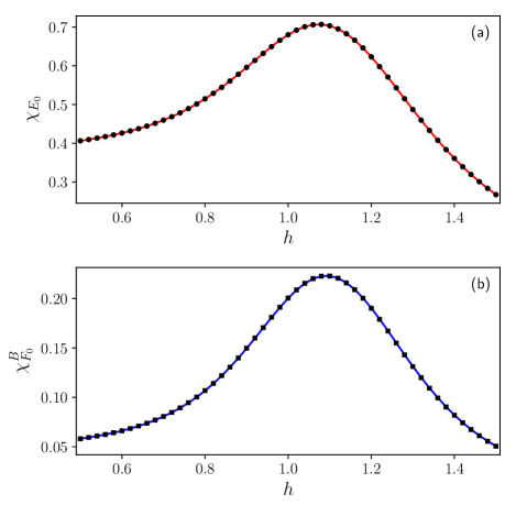
Figure 1: (Color online) Perturbative results of the NHTI chain at $\gamma=0.5$ with system size $N=10$ in biorthogonal bases. (a) Second derivatives of ground-state energy per site $\chi_{E_{0}}$, the red solid line denotes the results obtained by the five-point stencil method from Eq.(9) with ground state energy $E_{0}$, the circle symbols denote the results obtained from Eq.(10); (b) Biorthogonal ground-state fidelity susceptibility per site $\chi_{F_{0}}^{B}$, the blue solid line denotes the results from Eq.(16), the square symbols is given by Eq.(17).

III Fidelity Susceptibility

In this part, we develop the perturbation theory of the fidelity susceptibility. For non-Hermitian systems, we can introduce two types of fidelity susceptibility. First we can define a self-normal density matrix $\rho_{i}^{S}(\lambda)$ for $i$th eigenstates with only right eigenstates $|\psi_{i}^{R}(\lambda)\rangle$ (or only left eigenstates $|\psi_{i}^{L}(\lambda)\rangle$) as for Hermitian models,

$$\rho_{i}^{S}(\lambda)=|\psi_{i}^{R}(\lambda)\rangle\langle\psi_{i}^{R}(\lambda)|.$$ (11)

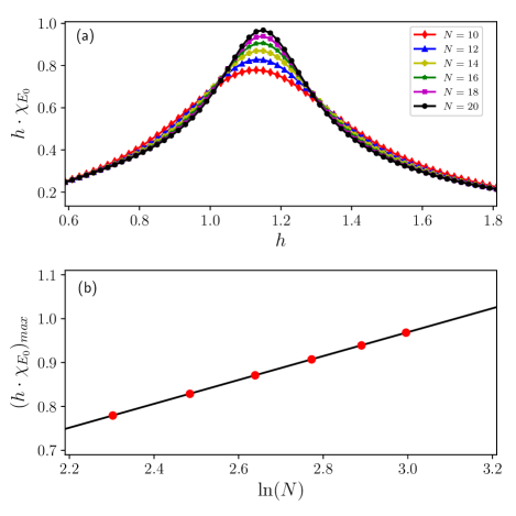
Figure 2: (Color online) Scaling of second derivatives of ground-state energy $\chi_{E_{0}}$ of the NHTI chain at $\gamma=0.5$. (a) Finite-size scaling of the $h\cdot\chi_{E_{0}}$ with system sizes from $N=10$ to $N=20$; (b) Finite-size scaling of the maxima of $h\cdot\chi_{E_{0}}$, where red circle symbols are the numerical results and the black solid line is the fitting curve.

Here the self-normal density matrix $\rho_{i}^{S}(\lambda)$ is a Hermitian matrix, $\rho_{i}^{S\dagger}(\lambda)=\rho_{i}^{S}(\lambda)$. However, the right eigenstates are non-orthonormal $\langle\psi_{i}^{R}(\lambda)|\psi_{j}^{R}(\lambda)\rangle\neq\delta_{ij}$ due to the non-hermiticity of systems although each of right eigenstates can be normalized $\langle\psi_{i}^{R}(\lambda)|\psi_{i}^{R}(\lambda)\rangle=1$ independently Brody (2013). Alternatively, we can define a biorthogonal density matrix $\rho_{i}^{B}(\lambda)$ from Eq.(5) by combining both right eigenstates $|\psi_{i}^{R}(\lambda)\rangle$ and left eigenstates $|\psi_{i}^{L}(\lambda)\rangle$ as Chang et al. (2020),

$$\rho_{i}^{B}(\lambda)=|\psi_{i}^{R}(\lambda)\rangle\langle\psi_{i}^{L}(\lambda)|,$$ (12)

where the biorthogonal density matrix $\rho_{i}^{B}(\lambda)$ is a non-Hermitian matrix, $\rho_{i}^{B\dagger}(\lambda)\neq\rho_{i}^{B}(\lambda)$. However, left and right eigenstates satisfy the bi-orthonormal relation and the completeness relation now.

Consequently, the Uhlmann fidelity

$$F_{i}=\text{Tr}\sqrt{\sqrt{\rho_{i}(\lambda)}\rho_{i}(\lambda+\delta\lambda)\sqrt{\rho_{i}(\lambda)}}$$ (13)

for the self-normal density matrix $\rho_{i}(\lambda)=\rho_{i}^{S}(\lambda)$ and the biorthogonal density matrix $\rho_{i}(\lambda)=\rho_{i}^{B}(\lambda)$ can be defined as Gu (2010); Uhlmann (1976); Hauru and Vidal (2018),

$$F_{i}^{S}= {}|\langle\psi_{i}^{R}(\lambda)|\psi_{i}^{R}(\lambda+\delta\lambda)\rangle|,$$ (14)

$$F_{i}^{B}= {}\sqrt{\langle\psi_{i}^{L}(\lambda+\delta\lambda)|\psi_{i}^{R}(\lambda)\rangle\langle\psi_{i}^{L}(\lambda)|\psi_{i}^{R}(\lambda+\delta\lambda)\rangle}.$$ (15)

The corresponding FS per site is then given by You et al. (2007); Albuquerque et al. (2010); Gu (2010); Sun (2017),

$$\chi_{F_{i}}^{S,B}=\frac{1}{N}\lim_{\delta\lambda\rightarrow 0}\frac{-2\ln F_{i}^{S,B}}{\delta\lambda^{2}}.$$ (16)

We note that the perturbation theory of the self-normal fidelity susceptibility $\chi_{F_{i}}^{S}$ was recently presented in Ref.[Matsumoto et al., 2020]. A symmetric definition of the biorthogonal fidelity susceptibility $\chi_{F_{i}}^{B}$ has already been introduced in Ref.[Jiang et al., 2018]. In this paper, we will focus mainly on the perturbation theory of biorthogonal fidelity susceptibility $\chi_{F_{i}}^{B}$ generalized from the Uhlmann fidelity. Using the standard perturbation theory, we obtain the following perturbative form of the biorthogonal fidelity susceptibility per site in Eq.(16) for $i$th eigenstates (see Appendix A for details),

$$\chi_{F_{i}}^{B}=\frac{1}{N}\sum_{n\neq i}\frac{\langle\psi_{i}^{L}(\lambda)|H^{\prime}|\psi_{n}^{R}(\lambda)\rangle\langle\psi_{n}^{L}(\lambda)|H^{\prime}|\psi_{i}^{R}(\lambda)\rangle}{[E_{i}(\lambda)-E_{n}(\lambda)]^{2}}.$$ (17)

This expression is numerically checked for a non-Hermitian transversed field Ising chain as follows.

Figure 3: (Color online) Fidelity susceptibility of the NHTI chain at $\gamma=0.5$. (a) Biorthogonal fidelity susceptibility $\chi_{F_{0}}^{B}$ with respect to $h$ for system sizes from $N=10$ to $N=20$; (b) Self-normal fidelity susceptibility $\chi_{F_{0}}^{S}$ as a function of $h$ with the same parameters as (a); (c) Finite-size scaling of the maxima of $\chi_{F_{0}}^{B}$ in (a); (d) Finite-size scaling of the maxima of $\chi_{F_{0}}^{S}$ in (b).

IV Model

As an example, we consider a one-dimensional non-Hermitian transversed field Ising (NHTI) model that was studied recently in Yang et al. (2020b); Von Gehlen (1991); Bianchini et al. (2014); Zhang and Song (2020),

$$H={} -\sum_{j=1}^{N}J\sigma_{j}^{x}\sigma_{j+1}^{x}+\sum_{j=1}^{N}h(\sigma_{j}^{z}+i\gamma\sigma_{j}^{y}).$$ (18)

Here $\sigma_{j}^{x},\sigma_{j}^{y},\sigma_{j}^{z}$ are Pauli matrices at the $j$th site, $N$ is the number of system site. The coupling strength $J>0$ and the amplitudes $h>0$, $\gamma\geq 0$ of the transversed fields are real numbers. The $i=\sqrt{-1}$ is the imaginary unit. For $\gamma=0$, the system is a Hermitian transversed field Ising model that undergoes a quantum phase transition at $h/J=1$ between the ferromagnetic (Ferro) phase for $h/J<1$ and the paramagnetic (Para) phase for $h/J>1$. For any $\gamma\neq 0$, the system is a NHTI model because of the imaginary transverse field term along the y-axis. The model has either all real eigenvalues for unbroken PT symmetry regimes $\gamma<1$ or complex conjugate pairs of eigenvalues for broken PT symmetry regimes $\gamma>1$, with a real-complex spectral transition at $\gamma_{c}=1$ (exceptional point) Yang et al. (2020b); Zhang and Song (2020). We are interested in the real eigenvalues regimes ($\gamma<1$) where the ground-state can be well defined as Hermitian models. In this unbroken PT symmetry regime, the system undergoes a biorthogonal order-disorder phase transition between the ferromagnetic phase and the paramagnetic phase at

$$h_{c}=\sqrt{\frac{1}{1-\gamma^{2}}}$$ (19)

in thermodynamic limit Yang et al. (2020b); Zhang and Song (2020). We will focus mainly on the finite-size scaling of the ground-state fidelity susceptibility near the critical points. We impose periodic boundary conditions $\sigma_{N+1}^{x}=\sigma_{1}^{x}$ and use $J=1$ in our numerical simulations.

We first calculate the second derivative of ground-state energy $\chi_{E_{0}}$ of Eq.(10) and the biorthogonal ground-state fidelity susceptibility $\chi_{F_{0}}^{B}$ of Eq.(17) by performing the exact diagonalization for the NHTI model from $N=10$ to $N=20$ sizes at $\gamma=0.5$ with the step $dh=10^{-3}$. The results of $\chi_{E_{0}}$ and $\chi_{F_{0}}^{B}$ obtained by Eq.(10) and Eq.(17) coincide exactly with that computed from the definitions in Eq.(9) and Eq.(16) directly [cf. Fig.1], indicating the perturbative formulas Eq.(8) and Eq.(17) we presented are valid. We find that the peak of second derivative of ground-state energy in the form of $h\cdot\chi_{E_{0}}$ increases with system sizes and diverges logarithmically [cf. Fig.2], implying that critical exponents $\alpha=0$ Chen et al. (2008); Um et al. (2007); You and Lu (2009).

We next discuss finite-size scaling of the biorthogonal and self-normal ground-state fidelity susceptibility $\chi_{F_{0}}^{B}$ and $\chi_{F_{0}}^{S}$ at $\gamma=0.5$ in detail. As demonstrated in Fig.3, both fidelity susceptibility display a nice peak that increase with system sizes. However, the finite-size scaling of $\chi_{F_{0}}^{B}$ and $\chi_{F_{0}}^{S}$ behave in a different way. For biorthogonal fidelity susceptibility $\chi_{F_{0}}^{B}$, a linear scaling is found [cf. Fig.3(c)]. That means we have the same correlation function critical exponents $\nu=1$ as Hermitian transversed field Ising chain according to the finite-size scaling of the ground-state fidelity susceptibility You et al. (2007); Albuquerque et al. (2010); Gu (2010); Sun (2017),

$$(\chi_{F_{0}}^{B})_{max}=N^{2/\nu-1},$$ (20)

for second-order phase transitions. For self-normal fidelity susceptibility $\chi_{F_{0}}^{S}$, a slow increase rate of the peak is observed [cf. Fig.3(d)]. In addition, the critical value $h_{c}$ obtained from the biorthogonal FS $\chi_{F_{0}}^{B}$ tends towards the exact value $h_{c}=2/\sqrt{3}\approx 1.1547$ in thermodynamic limit [cf. Fig.3(a) and Fig.4(b)]. For example, we get the critical point $h_{c}=1.1538$ in thermodynamic limit for $\gamma=0.5$ [see Fig.4(b)] by extrapolating data with Damski (2013)

$$h_{N}=h_{c}-a/N^{2}.$$ (21)

While the critical value $h_{c}$ derived from the self-normal FS $\chi_{F_{0}}^{S}$ gets worse and converges to $h_{c}=1.25$ when increasing the system size [cf. Fig.3(b) and Fig.4(b)].

We present the phase diagram in Fig.4(a) for $N=20$, where it is clear that the biorthogonal FS $\chi_{F_{0}}^{B}$ instead of the self-normal FS $\chi_{F_{0}}^{S}$ characterizes the biorthogonal order-disorder phase transitions. The critical exponents $\alpha=0$ and $\nu=1$ derived from the finite-size scaling indicate the biorthogonal phase transitions of the NHTI model is a second-order phase transition with the Ising universal class.

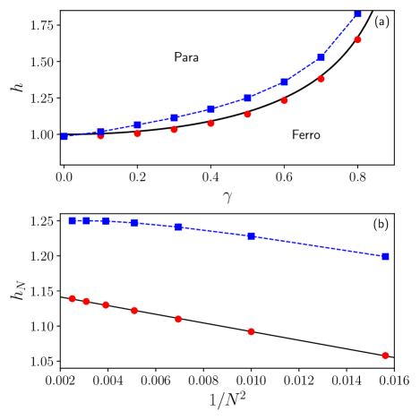
Figure 4: (Color online) Phase diagram of the NHTI chain. (a) Full phase diagram; Red circle symbols denote the critical values $h_{N}$ obtained from the biorthogonal FS $\chi_{F_{0}}^{B}$ for system size $N=20$; Blue square symbols are derived self-normal FS $\chi_{F_{0}}^{S}$ for system size $N=20$; the black solid line is the exact result. (b) Blue square symbols and Red circle symbols denote the finite-size scaling of critical value $h_{N}$ at the maxima of the self-normal FS $\chi_{F_{0}}^{S}$ and the biorthogonal FS $\chi_{F_{0}}^{B}$ for $\gamma=0.5$; the black solid line is the fitting curve with the $h_{c}=1.1538$ from biorthogonal FS $\chi_{F_{0}}^{B}$.

V Conclusion

In summary, we have studied the perturbation theory of the biorthogonal fidelity susceptibility and the biorthogonal quantum criticality in interacting non-Hermitian many-body systems. We have shown that the second derivative of ground-state energy and the biorthogonal ground-state fidelity susceptibility can serve as probes to detect quantum phase transitions and the corresponding critical exponents of non-Hermitian many-body systems. We show that the biorthogonal fidelity susceptibility instead of the conventional self-normal fidelity susceptibility should be used to characterize phase transitions associated with the energy levels (i.e. level crossing) because the non-Hermitian Hamiltonian is diagonal in biorthogonal basis.

We note that the concept of the biorthogonal fidelity susceptibility in Eq.(16) and its perturbative form as shown in Eq.(17) are general for any non-Hermitian many-body Hamiltonian with real eigenvalues. Consequently, it would be possible to apply the biorthogonal fidelity susceptibility to understand the nature of phase transitions in non-integrable non-Hermitian many-body models. Moreover, it would be more interesting to know whether the biorthogonal fidelity susceptibility is useful to detect the universal class for the real-complex spectral transition of non-Hermitian many-body models Chang et al. (2020) or the localization-delocalization transition of a non-Hermitian quantum systems Hatano and Obuse (2021); Liu et al. (2021); Lin et al. (2021) in the future.

Appendix A Perturbation theory of biorthogonal fidelity susceptibility

Assume we know the eigenvalues $E_{i}(\lambda)$ and the left and right eigenvectors $|\psi_{i}^{L}(\lambda)\rangle$ and $|\psi_{i}^{R}(\lambda)\rangle$ of a Hamiltonian $H(\lambda)$. According to the perturbation theory of non-Hermitian systems, the left and right eigenvectors $|\psi_{i}^{L}(\lambda+\delta\lambda)\rangle$ and $|\psi_{i}^{R}(\lambda+\delta\lambda)\rangle$ of the Hamiltonian $H(\lambda+\delta\lambda$) can be expanded in powers of $\delta\lambda$ as Matsumoto et al. (2020); Gu (2010); Chen et al. (2008),

$$\langle\psi_{i}^{L}(\lambda+\delta\lambda)|=c_{1}\left[\langle\psi_{i}^{L}(\lambda)|+\delta\lambda\sum_{n\neq i}\frac{H_{in}^{\prime}\langle\psi_{n}^{L}(\lambda)|}{E_{i}(\lambda)-E_{n}(\lambda)}\right],$$ (22)

$$|\psi_{i}^{R}(\lambda+\delta\lambda)\rangle=c_{2}\left[|\psi_{i}^{R}(\lambda)\rangle+\delta\lambda\sum_{n\neq i}\frac{H_{ni}^{\prime}|\psi_{n}^{R}(\lambda)\rangle}{E_{i}(\lambda)-E_{n}(\lambda)}\right],$$ (23)

up to the first order. Where $H_{ni}^{\prime}=\langle\psi_{n}^{L}(\lambda)|H^{\prime}|\psi_{i}^{R}(\lambda)\rangle$, $c_{1}=\langle\psi_{i}^{L}(\lambda+\delta\lambda)|\psi_{i}^{R}(\lambda)\rangle$ and $c_{2}=\langle\psi_{i}^{L}(\lambda)|\psi_{i}^{R}(\lambda+\delta\lambda)\rangle$ are the normalization constants. We can get the biorthogonal fidelity susceptibility $F_{i}^{B}$ in terms of the $c_{1}$ and $c_{2}$ by multiplying equation (22) by right eigenvectors $|\psi_{i}^{R}(\lambda)\rangle$ and multiplying equation (23) by the left eigenvectors $\langle\psi_{i}^{L}(\lambda)|$ respectively,

$$(F_{i}^{B})^{2}= {}\langle\psi_{i}^{L}(\lambda+\delta\lambda)|\psi_{i}^{R}(\lambda)\rangle\langle\psi_{i}^{L}(\lambda)|\psi_{i}^{R}(\lambda+\delta\lambda)\rangle$$

$$= {}c_{1}c_{2}$$ (24)

Multiplying equation (22) by equation (23) and using the normalization condition $\langle\psi_{i}^{L}(\lambda+\delta\lambda)|\psi_{i}^{R}(\lambda+\delta\lambda)\rangle=1,$ we derive the equation of biorthogonal fidelity,

$$1=(F_{i}^{B})^{2}\left[1+(\delta\lambda)^{2}\sum_{n\neq i}\frac{H_{in}^{\prime}H_{ni}^{\prime}}{[E_{i}(\lambda)-E_{n}(\lambda)]^{2}}\right].$$ (25)

Where the Eq.(24) has been used. The biorthogonal fidelity susceptibility per site can be obtained as,

$$\chi_{F_{i}}^{B}=\frac{1}{N}\sum_{n\neq i}\frac{\langle\psi_{i}^{L}(\lambda)|H^{\prime}|\psi_{n}^{R}(\lambda)\rangle\langle\psi_{n}^{L}(\lambda)|H^{\prime}|\psi_{i}^{R}(\lambda)\rangle}{[E_{i}(\lambda)-E_{n}(\lambda)]^{2}}.$$ (26)

by considering the leading term to second-order.

Appendix B Differential form of biorthogonal fidelity susceptibility

Next we will derive the differential form of the biorthogonal FS $\chi_{F_{i}}^{B}$ for the $i$th state. The left and right eigenvectors $|\psi_{i}^{L}(\lambda+\delta\lambda)\rangle$ and $|\psi_{i}^{R}(\lambda+\delta\lambda)\rangle$ of the Hamiltonian $H(\lambda+\delta\lambda$) are firstly expanded using Taylor series in powers of $\delta\lambda$ as Matsumoto et al. (2020); Gu (2010); Chen et al. (2008),

$$\langle\psi_{i}^{L}(\lambda+\delta\lambda)|={} \langle\psi_{i}^{L}(\lambda)|+\delta\lambda\langle\partial_{\lambda}\psi_{i}^{L}(\lambda)|$$

$$~{}~{}+\frac{\delta\lambda^{2}}{2}\langle\partial^{2}_{\lambda}\psi_{i}^{L}(\lambda)|+O(\delta\lambda^{3}),$$ (27)

$$|\psi_{i}^{R}(\lambda+\delta\lambda)\rangle={} |\psi_{i}^{R}(\lambda)\rangle+\delta\lambda|\partial_{\lambda}\psi_{i}^{R}(\lambda)\rangle$$

$$~{}~{}+\frac{\delta\lambda^{2}}{2}|\partial^{2}_{\lambda}\psi_{i}^{R}(\lambda)\rangle+O(\delta\lambda^{3}),$$ (28)

Hence the overlap $\langle\psi_{i}^{L}(\lambda+\delta\lambda)|\psi_{i}^{R}(\lambda)\rangle$ and $\langle\psi_{i}^{L}(\lambda)|\psi_{i}^{R}(\lambda+\delta\lambda)\rangle$ are given as,

$$\langle\psi_{i}^{L}(\lambda+\delta\lambda)|\psi_{i}^{R}(\lambda)\rangle={} 1+\delta\lambda\langle\partial_{\lambda}\psi_{i}^{L}(\lambda)|\psi_{i}^{R}(\lambda)\rangle$$

$$~{}~{}+\frac{\delta\lambda^{2}}{2}\langle\partial_{\lambda}^{2}\psi_{i}^{L}(\lambda)|\psi_{i}^{R}(\lambda)\rangle$$ (29)

$$\langle\psi_{i}^{L}(\lambda)|\psi_{i}^{R}(\lambda+\delta\lambda)\rangle={} 1+\delta\lambda\langle\psi_{i}^{L}(\lambda)|\partial_{\lambda}\psi_{i}^{R}(\lambda)\rangle$$

$$~{}~{}+\frac{\delta\lambda^{2}}{2}\langle\psi_{i}^{L}(\lambda)|\partial_{\lambda}^{2}\psi_{i}^{R}(\lambda)\rangle,$$ (30)

Where the bi-orthonormal relation $\langle\psi_{i}^{L}(\lambda)|\psi_{i}^{R}(\lambda)\rangle=1$ is used. From Eq.(24), we have

$$(F_{i}^{B})^{2}={} \langle\psi_{i}^{L}(\lambda+\delta\lambda)|\psi_{i}^{R}(\lambda)\rangle\langle\psi_{i}^{L}(\lambda)|\psi_{i}^{R}(\lambda+\delta\lambda)\rangle$$

$$={} 1+\delta\lambda\left[\langle\partial_{\lambda}\psi_{i}^{L}(\lambda)|\psi_{i}^{R}(\lambda)\rangle+\langle\psi_{i}^{L}(\lambda)|\partial_{\lambda}\psi_{i}^{R}(\lambda)\rangle\right]$$

$$~{}~{}+\frac{\delta\lambda^{2}}{2}\left[2\langle\partial_{\lambda}\psi_{i}^{L}(\lambda)|\psi_{i}^{R}(\lambda)\rangle\langle\psi_{i}^{L}(\lambda)|\partial_{\lambda}\psi_{i}^{R}(\lambda)\rangle\right.$$

$$~{}~{}~{}~{}~{}~{}~{}~{}+\left.\langle\partial_{\lambda}^{2}\psi_{i}^{L}(\lambda)|\psi_{i}^{R}(\lambda)\rangle+\langle\psi_{i}^{L}(\lambda)|\partial_{\lambda}^{2}\psi_{i}^{R}(\lambda)\rangle\right]$$ (31)

up to the second order of $\delta\lambda^{2}$. From the bi-orthonormal relation $\langle\psi_{i}^{L}(\lambda)|\psi_{i}^{R}(\lambda)\rangle=1$, we can get

$$\partial_{\lambda}\langle\psi_{i}^{L}(\lambda)|\psi_{i}^{R}(\lambda)\rangle={} \langle\partial_{\lambda}\psi_{i}^{L}(\lambda)|\psi_{i}^{R}(\lambda)\rangle+\langle\psi_{i}^{L}(\lambda)|\partial_{\lambda}\psi_{i}^{R}(\lambda)\rangle$$

$$={} 0$$ (32)

$$\partial_{\lambda}^{2}\langle\psi_{i}^{L}(\lambda)|\psi_{i}^{R}(\lambda)\rangle={} \langle\partial_{\lambda}^{2}\psi_{i}^{L}(\lambda)|\psi_{i}^{R}(\lambda)\rangle+\langle\psi_{i}^{L}(\lambda)|\partial_{\lambda}^{2}\psi_{i}^{R}(\lambda)\rangle$$

$$~{}~{}+2\langle\partial_{\lambda}\psi_{i}^{L}(\lambda)|\partial_{\lambda}\psi_{i}^{R}(\lambda)\rangle$$

$$={} 0$$ (33)

Using the relations Eq.(32) and Eq.(33), the Eq.(31) becomes

$$(F_{i}^{B})^{2}={} 1-\delta\lambda^{2}N\chi_{F_{i}}^{B},$$ (34)

where the biorthogonal FS per site $\chi_{F_{i}}^{B}$ is defined as

$$\chi_{F_{i}}^{B}=\frac{1}{N}{} \left[\langle\partial_{\lambda}\psi_{i}^{L}(\lambda)|\partial_{\lambda}\psi_{i}^{R}(\lambda)\rangle\right.$$

$$-\left.\langle\partial_{\lambda}\psi_{i}^{L}(\lambda)|\psi_{i}^{R}(\lambda)\rangle\langle\psi_{i}^{L}(\lambda)|\partial_{\lambda}\psi_{i}^{R}(\lambda)\rangle\right].$$ (35)

References

- Sachdev (1999) S. Sachdev, Quantum phase transitions (Cambridge University Press, 1999).
- Levin and Wen (2006) M. Levin and X.-G. Wen, Physical review letters 96, 110405 (2006).
- Fisher and Barber (1972) M. E. Fisher and M. N. Barber, Physical leview letters 28, 1516 (1972).
- Fisher (1974) M. E. Fisher, Reviews of Modern Physics 46, 597 (1974).
- Bergholtz et al. (2021) E. J. Bergholtz, J. C. Budich, and F. K. Kunst, Reviews of Modern Physics 93, 015005 (2021).
- Ashida et al. (2020) Y. Ashida, Z. Gong, and M. Ueda, Advances in Physics 69, 249 (2020).
- Lee (2016) T. E. Lee, Physical review letters 116, 133903 (2016).
- Yao and Wang (2018) S. Yao and Z. Wang, Physical review letters 121, 086803 (2018).
- Kunst et al. (2018) F. K. Kunst, E. Edvardsson, J. C. Budich, and E. J. Bergholtz, Physical review letters 121, 026808 (2018).
- Xiong (2018) Y. Xiong, Journal of Physics Communications 2, 035043 (2018).
- Gong et al. (2018) Z. Gong, Y. Ashida, K. Kawabata, K. Takasan, S. Higashikawa, and M. Ueda, Physical Review X 8, 031079 (2018).
- Martinez Alvarez et al. (2018) V. M. Martinez Alvarez, J. E. Barrios Vargas, and L. E. F. Foa Torres, Physical Review B 97, 121401(R) (2018).
- Yokomizo and Murakami (2019) K. Yokomizo and S. Murakami, Physical review letters 123, 066404 (2019).
- Okuma et al. (2020) N. Okuma, K. Kawabata, K. Shiozaki, and M. Sato, Physical review letters 124, 086801 (2020).
- Zhang et al. (2020a) K. Zhang, Z. Yang, and C. Fang, Physical review letters 125, 126402 (2020a).
- Yang et al. (2020a) Z. Yang, K. Zhang, C. Fang, and J. Hu, Physical Review Letters 125, 226402 (2020a).
- Wang et al. (2020) X.-R. Wang, C.-X. Guo, and S.-P. Kou, Physical Review B 101, 121116(R) (2020).
- Jiang et al. (2020) H. Jiang, R. Lü, and S. Chen, The European Physical Journal B 93, 1 (2020).
- Weidemann et al. (2020) S. Weidemann, M. Kremer, T. Helbig, T. Hofmann, A. Stegmaier, M. Greiter, R. Thomale, and A. Szameit, Science 368, 311 (2020).
- Xiao et al. (2020) L. Xiao, T. Deng, K. Wang, G. Zhu, Z. Wang, W. Yi, and P. Xue, Nature Physics , 1 (2020).
- Borgnia et al. (2020) D. S. Borgnia, A. J. Kruchkov, and R.-J. Slager, Physical review letters 124, 056802 (2020).
- Heiss (2012) W. Heiss, Journal of Physics A: Mathematical and Theoretical 45, 444016 (2012).
- Kozii and Fu (2017) V. Kozii and L. Fu, arXiv preprint arXiv:1708.05841 (2017).
- Hodaei et al. (2017) H. Hodaei, A. U. Hassan, S. Wittek, H. Garcia-Gracia, R. El-Ganainy, D. N. Christodoulides, and M. Khajavikhan, Nature 548, 187 (2017).
- Zhou et al. (2018) H. Zhou, C. Peng, Y. Yoon, C. W. Hsu, K. A. Nelson, L. Fu, J. D. Joannopoulos, M. Soljačić, and B. Zhen, Science 359, 1009 (2018).
- Miri and Alu (2019) M.-A. Miri and A. Alu, Science 363, aar7709 (2019).
- Park et al. (2019) J.-H. Park, A. Ndao, W. Cai, L.-Y. Hsu, A. Kodigala, T. Lepetit, Y.-H. Lo, and B. Kanté, arXiv preprint arXiv:1904.01073 (2019).
- Yang and Hu (2019) Z. Yang and J. Hu, Physical Review B 99, 081102(R) (2019).
- Özdemir et al. (2019) Ş. Özdemir, S. Rotter, F. Nori, and L. Yang, Nature materials 18, 783 (2019).
- Dóra et al. (2019) B. Dóra, M. Heyl, and R. Moessner, Nature communications 10, 1 (2019).
- Zhang et al. (2019) Y.-R. Zhang, Z.-Z. Zhang, J.-Q. Yuan, M. Kang, and J. Chen, Frontiers of Physics 14, 53603 (2019).
- Jin et al. (2020) L. Jin, H. C. Wu, B.-B. Wei, and Z. Song, Physical Review B 101, 045130 (2020).
- Xiao et al. (2021) L. Xiao, T. Deng, K. Wang, Z. Wang, W. Yi, and P. Xue, Physical Review Letters 126, 230402 (2021).
- Matsumoto et al. (2020) N. Matsumoto, K. Kawabata, Y. Ashida, S. Furukawa, and M. Ueda, Physical Review Letters 125, 260601 (2020).
- Yang et al. (2020b) M.-L. Yang, H. Wang, C.-X. Guo, X.-R. Wang, G. Sun, and S.-P. Kou, arXiv preprint arXiv:2006.10278 (2020b).
- Jin and Song (2013) L. Jin and Z. Song, Annals of Physics 330, 142 (2013).
- Ashida et al. (2017) Y. Ashida, S. Furukawa, and M. Ueda, Nature communications 8, 1 (2017).
- Herviou et al. (2019) L. Herviou, N. Regnault, and J. H. Bardarson, SciPost Physics 7 (2019), 10.21468/SciPostPhys.7.5.069.
- Chang et al. (2020) P.-Y. Chang, J.-S. You, X. Wen, and S. Ryu, Physical Review Research 2, 033069 (2020).
- Mu et al. (2020) S. Mu, C. H. Lee, L. Li, and J. Gong, Physical Review B 102, 081115(R) (2020).
- Lee et al. (2020) E. Lee, H. Lee, and B.-J. Yang, Physical Review B 101, 121109(R) (2020).
- Pan et al. (2020a) L. Pan, X. Chen, Y. Chen, and H. Zhai, Nature Physics 16, 767 (2020a).
- Pan et al. (2020b) L. Pan, X. Wang, X. Cui, and S. Chen, Physical Review A 102, 023306 (2020b).
- Xu and Chen (2020) Z. Xu and S. Chen, Physical Review B 102, 035153 (2020).
- Zhang et al. (2020b) D.-W. Zhang, Y.-L. Chen, G.-Q. Zhang, L.-J. Lang, Z. Li, and S.-L. Zhu, Physical Review B 101, 235150 (2020b).
- Lee (2020) C. H. Lee, arXiv preprint arXiv:2006.01182 (2020).
- Shackleton and Scheurer (2020) H. Shackleton and M. S. Scheurer, Physical Review Research 2, 033022 (2020).
- Liu et al. (2020) T. Liu, J. J. He, T. Yoshida, Z.-L. Xiang, and F. Nori, Physical Review B 102, 235151 (2020).
- Yang et al. (2021) K. Yang, S. C. Morampudi, and E. J. Bergholtz, Physical Review Letters 126, 077201 (2021).
- Hanai et al. (2019) R. Hanai, A. Edelman, Y. Ohashi, and P. B. Littlewood, Physical review letters 122, 185301 (2019).
- Hamazaki et al. (2019) R. Hamazaki, K. Kawabata, and M. Ueda, Physical review letters 123, 090603 (2019).
- Xi et al. (2021) W. Xi, Z.-H. Zhang, Z.-C. Gu, and W.-Q. Chen, Science Bulletin (2021), https://doi.org/10.1016/j.scib.2021.04.027.
- Yamamoto et al. (2019) K. Yamamoto, M. Nakagawa, K. Adachi, K. Takasan, M. Ueda, and N. Kawakami, Physical Review Letters 123, 123601 (2019).
- Hanai and Littlewood (2020) R. Hanai and P. B. Littlewood, Physical Review Research 2, 033018 (2020).
- Arouca et al. (2020) R. Arouca, C. H. Lee, and C. M. Smith, Physical Review B 102, 245145 (2020).
- Zanardi and Paunković (2006) P. Zanardi and N. Paunković, Physical Review E 74, 031123 (2006).
- Campos Venuti and Zanardi (2007) L. Campos Venuti and P. Zanardi, Physical Review Letters 99, 095701 (2007).
- You et al. (2007) W.-L. You, Y.-W. Li, and S.-J. Gu, Physical Review E 76, 022101 (2007).
- Albuquerque et al. (2010) A. F. Albuquerque, F. Alet, C. Sire, and S. Capponi, Physical Review B 81, 064418 (2010).
- Gu (2010) S.-J. Gu, International Journal of Modern Physics B 24, 4371 (2010).
- Sun (2017) G. Sun, Physical Review A 96, 043621 (2017).
- Zhu et al. (2018) Z. Zhu, G. Sun, W.-L. You, and D.-N. Shi, Physical Review A 98, 023607 (2018).
- Wei and Lv (2018) B.-B. Wei and X.-C. Lv, Physical Review A 97, 013845 (2018).
- Wei (2019) B.-B. Wei, Physical Review A 99, 042117 (2019).
- Chen et al. (2008) S. Chen, L. Wang, Y. Hao, and Y. Wang, Physical Review A 77, 032111 (2008).
- Gu et al. (2008) S.-J. Gu, H.-M. Kwok, W.-Q. Ning, and H.-Q. Lin, Physical Review B 77, 245109 (2008).
- Yang et al. (2008) S. Yang, S.-J. Gu, C.-P. Sun, and H.-Q. Lin, Physical Review A 78, 012304 (2008).
- Kwok et al. (2008) H.-M. Kwok, W.-Q. Ning, S.-J. Gu, and H.-Q. Lin, Physical Review E 78, 032103 (2008).
- Gong and Tong (2008) L. Gong and P. Tong, Physical Review B 78, 115114 (2008).
- Yu et al. (2009) W.-C. Yu, H.-M. Kwok, J. Cao, and S.-J. Gu, Physical Review E 80, 021108 (2009).
- Schwandt et al. (2009) D. Schwandt, F. Alet, and S. Capponi, Physical Review letters 103, 170501 (2009).
- Luo et al. (2018) Q. Luo, J. Zhao, and X. Wang, Physical Review E 98, 022106 (2018).
- Rams and Damski (2011) M. M. Rams and B. Damski, Physical Review letters 106, 055701 (2011).
- Li et al. (2012) S.-H. Li, Q.-Q. Shi, Y.-H. Su, J.-H. Liu, Y.-W. Dai, and H.-Q. Zhou, Physical Review B 86, 064401 (2012).
- Mukherjee et al. (2012) V. Mukherjee, A. Dutta, and D. Sen, Physical Review B 85, 024301 (2012).
- Damski (2013) B. Damski, Physical Review E 87, 052131 (2013).
- Carrasquilla et al. (2013) J. Carrasquilla, S. R. Manmana, and M. Rigol, Physical Review A 87, 043606 (2013).
- Łącki et al. (2014) M. Łącki, B. Damski, and J. Zakrzewski, Physical Review A 89, 033625 (2014).
- Sun and Vekua (2016) G. Sun and T. Vekua, Physical Review B 93, 205137 (2016).
- Yang (2007) M.-F. Yang, Physical Review B 76, 180403(R) (2007).
- Fjærestad (2008) J. O. Fjærestad, Journal of Statistical Mechanics: Theory and Experiment 2008, P07011 (2008).
- Langari and Rezakhani (2012) A. Langari and A. Rezakhani, New Journal of Physics 14, 053014 (2012).
- Sun et al. (2015) G. Sun, A. K. Kolezhuk, and T. Vekua, Physical Review B 91, 014418 (2015).
- Cincio et al. (2019) L. Cincio, M. M. Rams, J. Dziarmaga, and W. H. Zurek, Physical Review B 100, 081108(R) (2019).
- Sun et al. (2019) G. Sun, B.-B. Wei, and S.-P. Kou, Physical Review B 100, 064427 (2019).
- Jiang et al. (2018) H. Jiang, C. Yang, and S. Chen, Physical Review A 98, 052116 (2018).
- Wang et al. (2019) C. Wang, M.-L. Yang, C.-X. Guo, X.-M. Zhao, and S.-P. Kou, EPL (Europhysics Letters) 128, 41001 (2019).
- Guo et al. (2020) C.-X. Guo, X.-R. Wang, and S.-P. Kou, EPL (Europhysics Letters) 131, 27002 (2020).
- Nishiyama (2020a) Y. Nishiyama, Physica A: Statistical Mechanics and its Applications , 124731 (2020a).
- Nishiyama (2020b) Y. Nishiyama, The European Physical Journal B 93, 1 (2020b).
- Tzeng et al. (2021) Y.-C. Tzeng, C.-Y. Ju, G.-Y. Chen, and W.-M. Huang, Physical Review Research 3, 013015 (2021).
- Solnyshkov et al. (2021) D. D. Solnyshkov, C. Leblanc, L. Bessonart, A. Nalitov, J. Ren, Q. Liao, F. Li, and G. Malpuech, Physical Review B 103, 125302 (2021).
- Brody (2013) D. C. Brody, Journal of Physics A: Mathematical and Theoretical 47, 035305 (2013).
- Sternheim and Walker (1972) M. M. Sternheim and J. F. Walker, Physical Review C 6, 114 (1972).
- Mostafazadeh (2002a) A. Mostafazadeh, Journal of Mathematical Physics 43, 205 (2002a).
- Mostafazadeh (2002b) A. Mostafazadeh, Journal of Mathematical Physics 43, 2814 (2002b).
- Mostafazadeh (2002c) A. Mostafazadeh, Journal of Mathematical Physics 43, 3944 (2002c).
- Fu et al. (2019) Y.-Y. Fu, Y. Fei, D.-X. Dong, and Y.-W. Liu, Frontiers of Physics 14, 62601 (2019).
- Zhao (2020) Y. Zhao, Frontiers of Physics 15, 13603 (2020).
- Chen et al. (2021) Y.-C. Chen, M. Gong, P. Xue, H.-D. Yuan, and C.-J. Zhang, Frontiers of Physics 16, 53601 (2021).
- Uhlmann (1976) A. Uhlmann, Reports on Mathematical Physics 9, 273 (1976).
- Hauru and Vidal (2018) M. Hauru and G. Vidal, Physical Review A 98, 042316 (2018).
- Von Gehlen (1991) G. Von Gehlen, Journal of Physics A: Mathematical and General 24, 5371 (1991).
- Bianchini et al. (2014) D. Bianchini, O. Castro-Alvaredo, B. Doyon, E. Levi, and F. Ravanini, Journal of Physics A: Mathematical and Theoretical 48, 04FT01 (2014).
- Zhang and Song (2020) K. L. Zhang and Z. Song, Physical Review B 101, 245152 (2020).
- Um et al. (2007) J. Um, S.-I. Lee, and B. J. Kim, J. Korean Phy. Soc. 50, 285 (2007).
- You and Lu (2009) W.-L. You and W.-L. Lu, Physics Letters A 373, 1444 (2009).
- Hatano and Obuse (2021) N. Hatano and H. Obuse, Annals of Physics , 168615 (2021).
- Liu et al. (2021) T. Liu, S. Cheng, H. Guo, and G. Xianlong, Physical Review B 103, 104203 (2021).
- Lin et al. (2021) Q. Lin, T. Li, L. Xiao, K. Wang, W. Yi, and P. Xue, arXiv preprint arXiv:2108.01097 (2021).