Towards accelerated rates for distributed optimization over time-varying networks

Abstract

We study the problem of decentralized optimization with strongly convex smooth cost functions. This paper investigates accelerated algorithms under time-varying network constraints. In our approach, nodes run a multi-step gossip procedure after taking each gradient update, thus ensuring approximate consensus at each iteration. The outer cycle is based on accelerated Nesterov scheme. Both computation and communication complexities of our method have an optimal dependence on global function condition number $\kappa_{g}$. In particular, the algorithm reaches an optimal computation complexity $O(\sqrt{\kappa_{g}}\log(1/\varepsilon))$.

Keywords distributed optimization  $\cdot$ time-varying network

1 Introduction

In this work, we study a sum-type minimization problem

$$f(x)=\frac{1}{n}\sum_{i=1}^{n}f_{i}(x)\to\min_{x\in\mathbb{R}^{d}}.$$ (1)

Convex functions $f_{i}$ are stored separately by nodes in communication network, which is represented by an undirected graph $\mathcal{G}=(V,E)$. This type of problems arise in distributed machine learning, drone or satellite networks, statistical inference [1] and power system control [2]. The computational agents over the network have access to their local $f_{i}$ and can communicate only with their neighbors, but still aim to minimize the global objective in (1).

The basic idea behind approach of this paper is to reformulate problem (1) as a problem with linear constraints. Let us assign each agent in the network a personal copy of parameter vector $x_{i}$ and introduce

$${\bf X}=\begin{pmatrix}x_{1}^{\top}\\ \vdots\\ x_{n}^{\top}\end{pmatrix}\in\mathbb{R}^{n\times d},\leavevmode\nobreak\ F({\bf X})=\sum_{i=1}^{n}f_{i}(x_{i}).$$

Now we equivalently rewrite problem (1) as

$$F({\bf X})=\sum_{i=1}^{n}f_{i}(x_{i})\to\min_{x_{1}=\ldots=x_{n}}.$$ (2)

This reformulation increases the number of variables, but induces additional constraints at the same time. Problem (2) has the same optimal value as problem (1).

Let us denote the set of consensus constraints $\mathcal{C}=\{x_{1}=\ldots=x_{n}\}$. Also, for each ${\bf X}\in\mathbb{R}^{d\times n}$ denote average of its columns $\overline{x}=\frac{1}{n}\sum_{i=1}^{n}x_{i}$ and introduce its projection onto constraint set.

$$\overline{\bf X}=\frac{1}{n}\mathbf{1}_{n}\mathbf{1}_{n}^{\top}{\bf X}=\Pi_{\mathcal{C}}({\bf X})=\begin{pmatrix}\overline{x}^{\top}\\ \vdots\\ \overline{x}^{\top}\end{pmatrix}.$$

Note that $\mathcal{C}$ is a linear subspace in $\mathbb{R}^{n\times d}$, and therefore projection operator $\Pi_{\mathcal{C}}(\cdot)$ is linear.

Decentralized optimization methods aim at minimizing the objective function and maintaining consensus accuracy between nodes. The optimization part is performed by using gradient steps. At the same time, keeping every agent’s parameter vector close to average over the nodes is done via communication steps. Alternating gradient and communication updates allows both to minimize the objective and control consensus constraint violation.

In centralized scenario, there exists a server which is able to communicate with every agent in the network. In particular, a common parameter vector is maintained at all of the nodes. However, in decentralized setting it is only possible to ensure that agent’s vectors are approximately equal with desired accuracy. The algorithm studied in this paper runs a sequence of communication rounds after every optimization step. We refer to this series of communications as consensus subroutine. Such information exchange allows to reach approximate consensus between nodes after each gradient update, while the accuracy is controlled by the number of communication rounds.

On the one hand, a method which employs a consensus subroutine after each gradient update mimics a centralized algorithm. The difference is that in presence of a master node all computational entities have access to a common variable, while in decentralized case consensus constraints are satisfied only with nonzero accuracy. On the other hand, consensus subroutine may be interpreted as an inexact projection onto the constraint set $\mathcal{C}$. Every communication round is a step towards the projection. Therefore, our approach fits the inexact oracle framework, which has been studied in [3, 4]. We note that a similar approach to decentralized optimization is studied in [5].

We aim at building a first-order method with trajectory lying in neighborhood of $\mathcal{C}$. A simple example would be GD with inexact projections.

$${\bf X}^{k+1}\approx\Pi_{\mathcal{C}}({\bf X}^{k}-\gamma\nabla F({\bf X}^{k}))=\overline{\bf X}^{k}-\gamma\overline{\nabla F}({\bf X}^{k}),$$ (3)

where $\nabla F({\bf X}^{k})=(\nabla f_{1}(x_{1}^{k})\ldots\nabla f_{n}(x_{n}^{k}))^{\top}$ denotes the gradient of $F$.

Algorithm with update rule 3 can be viewed as a gradient descent with inexact oracle. If the oracle was exact, the update rule would write as

$$\overline{\bf X}^{k+1}=\overline{\bf X}^{k}-\gamma\overline{\nabla F}(\overline{\bf X}^{k}),$$

thus making the method trajectory stay precisely in $\mathcal{C}$. In this particular example, inexact gradient $\overline{\nabla F}({\bf X}^{k})$ approximates exact gradient $\overline{\nabla F}(\overline{\bf X}^{k})$.

Throughout the paper, $\left\langle\cdot,\cdot\right\rangle$ denotes the inner product of vectors or matrices. Correspondingly, by $\left\|\cdot\right\|$ we denote a $2$-norm for vectors or Frobenius norm for matrices.

1.1 Related work

A decentralized algorithm makes two types of steps: local updates and information exchange. The complexity of such methods depends on objective condition number $\kappa$ and a term $\chi$ representing graph connectivity.

Local steps may use gradient [6, 7, 8, 9, 10, 11, 12] or sub-gradient [13] computations. In primal-only methods, the agents compute gradients of their local functions and alternate taking gradient steps and communication procedures. Under cheap communication costs, it may be beneficial to replace a single consensus iteration with a series of information exchange rounds. Such methods as MSDA [14], D-NC [15] and Mudag [11] employ multi-step gossip procedures.

Typically, non-accelerated methods need $O(\kappa\chi\log(1/\varepsilon))$ iterations to yield a solution with $\varepsilon$-accuracy [16]. Nesterov acceleration may be employed to improve dependence on $\kappa$ or $\chi$ and obtain algorithms with $O(\sqrt{\kappa\chi}\log(1/\varepsilon))$ complexity. In order to achieve this, one may distribute accelerated methods directly [9, 11, 12, 15, 17] or use a Catalyst framework [18]. Accelerated methods meet the lower complexity bounds for decentralized optimization [19, 20, 14].

Consensus restrictions $x_{1}=\ldots=x_{n}$ may be treated as linear constraints, thus allowing for a dual reformulation of problem (1). Dual-based methods include dual ascent and its accelerated variants [14, 21, 22, 23]. Primal-dual approaches like ADMM [24, 25] are also implementable in decentralized scenarios.

In [7], the authors developed algorithms for non-smooth convex objectives and provided lower complexity bounds for non-smooth convex case, as well.

Time-varying networks open a new venue in research. Changing topology requires new approaches to decentralized methods and a more complicated theoretical analysis. The first method with provable geometric convergence was proposed in [6]. Such primal algorithms as Push-Pull Gradient Method [8] and DIGing [6] are robust to network changes and have theoretical guarantees of convergence over time-varying graphs. Recently, a dual method for time-varying architectures was introduced in [26].

1.2 Summary of contributions

Our approach uses multi-step gossip averaging, and the analysis is based on the inexact oracle framework.

The proposed algorithm (Algorithm 1) requires $O(\sqrt{\kappa_{g}}\chi\log^{2}(1/\varepsilon))$, where $\kappa_{g}$ denotes the (global) condition number of $f$ and $\chi$ is a term characterizing graph connectivity, which is defined later in the paper. For a static graph, $\chi=1/\gamma$, where $\gamma$ denotes the normalized eigengap of communication matrix associated with the network. Our result has an accelerated rate on function condition number and is derived for time-varying networks.

Our complexity estimate includes the condition number $\kappa_{g}$, i.e. global strong convexity and smoothness constants instead of local ones. If the data among the nodes is strongly heterogeneous, it is possible that $\kappa_{g}\gg\kappa_{l}$, where $\kappa_{l}$ is the local condition number [14, 19, 27]. Therefore, the method with complexity depending on $\kappa_{g}$ may perform significantly better. A recently proposed method Mudag [11] has a complexity depending on $\sqrt{\kappa_{g}}$, as well, but the method is designed for time-static graphs.

The lower bound for number of communications is $\Omega(\sqrt{\kappa_{l}\chi}\log(1/\varepsilon))$ [14]. Our result is obtained for time-varying graphs and has a worse dependence on $\chi$. On the other hand, we derive a better dependence on condition number, i.e. we use $\kappa_{g}$ instead of $\kappa_{l}$. However, this by no means breaks the lower bounds. First, our result includes $\log^{2}(1/\varepsilon)$ instead of $\log(1/\varepsilon)$. Second, a function in [14] on which the lower bounds are attained has $\kappa_{g}\sim\kappa_{l}$. Namely, for the bad function it holds $\kappa_{g}\geqslant\kappa_{l}/16$ (see Appendix A.1 in [14] for details).

2 Inexact oracle framework

In this section, we describe the inexact oracle construction for objective function $f$.

2.1 Preliminaries

Initially we recall the definition of $(\delta,L,\mu)$-oracle from [4]. Let $h(x)$ be a convex function defined on a convex set $Q\subseteq\mathbb{R}^{m}$. We say that $(h_{\delta,L,\mu}(x),s_{\delta,L,\mu}(x))$ is a $(\delta,L,\mu)$-model of $h(x)$ at point $x\in Q$ if for all $y\in Q$ it holds

$$\frac{\mu}{2}\left\|y-x\right\|^{2}\leqslant h(y)-\left(h_{\delta,L,\mu}(x)+\left\langle s_{\delta,L,\mu}(x),y-x\right\rangle\right)\leqslant\frac{L}{2}\left\|y-x\right\|^{2}+\delta.$$ (4)

2.2 Inexact oracle for f

Consider $\overline{x},\overline{y}\in\mathbb{R}^{d}$ and define

$$\overline{\bf X}=\begin{pmatrix}\overline{x}^{\top}\\ \vdots\\ \overline{x}^{\top}\end{pmatrix},\leavevmode\nobreak\ \overline{\bf Y}=\begin{pmatrix}\overline{y}^{\top}\\ \vdots\\ \overline{y}^{\top}\end{pmatrix}\in\mathcal{C}.$$

Let ${\bf X}\in\mathbb{R}^{n\times d}$ be such that $\Pi_{\mathcal{C}}({\bf X})=\overline{\bf X}$ and $\left\|\overline{\bf X}-{\bf X}\right\|^{2}\leqslant\delta^{\prime}$.

Lemma 2.1.

Define

$$\delta =\frac{1}{2n}\left(\frac{L_{l}^{2}}{L_{g}}+\frac{2L_{l}^{2}}{\mu_{g}}+L_{l}-\mu_{l}\right)\delta^{\prime},$$ (5)

$$f_{\delta,L,\mu}(\overline{x},{\bf X}) =\frac{1}{n}\left[F({\bf X})+\left\langle\nabla F({\bf X}),\overline{\bf X}-{\bf X}\right\rangle+\frac{1}{2}\left(\mu_{l}-\frac{2L_{l}^{2}}{\mu_{g}}\right)\left\|\overline{\bf X}-{\bf X}\right\|^{2}\right],$$

$$g_{\delta,L,\mu}(\overline{x},{\bf X}) =\frac{1}{n}\sum_{i=1}^{n}\nabla f_{i}(x_{i}).$$

Then $(f_{\delta,L,\mu}(\overline{x},{\bf X}),g_{\delta,L,\mu}(\overline{x},{\bf X}))$ is a $(\delta,2L_{g},\mu_{g}/2)$-model of $f$ at point $\overline{x}$, i.e.

$$\frac{\mu_{g}}{4}\left\|\overline{y}-\overline{x}\right\|^{2}\leqslant f(\overline{y})-f_{\delta,L,\mu}(\overline{x},{\bf X})-\left\langle g_{\delta,L,\mu}(\overline{x},{\bf X}),\overline{y}-\overline{x}\right\rangle\leqslant L_{g}\left\|\overline{y}-\overline{x}\right\|^{2}+\delta.$$

Proof.

We aim at obtaining estimates for $F(\overline{\bf Y})$ similar to (4). First, we get a lower bound on $F(\overline{\bf Y})$.

$$F(\overline{\bf Y}) \geqslant F({\bf X})+\left[\left\langle\nabla F({\bf X}),\overline{\bf X}-{\bf X}\right\rangle+\frac{\mu_{l}}{2}\left\|{\bf X}-\overline{\bf X}\right\|^{2}\right]+\left[\left\langle\overline{\nabla F}(\overline{\bf X}),\overline{\bf Y}-\overline{\bf X}\right\rangle+\frac{\mu_{g}}{2}\left\|\overline{\bf Y}-\overline{\bf X}\right\|^{2}\right]$$

$$=\left[F({\bf X})+\left\langle\nabla F({\bf X}),\overline{\bf X}-{\bf X}\right\rangle+\frac{\mu_{l}}{2}\left\|{\bf X}-\overline{\bf X}\right\|^{2}\right]+\left\langle\overline{\nabla F}({\bf X}),\overline{\bf Y}-\overline{\bf X}\right\rangle$$

$$\qquad+\left\langle\overline{\nabla F}(\overline{\bf X})-\overline{\nabla F}({\bf X}),\overline{\bf Y}-\overline{\bf X}\right\rangle+\frac{\mu_{g}}{2}\left\|\overline{\bf Y}-\overline{\bf X}\right\|^{2}.$$ (6)

Let us lower bound the term $\left\langle\overline{\nabla F}(\overline{\bf X})-\overline{\nabla F}({\bf X}),\overline{\bf Y}-\overline{\bf X}\right\rangle$ using Young inequality $\left\langle a,b\right\rangle\leqslant\frac{\left\|a\right\|^{2}}{2p}+\frac{p}{2}\left\|b\right\|^{2},\leavevmode\nobreak\ p>0$.

$$\left\langle\overline{\nabla F}(\overline{\bf X})-\overline{\nabla F}({\bf X}),\overline{\bf Y}-\overline{\bf X}\right\rangle \geqslant-\frac{1}{2p}\left\|\overline{\nabla F}(\overline{\bf X})-\overline{\nabla F}({\bf X})\right\|^{2}-\frac{p}{2}\left\|\overline{\bf Y}-\overline{\bf X}\right\|^{2}$$

$$\geqslant-\frac{L_{l}^{2}}{2p}\left\|\overline{\bf X}-{\bf X}\right\|^{2}-\frac{p}{2}\left\|\overline{\bf Y}-\overline{\bf X}\right\|^{2}.$$

Returning to (6) and noting that $\left\langle\overline{\nabla F}({\bf X}),\overline{\bf Y}-\overline{\bf X}\right\rangle=\left\langle\nabla F({\bf X}),\overline{\bf Y}-\overline{\bf X}\right\rangle$, we get

$$F(\overline{\bf Y}) \geqslant\left[F({\bf X})+\left\langle\nabla F({\bf X}),\overline{\bf X}-{\bf X}\right\rangle+\frac{1}{2}\left(\mu_{l}-\frac{L_{l}^{2}}{p}\right)\left\|{\bf X}-\overline{\bf X}\right\|^{2}\right]$$

$$\qquad+\left\langle\nabla F({\bf X}),\overline{\bf Y}-\overline{\bf X}\right\rangle+\frac{\mu_{g}-p}{2}\left\|\overline{\bf Y}-\overline{\bf X}\right\|^{2}$$ (7)

Second, we get an upper estimate on $F(\overline{\bf Y})$.

$$F(\overline{\bf Y}) \leqslant\left[F({\bf X})+\left\langle\nabla F({\bf X}),\overline{\bf X}-{\bf X}\right\rangle+\frac{L_{l}}{2}\left\|\overline{\bf X}-{\bf X}\right\|^{2}\right]+\left[\left\langle\overline{\nabla F}(\overline{\bf X}),\overline{\bf Y}-\overline{\bf X}\right\rangle+\frac{L_{g}}{2}\left\|\overline{\bf Y}-\overline{\bf X}\right\|^{2}\right]$$

$$=\left[F({\bf X})+\left\langle\nabla F({\bf X}),\overline{\bf X}-{\bf X}\right\rangle+\frac{L_{l}}{2}\left\|\overline{\bf X}-{\bf X}\right\|^{2}\right]+\left\langle\overline{\nabla F}({\bf X}),\overline{\bf Y}-\overline{\bf X}\right\rangle$$

$$\qquad+{\left\langle\overline{\nabla F}(\overline{\bf X})-\overline{\nabla F}({\bf X}),\overline{\bf Y}-\overline{\bf X}\right\rangle}+\frac{L_{g}}{2}\left\|\overline{\bf Y}-\overline{\bf X}\right\|^{2}.$$ (8)

Analogously, we estimate the term $\left\langle\overline{\nabla F}(\overline{\bf X})-\overline{\nabla F}({\bf X}),\overline{\bf Y}-\overline{\bf X}\right\rangle$ with Young inequality.

$$\left\langle\overline{\nabla F}(\overline{\bf X})-\overline{\nabla F}({\bf X}),\overline{\bf Y}-\overline{\bf X}\right\rangle \leqslant\frac{1}{2q}\left\|\overline{\nabla F}(\overline{\bf X})-\overline{\nabla F}({\bf X})\right\|^{2}+\frac{q}{2}\left\|\overline{\bf Y}-\overline{\bf X}\right\|^{2}$$

$$\leqslant\frac{L_{l}^{2}}{2q}\left\|\overline{\bf X}-{\bf X}\right\|^{2}+\frac{q}{2}\left\|\overline{\bf Y}-\overline{\bf X}\right\|^{2},\leavevmode\nobreak\ q>0.$$

Plugging it into (8) and once again using $\left\langle\overline{\nabla F}({\bf X}),\overline{\bf Y}-\overline{\bf X}\right\rangle=\left\langle\nabla F({\bf X}),\overline{\bf Y}-\overline{\bf X}\right\rangle$ yields

$$F(\overline{\bf Y}) \leqslant\left[F({\bf X})+\left\langle\nabla F({\bf X}),\overline{\bf X}-{\bf X}\right\rangle+\frac{1}{2}\left(\mu_{l}-\frac{L_{l}^{2}}{p}\right)\left\|{\bf X}-\overline{\bf X}\right\|^{2}\right]$$

$$\qquad+\left\langle\nabla F({\bf X}),\overline{\bf Y}-\overline{\bf X}\right\rangle+\frac{L_{g}+q}{2}\left\|\overline{\bf Y}-\overline{\bf X}\right\|^{2}$$

$$\qquad+\frac{1}{2}\left(\frac{L_{l}^{2}}{q}+\frac{L_{l}^{2}}{p}+L_{l}-\mu_{l}\right)\left\|{\bf X}-\overline{\bf X}\right\|^{2}$$ (9)

Consequently, smoothness and strong convexity constants for inexact oracle are $L=L_{g}+q,\leavevmode\nobreak\ \mu=\mu_{g}-p$, respectively. Choosing $q$ and $p$ allows to control condition number $L/\mu$. Letting $q=L_{g},\leavevmode\nobreak\ p=\mu_{g}/2$ leads to

$$L =2L_{g},$$ (10a)

$$\mu =\mu_{g}/2.$$ (10b)

Noting that

$$F(\overline{\bf X})=nf(\overline{x}),\leavevmode\nobreak\ F(\overline{\bf Y})=nf(\overline{y}),$$

$$\left\|\overline{\bf Y}-\overline{\bf X}\right\|^{2}=n\left\|\overline{y}-\overline{x}\right\|^{2},$$

$$\left\langle\overline{\nabla F}({\bf X}),\overline{\bf Y}-\overline{\bf X}\right\rangle=n\left\langle g_{\delta,L,\mu}(\overline{x}),\overline{y}-\overline{x}\right\rangle$$

and combining (7) and (9) leads to

$$\frac{\mu}{2}\left\|\overline{y}-\overline{x}\right\|^{2}\leqslant f(\overline{y})-f_{\delta,L,\mu}(\overline{x},{\bf X})-\left\langle g_{\delta,L,\mu}(\overline{x},{\bf X}),\overline{y}-\overline{x}\right\rangle\leqslant\frac{L}{2}\left\|\overline{y}-\overline{x}\right\|^{2}+\delta,$$

which concludes the proof. ∎

3 Algorithm and results

We take Algorithm 2 from [28] as a basis for our method. The algorithm is designed for the inexact oracle model and achieves an accelerated rate.

Algorithm 1 Decentralized AGD with consensus subroutine

0:  Initial guess ${\bf X}^{0}\in\mathcal{C}$, constants $L,\mu>0$, ${\bf U}^{0}={\bf X}^{0}$, $\alpha^{0}={\bf A}^{0}=0$

1:  for $k=0,1,2,\ldots$ do

2:     Find $\alpha^{k+1}$ as the greater root of $(A^{k}+\alpha^{k+1})(1+A^{k}\mu)=L(\alpha^{k+1})^{2}$

3:     $A^{k+1}=A^{k}+\alpha^{k+1}$

4:     $\displaystyle{\bf Y}^{k+1}=\frac{\alpha^{k+1}{\bf U}^{k}+A^{k}{\bf X}^{k}}{A^{k+1}}$

5:     ${\bf V}^{k+1}=\frac{\alpha^{k+1}\mu{\bf Y}^{k+1}+(1+A^{k}\mu){\bf U}^{k}}{1+A^{k+1}\mu}-\frac{\alpha^{k+1}\nabla F({\bf Y}^{k+1})}{1+A^{k+1}\mu}$

6:      ${\bf U}^{k+1}=\text{Consensus}({\bf V}^{k+1},T^{k})$

7:     $\displaystyle{\bf X}^{k+1}=\frac{\alpha^{k+1}{\bf U}^{k+1}+A^{k}{\bf X}^{k}}{A^{k+1}}$

8:  end for

Algorithm 2 Consensus

0:  Initial ${\bf X}^{0}\in\mathcal{C}$, number of iterations $T$.

  for $t=1,\ldots,T$ do

     ${\bf X}^{t+1}={\bf W}^{t}{\bf X}^{t}$

  end for

3.1 Consensus

We consider a sequence of non-directed communication graphs $\left\{\mathcal{G}^{k}=(V,E^{k})\right\}_{k=0}^{\infty}$ and a sequence of corresponding mixing matrices $\left\{{\bf W}^{k}\right\}_{k=0}^{\infty}$ associated with it. We impose the following

Assumption 3.1.

Mixing matrix sequence $\left\{{\bf W}^{k}\right\}_{k=0}^{\infty}$ satisfies the following properties.

• (Decentralized property) If $(i,j)\notin E_{k}$, then $[{\bf W}^{k}]_{ij}=0$.

• (Double stochasticity) ${\bf W}^{k}\mathbf{1}_{n}=\mathbf{1}_{n},\leavevmode\nobreak\ \mathbf{1}_{n}^{\top}{\bf W}^{k}=\mathbf{1}_{n}^{\top}$.

• (Contraction property) There exist $\tau\in\mathbb{Z}_{++}$ and $\lambda\in(0,1)$ such that for every $k\geqslant\tau-1$ it holds

  $$\left\|{\bf W}_{\tau}^{k}{\bf X}-\overline{\bf X}\right\|\leqslant(1-\lambda)\left\|{\bf X}-\overline{\bf X}\right\|,$$

  where ${\bf W}_{\tau}^{k}={\bf W}^{k}\ldots{\bf W}^{k-\tau+1}$.

The contraction property in Assumption 3.1 generalizes several assumptions in the literature.

• Time-static connected graph: ${\bf W}^{k}={\bf W}$. In this classical case we have $\lambda=1-\sigma_{2}({\bf W})$, where $\sigma_{2}({\bf W})$ denotes the second largest singular value of ${\bf W}$.

• Sequence of connected graphs: every $\mathcal{G}_{k}$ is connected. In this scenario $\lambda=1-\underset{k\geqslant 0}{\sup}\leavevmode\nobreak\ \sigma_{2}({\bf W}^{k})$.

• $\tau$-connected graph sequence (i.e. for every $k\geqslant 0$ graph $\mathcal{G}^{k}_{\tau}=(V,E^{k}\cup E^{k+1}\cup\ldots\cup E^{k+\tau-1})$ is connected [6]). For $\tau$-connected graph sequences it holds $1-\lambda=\underset{k\geqslant 0}{\sup}\leavevmode\nobreak\ \sigma_{\max}({\bf W}_{\tau}^{k}-\frac{1}{n}\mathbf{1}_{n}\mathbf{1}_{n}^{\top})$.

A stochastic variant of this contraction property is also studied in [29].

During every communication round, the agents exchange information according to the rule

$$x_{i}^{k+1}=w_{ii}^{k}+\sum_{(i,j)\in E^{k}}w_{ij}^{k}x_{j}^{k}.$$

In matrix form, this update rule writes as ${\bf X}^{k+1}={\bf W}^{k}{\bf X}^{k}$. The contraction property in Assumption 3.1 is needed to ensure geometric convergence of Algorithm 2 to the average of nodes’ initial vectors, i.e. to $\overline{x}^{0}$. In particular, the contraction property holds for $\tau$-connected graphs with Metropolis weights choice for ${\bf W}^{k}$, i.e.

$$[{\bf W}^{k}]_{ij}=\begin{cases}1/(1+\max\{d^{k}_{i},d^{k}_{j}\})&\text{if }(i,j)\in E^{k},\\ 0&\text{if }(i,j)\notin E^{k},\\ 1-\displaystyle\sum_{(i,m)\in E^{k}}[{\bf W}^{k}]_{im}&\text{if }i=j,\end{cases}$$

where $d^{k}_{i}$ denotes the degree of node $i$ in graph $\mathcal{G}^{k}$.

3.2 Complexity result for Algorithm 1

This paper focuses on smooth strongly convex objectives. Our analysis is bounded to the following

Assumption 3.2.

For every $i=1,\ldots,n$, function $f_{i}$ is differentiable, $\mu_{i}$-strongly convex and $L_{i}$-smooth ($\mu_{i},\leavevmode\nobreak\ L_{i}>0$).

Under this assumption it holds

• (local constants) $F(X)$ is $\mu_{l}$-strongly convex and $L_{l}$-smooth on $\mathbb{R}^{n\times d}$, where $\displaystyle\mu_{l}=\min_{i}\mu_{i},\leavevmode\nobreak\ L_{l}=\max_{i}L_{i}$.

• (global constants) $F(X)$ is $\mu_{g}$-strongly convex and $L_{g}$-smooth on $\mathcal{C}$, where $\mu_{g}=\frac{1}{n}\sum_{i=1}^{n}\mu_{i},\leavevmode\nobreak\ L_{g}=\frac{1}{n}\sum_{i=1}^{n}L_{i}$.

The global conditioning may be significantly better than local (see i.e. [14] for details). Our analysis shows that performance of Algorithm 1 depends on global constants.

In the next theorem, we provide computation and communication complexities of Algorithm 1.

Theorem 3.3.

Choose some $\varepsilon>0$ and set

$$T_{k}=T=\frac{\tau}{2\lambda}\log\frac{D}{\delta^{\prime}},\leavevmode\nobreak\ \delta^{\prime}=\frac{n\varepsilon}{32}\frac{\mu_{g}^{3/2}}{L_{g}^{1/2}L_{l}^{2}}.$$

Also define

$$D_{1} =\frac{L_{l}}{L_{g}^{1/2}\mu_{g}}\left[8\sqrt{2}L_{l}\left\|\overline{u}^{0}-x^{*}\right\|\left(\frac{L_{g}}{\mu_{g}}\right)^{3/4}+\frac{4\sqrt{2}\left\|\nabla F({\bf X}^{*})\right\|}{\sqrt{n}}\left(\frac{L_{g}}{\mu_{g}}\right)^{1/4}\right]$$

$$D_{2} =\frac{L_{l}}{L_{g}^{1/2}\mu_{g}}\left[3\sqrt{\mu_{g}}+4\sqrt{2n}\left(\frac{L_{g}}{\mu_{g}}\right)^{1/4}\right]$$

Then Algorithm 1 requires

$$N=2\sqrt{\frac{L_{g}}{\mu_{g}}}\log\left(\frac{\left\|\overline{u}^{0}-x^{*}\right\|^{2}}{2\varepsilon L_{g}}\right)$$ (12)

gradient computations at each node and

$$N_{tot}=N\cdot T=2\sqrt{\frac{L_{g}}{\mu_{g}}}\frac{\tau}{\lambda}\cdot\log\left(\frac{2L_{g}\left\|\overline{u}^{0}-x^{*}\right\|^{2}}{\varepsilon}\right)\log\left(\frac{D_{1}}{\sqrt{\varepsilon}}+D_{2}\right)$$ (13)

communication steps to yield ${\bf X}^{N}$ such that

$$f(\overline{x}^{N})-f(x^{*})\leqslant\varepsilon,\leavevmode\nobreak\ \left\|{\bf X}^{N}-\overline{\bf X}^{N}\right\|^{2}\leqslant\delta^{\prime}.$$

We provide the proof of Theorem 3.3 in Appendix A.

The number of gradient computations in (12) reaches the lower bounds for non-distributed optimization up to a constant factor. Number of communication steps includes an additional term of $\tau/\lambda$, which characterizes graph connectivity.

4 Numerical experiments

We consider the logistic regression problem with L2 regularizer:

$$f(x)=\frac{1}{n}\sum\limits_{i=1}^{n}\log\left(1+\exp(-b_{i}\left\langle a_{i},x\right\rangle)\right)+\frac{\theta}{2}\left\|x\right\|_{2}^{2}.$$

Here $a_{1},\ldots,a_{n}\in\mathbb{R}^{d}$ denote the data points, $b_{1},\ldots,b_{n}\in\{-1,1\}$ denote class labels and $\theta>0$ is a penalty coefficient.

Also we run experiments on a least-squares task:

$$f(x)=\frac{1}{2}\left\|{\bf A}x-b\right\|_{2}^{2}.$$

The blocks of data matrix ${\bf A}$ and vector $b$ are distributed among the agents in the network.

The simulations are run on LIBSVM datasets [30]. We compare the performance of Algorithm 1 (DAccGD in legend of plots) to EXTRA [10], DIGing [6], Mudag [11] and APM-C [31].

Logistic regression is carried out on a9a data-set, inner iterations are set to $T=5$ for Mudag and DAccGD. Generation of random geometric graph goes on $20$ nodes.

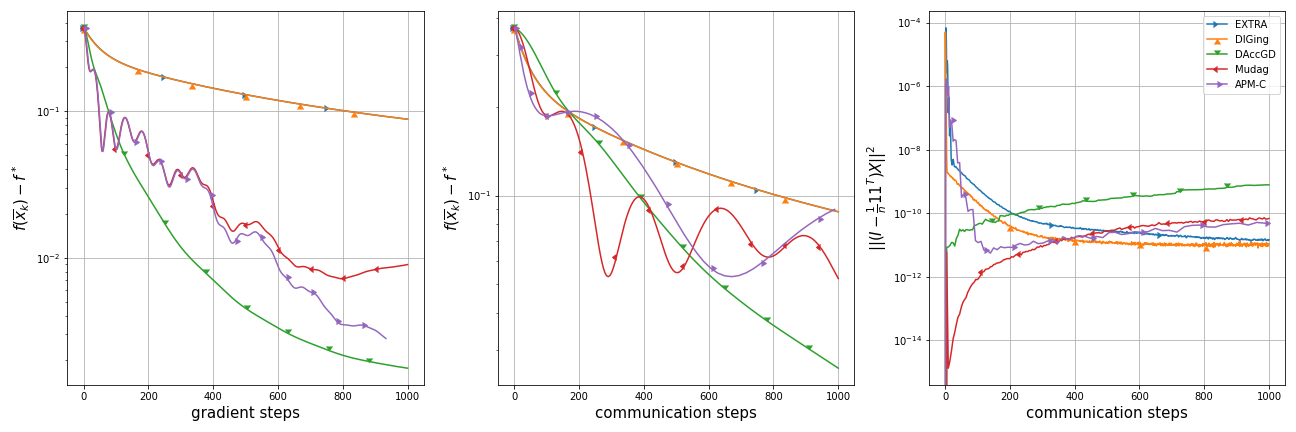
Figure 1: a9a (logistic regression), $100$ nodes

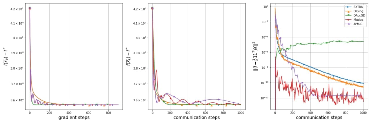
Figure 2: cadata (least squares), $20$ nodes

5 Conclusion

This paper studies an inexact oracle-based approach to decentralized optimization. The paper focuses on a specific case of strongly convex smooth functions, but the inexact oracle framework introduced in [3] is also applicable to non-strongly convex functions. The development of this framework in [28] also enables to generalize the results of this article to composite optimization problems and distributed algorithms for saddle-point problems and variational inequalities.

Another interesting application of inexact oracle approach lies in stochastic decentralized algorithms. Consider a class of $L$-smooth $\mu$-strongly convex objectives with gradient noise of each $f_{i}$ being upper-bounded by $\sigma^{2}$. For this class of problems, lower complexity bounds write as [32]

$$O(\sqrt{L/\mu\chi}\log(1/\varepsilon))$$ stochastic oracle calls per node

$$O\left(\max\left(\frac{\sigma^{2}}{m\mu\varepsilon},\sqrt{L/\mu}\right)\log(1/\varepsilon)\right) \qquad\text{communication steps}.$$

At the moment, there exist methods which are optimal either in the number of oracle calls or in the number of communication steps. We believe that approach of this paper combined with a specific batch-size choice described in [33] allows to develop a decentralized algorithm reaching both optimal complexities.

6 Acknowledgements

The authors are grateful to Dmitriy Metelev and Fedor Stonyakin for their thoughtful proofreading of the paper.

Appendix A Proof of Theorem 3.3

A.1 Gradient step

Consider update rule

$$Y=\operatorname*{arg\,min}_{X\in\mathbb{R}^{n\times d}}\left\{\left\langle P,X\right\rangle+\frac{1}{2}\left\|X\right\|^{2}\right\},\text{ where }P=\begin{pmatrix}p_{1}^{\top}\\ \vdots\\ p_{n}^{\top}\end{pmatrix}\in\mathbb{R}^{n\times d}.$$ (14)

By first-order optimality conditions $Y=-P$. Therefore $\overline{y}=-\overline{p}$ and

$$\overline{y}=\operatorname*{arg\,min}_{x\in\mathbb{R}^{d}}\left\{\left\langle\overline{p},x\right\rangle+\frac{1}{2}\left\|x\right\|^{2}\right\}.$$ (15)

This means that update rule (14) in $\mathbb{R}^{n\times d}$ comes down to update rule (15) in $\mathbb{R}^{d}$. In the case of gradient step, $P=\frac{1}{L}\nabla F(X^{k})-X^{k}$, and step

$$X^{k+1}=X^{k}-\frac{1}{L}\nabla F(X^{k})$$

is comes down to $x^{k+1}=x^{k}-\frac{1}{L}\left(\frac{1}{n}\sum_{i=1}^{n}\nabla f_{i}(x_{i})\right)$.

Since update rule 5 in Algorithm 1 has form (14), Algorithm 1 comes down to an iterative procedure in $\mathbb{R}^{d}$.

$$\overline{y}^{k+1} =\frac{\alpha^{k+1}\overline{u}^{k}+A^{k}\overline{x}^{k}}{A^{k+1}}$$

$$\overline{u}^{k+1} =\operatorname*{arg\,min}_{\overline{z}\in\mathbb{R}^{d}}\left\{\alpha^{k+1}\left(\left\langle\frac{1}{n}\sum_{i=1}^{n}\nabla f(y_{i}^{k+1}),\overline{z}-\overline{y}^{k+1}\right\rangle+\frac{\mu}{2}\left\|\overline{z}-\overline{y}^{k+1}\right\|^{2}\right)+\frac{1+A^{k}\mu}{2}\left\|\overline{z}-\overline{u}^{k}\right\|^{2}\right\}$$

$$\overline{x}^{k+1} =\frac{\alpha^{k+1}\overline{u}^{k+1}+A^{k}\overline{x}^{k}}{A^{k+1}}$$

A.2 Outer loop

Initially we recall basic properties of coefficients $A^{k}$.

Lemma A.1.

For coefficients $A^{k}$, it holds

$$1.\leavevmode\nobreak\ A^{N}\geqslant\frac{1}{L}\left(1+\frac{1}{2}\sqrt{\frac{\mu}{L}}\right)^{2(N-1)}$$

$$2.\leavevmode\nobreak\ \frac{\sum_{i=1}^{k}A^{i}}{A^{k}}\leqslant{1+\sqrt{\frac{L}{\mu}}}.$$

Proof.

For first statement see [28], Lemma 3.7.

Recall update rule for $A^{k}$:

$$1+\mu A^{k}=\frac{L(\alpha^{k+1})^{2}}{A^{k+1}},\leavevmode\nobreak\ A^{k}=\sum_{i=0}^{k}\alpha^{i},\leavevmode\nobreak\ \alpha^{0}=0.$$ (16)

In [4] an almost similar sequence is studied:

$$L+\mu B^{k}=\frac{L(\beta^{k+1})^{2}}{B^{k+1}},\leavevmode\nobreak\ B^{k}=\sum_{i=0}^{k}\beta^{i},\leavevmode\nobreak\ \beta^{0}=1,$$ (17)

and for sequence $\left\{B^{k}\right\}_{k=0}^{\infty}$ it is shown $\frac{\sum_{i=0}^{k}B^{i}}{B^{k}}\leqslant 1+\sqrt{L/\mu}$. Dividing (17) by L yields

$$1+\mu(B^{k}/L)=\frac{L(\beta^{k+1}/L)^{2}}{(B^{k+1}/L)},$$

which means that update rule for $B^{k}/L$ is equivalent to (16). Since $A^{1}=1/L=B^{0}/L$, it holds $A^{k+1}=B^{k}/L,\leavevmode\nobreak\ k\geqslant 0$ and

$$\frac{\sum_{i=1}^{k}A^{i}}{A^{k}}=\frac{\sum_{i=0}^{k-1}B^{i}/L}{B^{k-1}/L}\leqslant 1+\sqrt{\frac{L}{\mu}}.$$

∎

Lemma A.2.

Provided that consensus accuracy is $\delta^{\prime}$, i.e. $\left\|{\bf U}^{j}-\overline{\bf U}^{j}\right\|^{2}\leqslant\delta^{\prime}\text{ for }j=1,\ldots,k$, we have

$$f(\overline{x}^{k})-f(x^{*}) \leqslant\frac{\left\|\overline{u}^{0}-x^{*}\right\|^{2}}{2A^{k}}+\frac{2\sum_{j=1}^{k}A^{j}\delta}{A^{k}}$$

$$\left\|\overline{u}^{k}-x^{*}\right\|^{2} \leqslant\frac{\left\|\overline{u}^{0}-x^{*}\right\|^{2}}{1+A^{k}\mu}+\frac{4\sum_{j=1}^{k}A^{j}\delta}{1+A^{k}\mu}$$

where $\delta$ is given in (5).

Proof.

First, assuming that $\left\|{\bf U}^{j}-\overline{\bf U}^{j}\right\|^{2}\leqslant\delta^{\prime}$, we show that ${\bf Y}^{j},{\bf U}^{j},{\bf X}^{j}$ lie in $\sqrt{\delta^{\prime}}$-neighborhood of $\mathcal{C}$ by induction. At $j=0$, we have $\left\|{\bf X}^{0}-\overline{\bf X}^{0}\right\|=\left\|{\bf U}^{0}-\overline{\bf U}^{0}\right\|=0$. Using $A^{j+1}=A^{j}+\alpha^{j}$, we get an induction pass $j\to j+1$.

$$\left\|{\bf Y}^{j+1}-\overline{\bf Y}^{j+1}\right\| \leqslant\frac{\alpha^{j+1}}{A^{j+1}}\left\|{\bf U}^{j}-\overline{\bf U}^{j}\right\|+\frac{A^{j}}{A^{j+1}}\left\|{\bf X}^{j}-\overline{\bf X}^{j}\right\|\leqslant\sqrt{\delta^{\prime}}$$

$$\left\|{\bf X}^{j+1}-\overline{\bf X}^{j+1}\right\| \leqslant\frac{\alpha^{j+1}}{A^{j+1}}\left\|{\bf U}^{j+1}-\overline{\bf U}^{j+1}\right\|+\frac{A^{j}}{A^{j+1}}\left\|{\bf X}^{j}-\overline{\bf X}^{j}\right\|\leqslant\sqrt{\delta^{\prime}}$$

Therefore, $g(\overline{y})=\frac{1}{n}\sum_{i=1}^{n}\nabla f(y_{i})$ is a gradient from $(\delta,L,\mu)$-model of $f$, and the desired result directly follows from Theorem 3.4 in [28]. ∎

A.3 Consensus subroutine iterations

How many consensus iterations we need to reach accuracy $\delta^{\prime}$? We formulate the corresponding result in the following

Lemma A.3.

Let consensus accuracy be maintained at level $\delta^{\prime}$, i.e. $\left\|{\bf U}^{j}-\overline{\bf U}^{j}\right\|^{2}\leqslant\delta^{\prime}\text{ for }j=1,\ldots,k$ and let Assumption 3.1 hold. Define

$$\sqrt{D}:=\left(\frac{2L_{l}}{\sqrt{L\mu}}+1\right)\sqrt{\delta^{\prime}}+\frac{L_{l}}{\mu}\sqrt{n}\left(\left\|\overline{u}^{0}-x^{*}\right\|^{2}+\frac{8{\delta^{\prime}}}{\sqrt{L\mu}}\right)^{1/2}+\frac{2\left\|\nabla F({\bf X}^{*})\right\|}{\sqrt{L\mu}}$$

Then it is sufficient to make $T_{k}=T=\frac{\tau}{2\lambda}\log\frac{D}{\delta^{\prime}}$ consensus iterations in order to ensure $\delta^{\prime}$-accuracy on step $k+1$, i.e. $\left\|{\bf U}^{k+1}-\overline{\bf U}^{k+1}\right\|^{2}\leqslant\delta^{\prime}$.

Proof.

First, note that multiplication by mixing matrix preserves average, i.e. $\frac{1}{n}\mathbf{1}_{n}\mathbf{1}_{n}^{\top}{\bf X}=\frac{1}{n}\mathbf{1}_{n}\mathbf{1}_{n}^{\top}{\bf W}^{k}{\bf X}\leavevmode\nobreak\ \forall k\geqslant 0$. In particular, this implies $\overline{\bf U}^{k+1}=\overline{\bf V}^{k+1}$.

By contraction property of mixing matrix sequence $\{{\bf W}^{k}\}_{k=0}^{\infty}$ it holds

$$\left\|{\bf U}^{k+1}-\overline{\bf U}^{k+1}\right\|^{2}\leqslant(1-\lambda)^{2(T/\tau)}\left\|{\bf V}^{k+1}-\overline{\bf U}^{k+1}\right\|^{2}\leqslant e^{-2(T/\tau)\lambda}\left\|{\bf V}^{k+1}-\overline{\bf U}^{k+1}\right\|^{2}$$

Assuming that $\left\|{\bf V}^{k+1}-\overline{\bf U}^{k+1}\right\|^{2}\leqslant D$, we only need $T=\frac{\tau}{2\lambda}\log\frac{D}{\delta^{\prime}}$ iterations to ensure $\left\|{\bf U}^{k+1}-\overline{\bf U}^{k+1}\right\|^{2}\leqslant\delta^{\prime}$. In the rest of the proof, we show that $\left\|{\bf V}^{k+1}-\overline{\bf U}^{k+1}\right\|=\left\|{\bf V}^{k+1}-\overline{\bf V}^{k+1}\right\|\leqslant\sqrt{D}$.

From optimality conditions for update rule (5) of Algorithm 1 it holds

$${\bf V}^{k+1}=\frac{\alpha^{k+1}\mu{\bf Y}^{k+1}+(1+A^{k}\mu){\bf U}^{k}}{1+A^{k+1}\mu}-\frac{\alpha^{k+1}}{1+A^{k+1}\mu}\nabla F({\bf Y}^{k+1})$$

and thus

$$\left\|{\bf V}^{k+1}-\overline{\bf V}^{k+1}\right\| \leqslant\frac{\alpha^{k+1}\mu\left\|{\bf Y}^{k+1}-\overline{\bf Y}^{k+1}\right\|}{1+A^{k+1}\mu}+\frac{(1+A^{k}\mu)\left\|{\bf U}^{k}-\overline{\bf U}^{k}\right\|}{1+A^{k+1}\mu}+\frac{\alpha^{k+1}}{1+A^{k+1}\mu}\left\|\nabla F({\bf Y}^{k+1})\right\|$$

$$\leqslant\sqrt{\delta^{\prime}}+\frac{\alpha^{k+1}}{1+A^{k+1}\mu}\left\|\nabla F({\bf Y}^{k+1})\right\|.$$

We estimate $\left\|\nabla F({\bf Y}^{k+1})\right\|$ using $L_{l}$-smoothness of $F$:

$$\left\|\nabla F({\bf Y}^{k+1})\right\| \leqslant\left\|\nabla F({\bf Y}^{k+1})-\nabla F({\bf X}^{*})\right\|+\left\|\nabla F({\bf X}^{*})\right\|$$

$$\leqslant L_{l}\underbrace{\left\|{\bf Y}^{k+1}-\overline{\bf Y}^{k+1}\right\|}_{\leqslant\sqrt{\delta^{\prime}}}+L_{l}\underbrace{\left\|\overline{\bf Y}^{k+1}-{\bf X}^{*}\right\|}_{=\sqrt{n}\left\|\overline{y}^{k+1}-x^{*}\right\|}+\left\|\nabla F({\bf X}^{*})\right\|$$ (18)

where

$${\bf X}^{*}=\begin{pmatrix}(x^{*})^{\top}\\ \vdots\\ (x^{*})^{\top}\end{pmatrix},\leavevmode\nobreak\ x^{*}=\operatorname*{arg\,min}_{x\in\mathbb{R}^{d}}f(x).$$

It remains to estimate $\left\|\overline{y}^{k+1}-x^{*}\right\|$.

$$\left\|\overline{y}^{k+1}-x^{*}\right\| \leqslant\frac{\alpha^{k+1}}{A^{k+1}}\left\|\overline{x}^{k+1}-x^{*}\right\|+\frac{A^{k}}{A^{k+1}}\left\|\overline{u}^{k+1}-x^{*}\right\|\leqslant\max\left\{\left\|\overline{x}^{k+1}-x^{*}\right\|,\left\|\overline{u}^{k+1}-x^{*}\right\|\right\}$$

By Lemma A.2 and strong convexity of $f$:

$$\left\|\overline{x}^{k+1}-x^{*}\right\|^{2}\leqslant\frac{2}{\mu}\left(f(\overline{x}^{k+1})-f(x^{*})\right)\leqslant\frac{\left\|\overline{u}^{0}-x^{*}\right\|^{2}}{A^{k+1}\mu}+\frac{4\sum_{i=1}^{k+1}A^{i}\delta^{\prime}}{A^{k+1}\mu}$$

and therefore

$$\left\|\overline{y}^{k+1}-x^{*}\right\|^{2} \leqslant\max\left\{\frac{\left\|\overline{u}^{0}-x^{*}\right\|^{2}}{A^{k+1}\mu}+\frac{4\sum_{i=1}^{k+1}A^{i}\delta^{\prime}}{A^{k+1}\mu},\leavevmode\nobreak\ \frac{\left\|\overline{u}^{0}-x^{*}\right\|^{2}}{1+A^{k+1}\mu}+\frac{4\sum_{i=1}^{k+1}A^{i}\delta^{\prime}}{1+A^{k+1}\mu}\right\}$$

$$\overset{\text{\char 172}}{\leqslant}\frac{\left\|\overline{u}^{0}-x^{*}\right\|^{2}}{A^{k+1}\mu}+\frac{4}{\mu}\left(1+\sqrt{\frac{L}{\mu}}\right)\delta^{\prime},$$

where the last inequality holds by Lemma A.1.

Returning to (18), we get

$$\left\|\nabla F({\bf Y}^{k+1})\right\| \leqslant L_{l}\sqrt{\delta^{\prime}}+L_{l}\sqrt{n}\left(\frac{\left\|\overline{u}^{0}-x^{*}\right\|^{2}}{A^{k+1}\mu}+\frac{4}{\mu}\left(1+\sqrt{\frac{L}{\mu}}\right)\delta^{\prime}\right)^{1/2}+\left\|\nabla F({\bf X}^{*})\right\|$$

$$\leqslant L_{l}\sqrt{\delta^{\prime}}+L_{l}\sqrt{n}\left(\frac{L}{\mu}\left\|\overline{u}^{0}-x^{*}\right\|^{2}\left(1+\frac{1}{2}\sqrt{\frac{\mu}{L}}\right)^{-2k}+\frac{8L^{1/2}}{\mu^{3/2}}\delta^{\prime}\right)^{1/2}+\left\|\nabla F({\bf X}^{*})\right\|$$

$$\leqslant L_{l}\sqrt{\delta^{\prime}}+L_{l}\sqrt{n}\left(\frac{L}{\mu}\left\|\overline{u}^{0}-x^{*}\right\|^{2}+\frac{8L^{1/2}}{\mu^{3/2}}{\delta^{\prime}}\right)^{1/2}+\left\|\nabla F({\bf X}^{*})\right\|.$$

For distance to consensus of ${\bf V}^{k+1}$, it holds

$$\left\|{\bf V}^{k+1}-\overline{\bf V}^{k+1}\right\|\leqslant\sqrt{\delta^{\prime}}+\frac{\alpha^{k+1}}{1+A^{k+1}\mu}\left\|\nabla F\left({\bf Y}^{k+1}\right)\right\|$$

We estimate coefficient by $\left\|\nabla F\left({\bf Y}^{k+1}\right)\right\|$ using the definition of $\alpha^{k+1}$.

$$1+A^{k}\mu=\frac{L(\alpha^{k+1})^{2}}{A^{k}+\alpha^{k+1}}$$

$$L(\alpha^{k+1})^{2}-(1+A^{k}\mu)\alpha^{k+1}-(1+A^{k}\mu)A^{k}=0$$

$$\alpha^{k+1}=\frac{1+A^{k}\mu+\sqrt{(1+A^{k}\mu)^{2}+4LA^{k}(1+A^{k}\mu)}}{2L}$$

$$\frac{\alpha^{k+1}}{1+A^{k+1}\mu}\leqslant\frac{\alpha^{k+1}}{1+A^{k}\mu}=\frac{1}{2L}\left(1+\sqrt{1+4\frac{LA^{k}}{1+A^{k}\mu}}\right)$$

$$\qquad\leqslant\frac{1}{2L}\left(\sqrt{\frac{L}{\mu}}+\sqrt{\frac{L}{\mu}+4\frac{L}{\mu}}\right)\leqslant\frac{2}{\sqrt{L\mu}}$$

Returning to ${\bf V}^{k+1}$, we get

$$\left\|{\bf V}^{k+1}-\overline{\bf V}^{k+1}\right\| \leqslant\left(\frac{2L_{l}}{\sqrt{L\mu}}+1\right)\sqrt{\delta^{\prime}}+L_{l}\sqrt{\frac{n}{L\mu}}\left(\frac{L}{\mu}\left\|\overline{u}^{0}-x^{*}\right\|^{2}+\frac{8L^{1/2}}{\mu^{3/2}}{\delta^{\prime}}\right)^{1/2}+\frac{2\left\|\nabla F({\bf X}^{*})\right\|}{\sqrt{L\mu}}$$

$$=\left(\frac{2L_{l}}{\sqrt{L\mu}}+1\right)\sqrt{\delta^{\prime}}+\frac{L_{l}}{\mu}\sqrt{n}\left(\left\|\overline{u}^{0}-x^{*}\right\|^{2}+\frac{8{\delta^{\prime}}}{\sqrt{L\mu}}\right)^{1/2}+\frac{2\left\|\nabla F({\bf X}^{*})\right\|}{\sqrt{L\mu}}=\sqrt{D}$$

which concludes the proof. ∎

A.4 Putting the proof together

Let us show that choice of number of subroutine iterations $T_{k}=T$ yields

$$f(\overline{x}^{k})-f(x^{*})\leqslant\frac{\left\|\overline{u}^{0}-x^{*}\right\|^{2}}{2A^{k}}+\frac{2\sum_{j=1}^{k}A^{j}\delta}{A^{k}}$$

by induction. At $k=0$, we have $\left\|{\bf U}^{0}-\overline{\bf U}^{0}\right\|=0$ and by Lemma A.2 it holds

$$f(\overline{x}^{1})-f(x^{*})\leqslant\frac{\left\|\overline{u}^{0}-x^{*}\right\|^{2}}{2A^{1}}+\frac{2A^{1}\delta}{A^{1}}.$$

For induction pass, assume that $\left\|{\bf U}^{j}-\overline{\bf U}^{j}\right\|^{2}\leqslant\delta^{\prime}$ for $j=0,\ldots,k$. By Lemma A.3, if we set $T_{k}=T$, then $\left\|{\bf U}^{k+1}-\overline{\bf U}^{k+1}\right\|^{2}\leqslant\delta^{\prime}$. Applying Lemma A.2 again, we get

$$f(\overline{x}^{k+1})-f(x^{*})\leqslant\frac{\left\|\overline{u}^{0}-x^{*}\right\|^{2}}{2A^{k+1}}+\frac{2\sum_{j=1}^{k+1}A^{j}\delta}{A^{k+1}}$$

Recalling a bound on $A^{k}$ from Lemma A.1 gives

$$f(\overline{x}^{N})-f(x^{*}) \leqslant\frac{L\left\|\overline{u}^{0}-x^{*}\right\|^{2}}{2}\left(1+\frac{1}{2}\sqrt{\frac{\mu}{L}}\right)^{-2(N-1)}+2\left(1+\sqrt{\frac{L}{\mu}}\right)\delta$$

$$\overset{\text{\char 172}}{=}L_{g}\left\|\overline{u}^{0}-x^{*}\right\|^{2}\left(1+\frac{1}{4}\sqrt{\frac{\mu_{g}}{L_{g}}}\right)^{-2(N-1)}+2\left(1+2\sqrt{\frac{L_{g}}{\mu_{g}}}\right)\delta$$

Here in ① we used the definition of $L,\mu$ in (10): $L=2L_{g},\leavevmode\nobreak\ \mu=\frac{\mu_{g}}{2}$. For $\varepsilon$-accuracy:

$$L_{g}\left\|\overline{u}^{0}-x^{*}\right\|^{2}\left(1+\frac{1}{4}\sqrt{\frac{\mu_{g}}{L_{g}}}\right)^{-2(N-1)}\leqslant\frac{\varepsilon}{2}\longrightarrow\leavevmode\nobreak\ N\geqslant 1+\sqrt{\frac{L_{g}}{\mu_{g}}}\log\left(\frac{2L_{g}\left\|\overline{u}^{0}-x^{*}\right\|^{2}}{\varepsilon}\right)$$

$$2\left(1+2\sqrt{\frac{L_{g}}{\mu_{g}}}\right)\delta\leqslant\frac{\varepsilon}{2}\longrightarrow\leavevmode\nobreak\ \delta^{\prime}\leqslant\frac{n\varepsilon}{2}\left(1+2\sqrt{\frac{L_{g}}{\mu_{g}}}\right)^{-1}\left(L_{l}^{2}\left(\frac{1}{L_{g}}+\frac{2}{\mu_{g}}\right)+L_{l}-\mu_{l}\right)^{-1}$$

It is sufficient to choose

$$N=2\sqrt{\frac{L_{g}}{\mu_{g}}}\log\left(\frac{2L_{g}\left\|\overline{u}^{0}-x^{*}\right\|^{2}}{\varepsilon}\right)$$

$$\delta^{\prime}=\frac{n\varepsilon}{2}\cdot\frac{1}{2}\cdot\frac{1}{2}\sqrt{\frac{\mu_{g}}{L_{g}}}\cdot\left(4\frac{L_{l}^{2}}{\mu_{g}}\right)^{-1}=\frac{n\varepsilon}{32}\frac{\mu_{g}^{3/2}}{L_{g}^{1/2}L_{l}^{2}}$$

Let us estimate the term $\frac{D}{\delta^{\prime}}$ under $\log$.

$$\sqrt{\frac{D}{\delta^{\prime}}} =\left(\frac{2L_{l}}{\sqrt{L\mu}}+1\right)+\frac{L_{l}}{\mu}\sqrt{n}\left(\frac{\left\|\overline{u}^{0}-x^{*}\right\|^{2}}{\delta^{\prime}}+\frac{8}{\sqrt{L\mu}}\right)^{1/2}+\frac{2\left\|\nabla F({\bf X}^{*})\right\|}{\sqrt{L\mu}\sqrt{\delta^{\prime}}}$$

$$\leqslant\frac{3L_{l}}{\sqrt{L_{g}\mu_{g}}}+\frac{2L_{l}\sqrt{n}}{\mu_{g}}\left(\sqrt{\frac{\left\|\overline{u}^{0}-x^{*}\right\|^{2}}{n\varepsilon}\cdot\frac{32L_{g}^{1/2}L_{l}^{2}}{\mu_{g}^{3/2}}}+\sqrt{\frac{8}{\sqrt{L_{g}\mu_{g}}}}\right)+\frac{2\left\|\nabla F({\bf X}^{*})\right\|}{\sqrt{L_{g}\mu_{g}}}\cdot\frac{\sqrt{32}}{\sqrt{n\varepsilon}}\frac{L_{g}^{1/4}L_{l}}{\mu_{g}^{3/4}}$$

$$=\frac{3L_{l}}{\sqrt{L_{g}\mu_{g}}}+\frac{8\sqrt{2}L_{l}^{2}L_{g}^{1/4}\left\|\overline{u}^{0}-x^{*}\right\|}{\mu_{g}^{7/4}\sqrt{\varepsilon}}+\frac{4\sqrt{2}L_{l}\sqrt{n}}{L_{g}^{1/4}\mu_{g}^{5/4}}+\frac{4\sqrt{2}\left\|\nabla F({\bf X}^{*})\right\|\cdot L_{l}}{L_{g}^{1/4}\mu_{g}^{5/4}\sqrt{n\varepsilon}}$$

$$=\frac{L_{l}}{L_{g}^{1/2}\mu_{g}}\left[3\sqrt{\mu}_{g}+\frac{8\sqrt{2}L_{l}\left\|\overline{u}^{0}-x^{*}\right\|}{\sqrt{\varepsilon}}\left(\frac{L_{g}}{\mu_{g}}\right)^{3/4}+4\sqrt{2n}\left(\frac{L_{g}}{\mu_{g}}\right)^{1/4}+\frac{4\sqrt{2}\left\|\nabla F({\bf X}^{*})\right\|}{\sqrt{n\varepsilon}}\left(\frac{L_{g}}{\mu_{g}}\right)^{1/4}\right]$$

$$=\frac{D_{1}}{\sqrt{\varepsilon}}+D_{2},$$

where $D_{1},D_{2}$ are defined in (11). Finally, the total number of iterations is

$$N_{\text{tot}} =N\cdot T=2\sqrt{\frac{L_{g}}{\mu_{g}}}\log\left(\frac{2L_{g}\left\|\overline{u}^{0}-x^{*}\right\|^{2}}{\varepsilon}\right)\cdot\frac{\tau}{2\lambda}\cdot 2\log\sqrt{\frac{D}{\delta^{\prime}}}$$

$$=2\sqrt{\frac{L_{g}}{\mu_{g}}}\frac{\tau}{\lambda}\cdot\log\left(\frac{2L_{g}\left\|\overline{u}^{0}-x^{*}\right\|^{2}}{\varepsilon}\right)\log\left(\frac{D_{1}}{\sqrt{\varepsilon}}+D_{2}\right).$$

References

• [1] Angelia Nediฤ‡, Alex Olshevsky, and Cรฉsarย A Uribe. Fast convergence rates for distributed non-bayesian learning. IEEE Transactions on Automatic Control, 62(11):5538โ€“5553, 2017.
• [2] Sundharย Srinivasan Ram, Venugopalย V Veeravalli, and Angelia Nedic. Distributed non-autonomous power control through distributed convex optimization. In IEEE INFOCOM 2009, pages 3001โ€“3005. IEEE, 2009.
• [3] Olivier Devolder, Franรงois Glineur, and Yurii Nesterov. First-order methods of smooth convex optimization with inexact oracle. Mathematical Programming, 146(1-2):37โ€“75, 2014.
• [4] O.ย Devolder, F.ย Glineur, and Yu. Nesterov. First-order methods with inexact oracle: the strongly convex case. CORE Discussion Papers, 2013016:47, 2013.
• [5] Duลกan Jakovetiฤ‡, Joao Xavier, and Josรฉย MF Moura. Fast distributed gradient methods. IEEE Transactions on Automatic Control, 59(5):1131โ€“1146, 2014.
• [6] Angelia Nediฤ‡, Alex Olshevsky, and Wei Shi. Achieving geometric convergence for distributed optimization over time-varying graphs. SIAM Journal on Optimization, 27(4):2597โ€“2633, 2017.
• [7] Kevin Scaman, Francis Bach, Sรฉbastien Bubeck, Laurent Massouliรฉ, and Yinย Tat Lee. Optimal algorithms for non-smooth distributed optimization in networks. In Advances in Neural Information Processing Systems, pages 2740โ€“2749, 2018.
• [8] Shi Pu, Wei Shi, Jinming Xu, and Angelia Nedich. A push-pull gradient method for distributed optimization in networks. 2018 IEEE Conference on Decision and Control (CDC), pages 3385โ€“3390, 2018.
• [9] G.ย Qu and N.ย Li. Accelerated distributed nesterov gradient descent. 2016 54th Annual Allerton Conference on Communication, Control, and Computing, 2016.
• [10] Wei Shi, Qing Ling, Gang Wu, and Wotao Yin. Extra: An exact first-order algorithm for decentralized consensus optimization. SIAM Journal on Optimization, 25(2):944โ€“966, 2015.
• [11] Haishan Ye, Luo Luo, Ziang Zhou, and Tong Zhang. Multi-consensus decentralized accelerated gradient descent. arXiv preprint arXiv:2005.00797, 2020.
• [12] Huan Li, Cong Fang, Wotao Yin, and Zhouchen Lin. A sharp convergence rate analysis for distributed accelerated gradient methods. arXiv:1810.01053, 2018.
• [13] Angelia Nedic and Asuman Ozdaglar. Distributed subgradient methods for multi-agent optimization. IEEE Transactions on Automatic Control, 54(1):48โ€“61, 2009.
• [14] Kevin Scaman, Francis Bach, Sรฉbastien Bubeck, Yinย Tat Lee, and Laurent Massouliรฉ. Optimal algorithms for smooth and strongly convex distributed optimization in networks. In International Conference on Machine Learning, pages 3027โ€“3036, 2017.
• [15] D.ย Jakovetic. A unification and generalization of exact distributed first order methods. IEEE Transactions on Signal and Information Processing over Networks, pages 31โ€“46, 2019.
• [16] Alexander Rogozin and Alexander Gasnikov. Projected gradient method for decentralized optimization over time-varying networks. arXiv preprint arXiv:1911.08527, 2019.
• [17] Darina Dvinskikh and Alexander Gasnikov. Decentralized and parallelized primal and dual accelerated methods for stochastic convex programming problems. arXiv preprint arXiv:1904.09015, 2019.
• [18] Huan Li and Zhouchen Lin. Revisiting extra for smooth distributed optimization. arXiv preprint arXiv:2002.10110, 2020.
• [19] Hadrien Hendrikx, Francis Bach, and Laurent Massoulie. An optimal algorithm for decentralized finite sum optimization. arXiv preprint arXiv:2005.10675, 2020.
• [20] Huan Li, Zhouchen Lin, and Yongchun Fang. Optimal accelerated variance reduced extra and diging for strongly convex and smooth decentralized optimization. arXiv preprint arXiv:2009.04373, 2020.
• [21] X.ย Wu and J.ย Lu. Fenchel dual gradient methods for distributed convex optimization over time-varying networks. In 2017 IEEE 56th Annual Conference on Decision and Control (CDC), pages 2894โ€“2899, Dec 2017.
• [22] G.ย Zhang and R.ย Heusdens. Distributed optimization using the primal-dual method of multipliers. IEEE Transactions on Signal and Information Processing over Networks, 4(1):173โ€“187, 2018.
• [23] Cรฉsarย A Uribe, Soomin Lee, Alexander Gasnikov, and Angelia Nediฤ‡. A dual approach for optimal algorithms in distributed optimization over networks. Optimization Methods and Software, pages 1โ€“40, 2020.
• [24] Yossi Arjevani, Joan Bruna, Bugra Can, Mert Gรผrbรผzbalaban, Stefanie Jegelka, and Hongzhou Lin. Ideal: Inexact decentralized accelerated augmented lagrangian method. arXiv preprint arXiv:2006.06733, 2020.
• [25] Ermin Wei and Asuman Ozdaglar. Distributed alternating direction method of multipliers. In 2012 IEEE 51st IEEE Conference on Decision and Control (CDC), pages 5445โ€“5450. IEEE, 2012.
• [26] Marie Maros and Joakim Jaldรฉn. Panda: A dual linearly converging method for distributed optimization over time-varying undirected graphs. 2018 IEEE Conference on Decision and Control (CDC), pages 6520โ€“6525, 2018.
• [27] Junqi Tang, Karen Egiazarian, Mohammad Golbabaee, and Mike Davies. The practicality of stochastic optimization in imaging inverse problems. arXiv preprint arXiv:1910.10100, 2019.
• [28] F.ย Stonyakin, A.ย Tyurin, A.ย Gasnikov, P.ย Dvurechensky, A.ย Agafonov, D.ย Dvinskikh, D.ย Pasechnyuk, S.ย Artamonov, and V.ย Piskunova. Inexact relative smoothness and strong convexity for optimization and variational inequalities by inexact model. arXiv:2001.09013, 2020.
• [29] Anastasia Koloskova, Nicolas Loizou, Sadra Boreiri, Martin Jaggi, and Sebastianย U Stich. A unified theory of decentralized sgd with changing topology and local updates. arXiv preprint arXiv:2003.10422, 2020.
• [30] Chih-Chung Chang and Chih-Jen Lin. Libsvm: a library for support vector machines. ACM transactions on intelligent systems and technology (TIST), 2(3):27, 2011.
• [31] Huan Li, Cong Fang, Wotao Yin, and Zhouchen Lin. Decentralized accelerated gradient methods with increasing penalty parameters. IEEE Transactions on Signal Processing, 68:4855โ€“4870, 2020.
• [32] Yossi Arjevani and Ohad Shamir. Communication complexity of distributed convex learning and optimization. Advances in neural information processing systems, 28:1756โ€“1764, 2015.
• [33] Darinaย M Dvinskikh, Aleksandrย Igorevich Turin, Alexanderย Vladimirovich Gasnikov, and Sergeyย Sergeevich Omelchenko. Accelerated and non accelerated stochastic gradient descent in model generality. Matematicheskie Zametki, 108(4):515โ€“528, 2020.