The Atacama Cosmology Telescope: A Catalog of $>4000$ Sunyaev-Zel’dovich Galaxy Clusters

Abstract

We present a catalog of 4195 optically confirmed Sunyaev-Zel’dovich (SZ) selected galaxy clusters detected with signal-to-noise $>4$ in 13,211 deg² of sky surveyed by the Atacama Cosmology Telescope (ACT). Cluster candidates were selected by applying a multi-frequency matched filter to 98 and 150 GHz maps constructed from ACT observations obtained from 2008–2018, and confirmed using deep, wide-area optical surveys. The clusters span the redshift range $0.04{}<z<1.91{}$ (median $z=0.52{}$). The catalog contains 222 $z>1$ clusters, and a total of 868 systems are new discoveries. Assuming an SZ-signal vs. mass scaling relation calibrated from X-ray observations, the sample has a 90% completeness mass limit of $M_{\rm 500c}>3.8{}\times 10^{14}$ $M_{\sun}$, evaluated at $z=0.5$, for clusters detected at signal-to-noise ratio $>5$ in maps filtered at an angular scale of 2.4′. The survey has a large overlap with deep optical weak-lensing surveys that are being used to calibrate the SZ-signal mass-scaling relation, such as the Dark Energy Survey (4566 deg²), the Hyper Suprime-Cam Subaru Strategic Program (469 deg²), and the Kilo Degree Survey (825 deg²). We highlight some noteworthy objects in the sample, including potentially projected systems; clusters with strong lensing features; clusters with active central galaxies or star formation; and systems of multiple clusters that may be physically associated. The cluster catalog will be a useful resource for future cosmological analyses, and studying the evolution of the intracluster medium and galaxies in massive clusters over the past 10 Gyr.

DES-2020-0547 FERMILAB-PUB-20-458-AE

1 Introduction

The thermal Sunyaev-Zel’dovich effect (SZ; e.g., Sunyaev & Zel’dovich, 1970; Sunyaev & Zeldovich, 1972) is well established as a method for constructing approximately mass-limited samples of galaxy clusters, independently of redshift. The SZ effect arises through the inverse Compton scattering of cosmic microwave background (CMB) photons by electrons within the hot gas atmospheres of galaxy clusters (see reviews by Birkinshaw, 1999; Carlstrom et al., 2002; Mroczkowski et al., 2019). This leads to a spectral distortion in sight lines towards clusters, such that at frequencies below 220 GHz, clusters appear as “cold spots” in the mm-wave sky, while at frequencies above 220 GHz, they appear as “hot spots.” The amplitude of the SZ signal scales with the mass of the cluster.

The unique power of SZ-selected cluster surveys to detect all of the massive structures in the Universe regardless of their distance from the observer has driven the development of “blind” SZ surveys that constrain cosmological parameters through measuring the evolution of the cluster mass function (e.g., Vanderlinde et al., 2010; Sehgal et al., 2011; Hasselfield et al., 2013; Reichardt et al., 2013; Planck Collaboration et al., 2014a, 2016a; Bocquet et al., 2019). SZ cluster surveys over large areas of sky have been conducted by the South Pole Telescope (SPT; e.g., Williamson et al., 2011; Bleem et al., 2015b, 2020; Huang et al., 2020a), the Planck satellite mission (Planck Collaboration et al., 2014b, 2016b), and the Atacama Cosmology Telescope (ACT; Marriage et al., 2011; Hasselfield et al., 2013; Hilton et al., 2018). Collectively, since the first blind SZ detections by SPT (Staniszewski et al., 2009), these surveys have detected approximately 2300 clusters with redshift measurements to date.

In this paper we present the first cluster catalog derived from observations using the Advanced ACTPol receiver (Henderson et al., 2016; Ho et al., 2017; Choi et al., 2018), combining this with all observations by ACT from 2008–2018 (Naess et al. 2020, N20 hereafter; details of previous generations of ACT instrumentation can be found in Fowler et al. 2007, Swetz et al. 2011, and Thornton et al. 2016). This is the first ACT cluster catalog to use multi-frequency data (98 and 150 GHz) in its construction. The SZ cluster search area covers 13,211 deg², and we have optically confirmed and measured redshifts for 4195 clusters out of 8878 candidates detected with signal-to-noise ratio (SNR) $>4$. The cluster catalog is publicly available in FITS Table format at the NASA Legacy Archive for Microwave Background Data (LAMBDA) as part of the fifth ACT data release (ACT DR5). Table 1 describes the contents of the catalog.

The structure of this paper is as follows. In Section 2, we describe the ACT maps used in this work, the SZ cluster detection algorithm, and our process for estimating cluster masses from the SZ signal. In Section 3, we explain how we optically confirmed SZ detections as galaxy clusters and assigned their redshifts, making use of deep wide-area optical/IR surveys in conjunction with our own follow-up observations. In Section 4, we present the statistical properties of the cluster catalog, and compare it with previous work by the ACT collaboration. We discuss our catalog in comparison with other cluster samples in Section 5. We present a summary in Section 6.

We assume a flat cosmology with $\Omega_{\rm m}=0.3$, $\Omega_{\Lambda}=0.7$, and $H_{0}=70$ km s^-1 Mpc^-1 throughout. We quote cluster mass estimates ($M_{\rm 500c}$) within a spherical radius that encloses an average density equal to 500 times the critical density at the cluster redshift ($R_{\rm 500c}$). All magnitudes are on the AB system (Oke, 1974), unless stated otherwise.

2 ACT Observations and SZ Cluster Candidate Selection

2.1 98 and 150 GHz Observations and Maps

Table 1: Description of the columns in the FITS Table format cluster catalog, available from LAMBDA (https://lambda.gsfc.nasa.gov/product/act/actpol_prod_table.cfm). The Symbol column provides a mapping between column names and symbols used in the text and figures of this article.

Column	Symbol	Description
name	$\cdots$	Cluster name in the format ACT-CL JHHMM.m$\pm$DDMM.
RADeg	$\cdots$	Right Ascension in decimal degrees (J2000) of the SZ detection by ACT.
decDeg	$\cdots$	Declination in decimal degrees (J2000) of the SZ detection by ACT.
SNR	SNR	Signal-to-noise ratio, optimized over all filter scales.
y_c	$y_{0}$	Central Comptonization parameter ($10^{-4}$) measured using the optimal matched filter template (i.e., the one that maximizes SNR). Uncertainty column(s): err_y_c.
fixed_SNR	SNR2.4	Signal-to-noise ratio at the reference 2.4′ filter scale.
fixed_y_c	$\tilde{y}_{0}$	Central Comptonization parameter ($10^{-4}$) measured at the reference filter scale (2.4′). Uncertainty column(s): fixed_err_y_c.
template	$\cdots$	Name of the matched filter template resulting in the highest SNR detection of this cluster.
tileName	$\cdots$	Name of the ACT map tile (typically with dimensions 10 deg $\times 5$ deg) in which the cluster was found.
redshift	$z$	Adopted redshift for the cluster. The uncertainty is only given for photometric redshifts. Uncertainty column(s): redshiftErr.
redshiftType	$\cdots$	Redshift type (spec = spectroscopic, phot = photometric).
redshiftSource	$\cdots$	Source of the adopted redshift (see Table 2).
M500c	$M_{\rm 500c}^{\rm UPP}$	$M_{\rm 500c}$ in units of $10^{14}\,M_{\sun}$, assuming the UPP and Arnaud et al. (2010) scaling relation to convert SZ signal to mass. Uncertainty column(s): M500c_errPlus, M500c_errMinus.
M500cCal	$M_{\rm 500c}^{\rm Cal}$	$M_{\rm 500c}$ in units of $10^{14}\,M_{\sun}$, rescaled using the richness-based weak-lensing mass calibration factor of $0.71\pm 0.07$ (see Section 4.1). Uncertainty column(s): M500cCal_errPlus, M500cCal_errMinus.
M200m	$M_{\rm 200m}^{\rm UPP}$	$M_{\rm 200}$ with respect to the mean density, in units of $10^{14}\,M_{\sun}$, converted from $M_{\rm 500c}$ using the Bhattacharya et al. (2013) c-M relation. Uncertainty column(s): M200m_errPlus, M200m_errMinus.
M500cUncorr	$M_{\rm 500c}^{\rm Unc}$	$M_{\rm 500c}$ in units of $10^{14}\,M_{\sun}$, assuming the UPP and Arnaud et al. (2010) scaling relation to convert SZ signal to mass, uncorrected for bias due to the steepness of the cluster mass function and intrinsic scatter. Uncertainty column(s): M500cUncorr_errPlus, M500cUncorr_errMinus.
M200mUncorr	$M_{\rm 200m}^{\rm Unc}$	$M_{\rm 200}$ with respect to the mean density, in units of $10^{14}\,M_{\sun}$, converted from $M_{\rm 500c}$ using the Bhattacharya et al. (2013) c-M relation, uncorrected for bias due to the steepness of the cluster mass function and intrinsic scatter. Uncertainty column(s): M200mUncorr_errPlus, M200mUncorr_errMinus.
footprint_DESY3	$\cdots$	Flag indicating if the cluster falls within the DES Y3 footprint.
footprint_HSCs19a	$\cdots$	Flag indicating if the cluster falls within the HSC-SSP S19A footprint (assuming the full-depth full-color HSC-SSP mask).
footprint_KiDSDR4	$\cdots$	Flag indicating if the cluster falls within the KiDS DR4 footprint.
zCluster_delta	$\delta$	Density contrast statistic measured at the zCluster photometric redshift. Uncertainty column(s): zCluster_errDelta.
zCluster_source	$\cdots$	Photometry used for zCluster measurements (see Section 3.1.4). One of: DECaLS (DR8), KiDS (DR4), SDSS (DR12).
RM	$\cdots$	Flag indicating cross-match with a redMaPPer-detected cluster in the SDSS footprint (Rykoff et al., 2014).
RM_LAMBDA	$\lambda$	Optical richness measurement for the redMaPPer algorithm in the SDSS footprint. Uncertainty column(s): RM_LAMBDA_ERR.
RMDESY3	$\cdots$	Flag indicating cross-match with a redMaPPer-detected cluster in the DES Y3 footprint (for details of the redMaPPer algorithm applied to DES data, see Rykoff et al., 2016).
RMDESY3_LAMBDA_CHISQ	$\lambda$	Optical richness measurement for the redMaPPer algorithm in the DES Y3 footprint. Uncertainty column(s): RMDESY3_LAMBDA_CHISQ_E.
CAMIRA	$\cdots$	Flag indicating cross-match with a CAMIRA-detected cluster in the HSCSSP S19A footprint (for details of the CAMIRA algorithm, see Oguri, 2014; Oguri et al., 2018).
CAMIRA_N_mem	$\cdots$	Optical richness measurement for the CAMIRA algorithm in the HSCSSP S19A footprint.
opt_RADeg	$\cdots$	Alternative optically-determined Right Ascension in decimal degrees (J2000), from a heterogeneous collection of measurements (see opt_positionSource).
opt_decDeg	$\cdots$	Alternative optically-determined Declination in decimal degrees (J2000), from a heterogeneous collection of measurements (see opt_positionSource).
opt_positionSource	$\cdots$	Indicates the source of the alternative optically-determined cluster position. One of: AMICO (position from the AMICO cluster finder; Maturi et al. 2019), CAMIRA (position from the CAMIRA cluster finder; Oguri et al. 2018), RM, RMDESY3, RMDESY3ACT (position from the redMaPPer cluster finder, in SDSS, DES Y3, or DES Y3 using the ACT position as a prior; Rykoff et al. 2014, 2016), Vis-BCG (brightest central galaxy (BCG) position from visual inspection of available optical/IR imaging; this work), WHL2015 (position from Wen & Han 2015).
notes	$\cdots$	If present, at least one of: AGN? (central galaxy may have color or spectrum indicating it may host an AGN); Lensing? (cluster may show strong gravitational lensing features); Merger? (cluster may be a merger); Star formation? (a galaxy near the center may have blue colors which might indicate star formation if it is not a line-of-sight projection). These notes are not comprehensive and merely indicate some systems that were identified as potentially interesting during visual inspection of the available optical/IR imaging.
knownLens	$\cdots$	Names of known strong gravitational lenses within 2 Mpc projected distance of this cluster (comma delimited when there are multiple matches).
knownLensRefCode	$\cdots$	Reference codes (comma delimited when there are multiple matches) corresponding to the entries in the knownLens field. See Table 3 to map between the codes used in this field and references to the corresponding lens catalog papers.
warnings	$\cdots$	If present, a warning message related to the redshift measurement for this cluster (e.g., possible projected system).

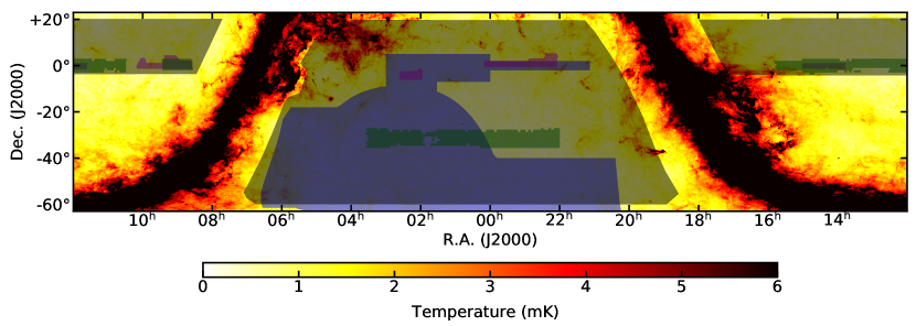
Figure 1: The ACT DR5 cluster search area (shaded in gray; covering 13,211 deg² after masking), overlaid on the Planck 353 GHz map, which is sensitive to thermal emission by dust. The footprints of deep and wide optical surveys that will provide weak-lensing mass calibration of the cluster sample are highlighted: DES (blue); HSC (magenta); and KiDS (green).

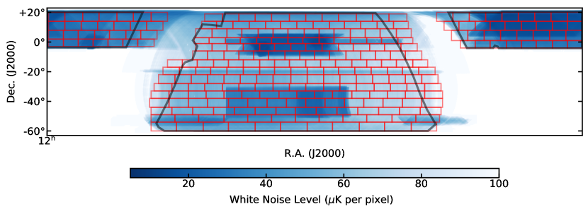
Figure 2: A map of the white noise level in the 150 GHz map, as produced by the map maker. The 98 and 150 GHz maps, which cover 18,000 deg² in total, are broken into tiles (marked in red) before filtering, for the reasons outlined in Section 2.2. The black outline marks the cluster search region, before the dust and point source masks are applied.

The ACT experiment saw first light in 2007, and since 2016 has been observing with its third generation receiver, Advanced ACTPol (AdvACT; Henderson et al., 2016). AdvACT consists of three detector arrays containing dichroic, dual polarization horn-coupled Transition Edge Sensor (TES) bolometers, observing at 98, 150, and 220 GHz, with 27 and 39 GHz channels added in the 2020 season. For this work, we use data from only the 98 and 150 GHz channels, which have approximate beam FWHM 2.2′ and 1.4′ respectively.

The cluster search was performed on co-added maps containing ACT data obtained between 2008–2018 (made available to the community as ACT DR5). The ACT maps for the 2008–2016 observing seasons are publicly available on the LAMBDA website, with seasons 2013–2016 being processed for ACT DR4 (Aiola et al., 2020; Choi et al., 2020). ACT DR5 contains co-added maps that incorporate early versions of the 2017–2018 data (N20), and unlike previous ACT data releases, includes observations taken during daylight hours. These maps have not been subjected to the full battery of tests needed for precision measurements of the CMB power spectrum, and may contain gain errors at the level of a few per cent. They are, however, much deeper over a much wider area than the maps used in the ACT DR4 analysis. More than 12,000 deg² (91% of the 13,211 deg² cluster search area) has noise level $<30$ $\mu$K-arcmin at 150 GHz (N20).

The co-added maps used in this work were produced in a two-step procedure (described in detail in N20). Individual maximum likelihood maps were first made for each observing season, frequency, and detector array, following the procedures described in Dünner et al. (2013) and Aiola et al. (2020). These maps were then combined into a single map per frequency, convolved to a common beam, by breaking each map into a series of tiles and weighting by a noise model constructed from the hitcount-modulated 2d noise power spectrum for each tile.

The co-added maps cover a sky area of approximately 18,000 deg². However, several thousand square degrees correspond to low Galactic latitudes ($|\,b\,|<20$ deg), where either the level of dust emission is high (making cluster detection in our mm-wave maps problematic), or the stellar density is high (making optical confirmation and redshift measurements difficult or impossible). Therefore, we defined the cluster search area (plotted over the Planck 353 GHz map in Fig. 1) to exclude such regions. We also mask dusty regions within the cluster search region, defined as pixels with temperature $>0.004$ K (in CMB temperature units) in the Planck 353 GHz map. We initially masked the locations of point sources detected in the ACT 150  GHz map using circular regions with radii in the range 3–12′, depending on the amplitude of the source at 150 GHz. After visual inspection of the filtered maps (see Section 3.2), we found it necessary to mask some regions that were not captured by the above procedures. Typically these were cases where our automated procedure to define source masking had not selected a large enough masking radius. We subsequently masked the locations of all sources with 150 GHz flux density $>10$ mJy (approximately 11,000 objects) using circles with radius 320″, except for those sources located within 9′ of bright clusters (with $\tilde{y}_{0}>1\times 10^{-4}$; $\tilde{y}_{0}$ is our chosen SZ observable, defined in Section 2.3 below), which are not masked (because “ringing” around bright clusters can be detected as spurious sources). After masking, the cluster search area is 13,211 deg².

2.2 Cluster Detection

We search for clusters using a multi-frequency matched filter (e.g., Melin et al., 2006; Williamson et al., 2011), applied to the 98 and 150 GHz maps,

$$\psi(k_{x},k_{y},\nu_{i})=A\sum_{j}\textbf{N}^{-1}_{ij}(k_{x},k_{y})f_{\rm SZ}(\nu_{j})S(k_{x},k_{y},\nu_{j})\,.$$ (1)

where $\psi$ is the filter, ($k_{x}$, $k_{y}$) denote the spatial frequencies in the horizontal and vertical directions in the maps, N is the noise covariance between the maps at different frequencies $\nu$, $S$ is a beam-convolved signal template, and $A$ is a normalization factor chosen such that, when applied to a set of maps containing a beam-convolved cluster signal (in temperature units), the matched filter returns the central Comptonization parameter (see Section 2.3 below). We use the non-relativistic form for the spectral dependence of the SZ effect given by

$$f_{\rm SZ}=x\frac{e^{x}+1}{e^{x}-1}-4\,,$$ (2)

where $x=h\nu/k_{B}T_{\rm CMB}$. We adopt 97.8 GHz and 149.6 GHz as the thermal SZ-weighted band centers for the 98 and 150  GHz maps analyzed here. These are the median values of the SZ-weighted band centers of the individual detector arrays; in practice the effective band centers vary slightly by position on the sky - see the Appendix of N20 - with uncertainty $\approx 1$ GHz on arcmin scales.

We use the map itself to form the noise covariance N, as the maps are dominated by the CMB on large scales, and white noise on small scales, rather than by the thermal SZ signal. Note that the filter is 2d in Fourier space, in order to account for the anisotropic noise that arises due to the scan pattern of ACT (e.g., Marriage et al., 2011), which varies according to position on the sky. However, the signal template $S$ is axisymmetric. We fill holes in the map created by point source masking (see Section 2.1) with a heavily smoothed version of the map itself prior to Fourier transforming.

As in previous ACT cluster searches (Hasselfield et al., 2013; Hilton et al., 2018), throughout this work we model the cluster signal using the Universal Pressure Profile (UPP; Arnaud et al., 2010, A10 hereafter), which is convolved with the appropriate ACT beam for each frequency to form the signal template $S$. To improve the detection efficiency for clusters with different angular sizes, we create a set of 16 matched filters, corresponding to $M_{\rm 500c}\in\{(1,2,4,8)\times 10^{14}$ $M_{\sun}\}$ and $z\in\{0.2,0.4,0.8,1.2\}$.

The ACT maps cover approximately 18,000 deg² and the noise level in the maps varies considerably as a function of position on the sky (see Fig. 2). In addition, the maps are produced in plate carrée projection (CAR in the terminology of FITS world coordinate systems; Calabretta & Greisen 2002), which leads to distortion away from the celestial equator as the solid angle covered by a pixel changes with declination. Therefore, we break the maps into a set of 280 tiles, each with approximate dimensions 10 deg $\times 5$ deg (right ascension $\times$ declination), and construct a different set of matched filters for each tile. Fig. 2 shows the layout of the tiles on the 150 GHz white noise level map (as produced by the map maker). Since we apodize each tile before Fourier transforming when constructing N, each tile is extended with a one degree wide border that overlaps with its neighbours.

To select cluster candidates, we construct a signal-to-noise ratio (SNR) map for each filtered tile, and in turn, make a segmentation map that identifies peaks with SNR $>4$. We estimate the noise map in a similar way to that used in Hilton et al. (2018), by dividing each tile into square 40$\arcmin$ cells and measuring the 3$\sigma$-clipped standard deviation in each cell, taking into account masked regions. This accounts for variations in depth within each tile. Finally, we apply the cluster search area mask shown in Fig. 1, and apply the dust and point source masks (see Section 2.1). Fig. 3 shows a comparison between the unfiltered 98 and 150 GHz maps, and a filtered map, after the application of all the above procedures.

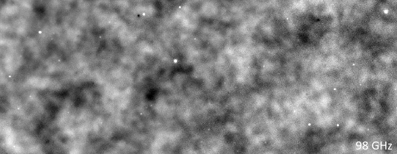
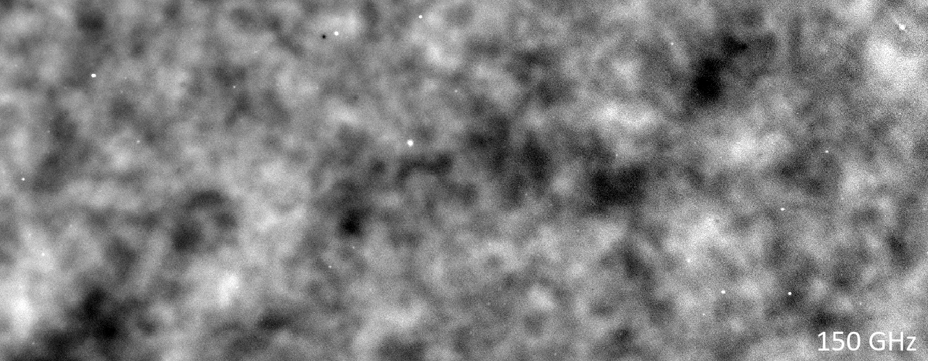
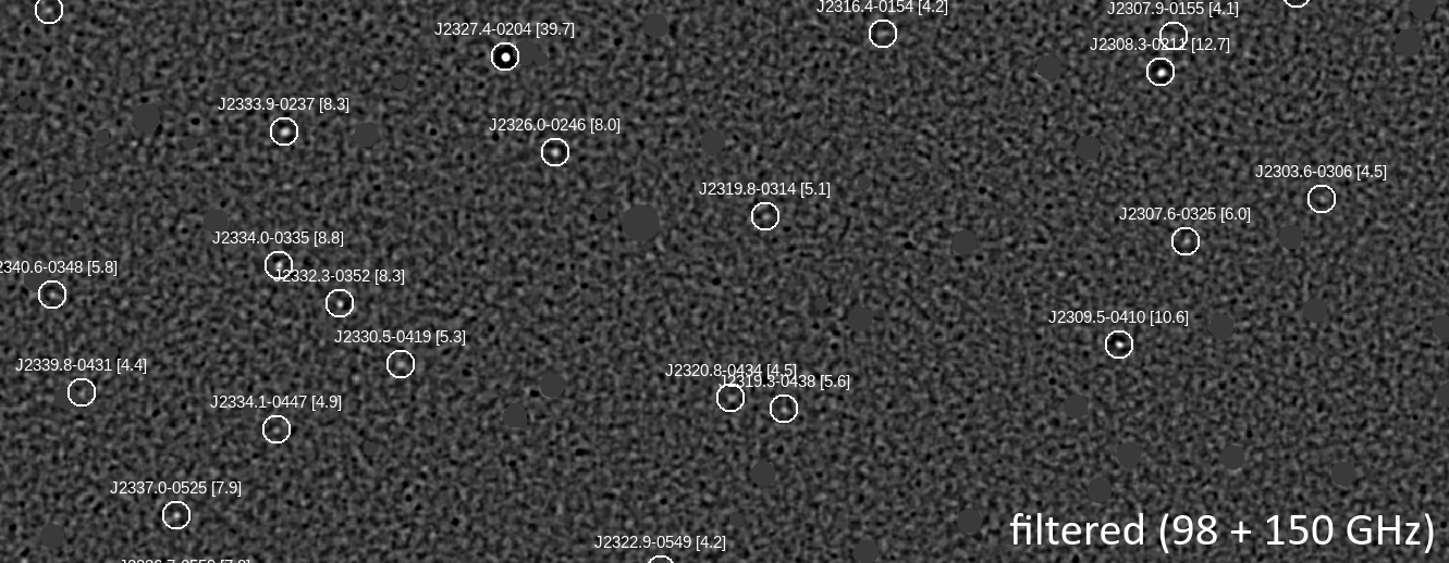
Figure 3: A comparison between the unfiltered 98 and 150 GHz maps, and the filtered signal-to-noise map, for an approximately $10$ deg$\times 4$ deg patch of sky. In the unfiltered maps, clusters appear as decrements (dark spots) in the map. Point sources appear as white spots, and CMB fluctuations dominate at large angular scales. In the filtered signal-to-noise map, clusters appear as white spots (marked with white circles to guide the eye; the number given in brackets is SNR_2.4), and point sources have been masked. The brightest object visible is the $z=0.70$ cluster ACT-CL J2327.4-0204 (center left, near the top left of the image), which is a SNR${}_{2.4}=39.7$ detection.

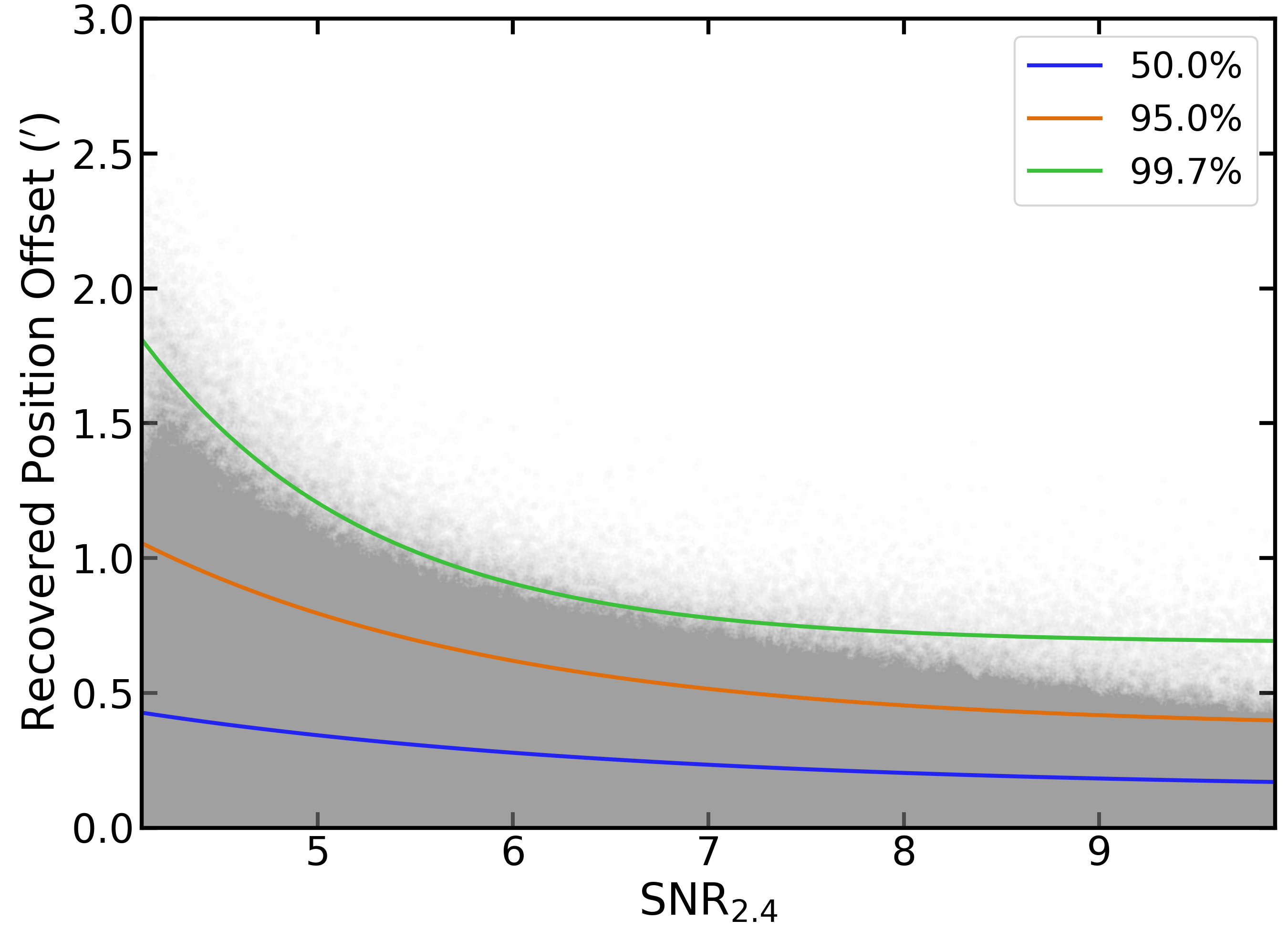
Figure 4: Accuracy of position recovery for injected UPP-model clusters, as a function of SNR_2.4. The offset with respect to the original input cluster position is plotted on the vertical axis. The gray points show the offsets recovered for individual model clusters. The solid lines show model fits of the form given in equation (3) that enclose the 50, 95, and 99.7 percentiles.

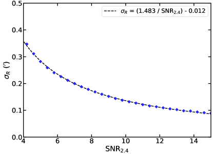
Figure 5: Results of fitting the distribution of recovered position offsets obtained from source insertion simulations using the Rayleigh distribution (equation 4). The simple model shown is a good description of how the scale parameter $\sigma_{R}$ changes as a function of SNR_2.4.

We assemble the final catalog of cluster candidates from a set of catalogs extracted from each SNR map for each filter scale in each tile, using a similar procedure to Hilton et al. (2018). We use a minimum detection threshold of a single pixel with SNR $>4$ in any filtered map, and adopt the location of the center-of-mass of the SNR $>4$ pixels in each detected object in the filtered map as the coordinates of each cluster candidate. We then create a final master candidate list by cross-matching the catalogs assembled at each cluster scale using a 1.4$\arcmin$ matching radius. Objects in the regions that overlap between tiles are removed by applying a mask; the tiles are defined such that each non-overlapping pixel in a tile maps to a unique pixel in the pixelization of the original monolithic map. We adopt the maximum SNR across all filter scales for each candidate as the ‘optimal’ SNR detection. However, as in Hasselfield et al. (2013) and Hilton et al. (2018), we also use a single reference filter scale (chosen to be $\theta_{\rm 500c}=2.4\arcmin$; see Section 2.3 below) at which we measure the cluster SZ signal and signal-to-noise ratio. Throughout this work we use SNR to refer to the ‘optimal’ signal-to-noise ratio (maximized over all filter scales), and SNR_2.4 for the signal-to-noise ratio measured at the fixed 2.4$\arcmin$ filter scale. The final catalog contains 8878 SNR $>4$ candidates selected from a survey area of 13,211 deg².

We checked the accuracy of recovered cluster positions by injecting simulated clusters into the maps and re-running the filtering and cluster detection procedures, taking care to remove objects corresponding to real cluster candidates from the resulting catalogs. The injected clusters are UPP models with uniformly distributed amplitudes and sizes selected from $\theta_{500c}(\arcmin{})\in\{7.8,4.2,2.4,1.5\}$. More than 5.7 million model clusters with $4<$ SNR${}_{2.4}<20$ are recovered from these simulations. We fit a model of the form

$$r=Ae^{-{\rm{SNR}_{2.4}}/B}+C\,,$$ (3)

where $r$ specifies the distance (in arcmin) between input and recovered model cluster positions within which some percentile of the objects are found, and $A$, $B$, and $C$ are fit parameters. Fig. 4 shows this model plotted over the position recovery data for the 50, 95, and 99.7 percentiles. The radial distance within which 99.7% of the model clusters are recovered is specified by a model with $A=38.1$, $B=1.16$, and $C=0.69$. We use this model for cross matching cluster candidates against external catalogs (see Section 3.2 below). Note that the accuracy of position recovery depends on cluster scale, with larger scale clusters having less accurately recovered positions, but for our purposes an average over several scales is sufficient.

For some applications (e.g., stacking on cluster positions), it is useful to model the positional uncertainty using the Rayleigh distribution, i.e.,

$$P(r,\sigma_{R})=\frac{r}{\sigma_{R}}\exp{\left(-r^{2}/2\sigma_{R}^{2}\right)}\,,$$ (4)

where $r$ is the distance between the true and recovered cluster position, and $\sigma_{R}$ is the scale parameter for the distribution. We fitted models of the form given in equation (4) to the distribution of recovered position offsets obtained from the source insertion simulations described above, binned by SNR_2.4. Fig. 5 shows the resulting measurements of $\sigma_{R}$ as a function of SNR_2.4, together with a simple model that captures how $\sigma_{R}$ changes with SNR_2.4.

We assess the number of false positive detections in the candidate list as a function of SNR_2.4 by running the cluster detection algorithm over sky simulations that are free of cluster signal. We use the map based simulations developed for Simons Observatory (Ade et al., 2019) for this purpose (Zonca et al., in prep.). We create maps at 93 and 145 GHz (the available bandpasses in the simulations are slightly different to ACT) on the N20 pixelization, containing a realization of the CMB plus the Cosmic Infrared Background (CIB) as implemented in WebSky (Stein et al., 2020). Since a complete model suitable for generating random realizations of the noise in the N20 maps is not currently available (and there are no splits of the N20 maps), we add white noise to the simulated maps following the levels in the N20 inverse variance maps. This means that the false positive rate inferred from these maps will be slightly optimistic, but as shown in Section 3.3, it is a reasonable match to the purity of the real cluster sample as assessed from regions with deep optical data. We apply all the same masks to the signal-free simulated maps as are used on the real maps, so the resulting catalog is drawn from a simulated survey with exactly the same area as the real ACT DR5.

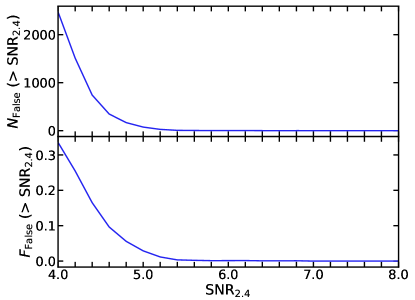
Figure 6: The number of false positive detections ($N_{\rm False}$; upper panel) above a given SNR_2.4 cut resulting from running the cluster finder on signal-free simulated maps with the same survey area, masks, and pixelization as the real N20 maps. The lower panel shows the fraction of false positives ($F_{\rm False}$) expected in the real ACT DR5 candidate list above a given SNR_2.4 cut. As shown in Section 3.3, the simple simulations used here are a reasonable match to the fraction of clusters recovered in regions where deep optical observations are used for confirmation.

The upper panel of Fig. 6 shows the number of detections in the signal-free simulation ($N_{\rm False}$) as a function of SNR_2.4 cut. For SNR${}_{2.4}>4$, we find there are 2471 false detections, falling to 75 for SNR${}_{2.4}>5$, and 2 for SNR${}_{2.4}>6$. For comparison, there are 7407 SNR${}_{2.4}>4$ candidates in the real candidate list (note that the full candidate list is not provided with this paper; we release only the catalog of optically confirmed clusters). Assuming that $N_{\rm False}$ is a reasonable estimate of the false positive rate in the real cluster candidate list, we can estimate the fraction of false positives as $F_{\rm False}=N_{\rm False}/N_{\rm Total}$, where $N_{\rm Total}$ is the number of objects in the real ACT DR5 candidate list. This is shown in the lower panel of Fig. 6. We find that $F_{\rm False}=0.34$ for SNR${}_{2.4}>4$, 0.03 for SNR${}_{2.4}>5$, and 0.001 for SNR${}_{2.4}>6$. Note that while these figures are a survey-wide average, we find little difference if we repeat this exercise considering only deeper parts of the map (e.g., $F_{\rm False}$ differs by $<2$% if we compare the footprint that overlaps with HSCSSP, where the ACT observations are deepest, with the whole survey footprint). We caution that these figures represent lower limits to the contamination rate in the candidate list, as the simulations used here do not capture all of the possible noise sources in the real maps. We compare $1-F_{\rm False}$ to the fraction of optically confirmed clusters in Section 3.3.

2.3 Cluster Characterization

In this work we continue to use the same approach to characterizing the SZ signal and its relation to mass as introduced in Hasselfield et al. (2013) and used in the ACTPol cluster search (Hilton et al., 2018). Briefly, we choose to characterize the SZ signal and survey completeness by selecting a single reference filter scale of angular size $\theta_{\rm 500c}=2.4$′, which corresponds to a UPP-model cluster with mass $M_{\rm 500c}=2\times 10^{14}$ $M_{\sun}$ at $z=0.4$ (close to the median redshift of the sample) for our fiducial cosmology. This avoids inter-filter noise bias, where local noise variations (e.g., the presence of CMB cold spots near candidates) can affect estimates of the cluster signal (and size) based on the maximal signal-to-noise filter scale (see the discussion in Hasselfield et al., 2013). However, we note that since the cluster finder still maximizes SNR over location on the sky, there is still a small positive bias in the recovered SNR values ($\approx 7$% at SNR${}_{2.4}=4.0$; see, e.g., Vanderlinde et al. 2010).

For a map filtered at the fixed 2.4′ reference scale, we assume that the cluster central Compton parameter $\tilde{y}_{0}$ is related to mass through

$$\tilde{y}_{0}=10^{A_{0}}E(z)^{2}\left(\frac{M_{\rm 500c}}{M_{\rm pivot}}\right)^{1+B_{0}}Q(\theta_{\rm 500c})f_{\rm rel}(M_{\rm 500c},z)\,,$$ (5)

where $10^{A_{0}}=4.95\times 10^{-5}$ is the normalization, $B_{0}=0.08$, $M_{\rm pivot}=3\times 10^{14}$ $M_{\sun}$, $Q(\theta_{\rm 500c})$ is the filter mismatch function ($\theta_{\rm 500c}=R_{\rm 500c}/D_{\rm A}$, where $D_{\rm A}$ is the angular diameter distance), and $f_{\rm rel}$ is a relativistic correction. $E(z)$ describes the evolution of the Hubble parameter with redshift, i.e., $E(z)=\sqrt{\Omega_{\rm m}(1+z)^{3}+\Omega_{\Lambda}}$. The parameter values for $10^{A_{0}}$, $B_{0}$ and $M_{\rm pivot}$ are equivalent to the A10 scaling relation, which was calibrated using X-ray observations. While this will typically result in masses that are lower than those calibrated against weak-lensing measurements (e.g., Miyatake et al., 2019, in the case of ACTPol), we choose to use the A10 relation here to ease comparison with our previous work. We also provide an alternative set of masses, rescaled via a richness-based weak-lensing calibration procedure, as described in Section 4.1.

The function $Q(\theta_{\rm 500c})$ in equation (5) accounts for the mismatch between the size of a cluster with a different mass and redshift to the reference model used to define the matched filter (including the effect of the beam) and in turn $\tilde{y}_{0}$ (see Section 3.1 of Hasselfield et al. 2013; Section 2.3 of Hilton et al. 2018). Since we break the map into tiles and construct a filter for each tile (Section 2.2), each tile has its own $Q(\theta_{\rm 500c})$ function.

We implement the relativistic correction $f_{\rm rel}$ applied in equation (5) differently in this work compared to previous ACT cluster surveys, which were based solely on 150 GHz data rather than the 98 and 150 GHz maps analyzed here. The size of $f_{\rm rel}$ depends on frequency, and is up to 1% larger at 150 GHz than 98 GHz for very massive clusters ($M_{\rm 500c}\approx 8\times 10^{14}$ $M_{\sun}$). We use the Arnaud et al. (2005) mass–temperature relation to convert $M_{\rm 500c}$ to temperature at a given cluster redshift, and then apply the formulae of Itoh et al. (1998) to calculate $f_{\rm rel}$ at each frequency. The filter $\psi$ defined in equation (1) returns the value $\tilde{y}_{0}$ when applied to a set of multi-frequency maps, weighting the contribution of each map to the returned SZ signal according to both the spectral dependence of the SZ signal (equation 2) and the noise in the map. We use these weights, which differ from tile to tile, to estimate an average $f_{\rm rel}$ for each cluster. The overall impact of the relativistic correction is small (approximately 3% for the median mass of the ACT DR5 cluster sample).

Equation (5) cannot be inverted to obtain the mass $M_{\rm 500c}$, due to the steepness of the cluster mass function and the presence of intrinsic log normal scatter $\sigma_{\rm int}$ in $\tilde{y}_{0}$ about the mean relation defined by equation (5). We adopt $\sigma_{\rm int}=0.2$ throughout this work, based on the results of numerical simulations (see Hasselfield et al., 2013). Given a cluster redshift measurement, mass estimates are extracted by computing the posterior probability

$$P(M_{\rm 500c}|\tilde{y}_{0},z)\propto P(\tilde{y}_{0}|M_{\rm 500c},z)P(M_{\rm 500c}|z)\,,$$ (6)

where $P(M_{\rm 500c}|z)$ is the halo mass function at redshift $z$, for which we use the fitting formulae of Tinker et al. (2008), as implemented in the Core Cosmology Library v2.1 (CCL; Chisari et al., 2019). We assume $\sigma_{8}=0.80$ for such calculations throughout this work. We account for the uncertainties on both $z$ and $\tilde{y}_{0}$ in calculating $P(M_{\rm 500c}|\tilde{y}_{0},z)$, and adopt the maximum of the $P(M_{\rm 500c}|\tilde{y}_{0},z)$ distribution as the cluster $M_{\rm 500c}$ estimate. The uncertainties quoted on these masses are $1\sigma$ error bars that do not take into account any uncertainty on the scaling relation parameters.

The mass estimates obtained through equations (5) and (6) are referred to as $M^{\rm UPP}_{\rm 500c}$ throughout this work. For comparison with some other works (e.g., the Planck PSZ2 catalog; Planck Collaboration et al. 2016b), it is sometimes necessary to neglect the Eddington bias correction (done by equation 6) that accounts for the steepness of the cluster mass function and intrinsic scatter (see the discussion in Battaglia et al. 2016 and Hilton et al. 2018). We label these ‘uncorrected’ masses as $M^{\rm Unc}_{\rm 500c}$.

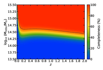
Figure 7: The completeness for SNR${}_{2.4}>5$ as a function of redshift, in terms of $M^{\rm UPP}_{\rm 500c}$, over the full 13,211 deg² survey footprint. The Tinker et al. (2008) halo mass function and Arnaud et al. (2010) scaling relation are assumed (see Section 2.4). The dashed black contour marks the 90% completeness limit.

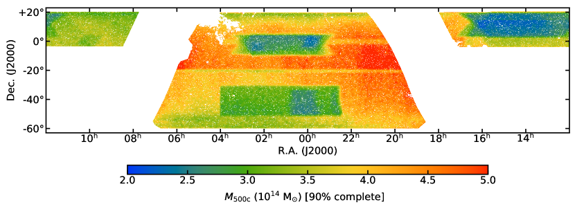
Figure 8: Map of the 90% completeness mass limit for SNR${}_{2.4}>5$ as a function of redshift, in terms of $M^{\rm UPP}_{\rm 500c}$, evaluated at $z=0.5$ (the median redshift of the detected clusters). The variation is driven by the ACT observing strategy.

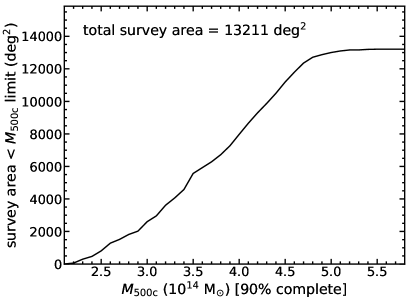
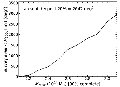
Figure 9: Mass sensitivity in terms of $M^{\rm UPP}_{\rm 500c}$, evaluated at $z=0.5$, as a cumulative function of area, for the whole survey (left), and for the deepest 20% (right).

2.4 Survey Completeness

We estimate the completeness of the survey in terms of mass using mock catalogs generated through Monte Carlo simulations. For speed, the calculations are performed on a redshift grid, covering the range $0<z<2$ in steps of size $\Delta z=0.01$. At each redshift step, we make 2 million draws from the Tinker et al. (2008) halo mass function, above a minimum halo mass of $M_{\rm 500c}>8\times 10^{13}$ $M_{\sun}$ (i.e., well below the expected mass limit). We then calculate the true value of $\tilde{y}_{0}$ for each of the randomly drawn halo masses using equation (5), assuming the scaling relation parameters derived from A10. Here we apply the appropriate filter mismatch function ($Q$) for the tile each mock cluster is located in, and apply the relativistic correction as described in Section 2.3. We then add Gaussian-distributed random noise to $\tilde{y}_{0}$, according to the level estimated in the $\tilde{y}_{0}$ noise map, and finally we add log-normal scatter to $\tilde{y}_{0}$ with size $\sigma_{\rm int}=0.2$ (see Section 2.3). After repeating this for each redshift step and each map tile (see Section 2.2), we have assembled an oversampled mock catalog containing true masses, redshifts, and mock $\tilde{y}_{0}$ values (and their uncertainties) over the full ACT DR5 cluster search area that extends well below the mass selection limit. We then project this catalog onto a ($\log_{10}M_{\rm 500c},z$) grid, and estimate the completeness as the fraction of the mock clusters in each ($\log_{10}M_{\rm 500c},z$) bin that are above a chosen SNR_2.4 detection threshold. We repeat this process 1000 times, taking the average as the estimate of the overall survey completeness.

Fig. 7 shows the 90% completeness limit as a function of redshift in terms of $M^{\rm UPP}_{\rm 500c}$ for SNR${}_{2.4}>5$ over the full 13,211 deg² survey area. Evaluated at $z=0.5$ (approximately the median redshift of the cluster sample; see Section 3), we estimate that the cluster catalog is 90% complete for $M^{\rm UPP}_{\rm 500c}>3.8{}\times 10^{14}\,M_{\sun}$. The survey is slightly more sensitive to lower mass clusters than this in areas that overlap with the DES, HSC, and KiDS optical surveys ($M^{\rm UPP}_{\rm 500c}>3.6\times 10^{14}\,M_{\sun}$). This statement relates only to the noise levels in the ACT maps in the regions of overlap, i.e., no optical information is used in deriving estimates of the survey mass limit.

There is a fairly large spatial variation in the mass completeness limit across the map, as shown in Fig. 8, which is driven by the ACT observing strategy. Fig. 9 shows the cumulative survey area as a function of the estimated mass completeness limit. Almost all of the vastly-increased survey area reaches a lower mass limit than previous ACT cluster surveys (Marriage et al., 2011; Hasselfield et al., 2013; Hilton et al., 2018). Clusters with masses in the range $2.1<M^{\rm UPP}_{\rm 500c}/10^{14}\,M_{\sun}<3.1$ can be detected in the deepest 20% of the survey, corresponding to an area of 2634 deg² – more than double the area searched in Hilton et al. (2018), and larger than the area searched in the SPT-SZ survey (Bleem et al., 2015b; Bocquet et al., 2019).

3 Optical/IR Follow-up and Redshifts

In this Section we describe the process of optical/IR confirmation of SZ-detected candidates as clusters of galaxies. The redshifts assigned to objects in the cluster catalog come from a variety of sources, because the ACT DR5 cluster search area is not covered by a single, deep optical/IR survey. We have attempted to obtain as many reliable redshift estimates as possible, given the data available. We provide details on each of the redshift sources in Section 3.1 below. Section 3.2 summarizes the process of cross matching the cluster candidate list against external catalogs, visual inspection of the available optical/IR data, and the process by which we adopted a single redshift measurement for each cluster. We comment on redshift follow-up completeness and the purity of the cluster candidate list in Section 3.3.

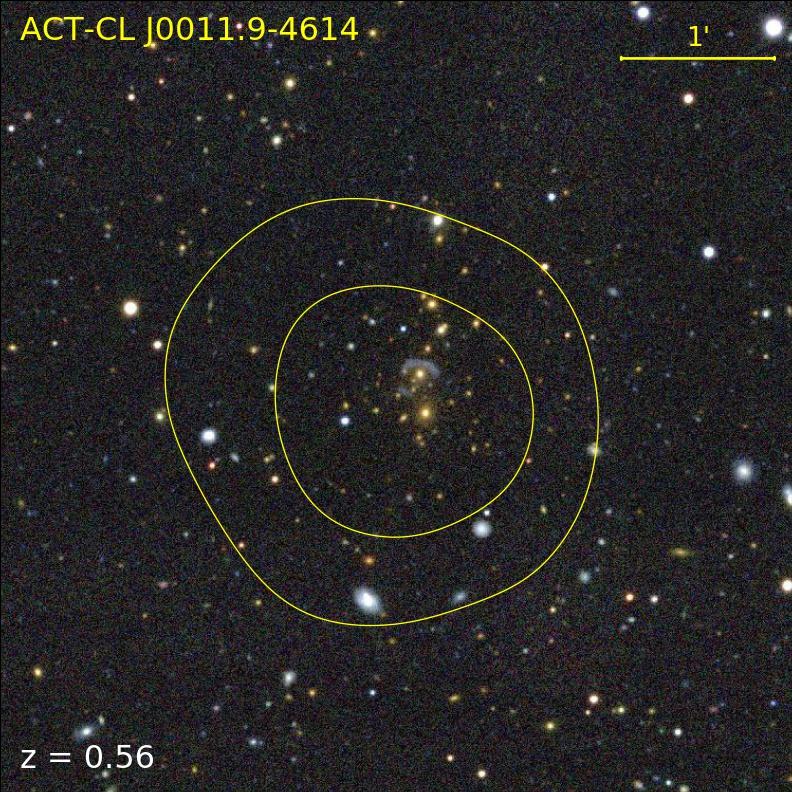
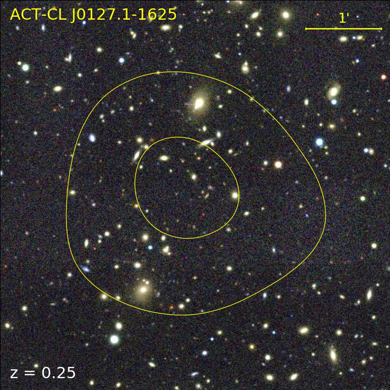
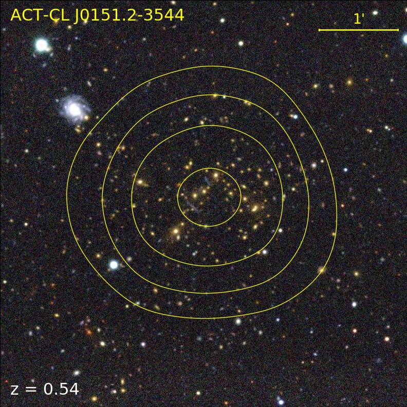
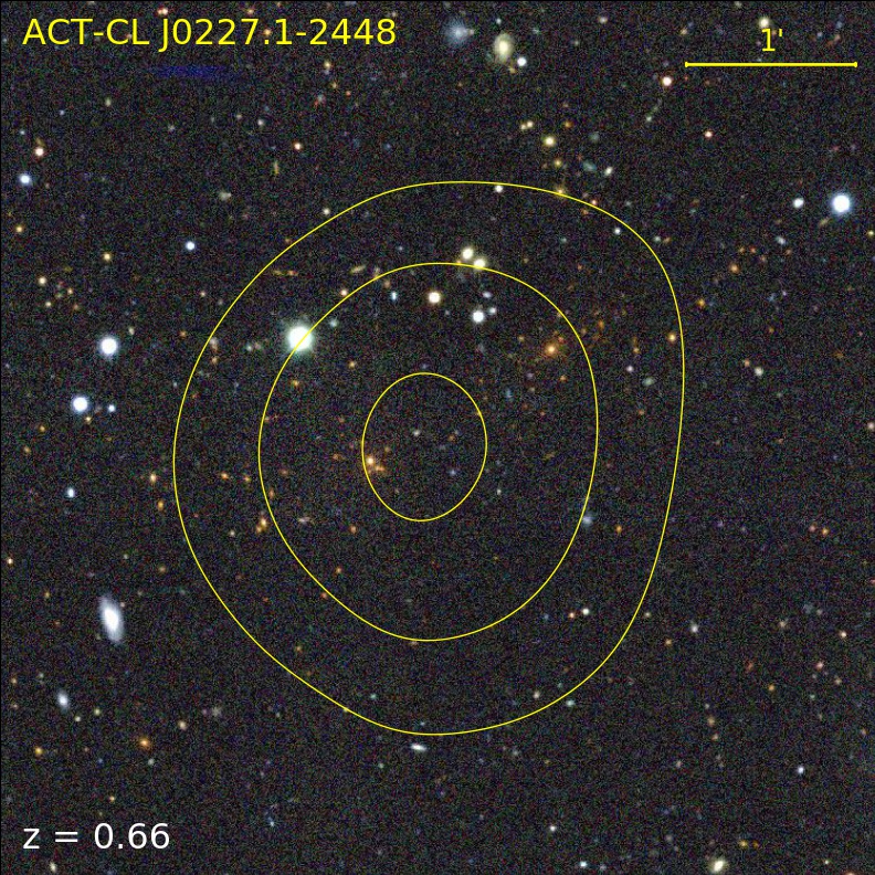
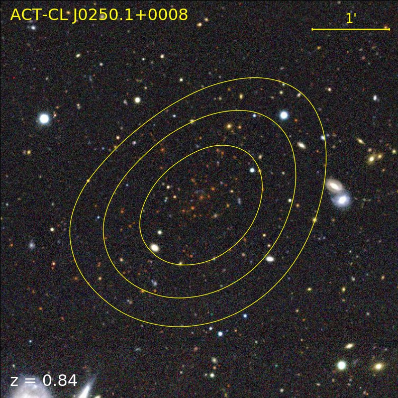
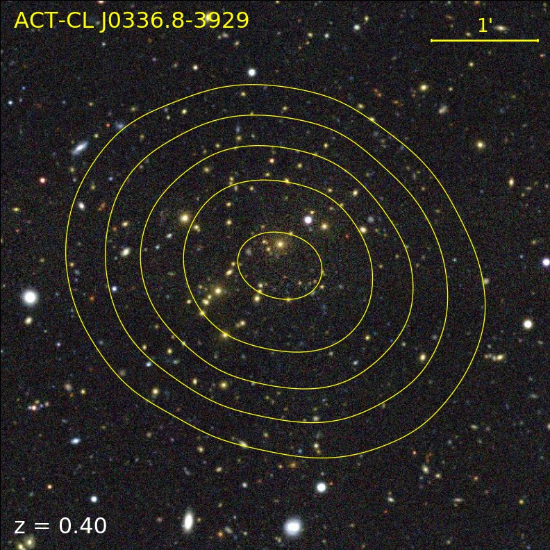
Figure 10: Example DES $gri$ images of ACT DR5 clusters at various redshifts confirmed using redMaPPer. Each image is 5′ on a side, with North at the top, East at the left. The contours mark signal-to-noise ratio in the ACT map filtered at the reference 2.4′ scale. The lowest level shown corresponds to 3$\sigma$ significance, and each subsequent level is 2$\sigma$ higher.

3.1 Redshift Sources

3.1.1 Large Public Spectroscopic Surveys

The large ACT DR5 survey area overlaps with several large public spectroscopic surveys. In this work we made use of 2dFLenS (Blake et al., 2016), OzDES (Childress et al., 2017), SDSS DR16 (Ahumada et al., 2020), and VIPERS (Scodeggio et al., 2018). We cross matched the cluster candidate list against each of these surveys in turn, and estimated cluster redshifts using an iterative procedure similar to that used in Hilton et al. (2018). For each cluster in the list, we first select only galaxies with secure spectroscopic redshifts located within a projected distance of 1 Mpc from the cluster SZ position. We then iteratively estimate the cluster redshift using the biweight location estimator (e.g., Beers et al., 1990), keeping only galaxies with peculiar velocities within 3000 km s^-1 of the cluster redshift estimated at each iteration. In some iterations, there may be no galaxies found within these peculiar velocity limits (e.g., on rare occassions where the redshift distribution is bimodal). In these cases, we disregard the peculiar velocity cut, and take the median of all the galaxy redshifts as the cluster redshift estimate, before beginning the next iteration. This procedure typically converges within a couple of iterations.

SDSS DR16 provides the vast majority of spectroscopic redshifts assigned to clusters in the final catalog (1123), followed by 2dFLens (56), OzDES (3), and VIPERS (2). Note that following visual inspection of optical imaging (Section 3.2), we rejected 56 cases of erroneous redshift estimates produced by the above automated procedure in favour of a “manually assigned” spectroscopic redshift (e.g., based on an obvious brightest central galaxy). These objects are flagged in the warnings field of the cluster catalog (see Table 1).

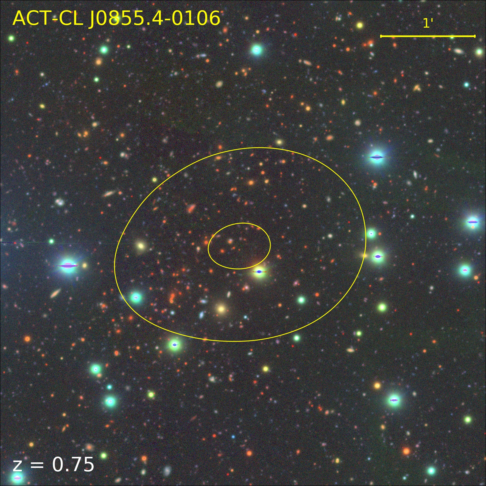
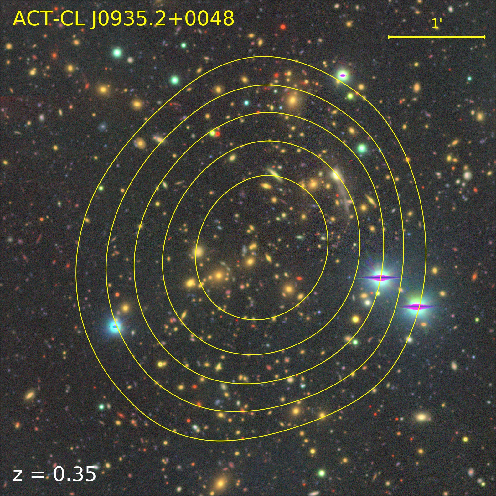
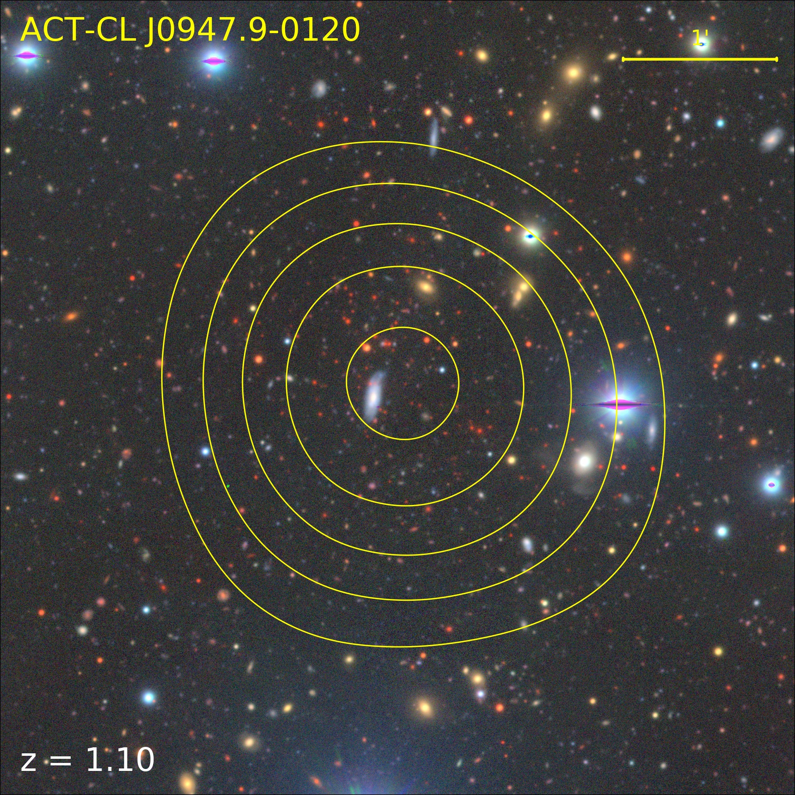
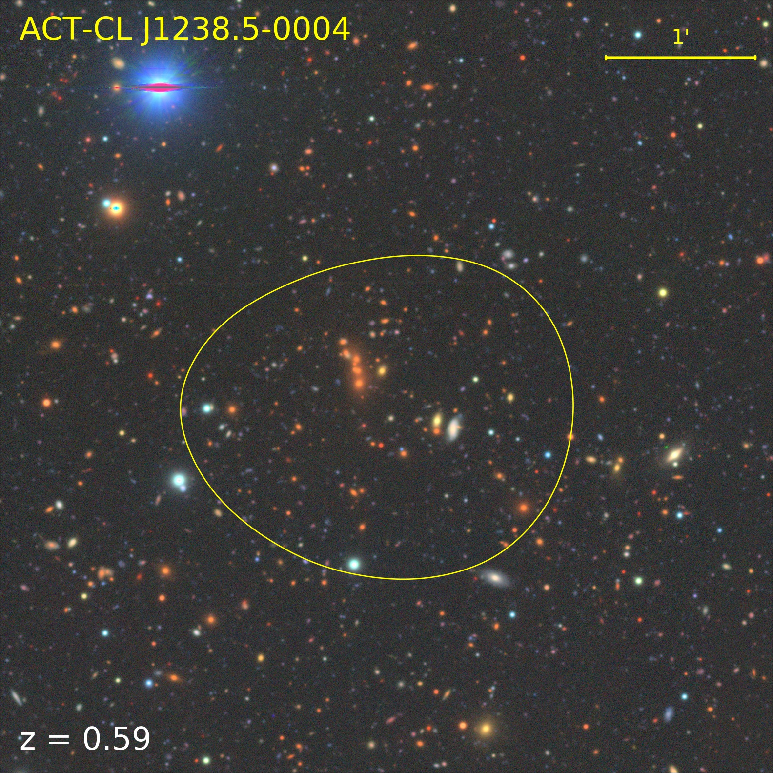
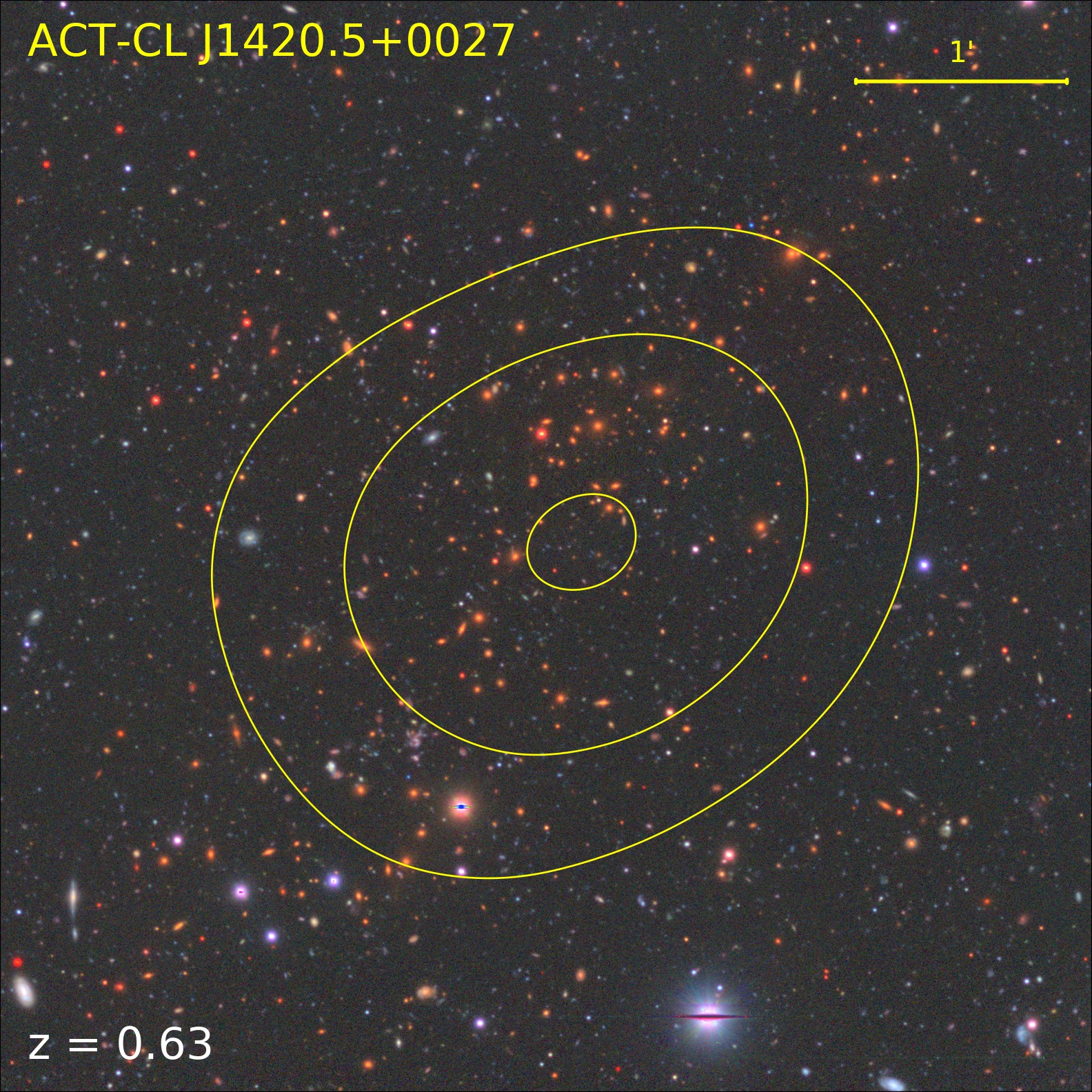
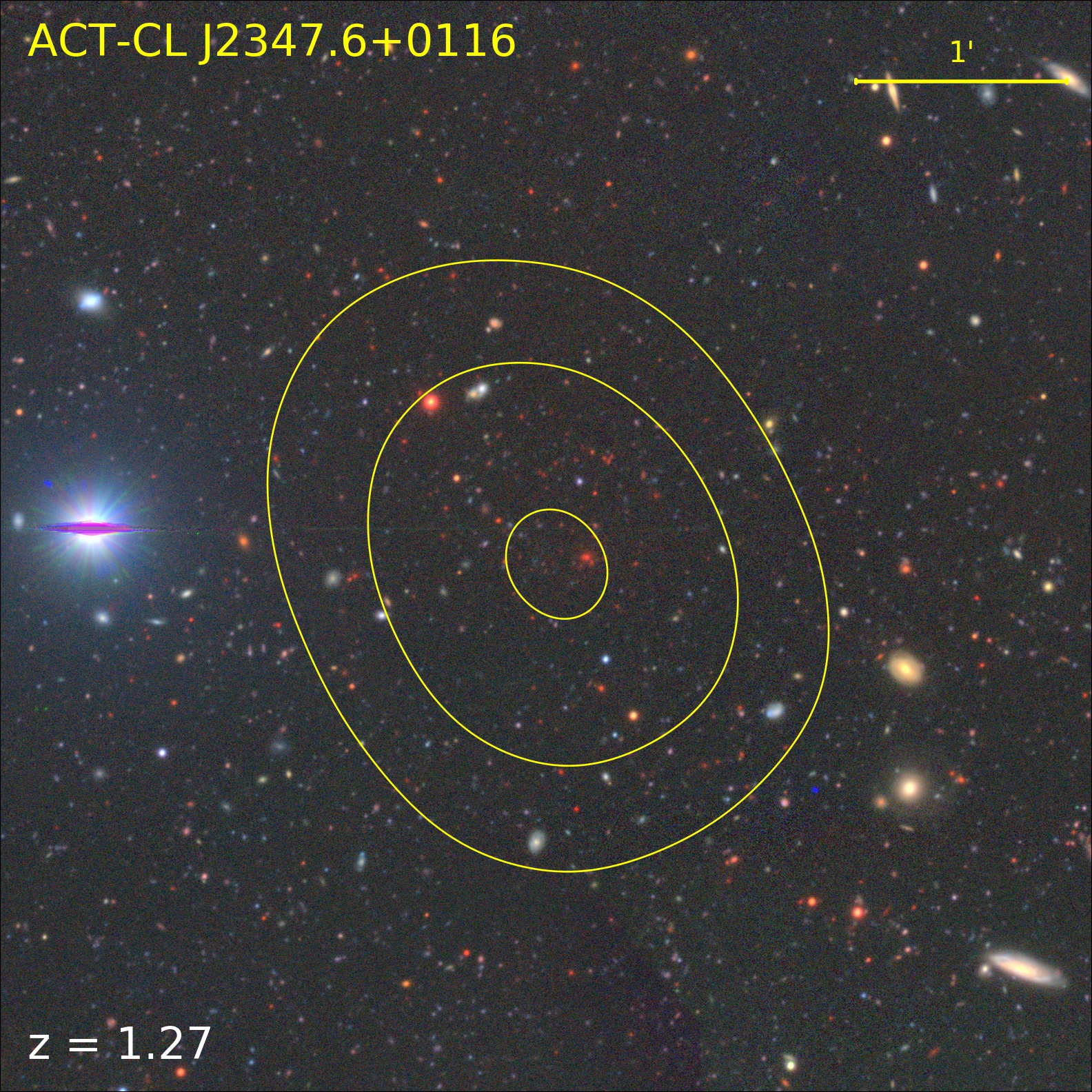
Figure 11: Example $gri$ images of ACT DR5 clusters at various redshifts, confirmed using HSC imaging and the CAMIRA optical cluster finder. Each image is 5′ on a side, with North at the top, East at the left. The ACT signal-to-noise contours have the same scaling as in Fig. 10.

3.1.2 Photometric Redshifts From RedMaPPer

The cluster search area has a large overlap with SDSS (in equatorial regions) and 4566 deg² in common with the deep $griz$ imaging provided by DES - i.e., almost all of the DES footprint (see Fig.1). The DES data used in this work come from the first three years of observations (referred to throughout this paper as “DES Y3”), for which the imaging and photometric catalogs are publicly available as DES DR1 (Abbott et al., 2018).

RedMaPPer is an optical red-sequence based cluster finding algorithm that was applied to $ugriz$ SDSS data (Rykoff et al., 2014), and has subsequently been developed to run on DES photometry (Rykoff et al., 2016). In SDSS, redMaPPer is able to find clusters out to $z\approx 0.5$, while the increased depth of DES allows it to find clusters out to $z\approx 0.9$. One of the key features of redMaPPer is its optical richness measurement ($\lambda$), which has been shown to scale with cluster mass (e.g., Simet et al., 2017; McClintock et al., 2019). The photometric redshift estimates provided by redMaPPer are very accurate, with $\sigma_{z}/(1+z)<0.02$ over the full redshift range probed in each survey.

In this work we use the public SDSS redMaPPer catalog (v6.3; Rykoff et al., 2014) and a new redMaPPer catalog based on the DES Y3 photometry (v6.4.22), containing 33,654 clusters. Both catalogs contain only $\lambda>20$ systems; at this richness, only $5-7$% of the clusters are expected to be projections along the line of sight (Rykoff et al., 2014, 2016). Since the SZ-selected ACT DR5 cluster catalog may contain clusters at high redshift ($z>0.8$) that may not be found by redMaPPer alone, we also ran redMaPPer in ‘scanning mode’, using the prior information of the ACT cluster candidate positions. We found that there is 5% chance association probability of detecting a $\lambda>20$ system by using redMaPPer in this mode, from a test based on a mock ACT DR5 catalog containing $>93,000$ random positions within the DES Y3 footprint, generated from the $\tilde{y}_{0}$ noise map. Note that this represents the average chance association probability; it is possible that this quantity varies with redshift (see the treatment in Klein et al., 2019). Bleem et al. (2020) applied the redMaPPer scanning mode to the SPT Extended Cluster Survey (SPT-ECS), and report a similar chance association probability to that which we find between ACT DR5 and redMaPPer.

We adopted redMaPPer redshifts for 1433 clusters in the ACT DR5 catalog (256 from SDSS, 1023 from DES Y3, and a further 154 from the ‘scanning mode’ run in DES Y3). This is the most from any of the redshift sources used in this work. Fig. 10 shows some example images of clusters confirmed using redMaPPer in DES Y3.

3.1.3 Photometric Redshifts from CAMIRA

The Hyper Suprime-Cam Subaru Strategic Program (HSC-SSP) is a deep optical $grizy$ survey reaching to depths fainter than 26th magnitude in the $r$-band (Miyazaki et al., 2018; Aihara et al., 2018). The HSC-SSP full-depth full-color (FDFC) footprint corresponding to observations up to the 2019A semester has 469 deg² of overlap with the ACT DR5 cluster search area, as shown in Fig. 1.

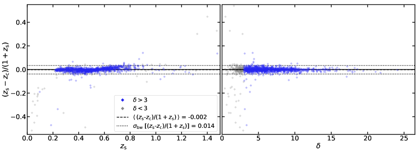
Figure 12: The left panel shows a comparison of spectroscopic redshifts ($z_{s}$) with zCluster photometric redshifts ($z_{c}$) based on DECaLS DR8 photometry. More than 98% of the objects are recovered within $\Delta z/(1+z_{\rm s})<0.05$ of the spectroscopic redshift. Note that a bias correction of the form $z=z_{\rm c}+0.02(1+z_{\rm c})$ has been applied to the photometric redshifts. The right panel illustrates how the scatter in the photometric redshifts varies with the $\delta$ statistic. Objects with $\delta>3$ are highlighted; many objects with $\delta$ below this threshold have accurate redshift estimates, but the scatter is much larger.

An optical cluster finding algorithm named CAMIRA (Cluster finding Algorithm based on Multi-band Identification of Red-sequence gAlaxies; Oguri, 2014), which is similar to redMaPPer but was developed independently, has been run on the HSC data. Here we use the CAMIRA cluster catalog based on HSC-SSP S19A photometry; note that the CAMIRA cluster search uses a less conservative mask and covers slightly more area than the FDFC mask. The photometric redshift estimates provided by CAMIRA have low scatter ($\sigma_{z}/(1+z)=0.008$ at $z<1.1$; $\sigma_{z}/(1+z)\approx 0.02$ for $z>1.1$), and reach to $z\approx 1.4$ (higher than the $z<1.1$ limit in the S16A catalog; Oguri et al., 2018). The richness measure used in CAMIRA ($N_{\rm mem}$) counts the number of red-sequence galaxies in a background-corrected circular aperture, in a similar manner to the $\lambda$ quantity used in redMaPPer (see Oguri 2014 for a detailed definition). Similarly to redMaPPer, we also ran CAMIRA in ‘scanning mode’, using prior information of ACT candidate positions. We find that the 5% chance association probability corresponds to a richness threshold of $N_{\rm mem}>16$, by running the algorithm on a catalog of random positions drawn from a mock ACT DR5 cluster catalog. We use this to set the minimum $N_{\rm mem}$ threshold when considering cross matches against the CAMIRA catalog.

We adopted redshifts for 58 clusters from CAMIRA (only 7 of these are from the ‘scanning mode’ run). Fig. 11 shows some example clusters confirmed using CAMIRA.

3.1.4 Photometric Redshifts From zCluster

The zCluster algorithm, described in Hilton et al. (2018), estimates redshifts for galaxy clusters using broadband photometry, given a priori knowledge of the cluster position. This is done using a weighted sum of the redshift probability distributions for galaxies along the line of sight to a cluster candidate. In addition to the redshift estimate, zCluster also provides a measure of optical density contrast,

$$\delta(z_{\rm c})=\frac{n_{\rm 0.5\,Mpc}(z_{\rm c})}{An_{\rm 3-4\,Mpc}(z_{\rm c})}-1\,,$$ (7)

where $z_{\rm c}$ is the estimated photometric redshift for the cluster, $n_{\rm 0.5\,Mpc}(z_{\rm c})$ is the number of galaxies within 0.5 Mpc projected distance of the given cluster position, $n_{\rm 3-4\,Mpc}(z_{\rm c})$ is a measure of the background number of galaxies in a circular annulus 3–4 Mpc from the cluster position, and $A$ is a factor that accounts for the difference in area between these two count measurements. As shown in Hilton et al. (2018), a $\delta$ threshold can be used to identify cluster candidates with unreliable redshift estimates.

In this work, we applied zCluster to photometric data from the Dark Energy Camera Legacy Survey (DECaLS DR8; Dey et al., 2019), the Kilo Degree Survey (KiDS DR4; Wright et al., 2019), and SDSS (DR16; Ahumada et al., 2020). DECaLS provides optical $grz$ photometry combined with 3.4, 4.6 µm photometry from the Wide-field Infrared Survey Explorer mission (WISE; Wright et al., 2010), and covers most of the ACT DR5 cluster search area footprint (10,822 deg² of overlap). We find that zCluster is able to measure cluster redshifts out to $z\approx 1.4$ when applied to DECaLS, due to the inclusion of the WISE data. KiDS DR4 provides ugriZYJHK_s photometry over 825 deg² in common with ACT DR5, with near-infrared data provided by the VISTA Kilo degree Infrared Galaxy survey (VIKING; Edge et al., 2013).

This work benefits from several improvements that have been made to zCluster, which we briefly summarize here: (i) a new automated masking procedure, that constructs an area mask image using the positions of objects in the catalog and the typical nearest-neighbour separation, resulting in more accurate $\delta$ estimates close to survey boundaries; (ii) bootstrap resampling is used to estimate the uncertainty on the density contrast statistic ($\Delta\delta$) at all points along the redshift range, and redshifts at which $\delta/\Delta\delta<3$ are rejected; and (iii) we have added the ability to easily swap the spectral template set used for the individual galaxy photometric redshift estimates.

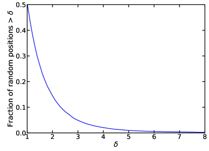
Figure 13: Fraction of random positions drawn from a mock ACT DR5 cluster catalog where $\delta$, the zCluster density contrast statistic as measured using DECaLS photometry, is greater than some value. We find $\delta>3$ for 5% of the random points.

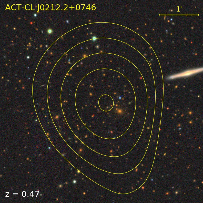
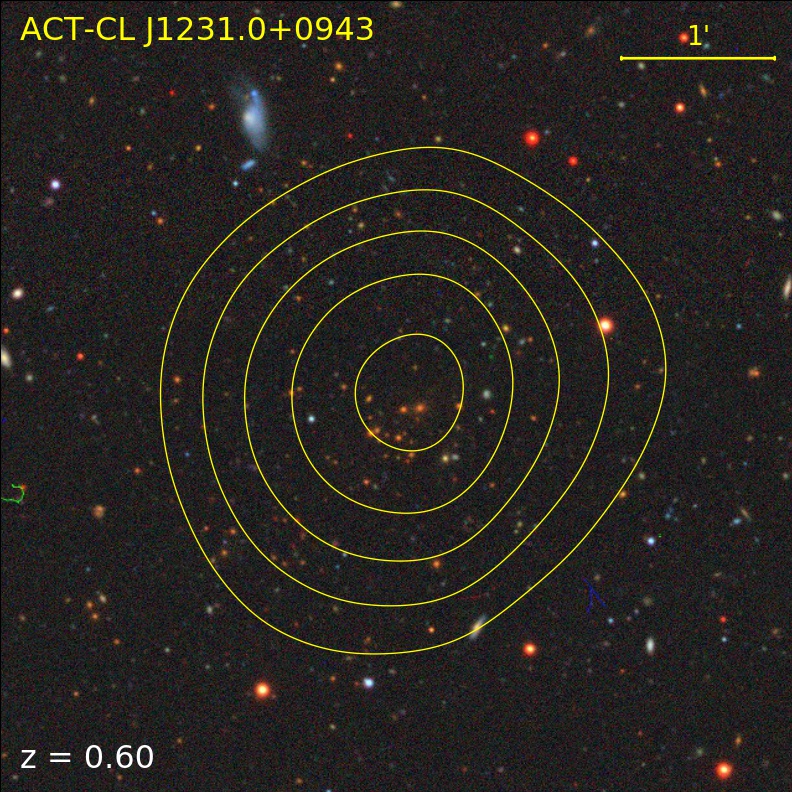
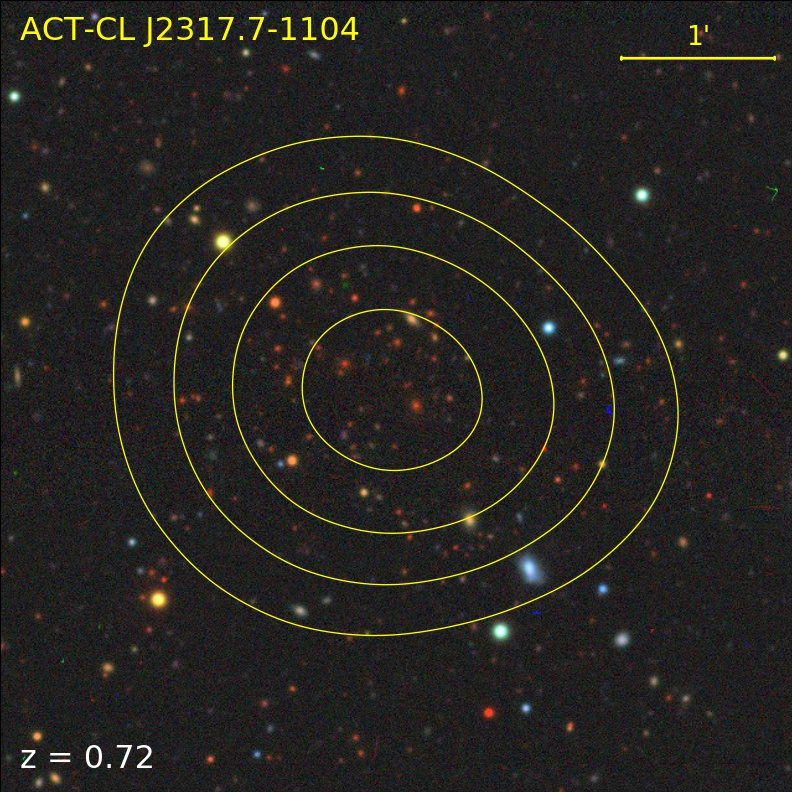
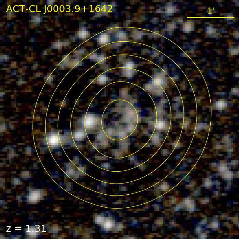
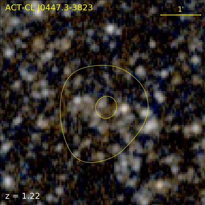
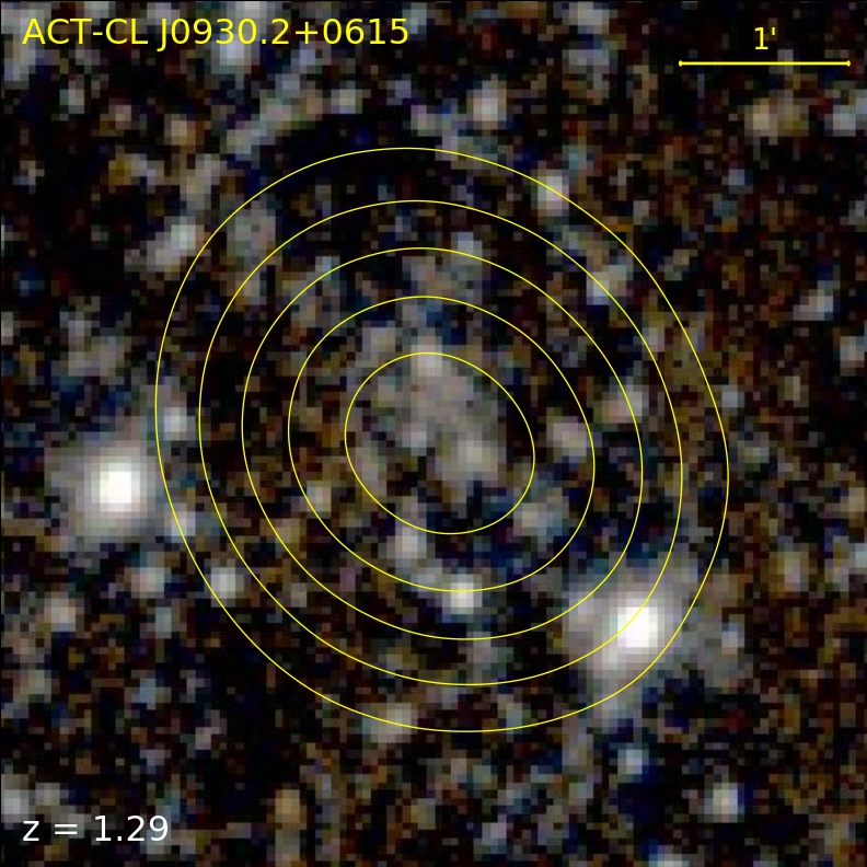
Figure 14: Example DECaLS $grz$ images of ACT DR5 clusters at $z<0.8$ (top row) and unWISE images of $z>1$ ACT DR5 clusters (bottom row). Each image is 5′ on a side, with North at the top, East at the left. See Fig. 10 for an explanation of the contour levels.

While we ran zCluster on SDSS and KiDS photometry using the same set of spectral templates as used in Hilton et al. (2018), i.e., the default templates from the EAZY photometric redshift code (Brammer et al., 2008), supplemented by the Coleman et al. (1980, CWW hereafter) templates, we found it necessary to switch the spectral template set in order to optimize the performance when running on DECaLS photometry. We used a subset of the spectral templates used in the COSMOS survey (Ilbert et al., 2009; Salvato et al., 2011), representing a range of normal galaxies and AGNs, removing all elliptical templates based on Bruzual & Charlot (2003) stellar population synthesis models (as these were found to give biased results for individual galaxies at moderate redshifts; we speculate that this is probably related to the extrapolation of the stellar population synthesis models into the WISE bands), and adding in the CWW template set.

Fig. 12 presents a comparison between 1168 clusters with spectroscopic redshifts ($z_{\rm s}$) and zCluster photometric redshift estimates ($z_{\rm c}$), based on DECaLS photometry. Note that we have corrected the zCluster redshifts for a bias of the form $z=z_{\rm c}+0.02(1+z_{\rm c})$, where $z$ represents the corrected photometric redshift. We have not identified the source of this bias as yet, but note that this correction is sufficient to ensure that on average the zCluster redshifts reported in this work are not biased. As shown in Fig. 12, for clusters with $\delta>3$, the scatter in the redshift residuals $\Delta z/(1+z_{\rm s})$ is small ($\sigma_{\rm bw}=0.014$; estimated using the biweight scale, e.g., Beers et al. 1990). The scatter rises to $\sigma_{\rm bw}=0.04$ for the 16 objects beyond $z>1$. We find that 98% of the redshifts are recovered within $\Delta z/(1+z_{\rm s})<0.05$ of the spectroscopic redshift, so the number of catastrophic outliers is small.

To estimate the probability of a cluster candidate being associated with a random position on the sky where $\delta>3$, we ran zCluster on DECaLS photometry on the same mock cluster catalog used for similar tests of redMaPPer and CAMIRA (Sections 3.1.2 and 3.1.3 above). Fig. 13 shows the results of this exercise. We find that 5% of random positions have $\delta>3$, rising to 14% for $\delta>2$ and 26% for $\delta>1.5$. Nevertheless, as shown in the right panel of Fig. 12, the zCluster photometric redshift estimates largely remain accurate at $\delta<3$: we find $\sigma_{\rm bw}=0.018$ for objects with $2<\delta<3$, with 95% of these objects being found within $\Delta z/(1+z_{\rm s})<0.05$ of the spectroscopic redshift.

Fig. 14 presents images of some example clusters confirmed using zCluster and DECaLS. The ACT DR5 cluster catalog contains 717 objects with redshifts provided by zCluster (706 based on DECaLS photometry, 4 based on KiDS data, and 7 based on SDSS DR16). For 13 of the measurements based on DECaLS, we applied a $z>0.6$ prior to avoid confusion with projected lower $z$ systems that were judged not to be the source of the SZ signal following visual inspection of the available imaging. In 96 cases where no alternative estimate is available, we adopt zCluster redshifts with $\delta<3$. All of these exceptions are appropriately flagged in the warnings field of the cluster catalog (see Table 1).

3.1.5 Spectroscopic Redshifts From BEAMS

The BEAMS project (Brightest cluster galaxy Evolution with ACT, MeerKAT, and SALT) is a Large Science Program on the Southern African Large Telescope (SALT) that is obtaining long-slit spectroscopic observations of around 150 cluster central galaxies in a representative sample of $0.3<z<0.8$ ACT clusters. BEAMS observations began in May 2019 and at the time of writing 54 clusters have been observed. The SALT data in hand have been processed with a modified version of the pipeline described in Hilton et al. (2018). In this work, we report spectroscopic redshifts from BEAMS (labeled SALTSpec in Table 2) for 15 clusters that would otherwise have only photometric estimates.

3.1.6 Other Redshift Sources

We adopted a large number of redshifts used in the ACT DR5 cluster catalog from various sources in the literature. In particular, we used redshifts from previous published SZ surveys by ACT (Menanteau et al., 2013a; Sifón et al., 2016; Hilton et al., 2018), Planck (Planck Collaboration et al., 2016b), and SPT (Bleem et al., 2015b, 2020; Bocquet et al., 2019); optically selected cluster catalogs based on SDSS (Wen et al., 2012; Wen & Han, 2015, labelled as ‘WHL’ in this work), KiDS DR3 (Maturi et al., 2019, photometric redshifts based on the AMICO cluster finding algorithm), and ESO ATLAS (Ansarinejad et al., 2020, photometric redshifts based on the ORCA cluster finding algorithm; Murphy et al. 2012); and the IR-selected Massive Distant Clusters of WISE survey (MaDCoWS; Gonzalez et al., 2019), which contains more than 2000 high redshift ($0.7<z<1.5$) clusters selected from a survey area that covers most of the extragalactic sky.

We collected a large number of redshifts using the NASA Extragalactic Database (NED). We took care to classify such redshifts as spectroscopic or photometric with appropriate uncertainties. References for these miscellaneous sources can be found in the notes for Table 2.

Table 2: Breakdown of redshift sources used in the ACT DR5 cluster catalog. The labels given in the Source column correspond to those used in the redshiftSource column in the FITS Table format cluster catalog (see Table 1). See Section 3.2 for a description of how redshifts were assigned to each cluster.

Source	Number	Fraction (%)	Reference(s)
redMaPPer	1433	34.2	Rykoff et al. (2014); Rykoff et al. (2016)
PublicSpec	1184	28.2	This work - based on data from 2dFLens (Blake et al., 2016); OzDES (Childress et al., 2017); SDSS (Ahumada et al., 2020); and VIPERS (Scodeggio et al., 2018); see Section 3.1.1
zCluster	717	17.1	This work; see Section 3.1.4
WHL	275	6.6	Wen et al. (2012); Wen & Han (2015)
SPT	201	4.8	Bocquet et al. (2019); Bleem et al. (2020)
Lit	164	3.9	See table notes
CAMIRA	58	1.4	Oguri et al. (2018)
ACT	52	1.2	Menanteau et al. (2013a); Sifón et al. (2016); Hilton et al. (2018)
ATLAS	51	1.2	Ansarinejad et al. (2020)
PSZ2	21	0.5	Planck Collaboration et al. (2016b)
SALTSpec	15	0.4	This work; see Section 3.1.5
MaDCoWS	13	0.3	Gonzalez et al. (2019)
AMICO	11	0.3	Maturi et al. (2019)
Total spectroscopic	1649	39.3	$\cdots$
Total photometric	2546	60.7	$\cdots$

Note. — Sources for literature redshifts: Abell et al. (1989); Stocke et al. (1991); Struble & Rood (1991); Gioia & Luppino (1994); Dalton et al. (1994); Hughes et al. (1995); Crawford et al. (1995); Shectman et al. (1996); Cappi et al. (1998); Tucker et al. (1998); De Grandi et al. (1999); Struble & Rood (1999); Caccianiga et al. (2000); Schwope et al. (2000); Romer et al. (2000); Böhringer et al. (2000); White (2000); Oegerle & Hill (2001); Cruddace et al. (2002); De Propris et al. (2002); Gladders et al. (2003); Mullis et al. (2003); Valtchanov et al. (2004); Böhringer et al. (2004); Smith et al. (2004); Allen et al. (2004); Zaritsky et al. (2006); Barkhouse et al. (2006); Pimbblet et al. (2006); Ebeling et al. (2007); Burenin et al. (2007); Schmidt & Allen (2007); Gilbank et al. (2008); Cavagnolo et al. (2008); Allen et al. (2008); Gal et al. (2009); Coziol et al. (2009); Dawson et al. (2009); Sharon et al. (2010); Wuyts et al. (2010); Mantz et al. (2010); Fassbender et al. (2011); Gralla et al. (2011); Geach et al. (2011); Chon & Böhringer (2012); Planck Collaboration et al. (2012); Song et al. (2012); Mann & Ebeling (2012); Mehrtens et al. (2012); Willis et al. (2013a); Nastasi et al. (2014); Crawford et al. (2014); Bradley et al. (2014); Lauer et al. (2014); Stanford et al. (2014); Planck Collaboration et al. (2015); Gonzalez et al. (2015); Bleem et al. (2015a); Ehlert et al. (2015); Buddendiek et al. (2015); Proust et al. (2015); Connor et al. (2019)

3.2 Cluster Confirmation and Redshift Assignment

We confirmed SZ-detected candidates as galaxy clusters using the wide variety of surveys described in Section 3.1, in combination with an extensive effort to visually inspect the available optical/IR imaging for a large fraction of the catalog.

To reduce the required visual classification effort, we cross-matched the cluster candidate list against several external cluster catalogs that we deem to be reliable. The cross matching procedure makes use of the position recovery model given in equation (3) and shown in Fig. 4. We adopt the fit parameters that describe the radial distance as a function of SNR_2.4 within which 99.7% of the injected clusters were recovered. This accounts for uncertainty in the ACT cluster positions, due to noise fluctuations in the filtered maps. However, the model does not account for position uncertainties in the external cluster catalogs. Therefore, we add in quadrature the equivalent of an additional 0.5 Mpc projected distance to the cross matching radius, evaluated at the redshift reported in the catalog being cross matched. This serves as a conservative estimate of positional uncertainties in the external cross match catalogs.

We adopt a single redshift for each cluster in the catalog, after consideration of the various potential redshift measurements available. Table 2 lists the number of redshifts used from each potential source together with the appropriate references. Where possible, first preference is given to a spectroscopic redshift. If this is not available, for clusters that have cross matches against external cluster catalogs, we select a photometric redshift according to the following in order of preference: (i) redMaPPer in DES Y3; (ii) CAMIRA; (iii) SPT; (iv) redMaPPer in SDSS; (v) WHL. The order reflects the fact that we give preference to redshifts measured in deeper optical surveys.

We assigned redshifts from AMICO, ESO ATLAS, MaDCoWS, PSZ2, zCluster, and miscellaneous literature sources (labeled Lit in Table 2) to clusters after visual inspection of the optical/IR imaging from DECaLS, DES, KiDS, SDSS, HSC-SSP, Pan-STARRS (PS1; Flewelling et al., 2016), and WISE. We similarly visually inspected all objects with redshifts derived from public spectroscopic surveys to check that the redshift assignment was sensible (i.e., derived from cluster member galaxies such as the BCG). Note, however, that although the catalog contains clusters detected with SNR $>4$, visual inspection of cluster candidates is only complete for all objects with SNR${}_{2.4}>5$. Objects with SNR${}_{2.4}<5$ have only been visually inspected if there is some evidence from an external source that they may be galaxy clusters (e.g., $\delta>3$ as measured by zCluster, or a cross match with an optical/IR-selected cluster catalog).

3.3 Purity and Follow-up Completeness

The fraction of optically confirmed cluster candidates above a given signal-to-noise threshold can be used to assess the purity of a cluster sample, in the case of a complete set of follow-up observations (e.g., Menanteau et al., 2010). Currently, we do not have all of the deep optical and IR data that would be needed to determine the nature of all the sources in the ACT DR5 cluster candidate list in the full 13,211 deg² survey area. Due to the redshift-independent nature of the SZ effect, it is possible for candidates to be located at distances that place them beyond the reach of our available imaging. Therefore, in the high signal-to-noise regime, where the cluster sample is expected to be highly pure (see Fig. 6), the fraction of optically confirmed clusters in the ACT DR5 sample gives an indication of the completeness of follow-up. At low signal-to-noise, this measure is instead driven by the false positive detection rate.

Fig. 15 shows the fraction of confirmed clusters as a function of SNR_2.4 detection threshold, broken down in terms of overlap with deep optical surveys. More than 98% of the ACT DR5 candidates with SNR${}_{2.4}>5.5$ in the regions with DES Y3 and/or HSC S19A optical coverage are confirmed as clusters and have redshift measurements. The fraction of confirmed clusters above the same SNR_2.4 cut is slightly lower in the region covered by KiDS DR4 (94%), and significantly lower when the full 13,211 deg² ACT DR5 cluster search area is considered (89%). This reflects the fact that a significant fraction of the full ACT DR5 footprint does not have complete coverage with data of similar quality to these deep optical surveys.

As shown in Section 2.2 and Fig. 6, we expect 34% of candidates to be false positives for a selection cut of SNR${}_{2.4}>4$, based on a signal-free simulation of the survey. We use this to predict the purity of the sample (labeled as $1-F_{\rm False}$ in Fig. 15), although as noted earlier, this represents a best case scenario as the simulations used do not fully capture all the noise sources present in the real data. We see that this traces the fraction of candidates confirmed as clusters in the DES and HSC regions reasonably well, indicating that further optical follow-up efforts in these areas should produce only a modest increase in the fraction of confirmed clusters. On the other hand, only 52% of 7407 candidates with SNR${}_{2.4}>4$ detected in the full 13,211 deg² ACT DR5 footprint are currently optically confirmed, compared to the 66% expected if the estimate of the false positive rate is accurate. Therefore, further follow-up over the full ACT DR5 area has the potential to add approximately 960 clusters to the sample.

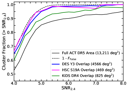
Figure 15: The fraction of ACT DR5 cluster candidates that are optically confirmed as clusters (with a redshift measurement) as a function of SNR_2.4, broken down according to overlap with the indicated deep optical surveys (colored solid lines). Objects that are not confirmed clusters may be contaminating false positives (e.g., noise fluctuations in the maps) or genuine high-redshift systems that are not yet optically confirmed. The dashed line (labeled $1-F_{\rm False}$) shows the expected purity of the cluster sample, based on a simulation of the survey (see Section 2.2 and Fig. 6). The small difference between $1-F_{\rm False}$ and the tracks for the DES Y3 and HSC regions indicates that the optical follow-up is essentially complete for these parts of the sky. However, the difference between $1-F_{\rm False}$ and the full ACT DR5 survey footprint indicates the potential for further follow-up to add up to 960 clusters to the sample.

4 The ACT DR5 Cluster Catalog

4.1 Properties of the Cluster Catalog

This release of the ACT cluster catalog consists of 4195 optically confirmed galaxy clusters detected with SNR $>4$ using the combination of the 98 and 150 GHz ACT maps. Table 1 describes the data provided in the catalog. Each cluster in the catalog has a redshift measurement (see Section 3.1) and a set of mass estimates inferred from our SZ observable, $\tilde{y}_{0}$ (see Section 2.3). The left panel of Fig. 16 summarizes the contents of the catalog by showing the distribution of the clusters in terms of co-moving coordinates in the celestial equatorial plane (i.e., right ascension is used as the angular coordinate). The right panel of Fig. 16 shows a similar plot but in spherical polar coordinates.

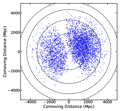
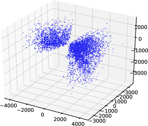
Figure 16: The left panel displays a wedge plot showing the contents of the ACT DR5 cluster catalog, drawn in the equatorial plane. Right Ascension is used as the angular coordinate, with 0^∘ RA pointing to the right from the origin, and increasing anticlockwise. The radial coordinate is co-moving distance in Mpc. Each point represents a cluster in the catalog, with the size of each point scaling with cluster mass. The dashed circles mark the distances equivalent to redshifts 0.5, 1.0, 1.5, and 2.0, starting from the observer’s location at (0, 0). The larger number of clusters seen on the right of the plot compared to the left reflects the fact that ACT surveyed much more sky area at those RA coordinates (see Fig. 1). The right panel shows a 3d projection of the same information in spherical polar coordinates; here the axes are comoving distance in Mpc.

Several studies have found evidence that cluster masses calibrated against the Arnaud et al. (2010) scaling relation, our fiducial mass estimate (labelled $M^{\rm UPP}_{\rm 500c}$ in this work), are lower than those measured from weak lensing (e.g, von der Linden et al., 2014; Hoekstra et al., 2015; Battaglia et al., 2016; Miyatake et al., 2019). For this reason, we provide a set of mass estimates that have been re-scaled according to a richness-based weak-lensing mass calibration, following a similar procedure to that described in Hilton et al. (2018).

Using the sample of 383 SNR${}_{2.4}>6$ clusters (expected to be $>98$% pure; see Section 3.3) with $\lambda$ measurements from redMaPPer in the DES Y3 footprint, and the McClintock et al. (2019) $\lambda$–mass relation, we find that the ratio of the average A10–calibrated SZ-mass to the average richness-based, weak-lensing calibrated mass is $\langle M^{\rm UPP}_{\rm 500c}\rangle/\langle M^{\rm\lambda WL}_{\rm 500c}\rangle=0.71\pm 0.07$. Masses that have been rescaled according to this calibration factor are labelled $M^{\rm Cal}_{\rm 500c}$ throughout this work, and for convenience are provided in the cluster catalog (see Table 1). This calibration factor is in good agreement with the value reported in Hilton et al. (2018), which used SDSS redMaPPer $\lambda$ measurements and the Simet et al. (2017) $\lambda$–mass relation. However, if we use the redMaPPer SDSS $\lambda$ measurements and the Simet et al. (2017) relation (instead of the McClintock et al. (2019) relation) with the ACT DR5 $M^{\rm UPP}_{\rm 500c}$ estimates, then we find $\langle M^{\rm UPP}_{\rm 500c}\rangle/\langle M^{\rm\lambda WL}_{\rm 500c}\rangle=0.66\pm 0.08$.

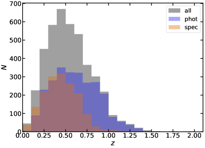
Figure 17: Redshift distribution of the ACT DR5 cluster sample. The sample spans the redshift range $0.04{}<z<1.91{}$ (median $z=0.52{}$). The distribution split according to redshift type (spectroscopic or photometric) is also shown; 39.3% of the clusters in the sample have spectroscopic redshifts.

We present the redshift distribution of the cluster sample in Fig. 17. The sample has median $z=0.52{}$, similar to other SZ-selected samples (e.g., Hilton et al., 2018; Bocquet et al., 2019; Bleem et al., 2020) and covers the redshift range $0.04{}<z<1.91{}$. Largely due to the overlap with SDSS, a significant fraction of the redshifts are spectroscopic (39.3%). The highest redshift cluster in the sample, ACT-CL J0217.7-0345, is detected with SNR${}_{2.4}=5.7$, and was first reported as the $z=1.91^{+0.19}_{-0.21}$ X-ray selected cluster XLSSU J021744.1-034536 by Willis et al. (2013b). It is also the highest redshift SZ detected cluster currently known (Mantz et al., 2014, 2018). The catalog contains 222 $z>1$ clusters, which is greater than the total number of clusters reported in the previous ACT cluster catalog (Hilton et al., 2018). Most of the clusters in the catalog have previously been detected in other surveys; here we report 868 new cluster discoveries, with median $z=0.75{}$. This figure excludes clusters detected in the redMaPPer DES Y3 and CAMIRA S19A catalogs.

Fig. 18 shows the ACT DR5 sample in the (mass, redshift) plane, in comparison with other SZ-selected cluster samples from Planck (Planck Collaboration et al., 2016b) and SPT (Bocquet et al., 2019; Bleem et al., 2020; Huang et al., 2020a). Here we show the richness-based weak-lensing calibrated masses from ACT ($M^{\rm Cal}_{\rm 500c}$), as these are on a similar mass scale to SPT (see Section 5.1 below). We plot both the full ACT DR5 sample down to SNR $>4$ (shown as the small blue points) and a subsample with a cut of SNR${}_{2.4}>5$ applied, which is closer to the detection thresholds used in the other surveys, and more closely resembles the sample that will be used for future cosmological analyses. The ACT DR5 sample contains more clusters than all of the previous blind SZ cluster searches combined. Due to the higher spatial resolution of the instruments, both the ACT DR5 and SPT samples reach to significantly lower mass limits than the PSZ2 catalog for $z>0.2$. As Fig. 18 shows, the SPTpol sample (Huang et al., 2020a) is more sensitive to lower mass clusters than ACT DR5 when a similar detection threshold is applied, although this survey covers only 94 deg².

Inspection of Fig. 18 suggests that there may be a deficit of clusters in the redshift range $1<z<1.1$. This is extremely unlikely to be a real feature, and may arise due to a bias in the photometric redshifts. We will investigate this further with future spectroscopic follow-up of such high redshift systems.

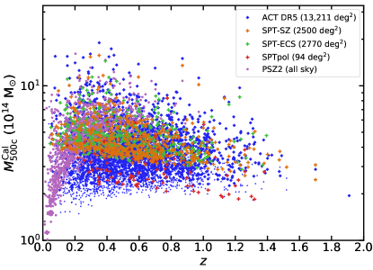
Figure 18: Comparison of the ACT DR5 cluster sample in the (mass, redshift) plane with other blind SZ surveys: PSZ2 (Planck Collaboration et al., 2016b), SPT-SZ (Bocquet et al., 2019), SPT-ECS (Bleem et al., 2020), and SPTpol (Huang et al., 2020a). The large blue points show the ACT DR5 sample selected with SNR${}_{2.4}>5$, which is similar to the detection thresholds used in the other surveys. The small blue points extend this to include the full ACT DR5 sample. The ACT DR5 SZ masses displayed here have been rescaled according to a richness-based weak-lensing mass calibration, which is a close match to the SPT mass scale (see Section 5.1). Mass measurements from the SPT surveys and PSZ2 are as reported in the respective catalogs. The ACT DR5 sample has been plotted behind the other surveys to aid clarity.

4.2 Comparison with the ACT DR3 Cluster Catalog

As discussed extensively in Choi et al. (2020) and Aiola et al. (2020), there have been many changes to the ACT data processing pipelines at all levels of the analysis since the data release that the Hilton et al. (2018) ACTPol cluster catalog (ACT DR3 hereafter) is based on. In this work, we have used maps produced using a new co-adding procedure that incorporates data from all observing seasons and, for the first time, includes data taken during the day time (N20). As noted in Section 2.1, these co-added maps include preliminary data from the 2017 and 2018 observing seasons that have not been subjected to the full battery of tests as used in the CMB power spectrum analysis presented in Choi et al. (2020) and Aiola et al. (2020). In this work we also use a different, multi-frequency matched filter approach in the cluster finder compared to the algorithm described in Hilton et al. (2018).

We begin by checking the recovery of ACT DR3 clusters in the ACT DR5 catalog. Hilton et al. (2018) reported the detection of 182 SNR $>4$ clusters, of which 175/182 are within the ACT DR5 cluster search area (i.e., 7 clusters fall within regions masked in DR5). Of these, 154/175 are recovered within 2.5′ of the position of a candidate in the ACT DR5 catalog, leaving 21 clusters that are not detected at SNR $>4$. The missing 21 clusters have median SNR$~{}=4.3$ in the ACT DR3 catalog, although three SNR $>5$ clusters (ACT-CL J0238.2+0245, ACT-CL J0341.9+0105, and ACT-CL J2337.6-0856) are not detected in the ACT DR5 catalog. Half of the missing 21 clusters were previously reported in other catalogs (Goto et al., 2002; Lopes et al., 2004; Durret et al., 2011; Menanteau et al., 2013b; Rykoff et al., 2014; Wen & Han, 2015). Re-running the ACT DR5 cluster search with a lower detection threshold recovers 13/21 of the missing ACT DR3 clusters at SNR $>3$.

Fig. 19 presents a comparison of the ACT DR3 mass estimates reported in Hilton et al. (2018) with the new measurements from ACT DR5. We highlight the objects detected with SNR${}_{2.4}>6$ in both samples, as these should not be affected by filter noise bias at any significant level. As expected, both sets of measurements follow a tight correlation. However, we see that the ACT DR5 masses are on average systematically $\approx 7$% lower than the ACT DR3 measurements. We have verified that the difference in the filtering approach between Hilton et al. (2018) and this work is not the cause (consistent $\tilde{y}_{0}$ measurements are obtained when running either method on the same map). It may be the case that scale-dependent bandpass effects (see Madhavacheril et al., 2020), which are not accounted for in this analysis, could explain part of the offset. While we have not yet been able to resolve this discrepancy, we note that gain errors at the level of a few per cent are expected in the co-added maps analysed in this work (N20). Therefore, we caution users of the ACT DR5 cluster catalog that the $\tilde{y}_{0}$ measurements reported here (and in turn the $M^{\rm UPP}_{\rm 500c}$ masses) may be systematically underestimated by $\approx 5-10$%, if the ACT DR3 catalog is taken as “truth”. This should be kept in mind when comparing these values against external catalogs. However, mass calibration against external datasets can still be used to absorb any systematic calibration error (as should be the case for the $M^{\rm Cal}_{\rm 500c}$ mass estimates).

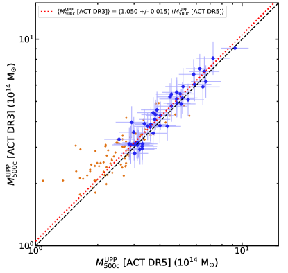
Figure 19: Comparison between ACT DR5 mass estimates (this work, plotted along the horizontal axis) and previous ACT cluster mass estimates as reported in Hilton et al. (2018) (labeled ACT DR3). Both analyses assume the same scaling relation between SZ signal and mass. The large blue points are objects with SNR${}_{2.4}>6$ in both samples (for which the unweighted mean ratio is calculated, shown by the dotted red line), while the small orange points (without error bars) show objects below this threshold. The dashed black line shows the 1:1 correlation.

5 Discussion

5.1 The SZ Cluster Mass Scale

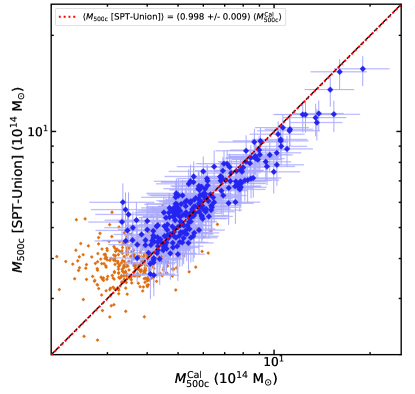
Figure 20: Comparison between ACT DR5 mass estimates rescaled according to a richness-based weak-lensing mass calibration ($M^{\rm Cal}_{\rm 500c}$; Section 4) with SPT masses reported in Bocquet et al. (2019), Bleem et al. (2020), and Huang et al. (2020a). The large blue points are objects with signal-to-noise $>6$ in both ACT and SPT (for which the unweighted mean ratio is calculated, shown by the dotted red line), while the small orange points (without error bars) show objects below this threshold. The dashed black line shows the 1:1 correlation.

Mass calibration of cluster samples is the key systematic that limits their ability to constrain cosmological parameters and is a topic of much debate in the literature (e.g., von der Linden et al., 2014; Hoekstra et al., 2015; Planck Collaboration et al., 2016a; Battaglia et al., 2016; Smith et al., 2016; Medezinski et al., 2018; Miyatake et al., 2019). Cluster mass estimation based on any kind of data is dependent upon a number of assumptions. Here we present a simple comparison of the mass estimates available in the ACT DR5 catalog with previous SZ surveys, and a compendium of weak-lensing mass estimates (CoMaLit; Sereno, 2015), as an illustration of how they may be used. Future works based on the ACT DR5 catalog will investigate this topic in much more detail.

In Hilton et al. (2018), we presented comparisons between ACT cluster mass estimates and the SPT-SZ and PSZ2 catalogs. While we found excellent agreement with the Bleem et al. (2015b) SPT-SZ catalog, we noted an apparent mass-dependent trend when comparing the ACT masses with PSZ2 (although at low significance). This was identified in a plot of the ACT–PSZ2 mass ratio versus the ACT mass estimate. We subsequently found that the apparent mass-dependent trend was an illusion driven by the combination of a regrettable choice in the plot axes (i.e., plotting the ACT mass instead of the PSZ2 mass as the independent coordinate), the very different selection of the ACT and PSZ2 cluster samples (PSZ2 detects $z<0.2$ clusters at high significance down to low masses while ACT does not, and the reverse is true at higher $z$), and that the measurements themselves are subject to a significant amount of scatter, especially at low signal-to-noise. We rectify this in the comparisons presented here by simply plotting the mass estimates in each catalog against each other.

Fig. 20 shows a comparison between the ACT DR5 masses rescaled using the richness-based weak-lensing mass calibration (see Section 4) against a union of the SPT cluster catalogs (Bocquet et al. 2019; Bleem et al. 2020; Huang et al. 2020a; note that we make no attempt to remove duplicate objects). This ‘SPT-Union’ sample contains 618 clusters in common with ACT DR5 (326 from SPT-SZ, 266 from SPT-ECS, and 26 from SPTpol), if we include all objects down to the detection thresholds used by each survey. The masses are clearly correlated, although there is a tendency for the ACT mass estimates to be slightly larger than those from SPT, particularly at the high mass end.

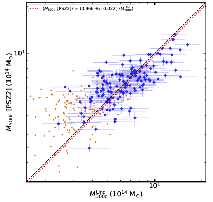
Figure 21: Comparison between ACT DR5 mass estimates, uncorrected for bias due to the steepness of the cluster mass functon ($M^{\rm Unc}_{\rm 500c}$; Section 4), with PSZ2 masses reported in Planck Collaboration et al. (2016b). The large blue points highlight objects with signal-to-noise $>6$ in both surveys, while the small orange points (without error bars) show objects below this threshold. The lines have the same meaning as in Fig. 20.

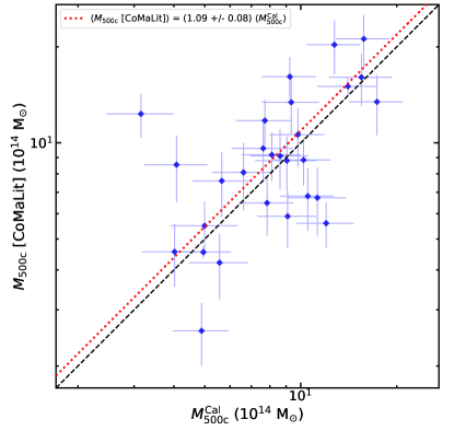
Figure 22: Comparison between ACT DR5 mass estimates rescaled according to a richness-based weak-lensing mass calibration ($M^{\rm Cal}_{\rm 500c}$; Section 4) with weak-lensing masses from the CoMaLit database (Sereno, 2015). Here we use the LC²-single catalog from CoMaLit, which consists of objects modeled using a single halo, and we restrict the selection to include only clusters with weak-lensing mass estimates with $<25\%$ uncertainties. The lines have the same meaning as in Fig. 20.

Leaving aside any question of mass-dependent scaling for future work, we can make a simple assessment of the overall consistency of the mass scale between the two samples using the unweighted mean ratio of their masses (e.g., Sifón et al., 2016; Hilton et al., 2018). Here we use the 254 objects detected at signal-to-noise$~{}>6$ in both samples, as $>98$% of the ACT DR5 candidates with SNR${}_{2.4}>6$ were confirmed to be clusters in the DES Y3 and HSC S19A regions (see Section 3.3). Using a high signal-to-noise threshold also mitigates the effect of the ‘noise floor’ in the case of a significant difference in depth between two samples (although that is not the case for the comparison here). We find $\langle M_{\rm 500c}\left[\rm SPT\mathchar 45\relax Union\right]\rangle=(0.998\pm 0.009)\,\langle M^{\rm Cal}_{\rm 500c}\rangle$, where the uncertainty is the standard error on the mean (note that this does not account for the uncertainty on the richness-based weak-lensing mass calibration factor itself). We find results that are consistent with this if we compare ACT DR5 against the individual SPT catalogs: $\langle M_{\rm 500c}\left[\rm SPT\mathchar 45\relax SZ\right]\rangle=(1.027\pm 0.012)\,\langle M^{\rm Cal}_{\rm 500c}\rangle$; $\langle M_{\rm 500c}\left[\rm SPT\mathchar 45\relax ECS\right]\rangle=(0.961\pm 0.014)\,\langle M^{\rm Cal}_{\rm 500c}\rangle$; and $\langle M_{\rm 500c}\left[\rm SPTpol\right]\rangle=(1.001\pm 0.027)\,\langle M^{\rm Cal}_{\rm 500c}\rangle$. Similarly to Hilton et al. (2018), we see that despite the differences between how the ACT DR5 and SPT samples were constructed, and the very different method used to calibrate the mass estimates, the richness-based weak-lensing calibrated masses are on a similar mass scale to SPT.

Fig. 21 presents a similar comparison between ACT DR5 and the PSZ2 catalog (Planck Collaboration et al., 2016b). Since we adopted the same fiducial X-ray calibrated mass scaling relation from A10 as used in the PSZ2 catalog, we would expect the ACT DR5 clusters to follow the same mass scale. Here the comparison is made against ACT DR5 mass estimates that neglect the bias correction that accounts for the steepness of the cluster mass function, as such a correction is not applied to the masses reported in the PSZ2 catalog (see Section 2.3 and the discussion in Battaglia et al., 2016). We use a 5′ radius to cross-match the two catalogs, resulting in a sample of 327 clusters, if we include all objects down to the detection threshold of each survey. As shown in Fig. 21, the scatter between the PSZ2 and ACT DR5 masses is large, but the mass scale is indeed similar: we find $\langle M_{\rm 500c}\left[\rm PSZ2\right]\rangle=(0.966\pm 0.022)\,\langle M^{\rm Unc}_{\rm 500c}\rangle$ from the 148 objects detected with signal-to-noise$~{}>6$ in both catalogs.

Table 3: Strong Lens Catalogs

Code	Reference
M16	More et al. (2016)
D17	Diehl et al. (2017)
S18	Sonnenfeld et al. (2018)
W18	Wong et al. (2018)
P19	Petrillo et al. (2019)
J19	Jacobs et al. (2019a)
J19a	Jacobs et al. (2019b)
H20a	Huang et al. (2020b)
H20b	Huang et al. (2020c)
Jae20	Jaelani et al. (2020)
D20	Diehl et al. (2020)

Note. — Entries in the knownLensRefCode column of the cluster catalog (see Table 1) correspond to the Code column used here.

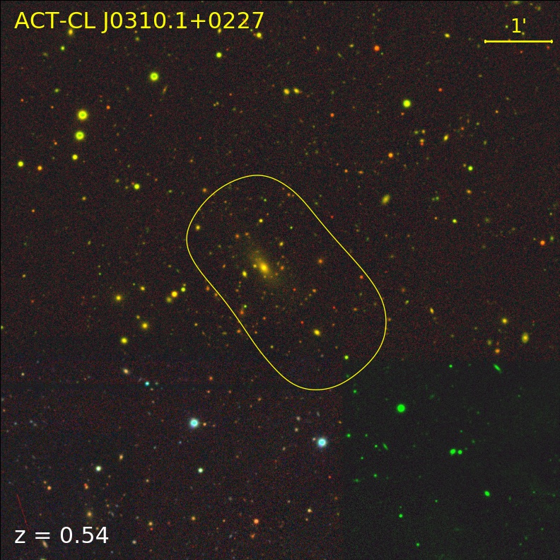
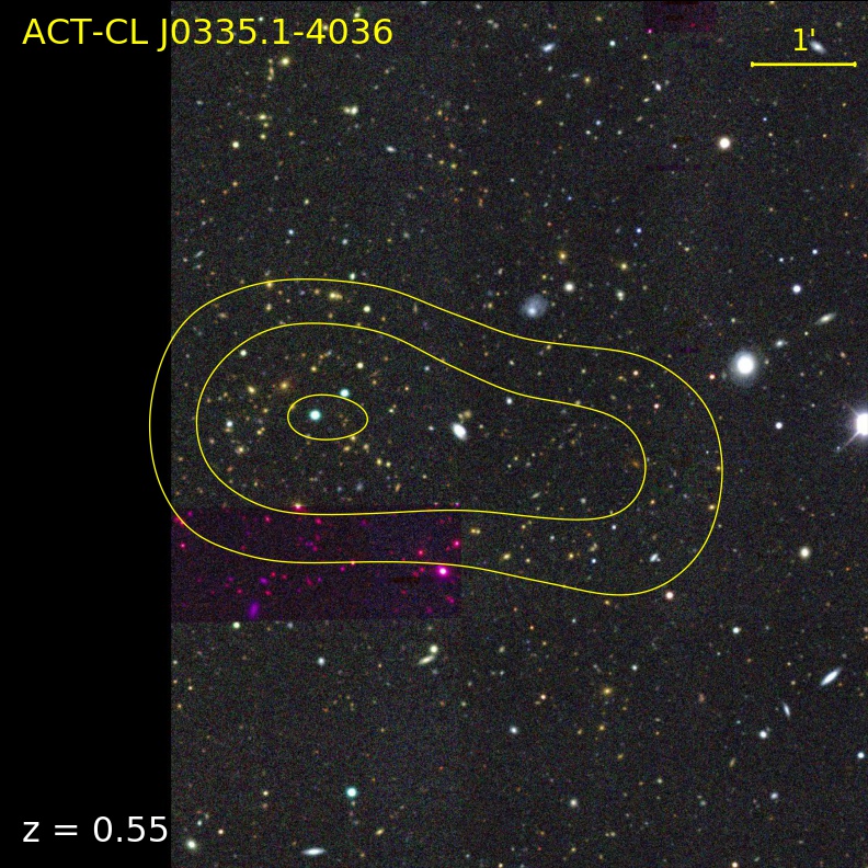
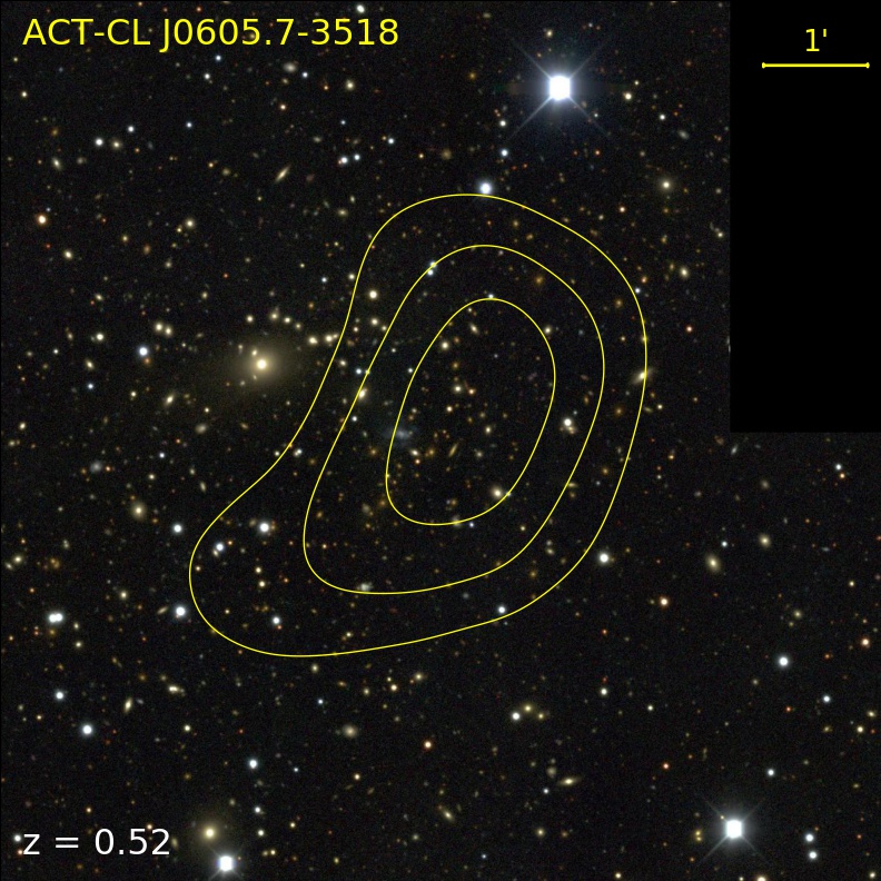
Figure 23: Examples of possible projected systems (see Section 5.2.1). Each image is 8′ on a side, with North at the top, East at the left. See Fig. 10 for an explanation of the contour levels.

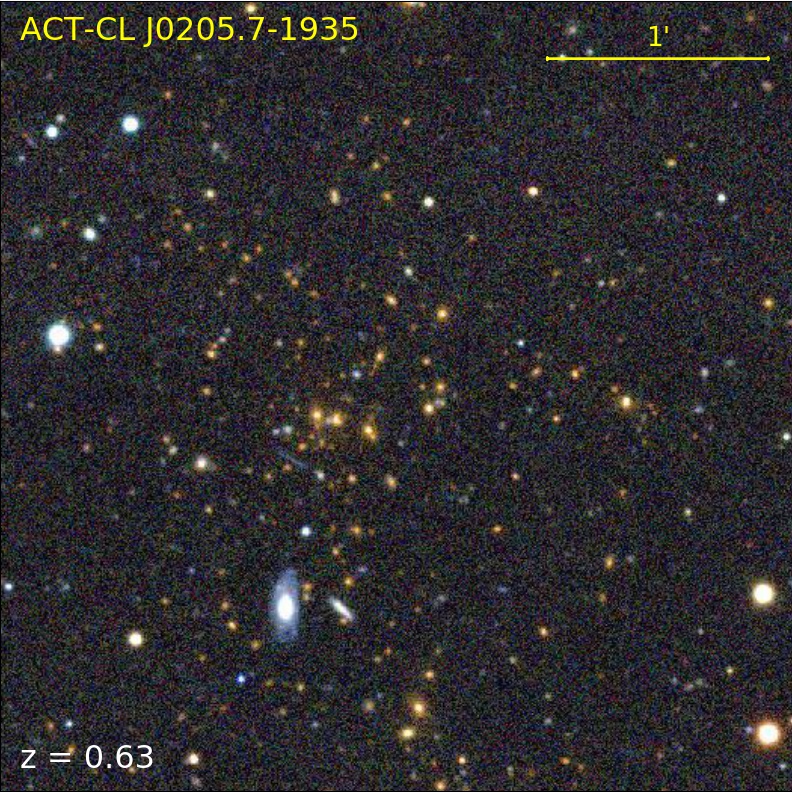
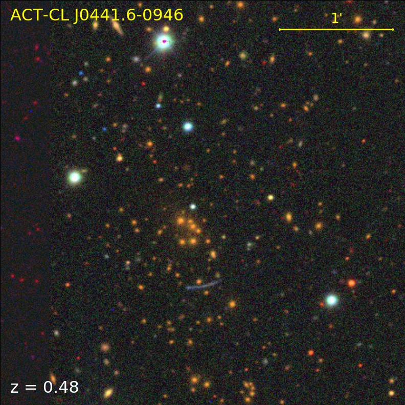
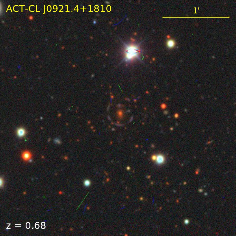
Figure 24: Examples of systems that show possible strong gravitational lensing features (see Section 5.2.2). ACT-CL J0205.7-1935 contains a lens candidate in the Diehl et al. (2020) catalog; ACT-CL J0441.6-0946 contains the known lens DESI-070.4130-09.7774 (Huang et al., 2020c); and the lens in ACT-CL J0921.4+1810 appears to be identified for the first time in this work. Each image is 3.5′ on a side, with North at the top and East at the left.

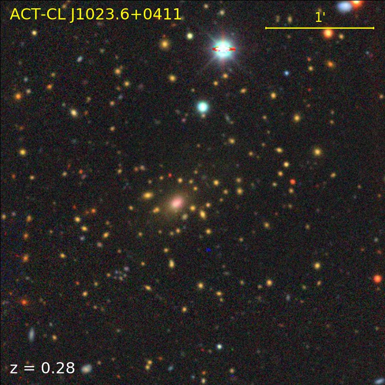
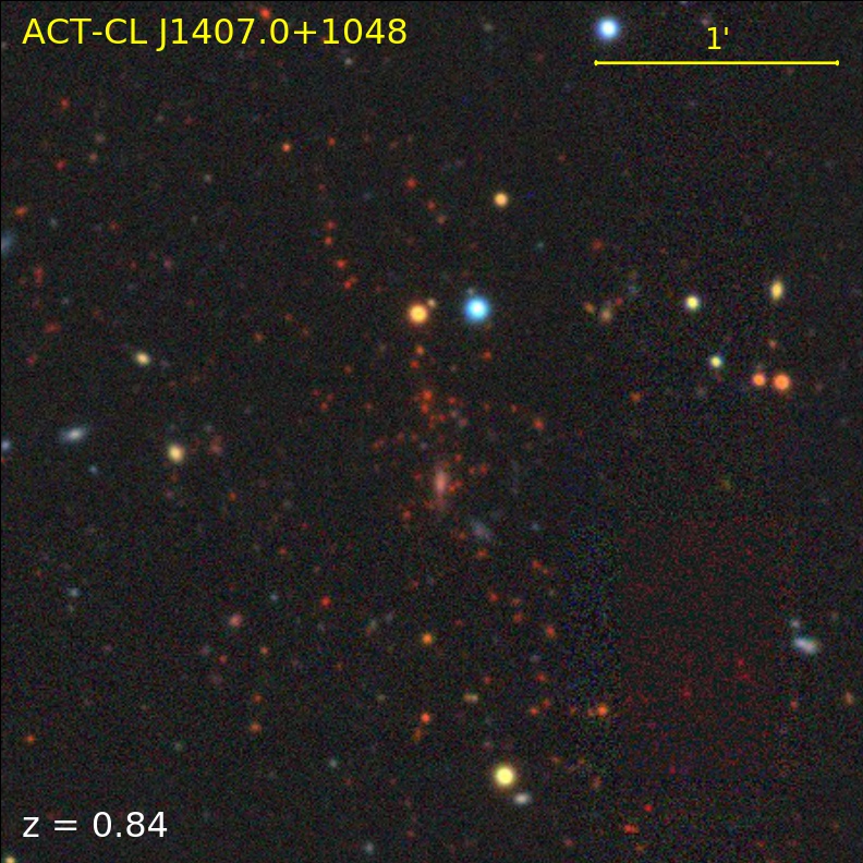
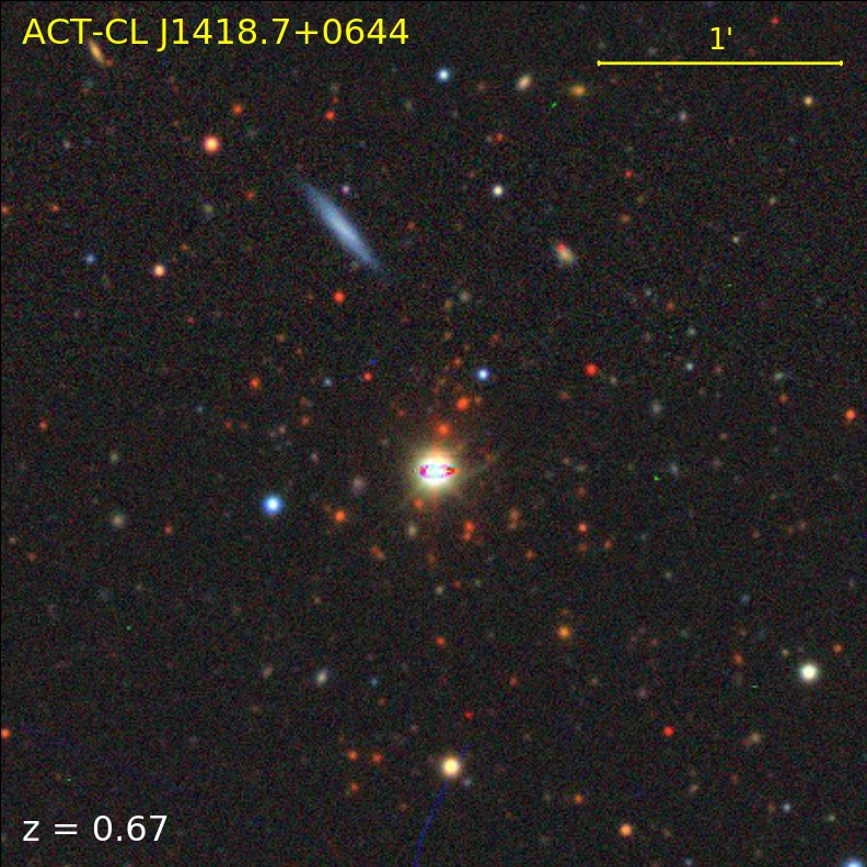
Figure 25: Examples of systems with activity in the cluster core (star formation or possible AGNs; see Section 5.2.3). Each image is 3.5′ on a side, with North at the top and East at the left. ACT-CL J1023.6+0411 is the well known $z=0.29$ cool core ZwCl 3146 cluster; ACT-CL J1407.0+1048 is the second ranked cluster in the sample at $z>0.8$ in terms of SNR, and perhaps has a starburst galaxy in its core; ACT-CL J1418.7+0644 is a high significance detection by ACT, but was previously rejected as a false detection in the X-ray cluster catalog of Vikhlinin et al. (1998).

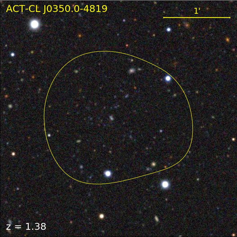
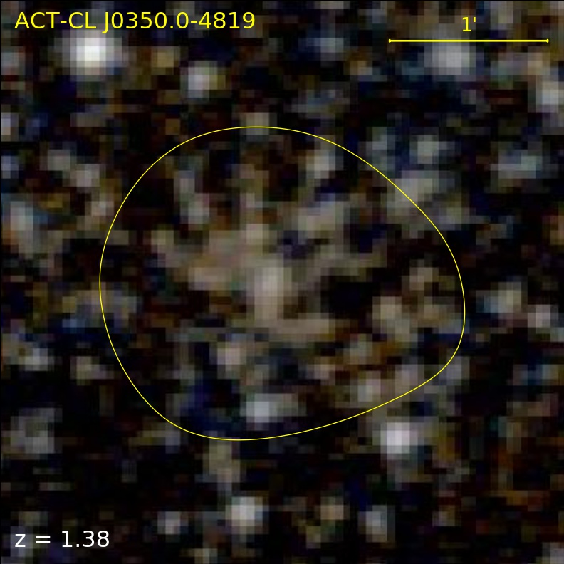
Figure 26: The newly discovered high redshift cluster ACT-CL J0350.0-4819 at $z=1.38$. The left panel shows the DES Y3 $gri$ optical image, which shows a striking number of blue galaxies within the yellow SZ signal-to-noise contour. The right panel shows the WISE IR imaging, demonstrating that the cluster itself is a genuine high redshift system.

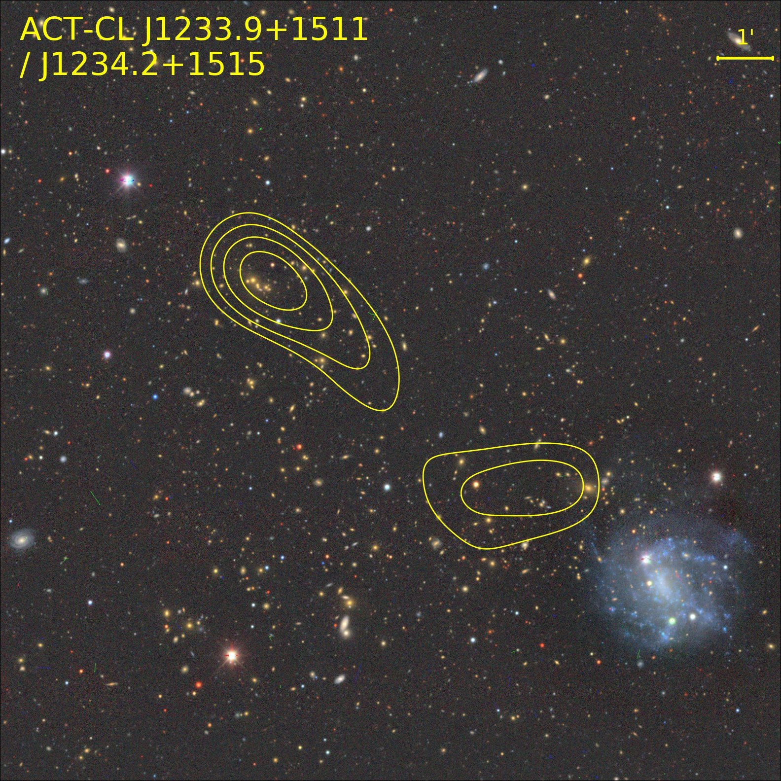
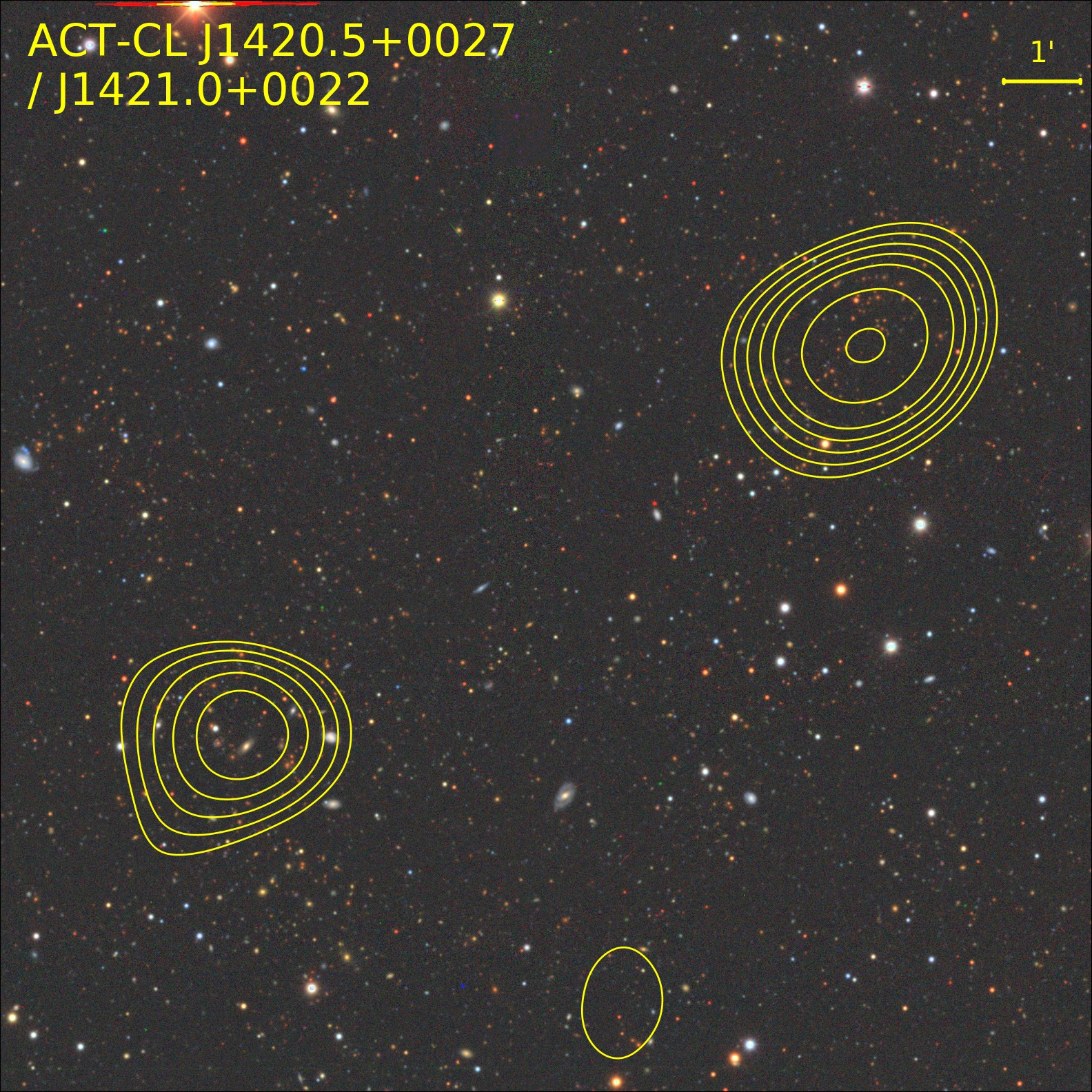
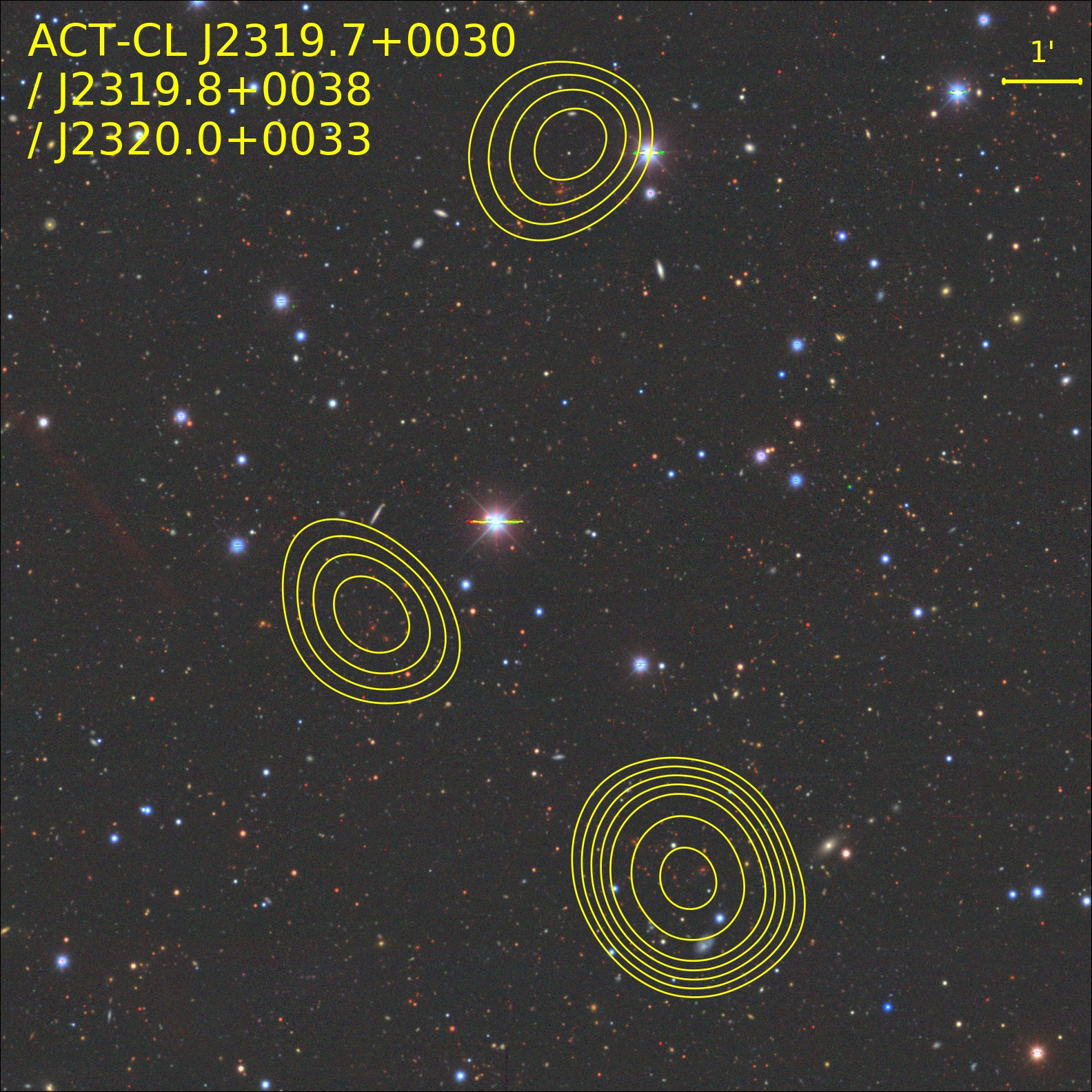
Figure 27: Example DECaLS $grz$ images of multiple systems (see Section 5.2.5): ACT-CL J1233.9+1511/J1234.2+1515 at $z=0.29$ (possibly a pre- or post-merger system); ACT-CL J1420.5+0027/J1421.0+0022 at $z=0.64$ (two clusters separated by 3.6 Mpc); and the $z=0.90$ triple system ACT-CL J2319.7+0030/J2319.8+0038/J2320.0+0033 (the RCS2 supercluster; Gilbank et al., 2008). Each image is 13′ on a side, with North at the top, East at the left. The lowest contour level shown corresponds to 3$\sigma$ significance in the filtered ACT map. The difference between levels increases by 0.5$\sigma$ ($3<$ SNR $<5$), 1$\sigma$ ($5<$ SNR $<10$), and 2$\sigma$ ($10<$ SNR $<20$).

As an independent check of the richness-based weak-lensing mass calibration used in this work, Fig. 22 presents a comparison with a heterogeneous database of weak-lensing masses assembled from the literature (Sereno, 2015). Even though the comparison is made only with clusters that have $<25$% uncertainty in the weak-lensing masses, the scatter is large. Nevertheless, the overall mass scale is consistent with the richness-based weak-lensing calibration derived from DES observations; $\langle M_{\rm 500c}\left[\rm CoMaLit\right]\rangle=(1.09\pm 0.08)\,\langle M^{\rm Cal}_{\rm 500c}\rangle$. Future work will explore the mass calibration of the ACT DR5 sample using optical weak-lensing data from DES, HSC-SSP, and KiDS, as well as from gravitational lensing of the CMB.

5.2 Notable Clusters

In this Section we briefly discuss a few notable categories of systems that may be of interest for future studies. This list is not meant to be comprehensive, and results for the most part from visual inspection of the cluster catalog using the available optical/IR data (see Section 3.2). Further possible examples besides those mentioned here may be found by inspecting the notes and warnings columns of the cluster catalog (see Table 1).

5.2.1 Projected Systems

During visual inspection of the cluster candidates, we identified 46 systems that may be projections of two or more clusters at different redshifts. These are indicated in the warnings field of the cluster catalog (see Table 1). Fig. 23 shows a few examples. One of these cases (ACT-CL J0335.1-4036) is clearly a blended SZ detection of two systems, which the cluster finder has failed to separate because all of the pixels in both systems are well above our detection threshold. We will seek to improve the object deblending for future cluster catalog releases.

5.2.2 Strong Lensing Systems

A search of the literature shows that there are 210 known strong gravitational lenses located within 2 Mpc projected distance of clusters in the ACT DR5 release, as recorded in the knownLens field of the cluster catalog (see Table 1). Table 3 lists the lens catalogs that were searched and the corresponding code used in the knownLensRefCode in the cluster catalog. We also identified a further 67 clusters that show possible strong lensing features, based on visual inspection of the available optical imaging. These are indicated in the notes field of the cluster catalog. Fig. 24 shows some examples of both known lenses and new candidates.

5.2.3 Systems With Active or Star Forming Central Galaxies

We flagged 14 systems as potentially hosting central AGNs or significant star formation, purely on the basis of their appearance in the available optical/IR imaging, including the well known cool core cluster ZwCl 3146 (ACT-CL J1023.6+0411) at $z=0.29$ (e.g., Romero et al., 2020). One of our highest significance detections at $z>0.8$ is a new cluster in this category, ACT-CL J1407.0+1048 ($z=0.84$, SNR${}_{2.4}=33.8$, $M^{\rm Cal}_{500c}=(9.1^{+1.7}_{-1.5})\times 10^{14}$ $M_{\sun}$), which has a blue BCG as shown in the DECaLS image (Fig. 25). This cluster may have similar properties to the Phoenix cluster (McDonald et al., 2012), but follow-up at other wavelengths is needed to confirm this. Some objects in this category may be “quasars masquerading as clusters” as identified at X-ray wavelengths (Somboonpanyakul et al., 2018; Donahue et al., 2020), following further investigation. For example, ACT-CL J1418.7+0644 (pictured in Fig. 25) is detected with SNR${}_{2.4}=12.7$ in the ACT DR5 catalog, but was rejected as a false detection in the X-ray cluster catalog of Vikhlinin et al. (1998).

5.2.4 A Blue High Redshift Galaxy Cluster?

Fig. 26 shows optical and WISE IR imaging of the newly discovered $z=1.38$ cluster ACT-CL J0350.0-4819. The photometric redshift of this system was determined using DECaLS photometry (see Section 3.1.4), and we lack any spectroscopic information. Nevertheless, there is an apparent overdensity of galaxies with blue colors at the cluster position, as seen in the DES $gri$ optical image. If this is not simply projection along the line of sight, then it may be that this system hosts an unusually large number of star forming galaxies. We intend to obtain follow-up spectroscopy of this system to determine if this is in fact the case. ACT-CL J0350.0-4819 is also detected by the Wavelet Z Photometric optical cluster finding algorithm (WaZP; Aguena et al. 2020 presents a catalog based on DES Y1), in a preliminary search of the DES Y6 data. WaZP does not assume a red-sequence model and searches for clusters as spatial overdensities using photometric redshifts.

5.2.5 Multiple Systems

We conducted a search for pairs or groups of clusters in the catalog that may be physically associated. These objects may be of interest for those studying cluster mergers, filaments/large scale structure around clusters, and superclusters. We select candidates for this category as objects that have a neighbouring SZ source within a projected distance of 10 Mpc, and a peculiar velocity difference of $<5000$ km s^-1. We find a total of 160 such systems, consisting of 144 pairs, 15 triples, and 1 quadruple system, which are listed in Table 4. Note, however, that some clusters are part of more than one system (e.g., the $z=0.49$ triple system ACT-CL J0059.6+1310/J0059.8+1344/J0059.9+1319 is also listed as the pairs ACT-CL J0059.6+1310/J0059.9+1319 and ACT-CL J0059.8+1344/J0059.9+1319). We also include objects with photometric redshifts in this search, but flag these in the catalog, since the uncertainties on these redshifts are much larger than spectroscopic redshift errors.

Table 4: Systems of Multiple SZ Sources

Name	Mean $z$	Separation	Photo-$z$?
		(Mpc)
ACT-CL J0000.7$+$0225
/J2359.5$+$0208	0.43	8.1	$\cdots$
ACT-CL J0003.0$-$3520
/J0003.8$-$3517	0.76	4.1	✓
ACT-CL J0005.0$+$0212
/J0005.7$+$0222	0.84	7.0	✓
ACT-CL J0018.3$+$1618
/J0018.5$+$1626	0.55	3.3	$\cdots$
ACT-CL J0019.6$+$0336
/J0020.0$+$0351	0.27	4.0	✓

Note. — Only a subset of the available fields in this catalog are shown here. Table 4 is published in its entirety in machine-readable format. A portion is shown here for guidance regarding its form and content.

We find multiple systems across the redshift range $0.04<z<1.2$ (median $z=0.42)$, and the average maximum projected separation between the components of these systems is 5.8 Mpc. Fig. 27 shows a few examples. Due to the increased depth of the ACT DR5 maps, we now detect all three components of the $z=0.9$ RCS2 supercluster (Gilbank et al., 2008, recorded here as ACT-CL J2319.7+0030/J2319.8+0038/J2320.0+0033). Some of these systems may be pre or post-merger systems (e.g., ACT-CL J1233.9+1511/J1234.2+1515 at $z=0.29$, shown in Fig. 27).

6 Summary

This work presents the first cluster catalog derived from 98 and 150 GHz observations with the AdvACT receiver, covering a search area of 13,211 deg². The catalog contains 4195 optically confirmed galaxy clusters with redshift and mass estimates, making it the largest SZ-selected cluster catalog to date. It is more than 22 times larger than the previous ACT cluster catalog (Hilton et al., 2018), illustrating the huge gains in sensitivity and survey speed achieved by the upgraded AdvACT receiver (Henderson et al., 2016). Assuming a relation between SZ-signal and mass calibrated from X-ray observations (Arnaud et al., 2010), the 90% completeness limit of the survey for SNR${}_{2.4}>5$ is $M_{\rm 500c}>3.8{}\times 10^{14}\,M_{\sun}$.

Thanks to the overlap with deep and wide optical surveys like DES (Abbott et al., 2018), DECaLS (Dey et al., 2019), HSC-SSP (Aihara et al., 2018), KiDS (Wright et al., 2019), and SDSS (Ahumada et al., 2020), the optical follow-up of the survey is complete over much of the survey area. The cluster sample has median $z=0.52{}$ and covers the redshift range $0.04{}<z<1.91{}$, with 222 $z>1$ systems, and 868 newly discovered clusters. In the regions that overlap with DES Y3, HSC S19A, and KiDS DR4, $95-98$% of the candidates detected with SNR${}_{2.4}>6$ have been confirmed as clusters.

The cluster and source detection package developed for this work is capable of analysing the next generation of deep, wide multi-frequency mm-wave maps that will be produced by experiments such as the Simons Observatory (Ade et al., 2019). It will be made publicly available at https://github.com/simonsobs/nemo/ and on the Python Package Index (PyPI) under a free software license.

References

- Abbott et al. (2018) Abbott, T. M. C., Abdalla, F. B., Allam, S., et al. 2018, ApJS, 239, 18, doi: 10.3847/1538-4365/aae9f0
- Abell et al. (1989) Abell, G. O., Corwin, Harold G., J., & Olowin, R. P. 1989, ApJS, 70, 1, doi: 10.1086/191333
- Ade et al. (2019) Ade, P., Aguirre, J., Ahmed, Z., et al. 2019, J. Cosmology Astropart. Phys, 2019, 056, doi: 10.1088/1475-7516/2019/02/056
- Aguena et al. (2020) Aguena, M., et al. 2020, in preparation, 000. https://arxiv.org/abs/TBC
- Ahumada et al. (2020) Ahumada, R., Allende Prieto, C., Almeida, A., et al. 2020, ApJS, 249, 3, doi: 10.3847/1538-4365/ab929e
- Aihara et al. (2018) Aihara, H., Arimoto, N., Armstrong, R., et al. 2018, PASJ, 70, S4, doi: 10.1093/pasj/psx066
- Aiola et al. (2020) Aiola, S., Calabrese, E., Maurin, L., et al. 2020, arXiv e-prints, arXiv:2007.07288. https://arxiv.org/abs/2007.07288
- Allen et al. (2008) Allen, S. W., Rapetti, D. A., Schmidt, R. W., et al. 2008, MNRAS, 383, 879, doi: 10.1111/j.1365-2966.2007.12610.x
- Allen et al. (2004) Allen, S. W., Schmidt, R. W., Ebeling, H., Fabian, A. C., & van Speybroeck, L. 2004, MNRAS, 353, 457, doi: 10.1111/j.1365-2966.2004.08080.x
- Ansarinejad et al. (2020) Ansarinejad, B., et al. 2020, in preparation, 000. https://arxiv.org/abs/TBC
- Arnaud et al. (2005) Arnaud, M., Pointecouteau, E., & Pratt, G. W. 2005, A&A, 441, 893, doi: 10.1051/0004-6361:20052856
- Arnaud et al. (2010) Arnaud, M., Pratt, G. W., Piffaretti, R., et al. 2010, A&A, 517, A92, doi: 10.1051/0004-6361/200913416
- Astropy Collaboration et al. (2013) Astropy Collaboration, Robitaille, T. P., Tollerud, E. J., et al. 2013, A&A, 558, A33, doi: 10.1051/0004-6361/201322068
- Barkhouse et al. (2006) Barkhouse, W. A., Green, P. J., Vikhlinin, A., et al. 2006, ApJ, 645, 955, doi: 10.1086/504457
- Battaglia et al. (2016) Battaglia, N., Leauthaud, A., Miyatake, H., et al. 2016, J. Cosmology Astropart. Phys, 8, 013, doi: 10.1088/1475-7516/2016/08/013
- Beers et al. (1990) Beers, T. C., Flynn, K., & Gebhardt, K. 1990, AJ, 100, 32
- Bhattacharya et al. (2013) Bhattacharya, S., Habib, S., Heitmann, K., & Vikhlinin, A. 2013, ApJ, 766, 32, doi: 10.1088/0004-637X/766/1/32
- Birkinshaw (1999) Birkinshaw, M. 1999, Physics Reports, 310, 97, doi: 10.1016/S0370-1573(98)00080-5
- Blake et al. (2016) Blake, C., Amon, A., Childress, M., et al. 2016, MNRAS, 462, 4240, doi: 10.1093/mnras/stw1990
- Bleem et al. (2015a) Bleem, L. E., Stalder, B., Brodwin, M., et al. 2015a, ApJS, 216, 20, doi: 10.1088/0067-0049/216/1/20
- Bleem et al. (2015b) Bleem, L. E., Stalder, B., de Haan, T., et al. 2015b, ApJS, 216, 27, doi: 10.1088/0067-0049/216/2/27
- Bleem et al. (2020) Bleem, L. E., Bocquet, S., Stalder, B., et al. 2020, ApJS, 247, 25, doi: 10.3847/1538-4365/ab6993
- Bocquet et al. (2019) Bocquet, S., Dietrich, J. P., Schrabback, T., et al. 2019, ApJ, 878, 55, doi: 10.3847/1538-4357/ab1f10
- Böhringer et al. (2000) Böhringer, H., Voges, W., Huchra, J. P., et al. 2000, ApJS, 129, 435, doi: 10.1086/313427
- Böhringer et al. (2004) Böhringer, H., Schuecker, P., Guzzo, L., et al. 2004, A&A, 425, 367, doi: 10.1051/0004-6361:20034484
- Bradley et al. (2014) Bradley, L. D., Zitrin, A., Coe, D., et al. 2014, ApJ, 792, 76, doi: 10.1088/0004-637X/792/1/76
- Brammer et al. (2008) Brammer, G. B., van Dokkum, P. G., & Coppi, P. 2008, ApJ, 686, 1503, doi: 10.1086/591786
- Bruzual & Charlot (2003) Bruzual, G., & Charlot, S. 2003, MNRAS, 344, 1000
- Buddendiek et al. (2015) Buddendiek, A., Schrabback, T., Greer, C. H., et al. 2015, MNRAS, 450, 4248, doi: 10.1093/mnras/stv783
- Burenin et al. (2007) Burenin, R. A., Vikhlinin, A., Hornstrup, A., et al. 2007, ApJS, 172, 561, doi: 10.1086/519457
- Caccianiga et al. (2000) Caccianiga, A., Maccacaro, T., Wolter, A., Della Ceca, R., & Gioia, I. M. 2000, A&AS, 144, 247, doi: 10.1051/aas:2000344
- Calabretta & Greisen (2002) Calabretta, M. R., & Greisen, E. W. 2002, A&A, 395, 1077, doi: 10.1051/0004-6361:20021327
- Cappi et al. (1998) Cappi, A., Held, E. V., & Marano, B. 1998, A&AS, 129, 31, doi: 10.1051/aas:1998172
- Carlstrom et al. (2002) Carlstrom, J. E., Holder, G. P., & Reese, E. D. 2002, ARA&A, 40, 643, doi: 10.1146/annurev.astro.40.060401.093803
- Cavagnolo et al. (2008) Cavagnolo, K. W., Donahue, M., Voit, G. M., & Sun, M. 2008, ApJ, 682, 821, doi: 10.1086/588630
- Childress et al. (2017) Childress, M. J., Lidman, C., Davis, T. M., et al. 2017, MNRAS, 472, 273, doi: 10.1093/mnras/stx1872
- Chisari et al. (2019) Chisari, N. E., Alonso, D., Krause, E., et al. 2019, ApJS, 242, 2, doi: 10.3847/1538-4365/ab1658
- Choi et al. (2018) Choi, S. K., Austermann, J., Beall, J. A., et al. 2018, Journal of Low Temperature Physics, 193, 267, doi: 10.1007/s10909-018-1982-4
- Choi et al. (2020) Choi, S. K., Hasselfield, M., Ho, S.-P. P., et al. 2020, arXiv e-prints, arXiv:2007.07289. https://arxiv.org/abs/2007.07289
- Chon & Böhringer (2012) Chon, G., & Böhringer, H. 2012, A&A, 538, A35, doi: 10.1051/0004-6361/201117996
- Coleman et al. (1980) Coleman, G. D., Wu, C.-C., & Weedman, D. W. 1980, ApJS, 43, 393, doi: 10.1086/190674
- Connor et al. (2019) Connor, T., Kelson, D. D., Blanc, G. A., & Boutsia, K. 2019, ApJ, 878, 66, doi: 10.3847/1538-4357/ab1f7a
- Coziol et al. (2009) Coziol, R., Andernach, H., Caretta, C. A., Alamo-Martínez, K. A., & Tago, E. 2009, AJ, 137, 4795, doi: 10.1088/0004-6256/137/6/4795
- Crawford et al. (1995) Crawford, C. S., Edge, A. C., Fabian, A. C., et al. 1995, MNRAS, 274, 75, doi: 10.1093/mnras/274.1.75
- Crawford et al. (2014) Crawford, S. M., Wirth, G. D., & Bershady, M. A. 2014, ApJ, 786, 30, doi: 10.1088/0004-637X/786/1/30
- Cruddace et al. (2002) Cruddace, R., Voges, W., Böhringer, H., et al. 2002, ApJS, 140, 239, doi: 10.1086/324519
- Dalton et al. (1994) Dalton, G. B., Efstathiou, G., Maddox, S. J., & Sutherland , W. J. 1994, MNRAS, 269, 151, doi: 10.1093/mnras/269.1.151
- Dawson et al. (2009) Dawson, K. S., Aldering, G., Amanullah, R., et al. 2009, AJ, 138, 1271, doi: 10.1088/0004-6256/138/5/1271
- De Grandi et al. (1999) De Grandi, S., Böhringer, H., Guzzo, L., et al. 1999, ApJ, 514, 148, doi: 10.1086/306939
- De Propris et al. (2002) De Propris, R., Couch, W. J., Colless, M., et al. 2002, MNRAS, 329, 87, doi: 10.1046/j.1365-8711.2002.04958.x
- Dey et al. (2019) Dey, A., Schlegel, D. J., Lang, D., et al. 2019, AJ, 157, 168, doi: 10.3847/1538-3881/ab089d
- Diehl et al. (2017) Diehl, H. T., Buckley-Geer, E. J., Lindgren, K. A., et al. 2017, ApJS, 232, 15, doi: 10.3847/1538-4365/aa8667
- Diehl et al. (2020) Diehl, H. T., et al. 2020, in preparation, 000. https://arxiv.org/abs/TBC
- Donahue et al. (2020) Donahue, M., Funkhouser, K., Koeppe, D., Frisbie, R. L. S., & Voit, G. M. 2020, ApJ, 889, 121, doi: 10.3847/1538-4357/ab64da
- Dünner et al. (2013) Dünner, R., et al. 2013, ApJ, 762, 10, doi: 10.1088/0004-637X/762/1/10
- Durret et al. (2011) Durret, F., Adami, C., Cappi, A., et al. 2011, A&A, 535, A65, doi: 10.1051/0004-6361/201116985
- Ebeling et al. (2007) Ebeling, H., Barrett, E., Donovan, D., et al. 2007, ApJ, 661, L33, doi: 10.1086/518603
- Edge et al. (2013) Edge, A., Sutherland, W., Kuijken, K., et al. 2013, The Messenger, 154, 32
- Ehlert et al. (2015) Ehlert, S., Allen, S. W., Brandt, W. N., et al. 2015, MNRAS, 446, 2709, doi: 10.1093/mnras/stu2091
- Fassbender et al. (2011) Fassbender, R., Böhringer, H., Santos, J. S., et al. 2011, A&A, 527, A78, doi: 10.1051/0004-6361/201015204
- Flewelling et al. (2016) Flewelling, H. A., Magnier, E. A., Chambers, K. C., et al. 2016, ArXiv e-prints. https://arxiv.org/abs/1612.05243
- Fowler et al. (2007) Fowler, J. W., Niemack, M. D., Dicker, S. R., et al. 2007, Appl. Opt., 46, 3444, doi: 10.1364/AO.46.003444
- Gal et al. (2009) Gal, R. R., Lopes, P. A. A., de Carvalho, R. R., et al. 2009, AJ, 137, 2981, doi: 10.1088/0004-6256/137/2/2981
- Geach et al. (2011) Geach, J. E., Murphy, D. N. A., & Bower, R. G. 2011, MNRAS, 413, 3059, doi: 10.1111/j.1365-2966.2011.18380.x
- Gilbank et al. (2008) Gilbank, D. G., Yee, H. K. C., Ellingson, E., et al. 2008, ApJ, 677, L89, doi: 10.1086/588138
- Gioia & Luppino (1994) Gioia, I. M., & Luppino, G. A. 1994, ApJS, 94, 583, doi: 10.1086/192083
- Gladders et al. (2003) Gladders, M. D., Hoekstra, H., Yee, H. K. C., Hall, P. B., & Barrientos, L. F. 2003, ApJ, 593, 48, doi: 10.1086/376518
- Gonzalez et al. (2015) Gonzalez, A. H., Decker, B., Brodwin, M., et al. 2015, ApJ, 812, L40, doi: 10.1088/2041-8205/812/2/L40
- Gonzalez et al. (2019) Gonzalez, A. H., Gettings, D. P., Brodwin, M., et al. 2019, ApJS, 240, 33, doi: 10.3847/1538-4365/aafad2
- Goto et al. (2002) Goto, T., Sekiguchi, M., Nichol, R. C., et al. 2002, AJ, 123, 1807, doi: 10.1086/339303
- Gralla et al. (2011) Gralla, M. B., Sharon, K., Gladders, M. D., et al. 2011, ApJ, 737, 74, doi: 10.1088/0004-637X/737/2/74
- Hasselfield et al. (2013) Hasselfield, M., et al. 2013, JCAP, 7, 8, doi: 10.1088/1475-7516/2013/07/008
- Henderson et al. (2016) Henderson, S. W., Allison, R., Austermann, J., et al. 2016, Journal of Low Temperature Physics, 184, 772, doi: 10.1007/s10909-016-1575-z
- Hilton et al. (2018) Hilton, M., Hasselfield, M., Sifón, C., et al. 2018, ApJS, 235, 20, doi: 10.3847/1538-4365/aaa6cb
- Ho et al. (2017) Ho, S.-P. P., Austermann, J., Beall, J. A., et al. 2017, in Millimeter, Submillimeter, and Far-Infrared Detectors and Instrumentation for Astronomy VIII, ed. W. S. Holland & J. Zmuidzinas, Vol. 9914, International Society for Optics and Photonics (SPIE), 301 – 315, doi: 10.1117/12.2233113
- Hoekstra et al. (2015) Hoekstra, H., Herbonnet, R., Muzzin, A., et al. 2015, MNRAS, 449, 685, doi: 10.1093/mnras/stv275
- Huang et al. (2020a) Huang, N., Bleem, L. E., Stalder, B., et al. 2020a, AJ, 159, 110, doi: 10.3847/1538-3881/ab6a96
- Huang et al. (2020b) Huang, X., Storfer, C., Ravi, V., et al. 2020b, ApJ, 894, 78, doi: 10.3847/1538-4357/ab7ffb
- Huang et al. (2020c) Huang, X., Storfer, C., Gu, A., et al. 2020c, arXiv e-prints, arXiv:2005.04730. https://arxiv.org/abs/2005.04730
- Hughes et al. (1995) Hughes, J. P., Birkinshaw, M., & Huchra, J. P. 1995, ApJ, 448, L93, doi: 10.1086/309609
- Ilbert et al. (2009) Ilbert, O., Capak, P., Salvato, M., et al. 2009, ApJ, 690, 1236, doi: 10.1088/0004-637X/690/2/1236
- Itoh et al. (1998) Itoh, N., Kohyama, Y., & Nozawa, S. 1998, ApJ, 502, 7, doi: 10.1086/305876
- Jacobs et al. (2019a) Jacobs, C., Collett, T., Glazebrook, K., et al. 2019a, MNRAS, 484, 5330, doi: 10.1093/mnras/stz272
- Jacobs et al. (2019b) —. 2019b, ApJS, 243, 17, doi: 10.3847/1538-4365/ab26b6
- Jaelani et al. (2020) Jaelani, A. T., More, A., Oguri, M., et al. 2020, MNRAS, 495, 1291, doi: 10.1093/mnras/staa1062
- Klein et al. (2019) Klein, M., Grandis, S., Mohr, J. J., et al. 2019, MNRAS, 488, 739, doi: 10.1093/mnras/stz1463
- Lauer et al. (2014) Lauer, T. R., Postman, M., Strauss, M. A., Graves, G. J., & Chisari, N. E. 2014, ApJ, 797, 82, doi: 10.1088/0004-637X/797/2/82
- Lopes et al. (2004) Lopes, P. A. A., de Carvalho, R. R., Gal, R. R., et al. 2004, AJ, 128, 1017, doi: 10.1086/423038
- Madhavacheril et al. (2020) Madhavacheril, M. S., Hill, J. C., Næss, S., et al. 2020, Phys. Rev. D, 102, 023534, doi: 10.1103/PhysRevD.102.023534
- Mann & Ebeling (2012) Mann, A. W., & Ebeling, H. 2012, MNRAS, 420, 2120, doi: 10.1111/j.1365-2966.2011.20170.x
- Mantz et al. (2010) Mantz, A., Allen, S. W., Ebeling, H., Rapetti, D., & Drlica-Wagner, A. 2010, MNRAS, 406, 1773, doi: 10.1111/j.1365-2966.2010.16993.x
- Mantz et al. (2014) Mantz, A. B., Abdulla, Z., Carlstrom, J. E., et al. 2014, ApJ, 794, 157, doi: 10.1088/0004-637X/794/2/157
- Mantz et al. (2018) Mantz, A. B., Abdulla, Z., Allen, S. W., et al. 2018, A&A, 620, A2, doi: 10.1051/0004-6361/201630096
- Marriage et al. (2011) Marriage, T. A., et al. 2011, ApJ, 737, 61, doi: 10.1088/0004-637X/737/2/61
- Maturi et al. (2019) Maturi, M., Bellagamba, F., Radovich, M., et al. 2019, MNRAS, 485, 498, doi: 10.1093/mnras/stz294
- McClintock et al. (2019) McClintock, T., Varga, T. N., Gruen, D., et al. 2019, MNRAS, 482, 1352, doi: 10.1093/mnras/sty2711
- McDonald et al. (2012) McDonald, M., et al. 2012, Nature, 488, 349, doi: 10.1038/nature11379
- Medezinski et al. (2018) Medezinski, E., Battaglia, N., Umetsu, K., et al. 2018, PASJ, 70, S28, doi: 10.1093/pasj/psx128
- Mehrtens et al. (2012) Mehrtens, N., Romer, A. K., Hilton, M., et al. 2012, MNRAS, 423, 1024, doi: 10.1111/j.1365-2966.2012.20931.x
- Melin et al. (2006) Melin, J. B., Bartlett, J. G., & Delabrouille, J. 2006, A&A, 459, 341, doi: 10.1051/0004-6361:20065034
- Menanteau et al. (2010) Menanteau, F., et al. 2010, ApJ, 723, 1523, doi: 10.1088/0004-637X/723/2/1523
- Menanteau et al. (2013a) Menanteau, F., Sifón, C., Barrientos, L. F., et al. 2013a, ApJ, 765, 67, doi: 10.1088/0004-637X/765/1/67
- Menanteau et al. (2013b) Menanteau, F., et al. 2013b, ApJ, 765, 67, doi: 10.1088/0004-637X/765/1/67
- Miyatake et al. (2019) Miyatake, H., Battaglia, N., Hilton, M., et al. 2019, ApJ, 875, 63, doi: 10.3847/1538-4357/ab0af0
- Miyazaki et al. (2018) Miyazaki, S., Komiyama, Y., Kawanomoto, S., et al. 2018, PASJ, 70, S1, doi: 10.1093/pasj/psx063
- More et al. (2016) More, A., Verma, A., Marshall, P. J., et al. 2016, MNRAS, 455, 1191, doi: 10.1093/mnras/stv1965
- Mroczkowski et al. (2019) Mroczkowski, T., Nagai, D., Basu, K., et al. 2019, Space Sci. Rev., 215, 17, doi: 10.1007/s11214-019-0581-2
- Mullis et al. (2003) Mullis, C. R., McNamara, B. R., Quintana, H., et al. 2003, ApJ, 594, 154, doi: 10.1086/376866
- Murphy et al. (2012) Murphy, D. N. A., Geach, J. E., & Bower, R. G. 2012, MNRAS, 420, 1861, doi: 10.1111/j.1365-2966.2011.19782.x
- Naess et al. (2020) Naess, S., Aiola, S., Austermann, J. E., et al. 2020, arXiv e-prints, arXiv:2007.07290. https://arxiv.org/abs/2007.07290
- Nastasi et al. (2014) Nastasi, A., Böhringer, H., Fassbender, R., et al. 2014, A&A, 564, A17, doi: 10.1051/0004-6361/201322321
- Oegerle & Hill (2001) Oegerle, W. R., & Hill, J. M. 2001, AJ, 122, 2858, doi: 10.1086/323536
- Oguri (2014) Oguri, M. 2014, MNRAS, 444, 147, doi: 10.1093/mnras/stu1446
- Oguri et al. (2018) Oguri, M., Lin, Y.-T., Lin, S.-C., et al. 2018, PASJ, 70, S20, doi: 10.1093/pasj/psx042
- Oke (1974) Oke, J. B. 1974, ApJS, 27, 21
- Petrillo et al. (2019) Petrillo, C. E., Tortora, C., Vernardos, G., et al. 2019, MNRAS, 484, 3879, doi: 10.1093/mnras/stz189
- Pimbblet et al. (2006) Pimbblet, K. A., Smail, I., Edge, A. C., et al. 2006, MNRAS, 366, 645, doi: 10.1111/j.1365-2966.2005.09892.x
- Planck Collaboration et al. (2012) Planck Collaboration, Aghanim, N., Arnaud, M., et al. 2012, A&A, 543, A102, doi: 10.1051/0004-6361/201118731
- Planck Collaboration et al. (2014a) Planck Collaboration, Ade, P. A. R., Aghanim, N., et al. 2014a, A&A, 571, A20, doi: 10.1051/0004-6361/201321521
- Planck Collaboration et al. (2014b) —. 2014b, A&A, 571, A29, doi: 10.1051/0004-6361/201321523
- Planck Collaboration et al. (2015) —. 2015, A&A, 582, A29, doi: 10.1051/0004-6361/201424674
- Planck Collaboration et al. (2016a) —. 2016a, A&A, 594, A24, doi: 10.1051/0004-6361/201525833
- Planck Collaboration et al. (2016b) —. 2016b, A&A, 594, A27, doi: 10.1051/0004-6361/201525823
- Proust et al. (2015) Proust, D., Yegorova, I., Saviane, I., et al. 2015, MNRAS, 452, 3304, doi: 10.1093/mnras/stv1558
- Reichardt et al. (2013) Reichardt, C. L., Stalder, B., Bleem, L. E., et al. 2013, ApJ, 763, 127, doi: 10.1088/0004-637X/763/2/127
- Romer et al. (2000) Romer, A. K., Nichol, R. C., Holden, B. P., et al. 2000, ApJS, 126, 209, doi: 10.1086/313302
- Romero et al. (2020) Romero, C. E., Sievers, J., Ghirardini, V., et al. 2020, ApJ, 891, 90, doi: 10.3847/1538-4357/ab6d70
- Rykoff et al. (2014) Rykoff, E. S., Rozo, E., Busha, M. T., et al. 2014, ApJ, 785, 104, doi: 10.1088/0004-637X/785/2/104
- Rykoff et al. (2016) Rykoff, E. S., Rozo, E., Hollowood, D., et al. 2016, ApJS, 224, 1, doi: 10.3847/0067-0049/224/1/1
- Salvato et al. (2011) Salvato, M., Ilbert, O., Hasinger, G., et al. 2011, ApJ, 742, 61, doi: 10.1088/0004-637X/742/2/61
- Schmidt & Allen (2007) Schmidt, R. W., & Allen, S. W. 2007, MNRAS, 379, 209, doi: 10.1111/j.1365-2966.2007.11928.x
- Schwope et al. (2000) Schwope, A., Hasinger, G., Lehmann, I., et al. 2000, Astronomische Nachrichten, 321, 1, doi: 10.1002/(SICI)1521-3994(200003)321:1<1::AID-ASNA1>3.0.CO;2-C
- Scodeggio et al. (2018) Scodeggio, M., Guzzo, L., Garilli, B., et al. 2018, A&A, 609, A84, doi: 10.1051/0004-6361/201630114
- Sehgal et al. (2011) Sehgal, N., et al. 2011, ApJ, 732, 44, doi: 10.1088/0004-637X/732/1/44
- Sereno (2015) Sereno, M. 2015, MNRAS, 450, 3665, doi: 10.1093/mnras/stu2505
- Sharon et al. (2010) Sharon, K., Gal-Yam, A., Maoz, D., et al. 2010, ApJ, 718, 876, doi: 10.1088/0004-637X/718/2/876
- Shectman et al. (1996) Shectman, S. A., Landy, S. D., Oemler, A., et al. 1996, ApJ, 470, 172, doi: 10.1086/177858
- Sifón et al. (2016) Sifón, C., Battaglia, N., Hasselfield, M., et al. 2016, MNRAS, 461, 248, doi: 10.1093/mnras/stw1284
- Simet et al. (2017) Simet, M., McClintock, T., Mandelbaum, R., et al. 2017, MNRAS, 466, 3103, doi: 10.1093/mnras/stw3250
- Smith et al. (2016) Smith, G. P., Mazzotta, P., Okabe, N., et al. 2016, MNRAS, 456, L74, doi: 10.1093/mnrasl/slv175
- Smith et al. (2004) Smith, R. J., Hudson, M. J., Nelan, J. E., et al. 2004, AJ, 128, 1558, doi: 10.1086/423915
- Somboonpanyakul et al. (2018) Somboonpanyakul, T., McDonald, M., Lin, H. W., Stalder, B., & Stark, A. 2018, ApJ, 863, 122, doi: 10.3847/1538-4357/aace55
- Song et al. (2012) Song, J., Zenteno, A., Stalder, B., et al. 2012, ApJ, 761, 22, doi: 10.1088/0004-637X/761/1/22
- Sonnenfeld et al. (2018) Sonnenfeld, A., Chan, J. H. H., Shu, Y., et al. 2018, PASJ, 70, S29, doi: 10.1093/pasj/psx062
- Stanford et al. (2014) Stanford, S. A., Gonzalez, A. H., Brodwin, M., et al. 2014, ApJS, 213, 25, doi: 10.1088/0067-0049/213/2/25
- Staniszewski et al. (2009) Staniszewski, Z., et al. 2009, ApJ, 701, 32, doi: 10.1088/0004-637X/701/1/32
- Stein et al. (2020) Stein, G., Alvarez, M. A., Bond, J. R., van Engelen, A., & Battaglia, N. 2020, arXiv e-prints, arXiv:2001.08787. https://arxiv.org/abs/2001.08787
- Stocke et al. (1991) Stocke, J. T., Morris, S. L., Gioia, I. M., et al. 1991, ApJS, 76, 813, doi: 10.1086/191582
- Struble & Rood (1991) Struble, M. F., & Rood, H. J. 1991, ApJS, 77, 363, doi: 10.1086/191608
- Struble & Rood (1999) —. 1999, ApJS, 125, 35, doi: 10.1086/313274
- Sunyaev & Zel’dovich (1970) Sunyaev, R. A., & Zel’dovich, Y. B. 1970, Comments on Astrophysics and Space Physics, 2, 66
- Sunyaev & Zeldovich (1972) Sunyaev, R. A., & Zeldovich, Y. B. 1972, Comments on Astrophysics and Space Physics, 4, 173
- Swetz et al. (2011) Swetz, D. S., et al. 2011, ApJS, 194, 41, doi: 10.1088/0067-0049/194/2/41
- Thornton et al. (2016) Thornton, R. J., Ade, P. A. R., Aiola, S., et al. 2016, ApJS, 227, 21, doi: 10.3847/1538-4365/227/2/21
- Tinker et al. (2008) Tinker, J., Kravtsov, A. V., Klypin, A., et al. 2008, ApJ, 688, 709, doi: 10.1086/591439
- Tucker et al. (1998) Tucker, W., Blanco, P., Rappoport, S., et al. 1998, ApJ, 496, L5, doi: 10.1086/311234
- Valtchanov et al. (2004) Valtchanov, I., Pierre, M., Willis, J., et al. 2004, A&A, 423, 75, doi: 10.1051/0004-6361:20040162
- Vanderlinde et al. (2010) Vanderlinde, K., et al. 2010, ApJ, 722, 1180, doi: 10.1088/0004-637X/722/2/1180
- Vikhlinin et al. (1998) Vikhlinin, A., McNamara, B. R., Forman, W., et al. 1998, ApJ, 502, 558, doi: 10.1086/305951
- von der Linden et al. (2014) von der Linden, A., Mantz, A., Allen, S. W., et al. 2014, MNRAS, 443, 1973, doi: 10.1093/mnras/stu1423
- Wen & Han (2015) Wen, Z. L., & Han, J. L. 2015, ApJ, 807, 178, doi: 10.1088/0004-637X/807/2/178
- Wen et al. (2012) Wen, Z. L., Han, J. L., & Liu, F. S. 2012, ApJS, 199, 34, doi: 10.1088/0067-0049/199/2/34
- White (2000) White, D. A. 2000, MNRAS, 312, 663, doi: 10.1046/j.1365-8711.2000.03163.x
- Williamson et al. (2011) Williamson, R., Benson, B. A., High, F. W., et al. 2011, ApJ, 738, 139, doi: 10.1088/0004-637X/738/2/139
- Willis et al. (2013a) Willis, J. P., Clerc, N., Bremer, M. N., et al. 2013a, MNRAS, 430, 134, doi: 10.1093/mnras/sts540
- Willis et al. (2013b) —. 2013b, MNRAS, 430, 134, doi: 10.1093/mnras/sts540
- Wong et al. (2018) Wong, K. C., Sonnenfeld, A., Chan, J. H. H., et al. 2018, ApJ, 867, 107, doi: 10.3847/1538-4357/aae381
- Wright et al. (2019) Wright, A. H., Hildebrandt, H., Kuijken, K., et al. 2019, A&A, 632, A34, doi: 10.1051/0004-6361/201834879
- Wright et al. (2010) Wright, E. L., Eisenhardt, P. R. M., Mainzer, A. K., et al. 2010, AJ, 140, 1868, doi: 10.1088/0004-6256/140/6/1868
- Wuyts et al. (2010) Wuyts, E., Barrientos, L. F., Gladders, M. D., et al. 2010, ApJ, 724, 1182, doi: 10.1088/0004-637X/724/2/1182
- Zaritsky et al. (2006) Zaritsky, D., Gonzalez, A. H., & Zabludoff, A. I. 2006, ApJ, 638, 725, doi: 10.1086/498672